


1 INTRODUCTION
The analysis of moment restriction models plays a central role in econometric theory and applications. Considerable efforts have been devoted to estimating unknown key parameters and to testing hypotheses related to these parameters in the moment restrictions (see, e.g., Chamberlain, Reference Chamberlain1987, Newey, Reference Newey1993, Domínguez and Lobato, Reference Domínguez and Lobato2004, Kitamura, Tripathi, and Ahn, Reference Kitamura, Tripathi and Ahn2004, Smith, Reference Smith2007, and Lavergne and Patilea, Reference Lavergne and Patilea2013, among many others; see also Kunitomo, McAleer, and Nishiyama, Reference Kunitomo, McAleer and Nishiyama2011, for an overview of the moment restriction-based econometric methods).
Valid statistical inference on these parameters relies crucially on the correct specification of the postulated moment restriction models. Assessing the suitability of the moment restrictions has therefore generated an extensive literature (see, e.g., Bierens, Reference Bierens1982; Newey, Reference Newey1985; Tauchen, Reference Tauchen1985; Donald, Imbens, and Newey, Reference Donald, Imbens and Newey2003). In testing the moment restrictions, the unknown parameters may not be of primary interest under the null hypothesis and can be regarded as nuisance parameters. Handling nuisance parameters in the considered testing procedures is an important theoretical issue. Existing specification tests for moment restrictions typically employ procedures that first estimate the nuisance parameters and then test the moment restrictions using the estimators (see, e.g., Tripathi and Kitamura, Reference Tripathi and Kitamura2003; Delgado, Domínguez, and Lavergne, Reference Delgado, Domínguez and Lavergne2006; Muandet, Jitkrittum, and Kübler, Reference Muandet, Jitkrittum, Kübler, Peters and Sontag2020). As a result, classical approaches are generally model- or estimator-dependent, requiring different theories and implementation procedures for different cases. In addition, these approaches may encounter theoretical difficulties due to the estimation of nuisance parameters. For example, obtaining reliable estimates of nuisance parameters may be nontrivial in conditional moment restriction models when instruments are weak.
In this article, we propose a unified testing framework for moment restrictions with nuisance parameters that is broadly applicable to various settings. The critical values of our test are constructed using the numerical delta methods developed by Hong and Li (Reference Hong and Li2018) and Chen and Fang (Reference Chen and Fang2019b) who provide novel methodologies for addressing nonstandard testing issues.Footnote 1 The proposed method in the article effectively circumvents the estimation of nuisance parameters, thus providing a general and robust inferential tool for different settings where nuisance parameters are present. A comparison between the proposed test and existing approaches in conditional moment restriction models with weak instruments demonstrates that the test can achieve performance improvement.
We summarize the main features of the proposed test as follows: (i) it is case-independent; (ii) it is free of the estimation of nuisance parameters and is particularly appealing in cases where desirable estimation is challenging; (iii) it is asymptotically size controlled and consistent against a broad class of alternatives to the null; (iv) it works for both independent and dependent samples; and (v) the bootstrap test procedure is simple.
Now we introduce our testing framework. Let
$d_{\theta }\in \mathbb {Z}_+$
 and
$d_z\in \mathbb {Z}_+$
 . Let
$\Theta \subset \mathbb {R}^{d_\theta }$
 be a parameter space. Let
$\Psi =\{\psi _{x,\theta }:\mathbb {R}^{d_z}\to \mathbb {R}:x\in \mathbb {R}, \theta \in \Theta \}$
 be a class of functions indexed by
$(x,\theta )\in \mathbb {R}\times \Theta $
 such that
$\psi _{x,\theta }$
 is measurable for all
$(x,\theta )\in \mathbb {R}\times \Theta $
 . Throughout the article, all random elements are defined on a probability space
$\left( \Omega , \mathscr {F}, \mathbb {P} \right)$
 . Let P be an unknown probability distribution on
$(\mathbb {R}^{d_z}, \mathscr {B}(\mathbb {R}^{d_z}))$
 and
$Z\sim P$
 be a random vector such that for every Borel set
$B\subset \mathbb {R}^{d_z}$
 ,
$P(B)=\mathbb {P}(Z\in B)$
 . We are interested in the null hypothesis

This can be viewed as a specification test on a set of moment restrictions. The parameter
$\theta $
 in (1) is the nuisance parameter we need to take into account. Let
$\phi _P:\mathbb {R}\times \Theta \to \mathbb {R}$
 be a function depending on P such that
$\phi _P(x,\theta )=P(\psi _{x,\theta })=\mathbb {E}_P[\psi _{x,\theta }(Z)]$
 for every
$(x,\theta )\in \mathbb {R}\times \Theta $
 . Clearly, the null hypothesis in (1) is equivalent to

The above formulation can easily be extended to cases where
$x\in \mathbb {R}^k$
 for some
$k>1$
 . To simplify exposition, we present the results for scalar x in the main text.
The testing approach provided in the article can be readily applied in a wide range of empirical studies. In the following, we present several important examples where the hypothesis of interest can be formulated into (2).
1.1 Examples
Example 1.1 (Conditional Moment Restrictions)
Let
$Z=(X,Y)$
 be a
$d_z$
 -dimensional random vector with scalar X and
$d_y$
 -dimensional vector Y, where
$d_z=d_y+1\ge 2$
 . Let
$g:\mathbb {R}^{d_y}\times \Theta \to \mathbb {R}$
 be a known function. The null hypothesis of interest is

This null hypothesis is equivalent to

In this case,
$\psi _{x,\theta }(z)=g(y,\theta )\mathbb {1}\{w\le x\}$
 for every
$z=(w,y)\in \mathbb {R}\times \mathbb {R}^{d_y}$
 and every
$(x,\theta )\in \mathbb {R}\times \Theta $
 , and
$\phi _P(x,\theta )=\mathbb {E}_P [g(Y,\theta )\mathbb {1}\{X\le x\}]$
 for every
$(x,\theta )\in \mathbb {R}\times \Theta $
 . Tripathi and Kitamura (Reference Tripathi and Kitamura2003) construct a smoothed empirical likelihood-based test for the conditional moment restrictions, Escanciano and Goh (Reference Escanciano and Goh2014) use a projected empirical process to eliminate the estimation effect of nuisance parameters, Domínguez and Lobato (Reference Domínguez and Lobato2015) introduce an omnibus test statistic as the minimized value of the objective function considered in Domínguez and Lobato (Reference Domínguez and Lobato2004), and Berger (Reference Berger2022) proposes a new empirical likelihood test for parameters of conditional moment restriction models.
Jun and Pinkse (Reference Jun and Pinkse2009) propose semi-parametric tests of conditional moment restrictions with weak instruments. The null rejection probabilities of their tests are shown to be asymptotically no greater than the nominal significance level, suggesting possible conservativeness. Under suitable conditions, the test proposed in this article has an exact asymptotic size, which allows for dependent data as well. The performance improvement of our method over existing approaches is illustrated through simulation studies in Section 4.1, where the data-generating processes (DGPs) are tailored to conditional moment restriction models with weak instruments.
Example 1.2 (Symmetry)
Let G be the cumulative distribution function of the random variable Z. The null hypothesis of symmetry about center
$\theta $
 is

In this case,
$\psi _{x,\theta }(z)=\mathbb {1}\{z\le x\}+\mathbb {1}\{z\le 2\theta -x\}-1$
 for every
$z\in \mathbb {R}$
 and every
$(x,\theta )\in \mathbb {R}\times \Theta $
 , and
$\phi _P(x,\theta )=G(x)+G(2\theta -x)-1$
 for every
$(x,\theta )\in \mathbb {R}\times \Theta $
 . Psaradakis and Vávra (Reference Psaradakis and Vávra2015) use a quantile-based measure of skewness to test symmetry about an unspecified center, Psaradakis (Reference Psaradakis2016) considers the autoregressive sieve bootstrap to obtain critical values for tests of symmetry, and Psaradakis and Vávra (Reference Psaradakis and Vávra2022) employ a U-statistic involving triples of observations to assess symmetry. Psaradakis and Vávra (Reference Psaradakis and Vávra2019) provide an overview of symmetry tests.
Example 1.3 (Goodness of Fit)
Let G be the cumulative distribution function of the random variable Z. Suppose there is a given class of distribution functions
$\{G_0 (\cdot , \theta ):\theta \in \Theta \}$
 so that
$x\mapsto G_0(x,\theta )$
 is a distribution function on
$\mathbb {R}$
 for every
$\theta \in \Theta $
 . We assume the identifiability of
$\theta $
 in the sense that for all
$\theta _1,\theta _2\in \Theta $
 with
$\theta _1\ne \theta _2$
 , there exists
$x_0\in \mathbb {R}$
 such that
$G_0(x_0,\theta _1)\ne G_0(x_0,\theta _2)$
 . The null hypothesis of correct specification is

In this case,
$\psi _{x,\theta }(z)=\mathbb {1}\{z\le x\}-G_0(x,\theta )$
 for every
$z\in \mathbb {R}$
 and every
$(x,\theta )\in \mathbb {R}\times \Theta $
 , and
$\phi _P(x,\theta )=G(x)-G_0(x,\theta )$
 . Goodness-of-fit tests based on parametric empirical processes have been extensively studied since Durbin (Reference Durbin1973). For example, the martingale approach proposed by Khmaladze (Reference Khmaladze1982) is applied to the problem of testing goodness of fit with estimated parameters, and Genest and Rémillard (Reference Genest and Rémillard2008) consider goodness-of-fit tests using a parametric bootstrap approach. A more recent work is Parker (Reference Parker2013), which recommends conducting sup-norm inference for tests based on Durbin’s (Reference Durbin1985) approximations.
Example 1.4 (Location-Scale Transformation)
We wish to test the null hypothesis of equal distributions up to some location-scale transformation. This is a generalization of the classical two-sample problem. Let
$Z=(X,Y)$
 be a two-dimensional random vector and H be the joint cumulative distribution function of Z with marginal distribution functions F (for X) and G (for Y). The null hypothesis is

In this case,
$\psi _{x,\theta }(z)=\mathbb {1}\{z_1\le x\}-\mathbb {1}\{z_2\le (x-\theta _1)/\theta _2\}$
 for every
$z=(z_1,z_2) \in \mathbb {R}^2$
 and every
$(x,\theta )\in \mathbb {R}\times \Theta $
 , and
$\phi _P(x,\theta )=F(x)-G((x-\theta _1)/\theta _2)$
 . A substantial number of tests exist for comparing two or multiple distributions. See, for example, Lehmann and Romano (Reference Lehmann and Romano2005) and Chen and Pokojovy (Reference Chen and Pokojovy2018) for extensive reviews. Hall, Lombard, and Potgieter (Reference Hall, Lombard and Potgieter2013) propose an extension of the Cramér–von Mises-type test based on empirical characteristic functions to examine whether the two samples come from the same location-scale family of distributions. Henze, Klar, and Zhu (Reference Henze, Klar and Zhu2005) and Jiménez-Gamero et al. (Reference Jiménez-Gamero, Alba-Fernández, Jodrá and Barranco-Chamorro2017) deal with the two-sample problem using similar test statistics.
An important special case of Example 1.4 is testing for heterogeneous treatment effects. We follow Ding, Feller, and Miratrix (Reference Ding, Feller and Miratrix2016) and Chung and Olivares (Reference Chung and Olivares2021) and consider a randomized experiment model. Let Y denote the observable outcome of interest, and D denote the binary treatment variable. If an individual is randomly assigned to the treatment group and receives treatment, then
$D=1$
 ; otherwise, the individual is randomly assigned to the control group and does not receive treatment, with
$D=0$
 . Suppose that
$Y(1)$
 is the potential outcome of an individual if treated, and
$Y(0)$
 is the potential outcome if not treated. The treatment effect is constant if
$Y(1)-Y(0)=\theta $
 almost surely for some fixed constant
$\theta $
 ; otherwise, the treatment effect is said to be heterogeneous. The null hypothesis of constant treatment effect is

Hypothesis (4) is a more restrictive sharp null and is usually not directly testable. A necessary and weaker condition of this sharp null hypothesis, which is considered by Ding et al. (Reference Ding, Feller and Miratrix2016) and Chung and Olivares (Reference Chung and Olivares2021), is

where F and G are the CDFs of
$Y(1)$
 and
$Y(0)$
 , respectively. Clearly, this condition can be incorporated into (3).
Organization of the Article: Section 2 introduces the framework and develops theoretical results for testing general moment restrictions in the presence of nuisance parameters. Section 3 extends the results to dependent data. Section 4 provides Monte Carlo simulation evidence to show the performance of the test in finite samples. Section 5 concludes the article. Auxiliary lemmas, analyses and extensions of examples, all mathematical proofs, and additional simulation results are collected in the Supplementary Material.
Notation. Notation follows common conventions (e.g., van der Vaart and Wellner, Reference van der Vaart and Wellner1996; Kosorok, Reference Kosorok2008). We use
$M^{\texttt {T}}$
 to denote the transpose of a matrix M. For
$a,b\in \mathbb {R}$
 , we define
$a\wedge b=\min \{a,b\}$
 and
$a\vee b=\max \{a,b\}$
 . We use two forms of indicator functions:
$\mathbb {1}\{S\}=1$
 if the statement S is true, and
$\mathbb {1}\{S\}=0$
 otherwise;
$\mathbb {1}_A(x)=1$
 if
$x\in A$
 , and
$\mathbb {1}_A(x)=0$
 if
$x\notin A$
 . For an arbitrary set A, let
$\ell ^\infty (A)$
 be the set of bounded real-valued functions on A. Equip
$\ell ^\infty (A)$
 with the supremum norm
$\left\Vert \cdot \right\Vert _{\infty }$
 such that
$\left\Vert f \right\Vert _{\infty }=\sup _{x\in A} \left\vert f(x) \right\vert $
 for every
$f\in \ell ^\infty (A)$
 . For a subset B of a metric space, let
$\mathcal {C}(B)$
 be the set of continuous real-valued functions on B, and
$\mathcal {C}_{\mathrm {b}}(B)$
 be the set of bounded continuous functions on B, that is,
$\mathcal {C}_{\mathrm {b}}(B)=\mathcal {C}(B)\cap \ell ^\infty (B)$
 . Following the notation of van der Vaart and Wellner (Reference van der Vaart and Wellner1996), for every normed space
$\mathbb {B}$
 with a norm
$\left\Vert \cdot \right\Vert _{\mathbb {B}}$
 , we define

Let
$\mathbb {F}$
 be an arbitrary vector space equipped with a norm
$\Vert \cdot \Vert _{\mathbb {F}}$
 . For every
$C\subset \mathbb {F}$
 and every
$\varepsilon>0$
 , define the
$\varepsilon $
 -neighborhood of C to be

For every measure
$\nu $
 on
$\left( \mathbb {R}, \mathscr {B} (\mathbb {R}) \right)$
 , let
$L^p(\nu )$
 be the set of functions such that

with
$p\ge 1$
 . Equip
$L^p(\nu )$
 with the norm
$\left\Vert \cdot \right\Vert _{L^p(\nu )}$
 such that

for every
$f\in L^p(\nu )$
 .
Let
$\mu $
 be the Lebesgue measure on
$\left( \mathbb {R}, \mathscr {B}(\mathbb {R}) \right)$
 . For an arbitrary space
$\mathcal {F}$
 , we say that
$\mathbb {W}$
 is a P-Brownian bridge in
$\ell ^\infty (\mathcal {F})$
 if and only if
$\mathbb {W}$
 is a tight Borel measurable Gaussian process with
$\mathbb {E}_P[\mathbb {W}(f_1)]=0$
 and
$\mathbb {E}_P[\mathbb {W}(f_1)\mathbb {W}(f_2)]=P(f_1 f_2)-P(f_1)P(f_2)$
 for all
$f_1,f_2\in \mathcal {F}$
 . Let
$\leadsto $
 denote the weak convergence defined in van der Vaart and Wellner (Reference van der Vaart and Wellner1996, p. 4). Let
$\overset {\mathbb {P}}{\leadsto }$
 and
$\overset {\text {a.s.}}{\leadsto }$
 denote the weak convergence in probability conditional on the sample and almost sure weak convergence conditional on the sample, respectively, as defined in Kosorok (Reference Kosorok2008, pp. 19–20).
2 TEST FORMULATION
2.1 Setup
Let
$\nu $
 be a probability measure on
$\left( \mathbb {R}, \mathscr {B}(\mathbb {R}) \right)$
 . We first introduce the following assumptions.
Assumption 2.1. For every
$\theta \in \Theta $
 , the function
$x\mapsto \phi _P(x,\theta )$
 is continuous.
Assumption 2.2. The probability measure
$\nu $
 on
$\left( \mathbb {R}, \mathscr {B}(\mathbb {R}) \right)$
 satisfies
$\mu \ll \nu $
 , that is, if
$\nu (B)=0$
 for some
$B\in \mathscr {B}(\mathbb {R})$
 , then
$\mu (B)=0$
 .
Assumption 2.3. The set
$\Theta $
 is compact in
$\mathbb {R}^{d_\theta }$
 .
Assumption 2.4. For every
$\theta _0\in \Theta $
 and every
$\varepsilon>0$
 , there exists
$\delta>0$
 such that

for all
$\theta \in \Theta $
 with
$\left\Vert \theta -\theta _0 \right\Vert _2 <\delta $
 .
Assumption 2.1 shows that we focus on moment restrictions that are continuous in x for every
$\theta \in \Theta $
 . Assumption 2.2 requires the absolute continuity of the Lebesgue measure
$\mu $
 with respect to the probability measure
$\nu $
 . For example,
$\nu $
 could be set as the probability measure corresponding to a normal distribution with a large variance.Footnote
2
Assumption 2.3 is a common condition on the compactness of
$\Theta $
 . Assumption 2.4 can be understood as the continuity of
$\psi _{x,\theta }$
 with respect to
$\theta $
 under a certain metric.
Define a function space

In the definition of
$\mathbb {D}_{\mathcal {L}0}$
 , the continuity of the map
$\theta \mapsto \varphi (\cdot ,\theta )$
 is understood in the sense that for every
$\theta _0\in \Theta $
 and every
$\varepsilon>0$
 , there exists
$\delta>0$
 such that

for all
$\theta \in \Theta $
 with
$\left\Vert \theta -\theta _0 \right\Vert _2 <\delta $
 . Note that for every
$x\in \mathbb {R}$
 and all
$\theta ,\theta _0\in \Theta $
 , by Jensen’s inequality,

Since
$\nu $
 is a probability measure, Assumption 2.4 implies that
$\phi _P\in \mathbb {D}_{\mathcal {L} 0}$
 .
The proposition below provides an equivalent characterization of the null hypothesis in (2). We construct the test based on this equivalent characterization to avoid estimating the nuisance parameter
$\theta $
 under the null.
Proposition 2.1. If Assumptions 2.1–2.4 hold, then the null hypothesis in (2) is equivalent to

It is worth noting that different measures
$\nu $
 may deliver different power properties of the test. However, searching for the optimal
$\nu $
 to maximize power is challenging, as it may depend in a complicated manner on the DGP.
The measure
$\nu (\mathbb {R})$
 is assumed to be finite (Assumption 2.2) to obtain the theoretical results in the article. In practice, we suggest setting
$\nu $
 to a normal probability measure with a large variance so that it does not heavily concentrate on some region of the real line, given no prior information about the DGP. Other probability measures satisfying Assumption 2.2 also work asymptotically for the proposed method. For finite samples, the simulation results in Section 4 show that normal probability measures with different variances (
$\mathcal {N}(0,1)$
 ,
$\mathcal {N}(0,5^2)$
 ,
$\mathcal {N}(0,10^2)$
 ) perform well.
2.2 Test Statistic
We first restrict our attention to independent and identically distributed (i.i.d.) samples and will extend the results to dependent data in Section 3. Let
$\widehat {P}_n$
 be the empirical probability measure of the sample
$\mathbf {Z}_n$
 , which assigns weight
$1/n$
 to each observation
$Z_i$
 with
$i\in \{1,\ldots ,n\}$
 . Then the sample analog of
$\phi _P$
 is defined as

for every
$(x,\theta )\in \mathbb {R}\times \Theta $
 . We present the exact function form of
$\widehat {\phi }_n$
 in every example.
Example 1.1 (Cont)
With the known function g, it follows by definition that

for every
$(x,\theta )\in \mathbb {R}\times \Theta $
 .
Example 1.2 (Cont)
The cumulative distribution function G can be estimated by the empirical distribution function
$\widehat {G}_{n}$
 such that for every
$x\in \mathbb {R}$
 ,

Then

for every
$(x,\theta )\in \mathbb {R}\times \Theta $
 .
Example 1.3 (Cont)
The cumulative distribution function G can be estimated by the empirical distribution function
$\widehat {G}_{n}$
 such that for every
$x\in \mathbb {R}$
 ,

Then
$\widehat {\phi }_n(x,\theta )=\widehat {P}_n(\psi _{x,\theta })=\widehat {P}_n(\mathbb {1}_{(-\infty ,x]})-G_0(x,\theta )=\widehat {G}_{n}(x)-G_0(x,\theta )$
 for every
$(x,\theta )\in \mathbb {R}\times \Theta $
 .
Example 1.4 (Cont)
For every
$i\in \{1,\ldots , n\}$
 , the observation
$Z_i=(X_i,Y_i)$
 . Let
$\widehat {P}_n$
 be the empirical distribution of
$\{Z_i\}_{i=1}^n$
 , and
$\widehat {H}_{n}$
 be its empirical distribution function so that

for all
$(x,y)\in \mathbb {R}^2$
 . Let
$\widehat {P}_{X,n}$
 and
$\widehat {P}_{Y,n}$
 be the marginal distributions of
$\widehat {P}_n$
 , that is, the (marginal) empirical distributions of
$\left\{ X_i \right\}_{i=1}^{n}$
 and
$\left\{ Y_i \right\}_{i=1}^{n}$
 , respectively. It follows that

for every
$(x,\theta )\in \mathbb {R}\times \Theta $
 . The marginal distribution functions F and G can be estimated by the empirical distribution functions
$\widehat {F}_n$
 and
$\widehat {G}_n$
 , respectively, where for every
$x\in \mathbb {R}$
 ,

This implies that
$\widehat {\phi }_n(x,\theta )=\widehat {F}_{n} (x)-\widehat {G}_{n} [ (x-\theta _1)/\theta _2 ]$
 for every
$(x,\theta )\in \mathbb {R}\times \Theta $
 .
We may also test this null hypothesis with two independent samples of different sizes. This case will be discussed in Section C of the Supplementary Material, where we present the results for comparing multiple samples.
To obtain the asymptotic law of the stochastic process
$\widehat {\phi }_n$
 , we need the following assumption on the function class
$\Psi $
 .
Assumption 2.5. The function class
$\Psi =\{\psi _{x,\theta }:(x,\theta )\in \mathbb {R}\times \Theta \}$
 satisfies that

for all
$z\in \mathbb {R}^{d_z}$
 and is P-Donsker in the sense that

as
$n\to \infty $
 , where
$\mathbb {W}$
 is a P-Brownian bridge in
$\ell ^\infty (\Psi )$
 .
Lemma 2.1 establishes the consistency of
$\widehat {\phi }_n$
 and the weak convergence of
$\sqrt {n}( \widehat {\phi }_n-\phi _P )$
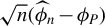 in
$\ell ^\infty (\mathbb {R}\times \Theta )$
 as
$n\to \infty $
 .
Lemma 2.1. If Assumptions 2.4 and 2.5 hold, then
$(\widehat {\phi }_n-\phi _P)\in \ell ^\infty (\mathbb {R}\times \Theta )$
 for all
$n\in \mathbb {Z}_+$
 . In addition,

as
$n\to \infty $
 , where
$\mathbb {G}_{0}$
 is some tight random element which almost surely takes values in
$\mathbb {D}_{\mathcal {L}0}$
 .
Define a function space

Define a map
$\mathcal {L}$
 on
$\mathbb {D}_{\mathcal {L}}$
 such that
$\mathcal {L}(\varphi )= \inf _{\theta \in \Theta } \int _{\mathbb {R}} \left[ \varphi (x,\theta ) \right]^2 \;\mathrm {d} \nu (x)$
 for every
$\varphi \in \mathbb {D}_{\mathcal {L}}$
 . Then under Assumptions 2.1–2.5, the null and the alternative hypotheses can be expressed as

To test the null hypothesis in (8), we set the test statistic to
$n \mathcal {L} ( \widehat {\phi }_n )$
 .
Next, we show that the map
$\mathcal {L}$
 is Hadamard directionally differentiable, but its Hadamard directional derivative is degenerate under
$\mathrm {H}_0$
 .Footnote
3
Define

The following lemma provides the Hadamard directional derivative of
$\mathcal {L}$
 and its first-order degeneracy under
$\mathrm {H}_0$
 .
Lemma 2.2. If Assumptions 2.3 and 2.4 hold, then
$\mathcal {L}$
 is Hadamard directionally differentiable at
$\phi _P\in \mathbb {D}_{\mathcal {L}}$
 tangentially to
$\mathbb {D}_{\mathcal {L}0}$
 with the Hadamard directional derivative

where
$\Theta _0(\phi _P)= {\mathrm{arg\,min}}_{\theta \in \Theta }\int _{\mathbb {R}} \left[ \phi _P (x,\theta ) \right]^2 \;\mathrm {d} \nu (x)$
 . Moreover, if
$\phi _P\in \mathbb {D}_0$
 , then the derivative
$\mathcal {L}^{\prime }_{\phi _P}$
 is well defined on the whole of
$\ell ^\infty (\mathbb {R}\times \Theta )$
 with
$\mathcal {L}^{\prime }_{\phi _P}(h)=0$
 for every
$h\in \ell ^\infty (\mathbb {R}\times \Theta )$
 .
The first-order degeneracy of
$\mathcal {L}$
 under
$\mathrm {H}_0$
 implies that we may need to find the second-order Hadamard directional derivative of
$\mathcal {L}$
 .Footnote
4
We assume the following conditions to guarantee the existence of the second-order Hadamard directional derivative of
$\mathcal {L}$
 .
Assumption 2.6. The function
$\phi _P$
 is twice differentiable with respect to
$\theta $
 , and the second partial derivative satisfies

where
$\left\Vert \cdot \right\Vert _{2}$
 denotes the
$\ell ^2$
 operator norm of a matrix.
Assumption 2.7. The set
$\Theta _0\equiv \{\theta \in \Theta :\int _{\mathbb {R}} \left[ \phi _P (x,\theta ) \right]^2 \;\mathrm {d} \nu (x)=0\}\subset \mathrm {int}(\Theta )$
 , and there exist
$\kappa \in (0,1]$
 ,
$\overline {\varepsilon }>0$
 , and
$C>0$
 such that for all
$\varepsilon \in (0,\overline {\varepsilon })$
 ,

We provide Assumptions 2.6 and 2.7 following the basic idea of Chen and Fang (Reference Chen and Fang2019b). Assumption 2.6 requires the boundedness of the second partial derivative of
$\phi _P$
 in the sense of (9). Assumption 2.7 requires that the set
$\Theta _0$
 is in the interior of
$\Theta $
 and it is well separated. The condition in (10) is similar to the partial identification assumption used in Chernozhukov et al. (Reference Chernozhukov, Hong and Tamer2007, p. 1265). It is worth noting that these conditions are sufficient but not necessary for our results, as also mentioned by Chen and Fang (Reference Chen and Fang2019b). We impose such high-level conditions for theoretical completeness. In Section 4, we verify these assumptions for a conditional moment restriction model.
Lemma 2.3. If Assumptions 2.3, 2.4, 2.6, and 2.7 hold, and
$\phi _P\in \mathbb {D}_0$
 , then the function
$\mathcal {L}$
 is second-order Hadamard directionally differentiable at
$\phi _P$
 tangentially to
$\mathbb {D}_{\mathcal {L}0}$
 with the second-order Hadamard directional derivative

where
$\Phi '(\theta ): \mathbb {R}\to \mathbb {R}^{d_{\theta }}$
 with

and
$\mathscr {H}:\Theta \to \ell ^\infty (\mathbb {R})$
 with
$\mathscr {H}(\theta )(x)=h(x,\theta )$
 for every
$(x,\theta )\in \mathbb {R}\times \Theta $
 .
Remark 2.1. Lemma 2.3 provides the explicit expression of the complicated second-order Hadamard directional derivative of
$\mathcal {L}$
 . We employ a numerical method that does not require exploring this function form.
With Lemma 2.3, the asymptotic null distribution of the test statistic
$n\mathcal {L}( \widehat {\phi }_n )$
 is obtained by applying the second-order delta method.


2.3 Bootstrap Procedure
The distribution of
$\mathcal {L}^{\prime \prime }_{\phi _P}\left( \mathbb {G}_0 \right)$
 in Proposition 2.2 is unknown because both the function
$\mathcal {L}^{\prime \prime }_{\phi _P}$
 and the stochastic process
$\mathbb {G}_0$
 depend on the unknown underlying distribution P. Motivated by Hong and Li (Reference Hong and Li2018) and Chen and Fang (Reference Chen and Fang2019b), we propose to approximate
$\mathcal {L}^{\prime \prime }_{\phi _P}$
 by a consistent estimator and approximate the distribution of
$\mathbb {G}_0$
 by bootstrap.Footnote
5
We use the numerical second-order Hadamard directional derivative
$\widehat {\mathcal {L}}^{\prime \prime }_n$
 to approximate
$\mathcal {L}^{\prime \prime }_{\phi _P}$
 , which is defined as

for all
$h\in \ell ^\infty (\mathbb {R}\times \Theta )$
 , where
$\left\{ \tau _n \right\}$
 is a sequence of tuning parameters satisfying the assumption below.Footnote
6
Assumption 2.8.
$\left\{ \tau _n \right\}\subset \mathbb {R}_+$
 is a sequence of scalars such that
$\tau _n\downarrow 0$
 and
$\tau _n \sqrt {n}\to \infty $
 as
$n\to \infty $
 .
Assumption 2.8 provides the rate at which
$\tau _n\downarrow 0$
 . Under this condition, we show that
$\widehat {\mathcal {L}}^{\prime \prime }_n$
 approximates
$\mathcal {L}^{\prime \prime }_{\phi _P}$
 well in the following lemma.
Lemma 2.4. If Assumptions 2.1–2.8 hold and
$\mathrm {H}_0$
 is true (
$\phi _P\in \mathbb {D}_0$
 ), then for every sequence
$\left\{ h_n \right\}\subset \ell ^\infty (\mathbb {R}\times \Theta )$
 and every
$h\in \mathbb {D}_{\mathcal {L}0}$
 such that
$h_n\to h$
 in
$\ell ^\infty (\mathbb {R}\times \Theta )$
 as
$n\to \infty $
 , we have

We next approximate the distribution of
$\mathbb {G}_0$
 via bootstrap. The bootstrap sample
$\mathbf {Z}_n^*=\{Z_i^*\}_{i=1}^n$
 is i.i.d. drawn from the empirical distribution
$\widehat {P}_n$
 of the original sample
$\mathbf {Z}_n$
 . Equivalently,
$\mathbf {Z}_n^*$
 is a random sample of size n, drawn from the set
$\mathbf {Z}_n$
 with replacement. Let
$\widehat {P}_n^*$
 be the empirical distribution of
$\mathbf {Z}_n^*$
 . Then the bootstrap version of
$\widehat {\phi }_n$
 is
$\widehat {\phi }_n^*$
 such that

for every
$(x,\theta )\in \mathbb {R}\times \Theta $
 .
Example 1.1 (Cont)
It follows by definition that

for every
$(x,\theta )\in \mathbb {R}\times \Theta $
 , where
$Z_i^*=(X_i^*,Y_i^*)$
 .
Example 1.2 (Cont)
Define

for every
$x\in \mathbb {R}$
 . Then

for every
$(x,\theta )\in \mathbb {R}\times \Theta $
 .
Example 1.3 (Cont)
Define

for every
$x\in \mathbb {R}$
 . Then

for every
$(x,\theta )\in \mathbb {R}\times \Theta $
 .
Example 1.4 (Cont)
Define
$\widehat {P}_n^*$
 as the empirical distribution of
$\{Z_i^*\}_{i=1}^n$
 with
$Z_i^*=(X_i^*,Y_i^*)$
 . Let
$\widehat {P}^*_{X,n}$
 and
$\widehat {P}^*_{Y,n}$
 be the marginal distributions of
$\widehat {P}_n^*$
 , that is, the (marginal) empirical distributions of
$\left\{ X_i^* \right\}_{i=1}^{n}$
 and
$\left\{ Y_i^* \right\}_{i=1}^{n}$
 , respectively. It follows that

for every
$(x,\theta )\in \mathbb {R}\times \Theta $
 . Define
$\widehat {F}_{n}^*$
 and
$\widehat {G}_{n}^*$
 to be the (marginal) empirical distribution functions of
$\left\{ X_i^* \right\}_{i=1}^{n}$
 and
$\left\{ Y_i^* \right\}_{i=1}^{n}$
 , respectively, such that for every
$x\in \mathbb {R}$
 ,

This implies that
$\widehat {\phi }_n^*(x,\theta )=\widehat {F}_{n}^* (x)-\widehat {G}_{n}^*\left( (x-\theta _1)/\theta _2 \right)$
 for every
$(x,\theta )\in \mathbb {R}\times \Theta $
 .
The following lemma establishes the conditional weak convergence of
$\sqrt {n}(\widehat {\phi }_n^*-\widehat {\phi }_n)$
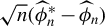 in probability as
$n\to \infty $
 .
Lemma 2.5. If Assumption 2.5 holds, then as
$n\to \infty $
 ,

and
$\sqrt {n}( \widehat {\phi }_n^*-\widehat {\phi }_n )$
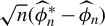 is asymptotically measurable, where
$\mathbb {G}_0$
 is defined as in Lemma 2.1.
With the numerical estimator
$\widehat {\mathcal {L}}^{\prime \prime }_n$
 for
$\mathcal {L}^{\prime \prime }_{\phi _P}$
 and a suitable bootstrap approximation
$\sqrt {n}( \widehat {\phi }_n^*-\widehat {\phi }_n )$
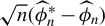 for
$\mathbb {G}_0$
 at hand, we can naturally approximate the distribution of
$\mathcal {L}^{\prime \prime }_{\phi _P}\left( \mathbb {G}_0 \right)$
 by the conditional distribution of the bootstrap test statistic
$\widehat {\mathcal {L}}^{\prime \prime }_n \{ \sqrt {n}( \widehat {\phi }_n^*-\widehat {\phi }_n ) \}$
 given the original sample. This is justified by the following proposition.
Proposition 2.3. If Assumptions 2.1–2.8 hold and
$\mathrm {H}_0$
 is true (
$\phi _P\in \mathbb {D}_0$
 ), then

as
$n\to \infty $
 .
2.4 Asymptotic Properties
Now we construct the test for the null hypothesis
$\mathrm {H}_0$
 . For a given level of significance
$\alpha \in (0,1)$
 , define the bootstrap critical value

In practice,
$\widehat {c}_{1-\alpha ,n}$
 may be approximated by the
$1-\alpha $
 empirical quantile of the
$n_B$
 independently generated bootstrap test statistics, with
$n_B$
 set to be as large as computationally feasible. We reject
$\mathrm {H}_0$
 if and only if
$n\mathcal {L} ( \widehat {\phi }_n )>\widehat {c}_{1-\alpha ,n}$
 . The following theorem shows that the proposed test is asymptotically size controlled and consistent.
Theorem 2.1. Suppose that Assumptions 2.1–2.8 hold.
-
(i) If $\mathrm {H}_0$
 is true and the CDF of
$\mathcal {L}^{\prime \prime }_{\phi _P}\left( \mathbb {G}_0 \right)$
is strictly increasing and continuous at its
$1-\alpha $
quantile, then $$ \begin{align*} \lim_{n\to\infty} \mathbb{P}\left( n \mathcal{L}( \widehat{\phi}_n )>\widehat{c}_{1-\alpha,n} \right) = \alpha. \end{align*} $$
-
(ii) If $\mathrm {H}_0$
is false, then $$ \begin{align*} \lim_{n\to\infty} \mathbb{P}\left( n \mathcal{L}( \widehat{\phi}_n )>\widehat{c}_{1-\alpha,n} \right)=1. \end{align*} $$


2.5 Local Power
In this section, we consider the local power of the test following the discussion in Chen and Fang (Reference Chen and Fang2019b). For each
$n\in \mathbb {Z}_+$
 , let the sample
$\mathbf {Z}_n=\{Z_i\}_{i=1}^n$
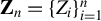 be distributed according to the joint law
$P_n^n=\prod _{i=1}^n P_n$
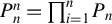 , where
$P_n$
 is a probability distribution on
$(\mathbb {R}^{d_z}, \mathscr {B}(\mathbb {R}^{d_z}))$
 with
$P_n(B)=\mathbb {P}(Z_i\in B)$
 for every Borel set B. That is, for each
$n\in \mathbb {Z}_+$
 , the observations
$Z_1,\ldots ,Z_n$
 are i.i.d. with distribution
$P_n$
 . We suppose that the null hypothesis
$\mathrm {H}_0$
 is false for each
$P_n$
 , that is, for all
$\theta \in \Theta $
 ,
$P_n(\psi _{x,\theta })\ne 0$
 for some
$x\in \mathbb {R}$
 . Suppose that
$P_n$
 converges (in a way as described in the following assumption) to the probability measure P, and that P satisfies
$\mathrm {H}_0$
 , that is, for some
$\theta \in \Theta $
 ,
$P(\psi _{x,\theta })= 0$
 for all
$x\in \mathbb {R}$
 .
Assumption 2.9. The probability distributions
$P_n$
 and P satisfy that

for some measurable function
$v_0:\mathbb {R}^{d_z}\to \mathbb {R}$
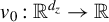 , where
$\mathrm {d}P_n^{1/2}$
 and
$\mathrm {d}P^{1/2}$
 denote the square roots of the densities of
$P_n$
 and P, respectively.
Our local power results rely on Assumption 2.9, which is similar to (3.10.10) of van der Vaart and Wellner (Reference van der Vaart and Wellner1996). The following proposition states formally the local power property of the test.
Proposition 2.4. Suppose that Assumptions 2.1–2.9 hold and
$\sup _{f\in \Psi } |P_n(f^2)| =O(1)$
 . Then
$\sqrt {n}( \widehat {\phi }_n-\phi _P )\leadsto \mathbb {G}_0+\zeta _P$
 , where
$\mathbb {G}_0$
 is some tight random element, and
$\zeta _P(x,\theta )= P(\psi _{x,\theta }v_0)$
 for every
$(x,\theta )\in \mathbb {R}\times \Theta $
 . Furthermore, if the CDF of
$\mathcal {L}^{\prime \prime }_{\phi _P}(\mathbb {G}_0)$
 is strictly increasing and continuous at its
$1-\alpha $
 quantile
$c_{1-\alpha }$
 , then it follows that

Proposition 2.4 follows from Lemma C.1 of Chen and Fang (Reference Chen and Fang2019b) and provides lower bounds for the power of the test under local perturbations to the null.
3 DEPENDENT DATA
This section considers cases where the observations
$\{Z_i\}_{i=1}^n$
 may be dependent. For results established in Section 2, it is worth noting that Lemmas 2.2–2.4, Propositions 2.1–2.3, and Theorem 2.1 do not directly rely on the i.i.d. nature of the data observations, possibly given the consistency and weak convergence of
$\widehat {\phi }_n$
 (Lemma 2.1) and the conditional weak convergence of
$\widehat {\phi }_n^*$
 in probability (Lemma 2.5). Thus, to obtain the asymptotic properties of the proposed test in dependent samples, it suffices to establish the consistency and weak convergence of
$\widehat {\phi }_n$
 and the conditional weak convergence of
$\widehat {\phi }_n^*$
 in probability under dependency.
A sequence of
$d_z$
 -dimensional random vectors,
$\{Z_i:i\in \mathbb {Z}\}$
 , is said to be strictly stationary, if for all
$\{i_1,\ldots ,i_n\}\subset \mathbb {Z}$
 and all
$n\in \mathbb {Z}_+$
 , the joint distribution of
$(Z_{i_1+k},\ldots ,Z_{i_n+k})$
 does not depend on k. For
$-\infty \le s\le t \le \infty $
 , let
$\mathscr {S}_{s}^{t}$
 be the
$\sigma $
 -field generated by
$\{Z_s,\ldots , Z_t\}$
 . Following Equation (II) of Volkonskii and Rozanov (Reference Volkonskii and Rozanov1959) and (1.1) of Arcones and Yu (Reference Arcones and Yu1994), the
$\beta $
 -mixing coefficient
$\beta _k$
 of the sequence
$\{Z_i:i\in \mathbb {Z}\}$
 is defined as

and
$\{Z_i:i\in \mathbb {Z}\}$
 is said to be
$\beta $
 -mixing if and only if
$\beta _k\to 0$
 as
$k\to \infty $
 .
Throughout our discussion of cases with dependent data, we assume that the sample
$\mathbf {Z}_n=\{Z_i:i=1,\ldots , n\}$
 is a finite segment of the strictly stationary sequence
$\{Z_i:i\in \mathbb {Z}\}$
 in which the common marginal distribution of
$Z_i$
 is P. We impose the following assumptions.
Assumption 3.1. The class
$\Psi =\{\psi _{x,\theta }:(x,\theta )\in \mathbb {R}\times \Theta \}$
 is a VC-subgraph class of functions satisfying (6) with
$P(\overline {\psi }^p)<\infty $
 for some
$p\in (2,\infty )$
 , where
$\overline {\psi }(z)=\sup _{f\in \Psi }|f(z)|$
 for every
$z\in \mathbb {R}^{d_z}$
 , and
$\Psi $
 is totally bounded under
$\Vert \cdot \Vert _{L^2(P)}$
 .Footnote
7
With p specified as in Assumption 3.1, we introduce the following condition for
$\beta _k$
 .
Assumption 3.2. The sequence
$\{Z_i:i\in \mathbb {Z}\}$
 is
$\beta $
 -mixing with coefficient
$\beta _k=O(k^{-q})$
 as
$k\to \infty $
 for some
$q>p/(p-2)$
 .
Assumption 3.1 emerges as one of the conditions in Theorem 2.1 of Arcones and Yu (Reference Arcones and Yu1994) and Theorem 1 of Radulović (Reference Radulović1996). Assumption 3.2 corresponds to one of the conditions in Theorem 1 of Radulović (Reference Radulović1996).
Let
$\widehat {\phi }_n$
 and
$\phi _P$
 be defined as in Section 2. The lemma below establishes the consistency and weak convergence of
$\widehat {\phi }_n$
 as
$n\to \infty $
 .
Lemma 3.1. If Assumptions 2.3, 2.4, 3.1, and 3.2 hold, then
$(\widehat {\phi }_n-\phi _P)\in \ell ^\infty (\mathbb {R}\times \Theta )$
 for all
$n\in \mathbb {Z}_+$
 . In addition,

as
$n\to \infty $
 , where
$\mathbb {G}_{0}$
 is tight and almost surely takes values in
$\mathbb {D}_{\mathcal {L}0}$
 .
To construct the bootstrap sample
$\mathbf {Z}_n^*=\{Z_i^*\}_{i=1}^n$
 , we follow Radulović (Reference Radulović1996) and use the moving blocks bootstrap (MBB) procedure. Recall that the original sample is
$\{Z_i\}_{i=1}^n$
 . Let
$b\in \mathbb {Z}_+$
 be the block size satisfying
$b\to \infty $
 and
$b/n\to 0$
 , and
$k\in \mathbb {Z}_+$
 be the number of blocks. Without loss of generality, we may assume that k and b satisfy
$kb=n$
 .Footnote
8
For
$i\in \{1,\ldots , b-1\}$
 , we set
$Z_{n+i}=Z_i$
 . Let the random variables
$I_1,\ldots , I_k$
 be i.i.d. from
$\mathrm {Unif}\{1,\ldots , n\}$
 and independent of the original sample. For all
$\ell \in \{1,\ldots ,k\}$
 and
$j\in \{1,\ldots ,b\}$
 , set the bootstrap observation
$Z_{(\ell -1)b+j}^*=Z_{I_\ell +j-1}$
 . That is, the bootstrap sample is

Let
$\widehat {P}_n^*$
 be the empirical distribution of
$\mathbf {Z}_n^*$
 . The bootstrap version of
$\widehat {\phi }_n$
 is defined as

for every
$(x,\theta )\in \mathbb {R}\times \Theta $
 .
We impose the assumption below on the block size b, which treats b as a function of n, that is,
$b=b(n)$
 . This assumption corresponds to one of the conditions in Theorem 1 of Radulović (Reference Radulović1996).
Assumption 3.3. The block size b is a function of the sample size n such that
$b=b(n)=O(n^r)$
 as
$n\to \infty $
 for some
$0<r<(p-2)/(2p-2)$
 .
The following lemma establishes the conditional weak convergence of
$\sqrt {n}(\widehat {\phi }_n^*-\widehat {\phi }_n)$
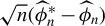 in probability.
Lemma 3.2. If Assumptions 3.1–3.3 hold, then as
$n\to \infty $
 ,

where
$\mathbb {G}_0$
 is defined as in Lemma 3.1.
Given the modification to the construction of the bootstrap sample, the remaining steps of the test follow the procedure in Section 2. For dependent data, the test is also asymptotically size controlled and consistent, as shown in Theorem 3.1.
Theorem 3.1. Suppose that Assumptions 2.1–2.4, 2.6–2.8, and 3.1–3.3 hold, and that
$\sqrt {n}(\widehat {\phi }_n^*-\widehat {\phi }_n)$
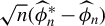 is asymptotically measurable.
-
(i) If $\mathrm {H}_0$
is true and the CDF of
$\mathcal {L}^{\prime \prime }_{\phi _P}\left( \mathbb {G}_0 \right)$
is strictly increasing and continuous at its
$1-\alpha $
quantile, then $$ \begin{align*} \lim_{n\to\infty} \mathbb{P}\left( n \mathcal{L}( \widehat{\phi}_n )>\widehat{c}_{1-\alpha,n} \right) = \alpha. \end{align*} $$
-
(ii) If $\mathrm {H}_0$
is false, then $$ \begin{align*} \lim_{n\to\infty} \mathbb{P}\left( n \mathcal{L}( \widehat{\phi}_n )>\widehat{c}_{1-\alpha,n} \right)=1. \end{align*} $$


4 MONTE CARLO EXPERIMENTS
In this section, we construct the Monte Carlo experiments based on the conditional moment restriction models with weak instrumental variables (IVs) in Jun and Pinkse (Reference Jun and Pinkse2009, Example II). Let
$y_i$
 be a scalar outcome variable,
$Y_i$
 be a scalar endogenous variable, and
$z_i$
 be a scalar IV. The model of interest is

for a true structural parameter
$\theta _0\in \Theta \subset \mathbb {R}$
 . We consider the null hypothesis

which is equivalent to

As noted by Jun and Pinkse (Reference Jun and Pinkse2009), there are several specification tests for (12) under strong point identification and the assumption that
$\theta _0$
 can be
$\sqrt {n}$
 -consistently estimated under the null (e.g., Bierens, Reference Bierens1990; Fan and Li, Reference Fan and Li1996, Reference Fan and Li2000; Zheng, Reference Zheng1996). Since
$\mathbb {E}_P[y_i-Y_i\theta _0|z_i]=0$
 almost surely for some
$\theta _0$
 under the null, typical estimators of
$\theta _0$
 include two-stage least squares (2SLS) and semi-parametric methods. However, when instruments are weak, these estimators of
$\theta _0$
 may be undesirable (e.g., Staiger and Stock, Reference Staiger and Stock1997; Stock and Wright, Reference Stock and Wright2000; Jun and Pinkse, Reference Jun and Pinkse2012), and thus two-step tests plugging in preliminary estimators of
$\theta _0$
 may not perform well.
Jun and Pinkse (Reference Jun and Pinkse2009) propose semi-parametric specification tests of conditional moment restrictions with weak instruments, which do not require a consistent first-step estimator. As shown in Theorems 1 and 2 of Jun and Pinkse (Reference Jun and Pinkse2009), their tests yield limiting rejection probabilities no greater than the nominal significance level under the null. Based on their Example II, Jun and Pinkse (Reference Jun and Pinkse2009) study the finite sample performance of their tests with weak instruments via Monte Carlo experiments. We first follow Jun and Pinkse (Reference Jun and Pinkse2009) and consider two cases under the null. In the first case (Case 1),
$\mathbb {E}_P[z_iY_i]=0$
 , that is, the rank condition fails and
$z_i$
 is not a valid instrument for
$Y_i$
 when estimating
$\theta _0$
 by 2SLS in two-step tests, which may be seen as an extreme case of weak instruments. Thus, the 2SLS estimator of
$\theta _0$
 that uses
$z_i$
 as the instrument for
$Y_i$
 is unreliable. In the second case (Case 2),
$\mathbb {E}_P[Y_i|z_i]\to 0$
 almost surely as
$n\to \infty $
 , that is, all measurable functions f of
$z_i$
 with
$\mathbb {E}_P[|f(z_i)Y_i|]<\infty $
 may be weak instruments for
$Y_i$
 when estimating
$\theta _0$
 by 2SLS in two-step tests because
$\mathbb {E}_P[f(z_i)Y_i]$
 may converge to
$0$
 . As discussed in Jun and Pinkse (Reference Jun and Pinkse2012), semi-parametric estimators of
$\theta _0$
 may also break down when
$\mathbb {E}_P[Y_i|z_i]$
 decays too fast in n. In addition, we consider a third case (Case 3), which is an extreme case of Case 2:
$\mathbb {E}_P[Y_i|z_i]= 0$
 almost surely.
As demonstrated in Tables 1 and 2 of Jun and Pinkse (Reference Jun and Pinkse2009), their tests improve greatly upon two-step plug-in methods in the presence of weak instruments, while they are often conservative, which is in line with their theoretical results. The proposed test in this article is asymptotically exactly size controlled and consistent under certain conditions, regardless of the strength of instruments. We numerically present these properties through Monte Carlo experiments, where the DGPs are designed for conditional moment restriction models with weak instruments as in the above cases.
Now we introduce the designs of our simulations. For i.i.d. samples, we follow the design of Jun and Pinkse (Reference Jun and Pinkse2009):

where
$\{(u_i,v_i,z_i):i=1,\ldots ,n\}$
 are i.i.d. with

The aforementioned three cases are realized in the following manner:
-
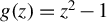
• Case 1: $\rho =0.5$
,
$\lambda =1$
, and
$g(z)=z^2-1$
. The moment
$\mathbb {E}_P[z_iY_i]=0$
. -
• Case 2: $\rho =-0.99$
,
$\lambda =0.07\sqrt {200/n}$
, and
$g(z)=z$
. The conditional moment
$\mathbb {E}_P[Y_i|z_i]\to 0$
almost surely as
$n\to \infty $
. -
• Case 3: $\rho =-0.5$
and
$\lambda =0$
. The conditional moment
$\mathbb {E}_P[Y_i|z_i]=0$
almost surely.










For each case, we consider four DGPs characterized by the values of
$\delta $
 :
-
• DGP (0): $\delta =0$
. The null is true. -
• DGP (1): $\delta =0.2$
. The null is false. -
• DGP (2): $\delta =0.6$
. The null is false. -
• DGP (3): $\delta =1$
. The null is false.


We also consider dependent data. For every DGP introduced above, we construct the dependent-data counterpart by generating
$\{z_i:i=1,\ldots ,n\}$
 as

where
$\{\varepsilon _{i}:i=1,\ldots ,n\}$
 are i.i.d.
$\mathcal {N}(0,1)$
 and independent of
$\{(u_i,v_i):i=1,\ldots ,n\}$
 .
Remark 4.1. For illustration of the high-level assumptions in Section 2.2, we consider Case 1 with
$\delta =0$
 . With
$\theta _{0}=1$
 ,
$\mathrm {H}_{0}$
 is true and thus

for all x. We have that for all
$\theta $
 ,

It follows that for all
$\theta $
 ,

The value
$\theta _{0}=1$
 satisfies
$\int _{\mathbb {R}}\phi _{P}\left( x,\theta _{0}\right) ^{2}\mathrm {d}\nu \left( x\right) =0$
 , so we have

For every
$\varepsilon>0$
 ,

This implies that

In this case, Assumptions 2.6 and 2.7 hold. The asymptotic limit of the test statistic is

Theorem 2.1(i) requires that the CDF of
$\mathcal {L}_{\phi _{P}}^{\prime \prime }\left( \mathbb {G}_{0}\right) $
 in (13) is strictly increasing and continuous at its
$1-\alpha $
 quantile.
The sample size is set to
$n\in \{100,200,400,800\}$
 . We set the tuning parameter
$\tau _n$
 as
$\tau _n=\sqrt {\ln (n)/n}$
 ,
$n^{-2/5}$
 ,
$n^{-1/3}$
 ,
$n^{-1/4}$
 ,
$n^{-1/5}$
 , and
$n^{-1/6}$
 , which all satisfy Assumption 2.8. For dependent data, the MBB involves an additional tuning parameter
$b(n)$
 . We set
$b(n)=n^{1/6}$
 ,
$n^{1/5}$
 ,
$n^{1/4}$
 , and
$n^{1/3}$
 . Recall that the test statistic involves an integration with respect to a measure
$\nu $
 and an infimum. The integration is approximated by an equally weighted average on the grid
$\{-3,-2.998, -2.996, \ldots , 3\}$
 of x, and the infimum is achieved by a search on the grid
$\{0.7, 0.702, 0.704, \ldots , 1.3\}$
 of
$\theta $
 . Furthermore, we apply the warp-speed method (Giacomini, Politis, and White, Reference Giacomini, Politis and White2013) to implement all the Monte Carlo experiments. Specifically, for each DGP and sample size, we generate
$1,000$
 samples and compute one original statistic
$n\mathcal {L}(\widehat {\phi }_n)$
 and one bootstrap statistic
$\widehat {\mathcal {L}}^{\prime \prime }_n[\sqrt {n}(\widehat {\phi }_n^*-\widehat {\phi }_n)]$
 for each sample. The critical value
$\widehat {c}_{1-\alpha ,n}$
 is approximated by the
$(1-\alpha )$
 -empirical quantile of the
$1,000$
 bootstrap statistics, and the rejection rate is computed by comparing the
$1,000$
 original statistics with the critical value
$\widehat {c}_{1-\alpha ,n}$
 .
We present some main simulation results in the following and leave the remaining results to Section E of the Supplementary Material. Tables 1–6 and Tables E.12–E.22 in the Supplementary Material show the rejection rates for different DGPs, tuning parameters, and nominal significance levels with measure
$\nu $
 being the probability measure of
$\mathcal {N}(0,10^2)$
 . Tables E.1–E.10 in the Supplementary Material display the rejection rates for Case 1 with the measure
$\nu $
 being the probability measure of
$\mathcal {N}(0,1)$
 or
$\mathcal {N}(0,5^2)$
 . The results are stable for different choices of
$\tau _n$
 ,
$b(n)$
 , and
$\nu $
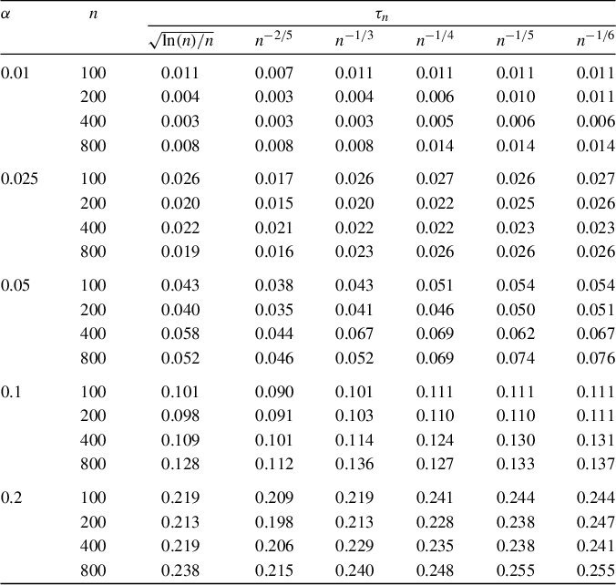
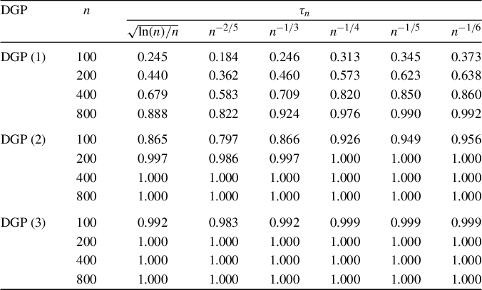
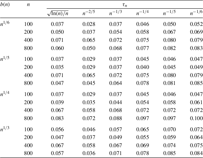
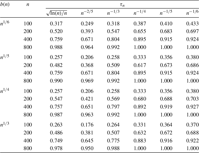
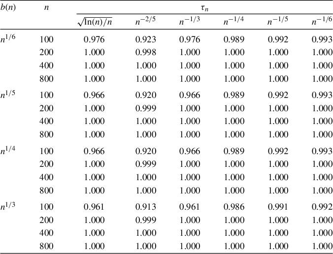
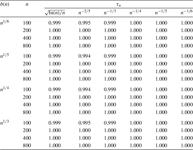
 . Most of the rejection rates under the null are close to the nominal significance levels. The rejection rates under the alternatives increase to one as the sample size n increases. For dependent samples, the rejection rates under the null may exceed the significance level
$\alpha $
 for some
$\tau _n$
 ,
$b(n)$
 , and
$\nu $
 as shown, for example, in Table 3. As we increase the sample sizes, the results become closer to
$\alpha $
 , as shown in Table E.11 in the Supplementary Material.
Size for Case 1 with i.i.d. data

Table 1 Long description
The table is organized into columns for alpha, n, and six different functional forms of tau sub n.
Header Row:
* Column 1: alpha
* Column 2: n
* Columns 3-8: tau sub n, with specific sub-headers: square root of {ln (n) all over n}, n super {-2/5}, n super {-1/3}, n super {-1/4}, n super {-1/5}, and n super {-1/6}.
Data Rows:
* For alpha = 0.01:
- n = 100: values range from 0.007 to 0.011.
- n = 200: values range from 0.003 to 0.011.
- n = 400: values range from 0.003 to 0.006.
- n = 800: values range from 0.008 to 0.014.
* For alpha = 0.025:
- n = 100: values range from 0.017 to 0.027.
- n = 200: values range from 0.015 to 0.026.
- n = 400: values range from 0.021 to 0.023.
- n = 800: values range from 0.016 to 0.026.
* For alpha = 0.05:
- n = 100: values range from 0.038 to 0.054.
- n = 200: values range from 0.035 to 0.051.
- n = 400: values range from 0.044 to 0.069.
- n = 800: values range from 0.046 to 0.076.
* For alpha = 0.1:
- n = 100: values range from 0.090 to 0.111.
- n = 200: values range from 0.091 to 0.111.
- n = 400: values range from 0.101 to 0.131.
- n = 800: values range from 0.112 to 0.137.
* For alpha = 0.2:
- n = 100: values range from 0.209 to 0.244.
- n = 200: values range from 0.198 to 0.247.
- n = 400: values range from 0.206 to 0.241.
- n = 800: values range from 0.215 to 0.255.
Power for Case 1 with i.i.d. data (
$\alpha =0.05$
 )

Table 2 Long description
The table is organized into columns for D G P, sample size n, and six different values of tau sub n. The tau sub n values are: square root of ln(n) all over n, n to the power of -2/5, n to the power of -1/3, n to the power of -1/4, n to the power of -1/5, and n to the power of -1/6.
* D G P (1):
- For n = 100, power values range from 0.184 to 0.373.
- For n = 200, power values range from 0.362 to 0.638.
- For n = 400, power values range from 0.583 to 0.860.
- For n = 800, power values range from 0.822 to 0.992.
* D G P (2):
- For n = 100, power values range from 0.797 to 0.956.
- For n = 200, power values range from 0.986 to 1.000.
- For n = 400 and 800, all power values are 1.000.
* D G P (3):
- For n = 100, power values range from 0.983 to 0.999.
- For n = 200, 400, and 800, all power values are 1.000.
Across all D G P models, power generally increases as the sample size n increases.
Size for Case 1 with dependent data (
$ \alpha =0.05$
 )

Table 3 Long description
The table is structured with three main headers: b(n), n, and tau sub n. The tau sub n header spans six sub-columns with different mathematical formulas: square root of {ln(n)/n}, n super -2/5, n super -1/3, n super -1/4, n super -1/5, and n super -1/6.
* For b(n) = n super 1/6:
- n = 100: values range from 0.028 to 0.052.
- n = 200: values range from 0.037 to 0.069.
- n = 400: values range from 0.065 to 0.080.
- n = 800: values range from 0.050 to 0.083.
* For b(n) = n super 1/5:
- n = 100: values range from 0.029 to 0.047.
- n = 200: values range from 0.029 to 0.049.
- n = 400: values range from 0.065 to 0.080.
- n = 800: values range from 0.045 to 0.085.
* For b(n) = n super 1/4:
- n = 100: values range from 0.029 to 0.047.
- n = 200: values range from 0.035 to 0.061.
- n = 400: values range from 0.058 to 0.072.
- n = 800: values range from 0.072 to 0.100.
* For b(n) = n super 1/3:
- n = 100: values range from 0.046 to 0.072.
- n = 200: values range from 0.037 to 0.064.
- n = 400: values range from 0.058 to 0.075.
- n = 800: values range from 0.036 to 0.085.
Power for DGP (1) of Case 1 with dependent data (
$ \alpha =0.05$
 )

Table 4 Long description
The table is structured with headers for b(n), n, and six variations of tau sub n.
* The tau sub n column headers are: square root of ln(n) all over n, n to the -2/5 power, n to the -1/3 power, n to the -1/4 power, n to the -1/5 power, and n to the -1/6 power.
* For b(n) = n to the 1/6 power:
- At n = 100, power values range from 0.249 to 0.433.
- At n = 200, power values range from 0.393 to 0.697.
- At n = 400, power values range from 0.671 to 0.924.
- At n = 800, power values range from 0.964 to 1.000.
* For b(n) = n to the 1/5 power:
- At n = 100, power values range from 0.206 to 0.380.
- At n = 200, power values range from 0.368 to 0.686.
- At n = 400, power values range from 0.671 to 0.924.
- At n = 800, power values range from 0.969 to 1.000.
* For b(n) = n to the 1/4 power:
- At n = 100, power values range from 0.206 to 0.380.
- At n = 200, power values range from 0.421 to 0.703.
- At n = 400, power values range from 0.651 to 0.927.
- At n = 800, power values range from 0.963 to 1.000.
* For b(n) = n to the 1/3 power:
- At n = 100, power values range from 0.176 to 0.370.
- At n = 200, power values range from 0.381 to 0.688.
- At n = 400, power values range from 0.645 to 0.922.
- At n = 800, power values range from 0.950 to 1.000.
Across all groups, power generally increases as n increases.
Power for DGP (2) of Case 1 with dependent data (
$ \alpha =0.05$
 )

Table 5 Long description
The table is organized with columns for b(n), n, and six variations of tau sub n. The tau sub n headers are: square root of ln(n) all over n, n super -2/5, n super -1/3, n super -1/4, n super -1/5, and n super -1/6.
* For b(n) = n super 1/6:
- n = 100: values range from 0.923 to 0.993.
- n = 200, 400, 800: all values are 1.000 except for n = 200 at n super -2/5 which is 0.998.
* For b(n) = n super 1/5:
- n = 100: values range from 0.920 to 0.993.
- n = 200: values are 1.000 except for n super -2/5 which is 0.999.
- n = 400, 800: all values are 1.000.
* For b(n) = n super 1/4:
- n = 100: values range from 0.920 to 0.993.
- n = 200: values are 1.000 except for n super -2/5 which is 0.999.
- n = 400, 800: all values are 1.000.
* For b(n) = n super 1/3:
- n = 100: values range from 0.913 to 0.992.
- n = 200: values are 1.000 except for n super -2/5 which is 0.999.
- n = 400, 800: all values are 1.000.
Power for DGP (3) of Case 1 with dependent data (
$ \alpha =0.05$
 )

Table 6 Long description
A data table showing power values across different parameters.
Header Row: The first column is b ( n ), the second is n, and the remaining six columns are grouped under tau sub n with the following specific values: square root of {ln ( n ) / n}, n super -2/5, n super -1/3, n super -1/4, n super -1/5, and n super -1/6.
Data Rows:
* For b ( n ) = n super 1/6: At n = 100, power values range from 0.995 to 1.000. For n = 200, 400, and 800, all power values are 1.000.
* For b ( n ) = n super 1/5: At n = 100, power values range from 0.994 to 1.000. For n = 200, 400, and 800, all power values are 1.000.
* For b ( n ) = n super 1/4: At n = 100, power values range from 0.994 to 1.000. For n = 200, 400, and 800, all power values are 1.000.
* For b ( n ) = n super 1/3: At n = 100, power values range from 0.995 to 1.000. For n = 200, 400, and 800, all power values are 1.000.
Across all tested values of b ( n ) and tau sub n, the power converges to 1.000 as the sample size n increases from 100 to 800.
4.1 Performance Improvement in Conditional Moment Restriction Models with Weak Instruments
Note that Cases 1 and 2 (
$n=200$
 ) with
$\delta =0$
 (under the null hypothesis) are identical to the DGPs in Tables 1 and 2 of Jun and Pinkse (Reference Jun and Pinkse2009), respectively. Thus, the results in Table 1 with
$n=100$
 and Table E.12 in the Supplementary Material with
$n=200$
 can be compared with those in Tables 1 and 2 of Jun and Pinkse (Reference Jun and Pinkse2009), respectively. We present the comparisons in Tables 7 and 8, where
$\widehat {T}_2(\widehat {\theta }_{*})$
 and
$\widehat {T}_{\mathrm {k}}(\widehat {\theta }_{*})$
 with
$\widehat {\theta }_{*}\in \{\widehat {\theta }_{\mathrm {2SLS}}, \widehat {\theta }_{\mathrm {SP}}\}$
 are two-step plug-in test statistics computed by using either a 2SLS or a semi-parametric estimator of
$\theta _0$
 as described in Jun and Pinkse (Reference Jun and Pinkse2009), and
$\widehat {T}_1(\widehat {\theta }_{\mathrm {CUE1}})$
 ,
$\widehat {T}_2(\widehat {\theta }_{\mathrm {CUE2}})$
 , and
$\widehat {T}_{\mathrm {k}}(\widehat {\theta }_{\mathrm {CUEk}})$
 are the test statistics proposed by Jun and Pinkse (Reference Jun and Pinkse2009).Footnote
9
Our test uses
$\tau _n=n^{-1/4}$
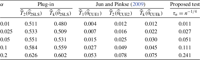
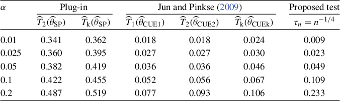
 for illustration. The plug-in method suffers from substantial size distortion. The tests of Jun and Pinkse (Reference Jun and Pinkse2009) improve upon the plug-in approach, but could be conservative as shown in their theoretical results. The proposed method achieves rejection rates closer to the nominal significance levels compared to the results of Jun and Pinkse (Reference Jun and Pinkse2009). These numerical observations provide supporting evidence for the theoretical results in the article.
Comparison with Table 1 of Jun and Pinkse (Reference Jun and Pinkse2009)

Table 7 Long description
The table consists of seven columns. The first column is alpha. The next two columns are under the heading Plug-in, containing T-hat sub 2 (theta-hat sub 2 S L S) and T-hat sub k (theta-hat sub 2 S L S). The following three columns are under the heading Jun and Pinkse 2009, containing T-hat sub 1 (theta-hat sub C U E 1), T-hat sub 2 (theta-hat sub C U E 2), and T-hat sub k (theta-hat sub C U E k). The final column is the Proposed test where tau sub n equals n to the power of minus 1/4.
Data rows by alpha value:
* Alpha 0.01: Plug-in (0.511, 0.480); Jun and Pinkse (0.004, 0.012, 0.012); Proposed test (0.011).
* Alpha 0.025: Plug-in (0.533, 0.509); Jun and Pinkse (0.007, 0.016, 0.022); Proposed test (0.027).
* Alpha 0.05: Plug-in (0.551, 0.531); Jun and Pinkse (0.015, 0.025, 0.030); Proposed test (0.051).
* Alpha 0.1: Plug-in (0.584, 0.559); Jun and Pinkse (0.027, 0.049, 0.045); Proposed test (0.111).
* Alpha 0.2: Plug-in (0.626, 0.602); Jun and Pinkse (0.053, 0.078, 0.075); Proposed test (0.241).
Comparison with Table 2 of Jun and Pinkse (Reference Jun and Pinkse2009)

Table 8 Long description
The table consists of seven columns. The first column is alpha. The next two columns are under the heading Plug-in, containing T-hat sub 2 (theta-hat sub S P) and T-hat sub k (theta-hat sub S P). The next three columns are under the heading Jun and Pinkse (2009), containing T-hat sub 1 (theta-hat sub C U E 1), T-hat sub 2 (theta-hat sub C U E 2), and T-hat sub k (theta-hat sub C U E k). The final column is the Proposed test with tau sub n = n to the power of minus 1/4.
Data rows by alpha value:
* Alpha 0.01: Plug-in (0.341, 0.362), Jun and Pinkse (0.018, 0.018, 0.024), Proposed (0.009).
* Alpha 0.025: Plug-in (0.360, 0.395), Jun and Pinkse (0.027, 0.027, 0.030), Proposed (0.023).
* Alpha 0.05: Plug-in (0.382, 0.419), Jun and Pinkse (0.036, 0.036, 0.046), Proposed (0.049).
* Alpha 0.1: Plug-in (0.422, 0.455), Jun and Pinkse (0.052, 0.056, 0.067), Proposed (0.109).
* Alpha 0.2: Plug-in (0.487, 0.519), Jun and Pinkse (0.077, 0.093, 0.106), Proposed (0.233).
5 CONCLUSION
This article provides a unified framework for inference on moment restriction models with nuisance parameters. We employ a new characterization that does not require the estimation of nuisance parameters, along with a numerical delta method to construct the test. The test is asymptotically size controlled and consistent. We conduct extensive Monte Carlo simulations to illustrate the finite sample properties of the proposed test. The numerical results show that the proposed method may achieve improvement in testing conditional moment restriction models with weak instruments. While the present article focuses primarily on models with finite-dimensional nuisance parameters, the proposed approach might be extended to moment restrictions involving infinite-dimensional nuisance parameters that have been widely investigated in the literature. This framework may also be applied to other inference problems in the presence of nuisance parameters.
SUPPLEMENTARY MATERIAL
Li, X., Song, X., & Sun, Z. (2026). Supplement to “Unified inference on moment restrictions with nuisance parameters,” Econometric Theory Supplementary Material. To view, please visit: https://doi.org/10.1017/S0266466626100528.
FUNDING STATEMENT
The work of X.S. was supported by the National Natural Science Foundation of China (Grant Nos. 72373007 and 72333001). The author also gratefully acknowledges the research support from the Center for Statistical Science of Peking University, China, and the Key Laboratory of Mathematical Economics and Quantitative Finance (Peking University) of the Ministry of Education, China. The work of Z.S. was supported by the National Natural Science Foundation of China (Grant No. 72103004).
COMPETING INTERESTS
The authors declare that no competing interests exist.









 Open access

