




No CrossRef data available.
ASYMPTOTIC ESTIMATION OF THE E-GINI INDEX
Published online by Cambridge University Press: 06 June 2003
Abstract
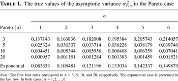
Under minimal assumptions on the distribution of income, we demonstrate that Chakravarty's empirical (1988, International Economic Review 29, 147–156) E-Gini index is consistent and asymptotically normal. We also derive an explicit formula for the asymptotic variance of the index and then construct a consistent and computationally straightforward estimator for it.Sincere thanks are due to the co-editor Oliver B. Linton and two anonymous referees whose constructive criticism, advice, and queries helped me in reshaping the paper considerably. As advised by a referee, I had the great pleasure of communicating with Garry F. Barrett and Stephen G. Donald and learning about their interesting and closely related results. The starting point of my work on the project was correspondence with Joseph L. Gastwirth in the spring of 2000 that resulted in our joint work on the S-Gini index. I am grateful to Joseph L. Gastwirth for his time, his advice, and his numerous suggestions that followed. The help, in addition to interest in the project, by Ying Zhang of the Statistical Laboratory at the University of Western Ontario is greatly appreciated; the analysis of the dependence of σF,α2 on parameters presented in Table 1 is due to her. This research was partially supported by an NSERC of Canada individual research grant at the University of Western Ontario.
Information
- Type
- Research Article
- Information
- Copyright
- © 2003 Cambridge University Press
1. INTRODUCTION
Measuring economic inequality, and, indeed, finding ways to properly measure it, is a challenging and important problem. A large number of indices of economic inequality, compatible with various axioms of fairness, have been proposed in the literature. For their definitions, related discussions, and further references, we refer, for example, to the books by Kakwani (1980a), Nygård and Sandström (1981), Sen (1997), Champernowne and Cowell (1998), Cowell (1998), Amiel and Cowell (1999), Silber (1999), and Atkinson and Bourguignon (2000).
In one way or another, many indices are based on the Lorenz curve, the notion of which was introduced by Lorenz (1905). Later, the notion was mathematically formalized by several authors, including Kendall and Stuart (1958), assuming that the (cumulative) distribution function F of “income” X ≥ 0 has a probability density function. Finally, assuming only that the mean μ := E(X) is finite and positive, Gastwirth (1971) gave the most general definition of the Lorenz curve as follows:

where

is the quantile function of F. Note that formula (1.2) defines the quantile function F−1 equally well for all distribution functions F. Thus, Gastwirth's definition (1.1) of LF is also valid for all distribution functions F, implying the outmost generality of it. For more information concerning quantiles and further references on the subject, we refer, for example, to Parzen (1979), Csörgő (1983, 1986), and Csörgő and Horváth (1993).
The value of the Lorenz curve LF does not depend on the measurement units of X. Furthermore, LF is always below the diagonal line I(t) := t. The diagonal I, on the other hand, has a special interpretation. Namely, if the income X is constant, meaning the absolute equality of incomes, then the corresponding Lorenz curve is identically I. This suggests that the income inequality in a society can be measured by the area between the diagonal I and the Lorenz curve LF corresponding to the society. Thus, the classical Gini index:

twice the area between I and LF. The Gini index GF has played a central role in measuring economic inequality since the works by Corrado Gini at the beginning of the 20th century. For historical and bibliographical notes on the subject we refer, for example, to David (1968) and Giorgi (1990, 1993).
The Gini index GF satisfies a number of axioms or, in other words, principles such as those of transfers, scale independence, and others; we refer to Dagum (1983) for an account of some of them. In particular, the Gini index satisfies (cf., e.g., Dagum, 1983) the Pigou–Dalton principle of transfers, which postulates that progressive (i.e., from rich to poor), rank order of incomes and also mean preserving transfers should decrease the values of inequality measures. Having verified the Pigou–Dalton principle, one “may go one step further and value more such a transfer between persons with given income difference if these incomes are lower than if they are higher” (Kolm, 1976b, p. 87). This describes the main idea of the principle of transfer sensitivity that has been discussed in great detail by Atkinson (1970), Mehran (1976), Kolm (1976a, 1976b), Kakwani (1980b), Shorrocks and Foster (1987), Chakravarty (1988), Sen (1997), Zheng (1997), Cowell (1998), Amiel and Cowell (1999), Silber (1999), and others.
Chakravarty (1988) notes that the Gini index GF fails to satisfy the so-called diminishing transfers axiom, whose meaning can be summarized as follows:
For two persons having incomes yi and yj with yi < yj, the reduction of inequality attributable to a rank preserving transfer from the person with income yi to another person with income yi − c (0 < c < yi) is greater than the reduction attributable to an equal rank preserving transfer from the person with income yj to someone with income yj − c. (Chakravarty, 1988, p. 147)
To rectify the situation, Chakravarty (1988) proposes a route that, in mathematical terms, can be described as follows. Let

denote the collection of the quantile functions F−1 corresponding to those distribution functions F whose mean is μ. Define the functional

on

by the formula

Note that the Gini index GF equals

. The functional
is linear, which appears (cf. Chakravarty, 1988, p. 148) to be the reason for the absence of the desired transfer sensitivity of the Gini index GF. Therefore, Chakravarty (1988) suggests modifying the functional

in such a way that the newly obtained functional would be strictly convex, that is, the quantity

would be strictly less than the sum of

, for any γ ∈ (0,1) and

. As an example of such a functional, Chakravarty (1988) suggests the following expression:

The functional

is strictly convex on

for any α > 1. Thus, we have Chakravarty's (1988) E(xtended)-Gini index

, the explicit formula of which is

We note in passing that in Zitikis (2002a) we argue that using (α + 1)1/α instead of 2 in definition (1.6) would be more natural from the mathematical point of view. Whether this modification is desirable from the econometric point of view still remains to be determined. We note here only that the asymptotic results presented in the following sections can easily be adapted to cover the proposed modification of GF,α.
We conclude this section with the note that Chakravarty (1988) suggests a functional even more general than

, which is

where φ : [0,1] → [0,∞) is a continuous, strictly increasing, and strictly convex function such that φ(0) = 0. As far as we are aware, the importance of functions φ other than φ(x) = xα has not yet been clarified in the econometric literature. In this paper we therefore restrict ourselves exclusively to the functional

, that is, to the E-Gini index GF,α defined in (1.6).
2. E-GINI ESTIMATOR
The distribution function F is generally unknown, and thus estimation theory for the E-Gini index GF,α is desirable. We shall now construct an empirical estimator for GF,α. Let X1,…,Xn be independent copies of X and let Fn be the empirical distribution function based on X1,…,Xn. Furthermore, let Fn−1 be the corresponding quantile function, which is defined by formula (1.2) with Fn instead of F. Replacing μ in definition (1.1) by the sample mean X of X1,…,Xn, and also replacing F−1 by its empirical counterpart Fn−1, we obtain the empirical Lorenz curve (Gastwirth, 1971):

Chakravarty's (1988) E-Gini extimator is now defined as follows:

The most recent and complete asymptotic theory for the E-Gini estimator Gn,α has been developed by Barrett and Donald (2000). In particular, Barrett and Donald (2000) prove that Gn,α is consistent and asymptotically normal under the following three assumptions.
(i) The support of F is in a bounded interval [yl,yu] for some 0 < yl < yu < ∞.
(ii) The distribution function F is twice differentiable.
(iii) The density function f = F′ is such that 0 < inf f (y) < sup f (y) < ∞, where both inf and sup are taken over all y ∈ [yl,yu] .
Naturally, it is of interest, and also of importance, to relax Assumptions (i)–(iii). There are several reasons for this. For example, minimal assumptions would assure the widest applicability of the obtained results and only minimal efforts would be required to verify such assumptions in practical situations. For a discussion of these issues, and further references on the subject, we refer to Beach and Davidson (1983).
The paper by Beach and Davidson (1983) was instrumental in developing the nonparametric statistical inference for Lorenz curves and associated indices of income inequality. For example, employing the results of Beach and Davidson (1983), Barrett and Pendakur (1995) investigate, among other things, the asymptotic behavior of the empirical E-Gini estimator. Both aforementioned papers, however, depend on a certain parameter K, which is the number of groups defined by percentiles into which the data under investigation are subdivided. Recently, employing the theory of empirical and quantile processes, Barrett and Donald (2000) have demonstrated that the introduction of the parameter K is unnecessary in the case of complete data. We also refer to the monograph by Csörgő, Csörgő, and Horváth (1986), and references therein, on related topics in the presence of complete data. When only grouped data are available, then the results by Gastwirth (1972), Gastwirth and Glauberman (1976), Aghevli and Mehran (1981), Beach and Davidson (1983), and Barrett and Pendakur (1995) become crucial in the development of the large sample based theory of statistical inference.
3. MAIN RESULTS
As we noted in the previous section, Gn,α is a natural estimator of GF,α. Obviously, the estimator is consistent under some assumptions on F. To show, however, that this is so under minimal assumptions requires some work, the result of which is the following theorem.
THEOREM 3.1. Let α ≥ 1. Then Gn,α is a strongly consistent estimator of GF,α.
Having thus proved the consistency of Gn,α, we would now like to use the estimator for constructing asymptotic confidence intervals for GF,α. For this reason, we need to obtain the sampling distribution of Gn,α. This we achieve in Theorem 3.2, which follows.
THEOREM 3.2. Let E(X2) < ∞ and α ≥ 1. Then the asymptotic distribution of

is normal with the mean 0 and the variance

where the quantity ΔF,α2 is defined by the formula

with σX2 denoting the variance of X and with

.
Several authors obtained slightly different, but equivalent, expressions for the variance σF,α2 in the classical Gini case (cf., e.g., Hoeffding, 1948, p. 314; Shorack and Wellner, 1986, p. 780). Obtaining explicit expressions for the variance σF,α2 has been a challenging problem in the general case. A review of various results along with the corresponding references can be found in Xu (2000). We shall now briefly discuss the source of the main difficulties. We start with a quote from Xu (2000): “the generalized-Gini-index estimators are functions of sample quantiles that are not regular statistics” (Xu, 2000, p. 223). Certainly, estimating quantiles is a challenging problem, the main difficulty arising due to the different tail behaviors of the theoretical and empirical quantile functions. However, it should be noted that when integrating the quantile functions F−1 and Fn−1, the differences between the resulting two integrals become less noticeable and, indeed, in the definitions of measures of income inequality the quantile functions play the roles of integrands. Thus, not separating integrals from quantile functions should be one of the main messages when working in the area. This approach in the case of the Lorenz curve LF was crucially utilized by Csörgő and Zitikis (1996), which resulted in the introduction of the general Vervaat process, and also by Csörgő, Gastwirth, and Zitikis (1998). Related developments in the case of the S-Gini index are presented in Zitikis and Gastwirth (2002).
As a result of the complex mathematical expression for σF,α2, determining the dependence of σF,α2 on the parameter α ≥ 1 is difficult when F is general. For this reason we now restrict ourselves to the Pareto and exponential distributions. We start with the Pareto distribution:

where x0 > 0 and λ > 0 are fixed parameters. To assure the existence of the second moment, we consider the values λ > 2 only. The values of σF,α2 for various λ and α are presented in Table 1. The asymptotic variance σF,α2 does not depend on x0.
The true values of the asymptotic variance σF,α2 in the Pareto case

Next we consider the exponential distribution

where γ > 0 is a fixed parameter. The corresponding values of σF,α2 are presented in the bottom row of Table 1. The asymptotic variance σF,α2 does not depend on γ.
4. ESTIMATION OF THE ASYMPTOTIC VARIANCE
Theorem 3.2 can be used for deriving confidence intervals for the E-Gini index GF,α. A standard argument based on Theorem 3.2 implies the following asymptotic 100(1 − p)% confidence interval:

where zp/2 is the p/2-percentile of the standard normal distribution and p ∈ (0,1) is any fixed number. The confidence interval of (4.1) is not yet readily applicable in practice because σF,α2 depends on the (unknown) distribution function F and, therefore, needs to be estimated. This can be achieved by replacing F everywhere in the definition of σF,α2 by the empirical distribution function Fn. The obtained estimator σFn,α2 is consistent, a statement that can be rigorously proved along the lines of the proof of Theorem 3.1. In Theorem 4.1, which follows, we use, however, a slight modification of this estimator so that practical implementation of it would be easier.
Let X and Sn2 denote, respectively, the sample mean and the sample variance of X1,…,Xn. Furthermore, let

for any i = 1,…,n − 1, and let

With these notations we are now in the position to formulate the following theorem.
THEOREM 4.1. Let E(X2) < ∞ and α ≥ 1. Then

is a strongly consistent estimator of σF,α2, where

We conclude this section with the note that when α = 1, which is the classical Gini case, then constructing estimators for σF,α2 is a central theme in a number of papers. For more details on this topic, we refer to Yitzhaki (1991) and references therein.
5. CONCLUDING REMARKS
As we already noted earlier, one of the main aims of this paper is to describe minimal assumptions under which the empirical E-Gini index is consistent and asymptotically normal. In view of this, we have restricted ourselves to the simplest but important case of independent and identically distributed random variables. It is of practical and theoretical interest to extend these results to dependent random variables and also to various other sampling schemes. Some work has been done in these two directions, though a large number of contributions are outside the area of the E-Gini index and, more generally, of measuring income inequality. We first mention contributions related to econometrics: Shao (1994), Zheng and Cushing (2001), Zheng (2001), and references therein. Contributions pertinent to both econometrics and stochastic processes are Yu (1993), Shao and Yu (1996), Csörgő and Yu (1996, 1999), Davydov and Zitikis (2001, 2002), and references therein. For related contributions in the context of stochastic processes, we refer to Davydov and Vershik (1998), Davydov and Thilly (1999), Thilly (1999), and references therein.
APPENDIX: PROOFS OF THEOREMS
We start with the note that the estimator Gn,α is a discretization of the following well-known and thoroughly investigated (cf., e.g., Barrett and Donald, 2000) E-Gini estimator:

Obviously, Gn,α* is GF,α with LF replaced by Ln. We shall find Gn,α* convenient in the proofs that follow.
We assume throughout the rest of the paper that the distribution function F is not degenerate. Otherwise, some technical details would arise, and one would have to deal with them in special ways, whereas the desired asymptotic results are always trivial in the degenerate case.
Proof of Theorem 3.1. We shall first prove that

We start with the formula

where p, x, and y are some positive real numbers to be specified subsequently. An application of formula (A.3) with

, and p = 1/α shows that statement (A.2) follows if

To prove (A.4) we use formula (A.3) with y = i/n − Ln(i/n), x = t − Ln(t), and p = α. In this way we obtain that, for any t ∈ [(i − 1)/n,i/n] ,

From bound (A.5) we see that statement (A.4) follows if the supremum on the right-hand side of bound (A.5) converges to 0 almost surely. To prove this, we use the following bound:

The first summand on the right-hand side of (A.6) is known in the literature as the Dobrushin distance between Fn and F (cf. Dobrushin, 1970). Thus,

(cf., e.g., Shorack and Wellner, 1986, exercise 9, p. 66). To prove that the second summand on the right-hand side of (A.6) converges to 0, we first note that, as a result of E(X) < ∞, the function

is continuous and thus is uniformly continuous on [0,1]. This implies the convergence of the second summand on the right-hand side of (A.6) to 0. The proof of statement (A.2) is complete.
In view of (A.2), Theorem 3.1 follows if

Choosing

, and p = 1/α in formula (A.3), we obtain that statement (A.8) is a consequence of the following statement:

Applying equality (A.3) once more but this time with y = t − Ln(t), x = t − LF(t), and p = α, we obtain (A.9) provided that

To prove (A.10), we proceed with the bound

The first summand on the right-hand side of (A.11) converges to 0 almost surely as a result of (A.7). The second summand converges to 0 because X is a strongly consistent estimator of μ, and the integral

does not exceed E(X) < ∞. The proof of statement (A.10) is now complete and thus that of (A.8) also. This proves Theorem 3.1. █
Proof of Theorem 3.2. We shall first prove that

The proof of (A.12) closely resembles that of statement (A.2). Therefore, we omit most of the details and only discuss the proof of the statement

We start the proof of (A.13) with the bound

Next, we estimate the integral on the right-hand side of (A.14) as follows:

Because E(X2) < ∞, the function

is continuous and, therefore, uniformly continuous on the interval [0,1]. This implies that the second summand on the right-hand side of (A.15) converges to 0. The first summand

is known in the literature as the Wasserstein distance between Fn and F. It is also known (cf., e.g., Shorack and Wellner, 1986, Corollary 1, p. 63) that d2(Fn,F) →a.s. 0 under the assumption E(X2) < ∞. This proves (A.13) and thus (A.12) also.
In view of (A.12), Theorem 3.2 follows if

where

denotes a mean zero normal random variable with the variance σF,α2. We proceed with the proof of (A.17) by rewriting formula (A.3) in the following form:

Using (A.18) with

, and p = 1/α, we obtain statement (A.17) if

. The latter can explicitly be written as follows:

To prove (A.19), we first apply formula (A.18) with y = t − Ln(t), x = t − LF(t), and p = α. We obtain the representation

The remainder term Qn,α(t) on the right-hand side of (A.20) is defined by the formula

Note that Qn,α(t) is asymptotically smaller than the main (i.e., the first) term on the right-hand side of (A.20). Therefore, using (A.20) we obtain (A.19) if

To prove (A.21), we start with the equality

where

Obviously,

Using statement (A.7) and the fact that

is asymptotically bounded in probability, we obtain from (A.23) that

converges to 0 in probability. Therefore, (A.22) implies statement (A.21) provided that

To prove statement (A.24), we use the representation

where Vn is the general Vervaat process (cf. Csörgő and Zitikis, 1996) defined by the formula

It is well known (cf., e.g., Zitikis, 1998) that the Vervaat process Vn is nonnegative and does not exceed −{Fn(F−1(t)) − t}{Fn−1(t) − F−1(t)}. Note that if t is a continuity point of F, then the latter statement can be written as the following inequality:

This implies the bound

Note that the use of (A.26) for proving (A.27) was legitimate because of the fact that the set of all discontinuity points of F has the Lebesgue measure 0. Thus, the value of the integral is not affected by removing the points. Now, by the classical Kolmogorov–Smirnov theorem,

is asymptotically bounded in probability. Furthermore, statement (A.7) implies that the integral on the right-hand side of (A.27) converges to 0 in probability. These facts taken together with (A.25) imply statement (A.24) provided that

The proof of (A.28) is straightforward. Note first that (cf., e.g., Shorack, 2000, formula (6), p. 116)

Thus, the integral on the left-hand side of (A.28) is the sum

of independent and identically distributed random variables Y1,Y2,…,Yn defined by the formula

By the classical central limit theorem, statement (A.28) holds if ΔF,α2 is the variance σY12 of Y1. Straightforward calculations show that this is the case. The proof of (A.21) is complete. █
Proof of Theorem 4.1. The proof of Theorem 4.1 follows the lines of the proof of Theorem 3.1. Naturally, the therein used assumption E(X) < ∞ should now be replaced by the stronger one E(X2) < ∞. We omit the technical details, noting only that analogous calculations in the case of the asymptotic variance of the S-Gini index are carried out by Zitikis (2002b). █
References
REFERENCES
Aghevli, B.B. &
F. Mehran
(1981)
Optimal grouping of income distribution data.
Journal of the American Statistical Association
76,
22–26.CrossRefGoogle Scholar
Amiel, Y. &
F.A. Cowell
(1999)
Thinking about Inequality.
Cambridge:
Cambridge University Press.
Atkinson, A.B.
(1970)
On the measurement of inequality.
Journal of Economic Theory
2,
244–263.CrossRefGoogle Scholar
Atkinson, A.B. &
F. Bourguignon (eds.)
(2000)
Handbook of Income Distribution.
Amsterdam:
Elsevier Science.
Barrett, G.F. &
S.G. Donald
(2000)
Statistical Inference with Generalized Gini Indices of Inequality and
Poverty.
Discussion paper 2002/01,
School of Economics, University of New South Wales.
Barrett, G.F. &
K. Pendakur
(1995)
The asymptotic distribution of the generalized Gini indices of
inequality.
Canadian Journal of Economics
28,
1042–1055.CrossRefGoogle Scholar
Beach, C.M. &
R. Davidson
(1983)
Distribution-free statistical inference with Lorenz curves and
income shares.
Review of Economic Studies
50,
723–735.CrossRefGoogle Scholar
Chakravarty, S.R.
(1988)
Extended Gini indices of inequality.
International Economic Review
29,
147–156.CrossRefGoogle Scholar
Champernowne, D.G. &
F.A. Cowell
(1998)
Economic Inequality and Income Distribution.
Cambridge:
Cambridge University Press.
Cowell, F.A.
(1998)
Measuring Inequality.
2nd ed.
London:
Prentice-Hall/Harvester.
Csörgő, M.
(1983)
Quantile Processes with Statistical Applications.
Philadelphia:
SIAM.
Csörgő, M.
(1986)
Quantile processes. In
S. Kotz,
N.L. Johnson, &
C.B. Read (eds.),
Encyclopedia of Statistical Sciences,
vol. 7, pp.
412–424.
New York:
Wiley.
Csörgő, M.,
S. Csörgő, &
L. Horváth
(1986)
An Asymptotic Theory for Empirical Reliability and Concentration
Processes.
Berlin:
Springer-Verlag.
Csörgő, M.,
J.L. Gastwirth, &
R. Zitikis
(1998)
Asymptotic confidence bands for the Lorenz and Bonferroni curves
based on the empirical Lorenz curve.
Journal of Statistical Planning and Inference
74,
65–91.CrossRefGoogle Scholar
Csörgő, M. &
L. Horváth
(1993)
Weighted Approximations in Probability and Statistics.
Chichester:
Wiley.
Csörgő, M. &
H. Yu
(1996)
Weak approximations for quantile processes of stationary sequences.
Canadian Journal of Statististics
24,
403–430.CrossRefGoogle Scholar
Csörgő, M. &
H. Yu
(1999)
Weak approximations for empirical Lorenz curves and their Goldie
inverses of stationary observations.
Advances in Applied Probability
31,
698–719.CrossRefGoogle Scholar
Csörgő, M. &
R. Zitikis
(1996)
Strassen's LIL for the Lorenz curve.
Journal of Multivariate Analysis
59,
1–12.CrossRefGoogle Scholar
Dagum, C.
(1983)
Income inequality measures. In
S. Kotz,
N.L. Johnson, &
C.B. Campbell (eds.),
Encyclopedia of Statistical Sciences,
vol. 4, pp.
34–40.
New York:
Wiley.
David, H.A.
(1968)
Gini's mean difference rediscovered.
Biometrika
55,
573–575.CrossRefGoogle Scholar
Davydov, Y. &
E. Thilly
(1999)
Réarrangements convexes de processus stochastiques.
Comptes Rendus de l'Académie des Sciences: Série
Mathématique
329,
1087–1090.CrossRefGoogle Scholar
Davydov, Y. &
A.M. Vershik
(1998)
Réarrangements convexes des marches aléatoires.
Annales de l'Institut Henri Poincaré:
Probabilités et Statistiques
34,
73–95.CrossRefGoogle Scholar
Davydov, Y. &
R. Zitikis
(2001)
Generalized Lorenz Curves and Convexifications of Stochastic
Processes.
Technical Report 359,
Laboratory for Research in Statistics and Probability, Carleton
University and University of Ottawa,
Ottawa.
Davydov, Y. &
R. Zitikis
(2002)
Convergence of generalized Lorenz curves based on stationary
ergodic random sequences with deterministic noise.
Statistics and Probability Letters
59,
329–340.CrossRefGoogle Scholar
Dobrushin, R.L.
(1970)
Describing a system of random variables by conditional
distributions.
Theory of Probability and Its Applications
15,
458–486.CrossRefGoogle Scholar
Gastwirth, J.L.
(1971)
A general definition of the Lorenz curve.
Econometrica
39,
1037–1039.CrossRefGoogle Scholar
Gastwirth, J.L.
(1972)
The estimation of the Lorenz curve and Gini index.
Review of Economics and Statistics
54,
306–316.CrossRefGoogle Scholar
Gastwirth, J.L. &
M. Glauberman
(1976)
The interpolation of the Lorenz curve and Gini index from grouped
data.
Econometrica
44,
479–483.CrossRefGoogle Scholar
Giorgi, G.-M.
(1990)
Bibliographic portrait of the Gini concentration ratio.
Metron
48,
183–221.Google Scholar
Giorgi, G.-M.
(1993)
A fresh look at the topical interest of the Gini concentration
ratio.
Metron
51,
83–98.Google Scholar
Hoeffding, W.
(1948)
A class of statistics with asymptotically normal distribution.
Annals of Mathematical Statistics
19,
293–325.CrossRefGoogle Scholar
Kakwani, N.C.
(1980a)
Income Inequality and Poverty: Methods of Estimation and Policy
Applications.
New York:
Oxford University Press.
Kendall, M.G. &
A. Stuart
(1958)
The Advanced Theory of Statistics, vol. 1:
Distribution theory.
New York:
Hafner Publishing.
Kolm, S.C.
(1976a)
Unequal inequalities, part I.
Journal of Economic Theory
12,
416–442.Google Scholar
Kolm, S.C.
(1976b)
Unequal inequalities, part II.
Journal of Economic Theory
13,
82–111.Google Scholar
Lorenz, M.C.
(1905)
Methods of measuring the concentration of wealth.
Journal of the American Statistical Association
9,
209–219.Google Scholar
Nygård, F. &
A. Sandström
(1981)
Measuring Income Inequality.
Stockholm:
Almqvist & Wiksell.
Parzen, E.
(1979)
Nonparametric statistical data modeling. With comments by John W.
Tukey, Roy E. Welsch, William F. Eddy, D.V. Lindley, Michael E. Tarter,
and Edwin L. Crow, and a rejoinder by the author.
Journal of the American Statistical Association
74,
105–131.Google Scholar
Sen, A.
(1997)
On Economic Inequality.
(Expanded edition with a substantial annexe by J.E. Foster & A.
Sen.)
Oxford:
Clarendon Press.
Shao, J.
(1994)
L-statistics in complex survey problems.
Annals of Statistics
22,
946–967.Google Scholar
Shao, Q.-M. &
H. Yu
(1996)
Weak convergence for weighted empirical processes of dependent
sequences.
Annals of Probability
24,
2098–2127.Google Scholar
Shorack, G.R.
(2000)
Probability for Statisticians.
New York:
Springer-Verlag.
Shorack, G.R. &
J.A. Wellner
(1986)
Empirical Processes with Applications to Statistics.
New York:
Wiley.
Shorrocks, A.F. &
J.E. Foster
(1987)
Transfer sensitive inequality measures.
Review of Economic Studies
54,
485–497.Google Scholar
Silber, J. (ed.)
(1999)
Handbook on Income Inequality Measurement.
Boston:
Kluwer Academic Publishers.
Thilly, E.
(1999)
Réarrangements Convexes des Trajectoires de Processus
Stochastiques.
Ph.D. Thesis,
University of Science and Technology of Lille,
Lille.
Xu, K.
(2000)
Inference for generalized Gini indices using the iterated-bootstrap
method.
Journal of Business and Economic Statistics
18,
223–227.Google Scholar
Yitzhaki, S.
(1991)
Calculating jackknife variance estimators for parameters of the
Gini method.
Journal of Business and Economic Statistics
9,
235–239.Google Scholar
Yu, H.
(1993)
A Glivenko-Cantelli lemma and weak convergence for empirical
processes of associated sequences.
Probabability Theory and Related Fields
95,
357–370.Google Scholar
Zheng, B. &
B.J. Cushing
(2001)
Statistical inference for testing inequality indices with dependent
samples.
Journal of Econometrics
101,
315–335.Google Scholar
Zheng, B.
(2001)
Statistical inference for poverty measures with relative poverty
lines.
Journal of Econometrics
10,
337–356.Google Scholar
Zitikis, R.
(1998)
The Vervaat process. In
B. Szyszkowicz (ed.),
Asymptotic Methods in Probability and Statistics: A Volume in
Honour of Miklós Csörgő, pp.
667–694.
Amsterdam:
Elsevier.
Zitikis, R.
(2002a)
Analysis of indices of economic inequality from a mathematical
point of view. (Invited Plenary Lecture at the 11th Indonesian
Mathematics Conference, State University of Malang, Indonesia.)
Matematika
8,
772–782.Google Scholar
Zitikis, R.
(2002b)
Large sample estimation of a family of economic inequality indices.
Pakistan Journal of Statistics
(Special Issue in Honour of Dr. S. Ejaz Ahmed)
18,
225–248.Google Scholar
Zitikis, R. &
J.L. Gastwirth
(2002)
Asymptotic distribution of the S-Gini index.
Australian and New Zealand Journal of Statistics
44,
439–446.Google Scholar
The true values of the asymptotic variance σF,α2 in the Pareto case
 You have
Access
- 13
- Cited by