

Days open (DO), the interval from calving to successful conception, is a crucial performance indicator in dairy farming. Extended DO can reduce the milk yield per cow per year by increasing the calving interval (Louca and Legates, Reference Louca and Legates1968; Olds et al., Reference Olds, Cooper and Thrift1979; Plaizier et al., Reference Plaizier, King, Dekkers and Lissemore1997). It can also shorten the productive lifespan of cows, leading to economic losses and increased replacement costs (Pinedo and De Vries, Reference Pinedo and De Vries2010). Additionally, extended DO is associated with various diseases (Bahonar et al., Reference Bahonar, Azizzadeh, Stevenson, Vojgani and Mahmoud2009), raising animal welfare concerns (Kolacz et al., Reference Kolacz, Jaśkowski and Ciorga2020).
Research has extensively studied factors affecting the DO in dairy cattle, including milk yield, health factors and management practices (Eicker et al., Reference Eicker, Gröhn and Hertl1996; Farin et al., Reference Farin, Slenning, Correa and Britt1994; Harman et al., Reference Harman, Casella and Gröhn1996). Additionally, health-related factors and common herd diseases have been shown to significantly impact DO (Lee et al., Reference Lee, Ferguson and Galligan1989; Maizon et al., Reference Maizon, Oltenacu, Gröhn, Strawderman and Emanuelson2004). Several region-specific studies have also validated these findings, underscoring the role of health factors, management practices and herd milk yield level in influencing DO (Bahonar et al., Reference Bahonar, Azizzadeh, Stevenson, Vojgani and Mahmoud2009; Temesgen et al., Reference Temesgen, Assen, Gizaw, Minalu and Mersha2022).
While prior research has shed light on factors influencing DO in dairy cattle, AI and machine learning can complement statistical approaches by modelling nonlinearities and temporal patterns that may be difficult to capture with conventional methods, thereby supporting, rather than replacing, established tools.
Predicting DO in advance enables proactive management (e.g., nutritional adjustments, targeted veterinary care, scheduling), and can illuminate how disease burden in one cycle may affect subsequent fertility. Such foresight supports selective culling and resource allocation decisions, potentially improving productivity and reducing costs.
Previous research has predominantly relied on survival analysis, a statistical technique designed for time-to-event studies. Specifically, these studies have leveraged the Cox proportional hazards model to examine the impact of covariates on the duration of the open period. While this conventional approach has proven effective in determining the influence of various factors on the open period, it is accompanied by several challenges that render it less suitable for predictive tasks.
One significant limitation of survival analysis is that many parametric and semi-parametric approaches in this field come with specific assumptions about the behaviour of hazard functions. For example, in the exponential model, it is assumed that the hazard (risk) is constant over time, implying a uniform rate of occurrence of the event of interest. Similarly, in the Cox proportional hazards model, the assumption is that the hazard ratios (HR), which describe the relative risks, are constant over time (Cox, Reference Cox1972). These assumptions may not hold in complex real-world scenarios, such as the effect of diseases on reproductive performance over time.
Another limitation of these models is their inability to harness the power of historical data from past lactation cycles and previous DO values. In dairy farming, the reproductive history of individual animals plays a crucial role in their future fertility and DO duration. Survival analysis, rooted in the examination of time-to-event data, can under-represent longitudinal reproductive history across cycles.
Recurrent neural networks (RNNs) are well-suited to sequence data and can leverage information from prior lactations (Hochreiter and Schmidhuber, Reference Hochreiter and Schmidhuber1997), making fewer parametric assumptions than many survival models but often requiring more data, careful tuning and safeguards against overfitting and information leakage. These strengths and limitations make them particularly relevant for predicting ‘days open’, a trait shaped by nonlinear interactions and temporal dependencies that are difficult to capture with parametric hazards alone. To ensure robust evaluation, this study applies leakage-averse data splits, preprocessing and imputation, regularisation and early stopping and systematic hyperparameter tuning, with performance benchmarked against conventional baselines (Cox, multi-layer perceptron [MLP]) and reported as mean performance across multiple runs to stabilise estimates.
Consistent with this rationale, RNN models have been increasingly utilised in various tasks, including the prediction and analysis of dairy cattle behaviour and health. For instance, they have been used to predict calving events (Keceli et al., Reference Keceli, Catal, Kaya and Tekinerdogan2020; Liseune et al., Reference Liseune, Salamone, Van den Poel, van Ranst and Hostens2021), daily milk yield (Zhang et al., Reference Zhang, Yang, Yu, Cheng and Liu2020), recognition of cow’s behaviour patterns (Peng et al., Reference Peng, Kondo, Fujiura, Suzuki, Wulandari and Itoyama2019; Yin et al., Reference Yin, Wu, Shang, Jiang and Song2020), lameness detection (Wu et al., Reference Wu, Wu, Yin, Jiang, Wang, He and Song2020) and support for selective antibiotic treatment strategies during the dry period (Rafael, Reference Rafael2023). In the realm of cattle reproduction, they have also been used for predicting pregnancy loss from activity data (Lin et al., Reference Lin, Kenéz, McArt and Li2023), oestrus detection (Ma et al., Reference Ma, Pan, Chen and Liu2020; Wang et al., Reference Wang, Bai, Gao, Li, Zhao, Li and Zhang2022) and pregnancy detection (Singla et al., Reference Singla, Jain, Tiwari, Kukreja and Sharma2023). These studies collectively demonstrate the versatility and effectiveness of RNNs in leveraging sequential information for various predictive tasks in dairy farming. More broadly, the utility of artificial neural networks for modelling complex systems is well established (Ekonomou et al., Reference Ekonomou, Fotis, Maris and Liatsis2007; Fotis et al., Reference Fotis, Ekonomou, Maris and Liatsis2007).
However, the potential of RNNs for forecasting DO in dairy cows has not yet been fully explored. Prior studies have largely relied on survival analysis, which imposes restrictive assumptions and does not fully exploit longitudinal reproductive histories across cycles. This work addresses that gap by formulating DO prediction as a sequence modelling task over repeated lactations and benchmarking recurrent architectures (long short-term memory [LSTM] and bidirectional LSTM [BiLSTM]) against both a feed-forward neural network (MLP) and a Cox proportional hazards model. Predictors are restricted to information available at the relevant decision point, and performance is evaluated using concordance index, mean absolute error (MAE), mean squared error (MSE) and R2, with results reported as averages across 10 independent runs to ensure stability. The overarching objective is to determine whether sequence-based models can provide more accurate and practical forecasts of DO, thereby supporting herd management, profitability and animal welfare.
The main contributions of this study are as follows:
1. Construction of a dataset comprising 16,472 breeding records, aligned to ensure the temporal validity of predictors.
2. Formulation of DO forecasting as a sequence modelling problem across consecutive lactation cycles.
3. Systematic comparison of MLP, LSTM, BiLSTM and Cox models, repeated across 10 runs, using multiple evaluation metrics (MAE, MSE, R2 and concordance index).
4. Empirical demonstration that LSTM-based models substantially reduce prediction error and improve concordance relative to conventional baselines.
Materials and methods
Study area
This study utilised data from the Helal Agro-Industry Co., a commercial dairy farm associated with the Iranian Red Crescent Investment Company. The farm is located near Neyshabur, the second-largest city in the Razavi Khorasan Province in the Northeast of Iran, nestled in a fertile plain at the foot of the Binalud Mountain Range, and is characterised by a cold, semi-arid climate.
The commercial dairy herds in this region primarily consist of Holstein-Friesian cattle. On this farm, these cows calve year-round, are rebred through artificial insemination and are housed in open-shed barns. They are milked three times a day, with their diet focusing on total mixed rations of corn silage, alfalfa hay and concentrates.
In terms of record-keeping and efficient data management, the agricultural enterprise utilises the Modiran Farmer software, a widely adopted solution within Iranian dairy farming circles owing to its proficiency in data documentation and streamlined report generation. This software leverages the Microsoft Structured Query Language (SQL) Server database infrastructure to facilitate the storage of pertinent information. The dataset encompasses a diverse array of tables containing entries spanning various aspects such as reproduction, milking, health profiles, genetic insights and broader characteristic attributes. The database spans from January 1994 to May 2023, encapsulating a substantial historical period.
Data extraction
An SQL query was executed against the database to generate a dataset of breeding records and their corresponding features. Cows that had at least two valid subsequent calving events recorded in the database were eligible for inclusion in the extracted dataset, and in total, 16,472 records from 5,557 cows that met these criteria were used for model development. For each breeding record, 22 features were retrieved, encompassing covariates related to milking, reproduction, management factors and health. To ensure strict temporal validity, all predictors were aligned to be observed at or before the relevant decision point for the target reproductive cycle. A summary of pre-imputation descriptive statistics and completeness is reported in Table 1.
Extracted features for each breeding cycle

The query’s conditions were defined to ascertain the utmost relevance and integrity of the data gathered. Only those body and motion scores falling within predefined acceptable ranges were incorporated into the records: 1 to 9 for body scores, which signify the cows’ physical well-being and 1 to 5 for motion scores, indicating the cows’ mobility. The scores were assessed monthly for each cow. A noticeable rate of missing values was observed, often due to the cow’s absence during measurement sessions. To bolster accuracy, each cow’s monthly body and motion scores were averaged over the interval between two consecutive calving events. This approach helped mitigate potential discrepancies stemming from missing or incomplete data.
The database was queried to determine the occurrence of specific health disorders during the inter-calving period or at calving (stillbirth, dystocia, retained foetal membranes, lameness, mastitis, ketosis, retained placenta, displaced abomasum); records containing relevant disease codes or keywords were flagged accordingly. Management-related metrics were also calculated, including age at calving (days), number of times bred before successful conception and calving season encoded as four binary variables representing winter (December–February), spring (March–May), summer (June–August) and fall (September–November).
The query also extracted data related to milk production and milk composition. Average milk yield was calculated as the 305-day milk production (kg) divided by the number of days that the cow was milked in this period. To consider energy balance and streamline the model’s feature set, energy-corrected milk (ECM) was employed as an explanatory variable. This involved using the equation proposed by Tyrrell and Reid (Tyrrell and Reid, Reference Tyrrell and Reid1965) to ascertain the energy required for milk production, adjusted to 3.5% fat and 3.2% true protein:
 \begin{align}ECM &= 0.327 \times milk\,\left( {kg} \right) + 12.95\, \times fat\,\left( {kg} \right) \nonumber\\
&\quad + 7.65\, \times protein\,\left( {kg} \right)\end{align}
The DO metric was calculated by selecting two consecutive calving events and defining DO as the timespan between the first calving and the insemination that led to the second calving. DO values less than 60 or greater than 305 were filtered out and treated as missing data, based on several considerations. Records were filtered to reflect a management target VWP of 60 days, focusing the analysis on the intended breeding period rather than biological precocity. The standard lactation period is often considered 305 days, representing the time from calving to drying off, during which the cow is expected to conceive for the next lactation. Values outside the 60–305 range were also considered outliers, likely arising from data entry errors, missing records or other quality issues. By excluding these values, the integrity of the analysis was maintained. The resulting dataset provides a comprehensive view of factors affecting DO in dairy cattle, making it suitable for model training and further analysis.
Data pre-processing
After extraction, pre-processing ensured suitability for sequence models while preserving temporal validity. Variable-wise completeness and timing were profiled to avoid information leakage and to guide imputation choices. Predictors with very high missingness (for example, certain milk quantity/composition measures exceeding 50%) were flagged for exclusion from the core feature set or confined to sensitivity analyses, and all predictor windows were confirmed to end at or before the first calving time of the target interval.
Missing values were handled using K-nearest neighbours (K = 10) to preserve multivariate structure by borrowing information from similar records. Formally, let the incomplete data point be Xmis and its K nearest neighbours be X1, X2, …, XK. The missing value in Xmis is estimated as a weighted average of the corresponding values in its K nearest neighbours:
 \begin{equation*}{x_{mis}} = \frac{{\mathop \sum \nolimits_{i = 1}^K {w_i}{x_i}}}{{\mathop \sum \nolimits_{i = 1}^K {w_i}}}\end{equation*}
where wi is the weight assigned to the ith neighbour, typically based on the distance between Xmis and xi, with closer neighbours given higher weights.
Extreme values were identified and removed using the Interquartile Range (IQR) rule (1.5 × IQR) to reduce undue influence on model fitting. The IQR is calculated as follows:
 \begin{equation}IQR{ } = { }Q3{ } - { }Q1\end{equation}
Where  $Q3$ is the third quartile and
 $Q1$ is the first quartile of the dataset. Any data points falling below
 $Q1\, - \,1.5\,*\,IQR$ or above
 $Q3\, + \,1.5\,*\,IQR$ were consequently removed from the dataset.
To capture temporal dependencies, each cow’s reproduction cycles were stacked into sequences. Let the set of cows be denoted as  $C{\textbf{ = }}\left\{ {{C_{\textbf{1}}}{\textbf{,}}{C_{\textbf{2}}}{, \ldots ,}{C_{\textbf{n}}}} \right\}$. Each cow Ci has Ti valid lactation cycles, where 2 ≤ Ti ≤ 10. For cow Ci, the tth cycle is represented as
 ${X_{\mathbf{i}}}{{\mathbf{,}}_{\mathbf{t}}}{\mathbf{ = (}}{L_{_{\mathbf{i}}}}{{\mathbf{,}}_{\mathbf{t}}}{\mathbf{,}}D{O_{_{\mathbf{i}}}}{{\mathbf{,}}_{\mathbf{t}}}{\mathbf{),}}t{\mathbf{ = 1, \ldots ,}}{T_{\mathbf{i}}}{\mathbf{,}}$ where Li,t denotes the lactation index and
 $D{O_{{\text{i,t}}}}$ the corresponding DO. Thus, the reproductive history of cow Ci is the ordered sequence
 ${S_{\mathbf{i}}}{\mathbf{ = (}}{X_{\mathbf{i}}}{{\mathbf{,}}_{\mathbf{1}}}{\mathbf{,}}{X_{\mathbf{i}}}{{\mathbf{,}}_{\mathbf{1}}}{\mathbf{, \ldots ,}}{X_{\mathbf{i}}}{\mathbf{,}}{T_{\mathbf{i}}}{\mathbf{)}}$.
For LSTM models to preserve temporal structure, cows were partitioned by identifier into training, validation and test splits (85%, 5%, 10%), ensuring that all records from a given cow remain within a single subset. Supervised one-step-ahead pairs were generated as follows: for each cow Ci and for each  $t \in \{ 1,{\text{ }} \ldots ,{T_i}{\text{ }} - {\text{ }}1\} ,$ the input subsequence consisted of all cycles up to Xi,t, zero-padded to a fixed maximum length of 10 and the target was the subsequent cycle Xi,t+1:
 \begin{equation*}{{\mathbf{(0, \ldots ,0)}}_{{\mathbf{(10 - t)}}}}{\mathbf{,}}{X_{\mathbf{i}}}{{\mathbf{,}}_{\mathbf{1}}}{\mathbf{, \ldots ,}}{X_{\mathbf{i}}}{{\mathbf{,}}_{\mathbf{t}}} \mapsto {X_{\mathbf{i}}}{{\mathbf{,}}_{\mathbf{t}}}_{{\mathbf{ + 1}}}\end{equation*}
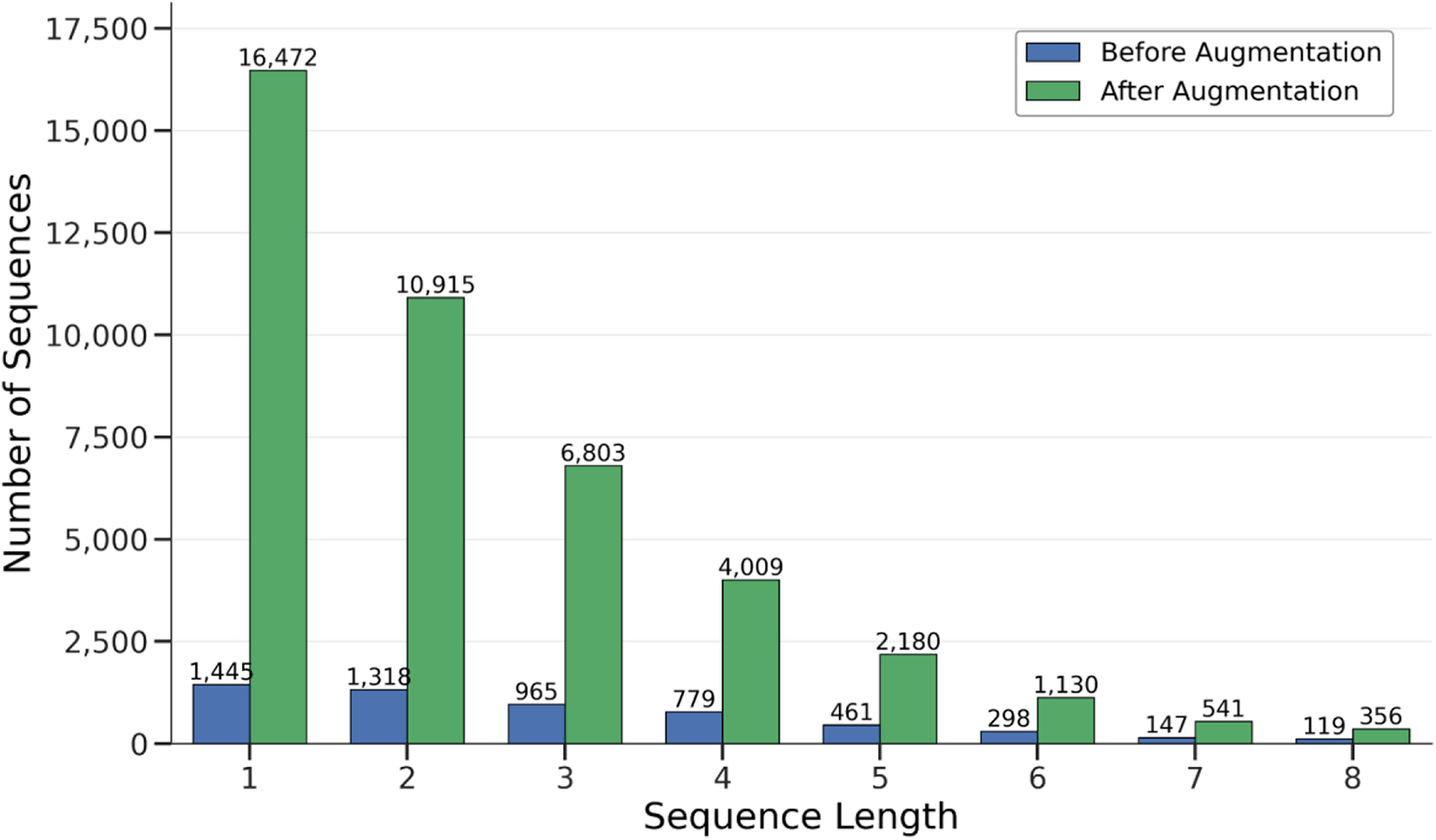
where 0 = (0, 0) denotes the padding token. This augmentation ensured that all valid prefixes of S i contributed training examples, enabling models to learn from both complete and partial histories. Figure 1 illustrates the variation in sequence lengths before and after augmentation.
Sequence length distribution pre- and post-augmentation, highlighting the substantial increase in the number of sequences.

For MLP and Cox models serving as baselines, sequences were flattened into independent records. Each cycle was treated as an isolated observation of the form  ${{\boldsymbol{L}}_{i,t}}\, \mapsto {\boldsymbol{D}}{{\boldsymbol{O}}_{_{i,t}}},{\boldsymbol{\,t\,}} = {\boldsymbol{\,}}1,{\boldsymbol{\,}} \ldots ,{\boldsymbol{\,}}{{\boldsymbol{T}}_i}.$ These records were pooled across cows, randomly shuffled and split into training, validation and test sets with the same 85%/5%/10% proportions, without stratification by cow ID.
Methods
In the experiments, an MLP was utilised and trained independently on the records of the reproduction cycle. Two LSTM variants – unidirectional and bidirectional – were also employed. For the LSTM models, the data are structured as sequences formed by stacking the reproduction cycles of a single cow as explained earlier. Additionally, a Cox proportional hazards model was trained to benchmark the proposed models via the concordance index (c-index).
The MLP serves as a non-sequence baseline: a feedforward neural network with fully connected layers and nonlinear activations trained via backpropagation to model non-linear relationships. RNNs process sequential data using an internal state that enables dependencies across time steps. Unlike feedforward networks, RNNs maintain a memory of prior inputs within a sequence, allowing them to model temporal context and interactions. Here, each cow’s reproduction cycles are treated as a sequence; the hypothesis is that RNNs better capture longitudinal patterns to forecast the DO of the current cycle.
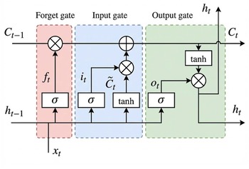
The vanilla RNN (Rumelhart et al., Reference Rumelhart, Hinton, Williams, Anderson and Rosenfeld1988) struggles to learn long-term dependencies due to the vanishing-gradient problem (Pascanu et al., Reference Pascanu, Mikolov and Bengio2012). LSTMs address this limitation and capture longer-term structure in sequences (Hochreiter and Schmidhuber, Reference Hochreiter and Schmidhuber1997). The key mechanism is a memory cell that can store and retrieve information over multiple time steps, selectively retaining essential information while discarding less relevant data. Each LSTM cell (Fig. 2) comprises three gates – input, forget and output – with the following equations:
 \begin{equation}{i_t} = { }\sigma \left( {{W_{\left\{ {xi} \right\}}}{\text{* }}{x_t} + { }{W_{\left\{ {hi} \right\}}}{\text{* }}{h_{\left\{ {t - 1} \right\}}} + { }{b_i}} \right)\end{equation}
An LSTM cell (Jiang et al., Reference Jiang, Chen, Chen, Bo, Li, Tian and Guo2019).

Forget gate:
 \begin{equation}{f_t} = { }\sigma \left( {{W_{\left\{ {xf} \right\}}}{\text{* }}{x_t} + { }{W_{\left\{ {hf} \right\}}}{\text{* }}{h_{\left\{ {t - 1} \right\}}} + { }{b_f}} \right)\end{equation}
Output gate:
 \begin{equation}{o_t} = { }\sigma \left( {{W_{\left\{ {xo} \right\}}}{\text{* }}{x_t} + { }{W_{\left\{ {ho} \right\}}}{\text{* }}{h_{\left\{ {t - 1} \right\}}} + { }{b_o}} \right)\end{equation}
Candidate memory cell:
 \begin{equation}\tau {C_t} = \tanh \left( {{W_{\left\{ {xc} \right\}}}{\text{* }}{x_t} + { }{W_{\left\{ {hc} \right\}}}{\text{* }}{h_{\left\{ {t - 1} \right\}}} + { }{b_c}} \right)\end{equation}
Memory cell:
 \begin{equation}{C_t} = { }{f_t}{\text{* }}{C_{\left\{ {t - 1} \right\}}} + { }{i_t}{\text{* }}\tau {C_t}\end{equation}
Hidden state:
 \begin{equation}{h_t} = { }{o_t}{\text{*}}\tanh \left( {{C_t}} \right)\end{equation}
where σ denotes the sigmoid activation function, tanh denotes the hyperbolic tangent activation function and W and b represent the weight matrices and bias terms for each gate.
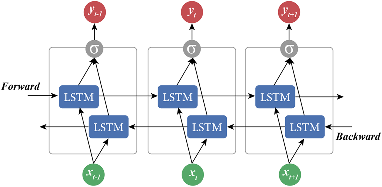
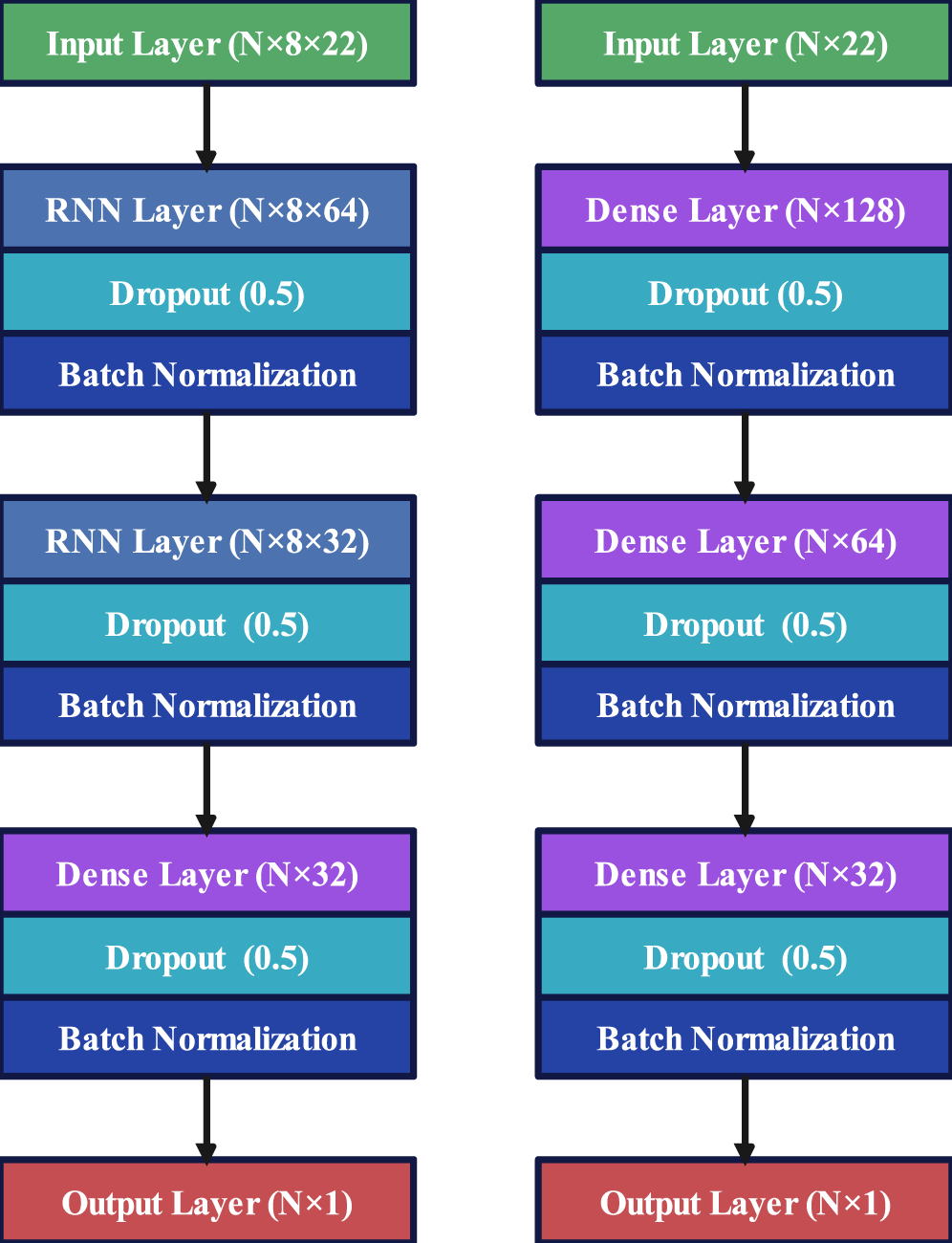
For sequence models, two stacked LSTM layers with 64 and 32 hidden units are used. Dropout (rate 0.5) and batch normalisation are applied to improve generalisation and training stability. The feed-forward baseline comprises two dense layers with 128 and 64 units, respectively, followed by a 32-unit dense layer before the output. All models use the Adam optimiser (learning rate 0.001) and are trained to minimise MAE. Training runs for up to 50 epochs with early stopping based on validation loss; mini-batches of size 64 are used. Sequences are zero-padded to a fixed length of 10 to enable efficient batching. The BiLSTM processes sequences in both directions, integrating past-to-future and future-to-past context within a single representation, which can improve modelling of dependencies spanning multiple cycles (Fig. 3). Figure 4 summarises the final architectures of the LSTM, BiLSTM and MLP models used in this study.
Structure of a bidirectional LSTM (BiLSTM) model.

Final architecture of RNN models (LSTM and BiLSTM) and MLP.

The Cox proportional hazards model is a semi-parametric survival model that accounts for censored data through the hazard function:
 \begin{equation}[{ }h(t{ }|{ }x){ } = { }{h_0}\left( t \right){ } \cdot {\text{exp}}\left( {\beta \cdot x} \right){ }]\end{equation}
where h(t | x) is the hazard function at time t given covariates x, h 0 is the baseline hazard function representing the hazard when all covariates are zero and β are the coefficients associated with the covariates x. As noted, the Cox model is primarily designed to assess the influence of explanatory covariates on event occurrences rather than predict precise event timing; in this work, it is included to benchmark event-ordering via the concordance index, computed solely to assess the relative fitness of the RNN models to the dataset.
Experimental design
To reach the optimal architecture for the neural network models, a systematic hyperparameter tuning procedure (grid search) was conducted. This involved training the models under all candidate configurations and selecting those that minimised validation error. The hyperparameters under tuning included learning rate; optimiser (SGD, Adam [Kingma and Ba, Reference Kingma and Ba2014], RMSprop [Tieleman and Hinton, Reference Tieleman and Hinton2012]); activation functions in dense layers; depth and width of dense layers; and the dimensions of the stacked RNN layers. Final configurations are summarised in the training protocol. After finalising architectures, each model was trained in 10 independent runs with distinct random seeds and re-sampled splits; metrics were computed per run and summarised across runs.
Statistics
To assess and compare model performance in the hyperparameter tuning and the training runs, we employed a set of complementary metrics tailored to capture different aspects of predictive accuracy. MAE measures the average absolute difference between predicted and observed values:
 \begin{equation}MAE = \frac{1}{n}\mathop \sum\nolimits_{i = 1}^n \left| {{y_i} - { }{{\hat y}_i}} \right|\end{equation}
MSE quantifies the average of squared differences between predictions and observations:
 \begin{equation}MSE = \frac{1}{n}\mathop \sum \nolimits_{i = 1}^n {({y_i} - { }{\hat y_i})^2}\end{equation}
The coefficient of determination  $\left( {{R^2}} \right)$ expresses the proportion of variance in the dependent variable explained by the independent variables:
 \begin{equation}{R^2} = \frac{{\mathop \sum \nolimits_{i = 1}^n {{({y_i} - { }{{\hat y}_i})}^2}}}{{\mathop \sum \nolimits_{i = 1}^n {{({y_i} - { }\bar y)}^2}}}\end{equation}
For event-ordering, the concordance index (c-index) evaluates how well the model ranks survival times, a key consideration when some observations may be censored. Although censored data were removed during RNN training to satisfy model requirements, the c-index remains informative for comparisons with traditional survival models. It is defined as:
 \begin{align}
& cindex \nonumber\\
&= \frac{{number \ of \ concordant \ pairs}}{{number \ of \ concordant \ pairs + number \ of \ discordant \ pairs}}\end{align}
where concordant pairs are those for which the model correctly predicts the relative order of survival times and discordant pairs are those for which it does not; the index ranges from 0.5 (random ordering) to 1 (perfect ordering), with higher values indicating better concordance.
In summary, the methodological innovation lies in treating days-open prediction as a sequence-modelling problem under strict temporal validity with leakage-aware evaluation, complemented by a survival benchmark for event-ordering. All predictor summaries (e.g., body/motion scores, milk yield/composition, disorders) are aligned to end at or before the relevant reproductive event to preclude any post-outcome information. Consecutive lactation cycles are encoded as variable-length sequences so longitudinal dependencies – missed by single-record models – can be learned while cow-level splits prevent information leakage across sets. To mirror real-world partial histories, all valid sub-sequences up to length 10 are generated and padded only for batching. Missing values are imputed using a K-nearest-neighbours scheme (K = 10) selected via variable-wise completeness profiling so that multivariate structure is retained. Evaluation reports MAE, MSE, R2 and c-index to compare fairly with survival models and assess ordering, and each model is trained across repeated runs with distinct seeds to quantify stability and avoid optimistic estimates.
From a computational perspective, one-time preprocessing dominates in KNN imputation, which in the worst case requires  $O({N^2}D)$ distance computations (N samples, D features), followed by linear-time outlier handling
 $O\left( {ND} \right)$. Sequence augmentation grows the number of training examples linearly in the number of valid sub-sequences and does not change the asymptotic complexity. For learning, an LSTM with two stacked layers of sizes
 ${H_1}$ and
 ${H_2}$ over sequences of length
 $L$ has per-epoch cost
 $O(\sum\nolimits_i {{L_i}(D {H_1} + {H_1}^2 + {H_1}{\kern 1pt} \;{H_2} + {H_2}^2)} )$ across sequences i, with memory proportional to
 $O(L\;({H_1} + {H_2}))$ per batch due to back-propagation through time. The MLP baseline incurs
 $O(N\;D\;H + {H^2}))$ per epoch, while the Cox model typically involves iterative optimisation with per-iteration cost on the order of
 $O(N\;D + {D^2})$. Inference is linear in sequence length for the LSTM,
 $O(L\;(D\;{H_1}^2 + {H_1}\;{H_2} + {H_2}^2))$ and constant in L for the MLP and Cox models. In practice for this dataset (L ≤ 10, D ≈ 20–30, moderate H), training is tractable on a single modern CPU/GPU and inference is fast enough for herd-level deployment.
Results
This study conducted a controlled experiment utilising three deep learning models: MLP, LSTM and BiLSTM, in conjunction with the Cox proportional hazards model. To reach an efficient structure for each model, a systematic hyperparameter tuning process was conducted as explained earlier. Figure 4 illustrates the ultimate architecture for each model after the tuning process. The RNN model, which includes LSTM and BiLSTM variants, starts with an input layer that accepts sequences of length 10, each with 22 features. This is followed by two RNN layers with 64 and 32 nodes, respectively. Each RNN layer includes a dropout rate of 0.5 and batch normalisation. The MLP model begins with an input layer that accepts 22 features. This leads to two dense layers with 128 and 64 nodes, respectively. Similar to the RNN model, each layer includes a dropout rate of 0.5 and batch normalisation. Both models converge into a dense layer with 32 nodes, followed by dropout and batch normalisation, before reaching the output layer. For the dense layers, the rectified linear unit (ReLU) activation function was used. The Adam algorithm, with a learning rate of 0.001, was used for weight optimisation.
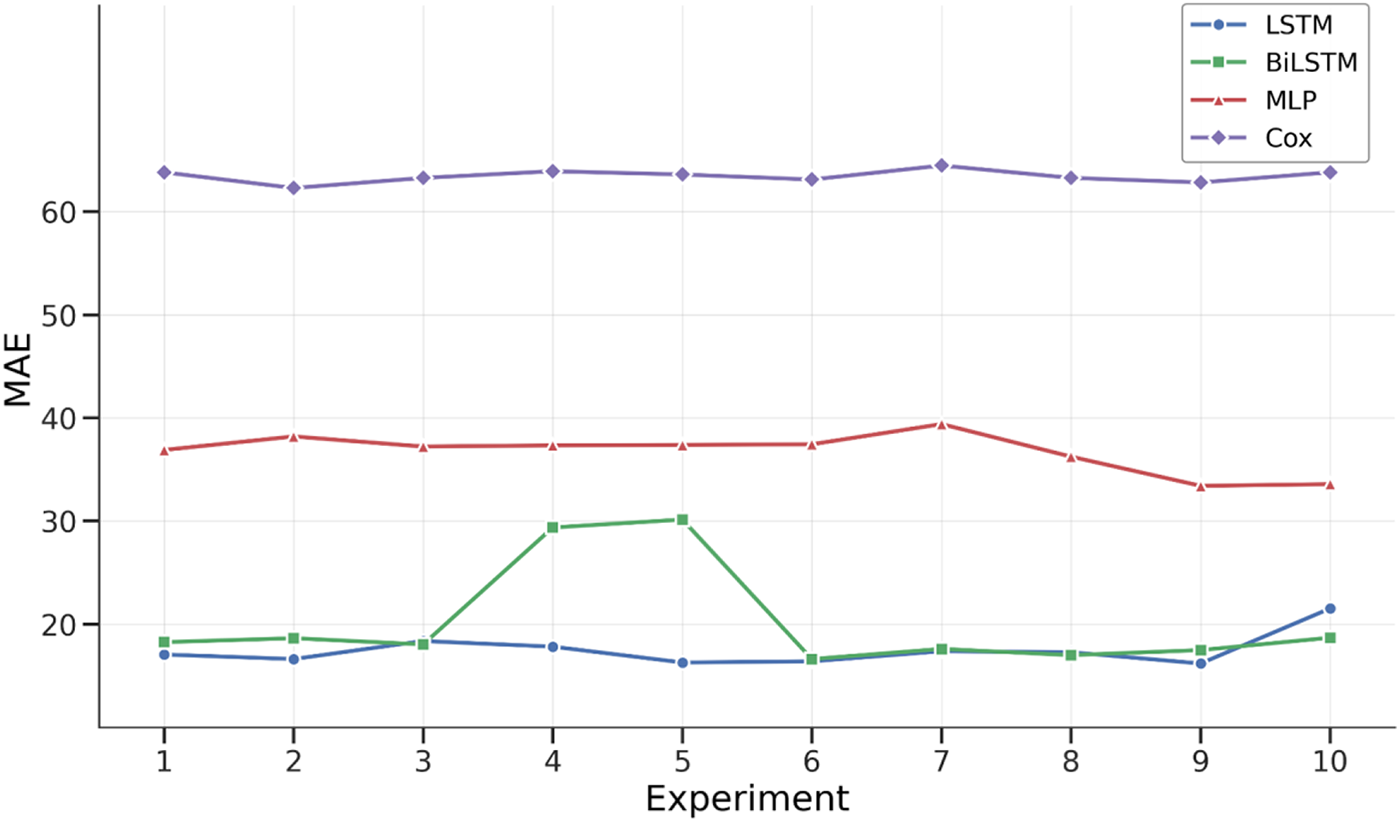
Upon finalising the optimal architectures, training experiments were initiated by fitting the models to the prepared datasets. To bolster the robustness and reliability of the results, 10 iterations were executed encompassing random shuffling, data splitting, sequence generation and training, each with a unique initialisation of model weights. For every training iteration, the specified evaluation metrics were computed and the results recorded. The consolidated outcomes of this process are encapsulated in Table 2, which displays the evaluated metrics derived from the mean values across all iterations. Furthermore, Figure 5 shows the value of MAE across 10 training runs.
Comparison of mean absolute error (MAE) for different models over 10 training runs, each initiated with distinct random weights and different shuffling of data splits.

Average of evaluation metrics for 10 training runs

The experimental findings reveal that the RNN models, specifically LSTM and BiLSTM, significantly improved prediction accuracy compared to the MLP and Cox models. The LSTM model, with its architecture of two consecutive RNN layers, reduced the MAE by approximately half compared to the MLP model, which consists only of densely connected layers. While the LSTM model demonstrated the best performance across all metrics on average over the 10 training runs, it is noteworthy that the BiLSTM model slightly outperformed the LSTM model in some of the experimental iterations (3, 8 and 10).
In terms of event concordance, the Cox model, despite outperforming the MLP model with a rate of nearly 67%, was still surpassed by the RNN models. This aligns with the inherent strength of the Cox model as a semi-parametric model, adept at accurately forecasting chronological sequences of events, albeit with limited precision in pinpointing their exact timing. However, the RNN models’ superior performance in terms of concordance underscores the formidable capacity of deep neural networks to capture intricate trends in the data, thereby surpassing the capabilities of conventional statistical models in survival analysis.
Regarding stability, the models exhibit a moderate level of consistency across the multiple experimental runs, as evidenced by their MAE scores (Fig. 5). The LSTM model, along with the MLP and Cox models, shows relatively subtle differences in the amount of error. However, the BiLSTM model exhibits a slightly higher variation in the amount of error, which leads to it occasionally outperforming and at other times underperforming compared to the unidirectional LSTM model. Despite these fluctuations, the LSTM model emerges as the most reliable performer overall.
In a comparative assessment of RNN models’ predictive performance across varying reproductive conditions, distinct patterns were observed in the MAE values for sequences concluding with either a healthy or diseased cycle. The LSTM model demonstrated an MAE of approximately 18.42 for sequences ending in a diseased reproductive cycle, compared to 17.20 for those concluding in a healthy cycle. This represents an average increase of roughly 7.10% in MAE when predicting sequences concluding in a diseased reproductive cycle. Similarly, the BiLSTM model showed an MAE of about 21.76 for diseased sequences and 19.58 for healthy sequences, indicating an average increase of approximately 11.13% in MAE for sequences ending in a diseased cycle. These findings highlight the models’ sensitivity to the concluding condition of the reproductive cycle, with a noticeable increase in error rates when predicting diseased outcomes.
Discussion
The results indicate that sequence models capture structure in longitudinal reproductive histories that point-in-time models miss. Improvements over the feed-forward baseline and the survival model are consistent across runs, supporting the view that temporal dependencies between consecutive cycles carry predictive signal beyond static covariates and proportional-hazards assumptions. Directionality appears less critical: the unidirectional LSTM is consistently strong, while the bidirectional variant yields marginal, context-dependent gains, suggesting that most of the useful information is contained in the past trajectory rather than requiring future context within the sequence.
From a practical standpoint, the absolute error is moderate relative to the distribution of DO (with a population mean near 150 days). This magnitude can support herd-level management (e.g., identifying animals at higher risk of prolonged intervals) but may be insufficient for individual-level scheduling where week-level precision is required. Error inflation observed for sequences concluding with disease aligns with expectations: health events introduce variability in physiological recovery and management interventions, which reduces predictability. This pattern highlights the value of incorporating richer, time-localised health representations and potentially time-varying covariates.
Data quality likely constrained performance. Several high-value predictors exhibit substantial missingness (e.g., milk composition and motion scores), necessitating imputation. While KNN preserves multivariate structure better than single-value fills, the high proportion of missing values in specific variables limits the information available to the models and may attenuate potential gains. Moreover, although outliers were handled and temporal validity enforced during preprocessing, the single-farm setting and long study horizon raise questions about shifts in management practices, recording protocols and genetics that the current models do not explicitly account for.
Generalisability remains an open question. Splitting by cow mitigates leakage, and repeated training runs show stable rankings; however, external evaluation on independent farms and periods is needed to assess transportability. Additionally, the comparison with the Cox model should be interpreted as a ranking sanity check rather than a like-for-like alternative, given differences in handling censored data and model objectives.
Taken together, the findings support sequence-based modelling as a principled approach for forecasting DO. The models are robust across runs and more aligned with the temporal nature of the problem than static baselines, yet their utility would likely increase with higher-fidelity longitudinal predictors, explicit handling of censoring and external validation.
Conclusion
This study explored predictive models for DO in dairy cattle, a critical metric impacting both the economic and animal welfare facets of dairy farming. Employing an approach based on machine learning and deep neural networks, the objective was to equip dairy farmers with precise tools for refining breeding practices and enhancing herd management. By discerning the temporal patterns inherent in cows’ reproductive cycles, the capabilities of RNN models were leveraged. The findings demonstrated their potential in enhancing prediction accuracy, reducing the error by approximately half. This represents a first step towards predicting DO using data mining methods and, despite its challenges, serves as a testament to the potential of advanced time-series deep learning models for DO prediction in dairy cattle. These models, with further refinement, data collection and research, could provide dairy farmers with precise tools to fine-tune breeding strategies, optimise herd management and bolster both the economic sustainability and the welfare of animals in dairy farming.
Limitations and future work
The dataset originates from a single commercial farm over a long horizon, which may embed shifts in management, genetics and recording practices; external validation across herds and time is needed to assess transportability. Several potentially informative predictors (e.g., milk composition, motion scores) exhibit substantial missingness; richer, more frequent measurements could strengthen sequence signals and reduce reliance on imputation. The current formulation does not explicitly model censoring, and the comparison to the Cox model focuses on ranking rather than a censored regression objective; extending sequence models to handle censored outcomes directly would offer a more rigorous benchmark. Finally, modelling choices such as fixed-length padding and summary-level features could be relaxed by moving to time-varying covariates, attention mechanisms and irregular-time sequence models, which may yield further gains.
Competing interests
The authors declare no competing interests.