1 Introduction
In this article, we discuss the classification problem of automorphism groups of K3 surfaces over
 $\mathbb {C}$
.
There are two approaches to automorphisms of K3 surfaces. The first one is the classification under some finiteness conditions, such as the classification of finite subgroups, and that of possible finite order of automorphisms. For example, a well-known and important result in this approach is Mukai’s result [Reference Mukai15] Theorem (0.3), which says that symplectic finite subgroups of the automorphism groups of K3 surfaces are isomorphic to subgroups of the Mathieu group
 $M_{23}$
, one of the sporadic simple groups.
The other approach is the application of Borcherds’ Lattice Theory (often called Borcherds’ method) to compute a generating set of infinite automorphism groups. The problem of finding a generating set of the automorphism groups of Kummer surfaces was first proposed by Klein. This problem took more than 100 years to be solved by Kondo [Reference Kondo13] using Borcherds’ method. Although this method is very useful and, in fact, the automorphism groups of some specific K3 surfaces have been calculated, this method is not applicable to the general case.
Shigeru Mukai recently proposed at the occasion of the Algebra Symposium in Tokyo in 2018, the following conjecture on discrete group theory and automorphism groups, from which one may hopefully find a general framework for dealing with infinite automorphism groups of elliptic K3 surfaces.
Conjecture 1. Let X be an elliptic K3, Enriques or Coble surface, and let
 $\operatorname {Aut}(X)$
be the automorphism group of X. Then, the virtual cohomological dimension
 $\operatorname {vcd}(\operatorname {Aut}(X))$
of
 $\operatorname {Aut}(X)$
is equal to the maximum of the Mordell–Weil rank induced by all elliptic surface structures on X (for the definition of the virtual cohomological dimension of a group, see Definitions 4.3 and 4.5).
Remark 1.1. The virtual cohomological dimension of
 $\operatorname {Aut}(X)$
is easily seen to be larger than the rank of the Mordell–Weil group of any elliptic fibration. Hence, the main point of Mukai’s conjecture lies in finding the upper bound of
 $\operatorname {vcd}(\operatorname {Aut}(X))$
as stated therein.
This conjecture could be a turning point from the conventional study of automorphism groups of elliptic K3, Enriques and Coble surfaces by computing their generators to that by computing their cohomological invariants. Our main result is a formula which determines the virtual cohomological dimension of the automorphism group of a K3 surface by the covering dimension of the blown-up boundary associated with the ample cone of the K3 surface (for the definitions of covering dimension and blown-up boundary, see Definitions 4.6 and 5.27, respectively).
Theorem 1. Let X be an algebraic K3 surface with its Picard rank
 $\rho (X)\geq 3$
. If the symplectic automorphism group
 $\operatorname {Aut}_{s}(X)$
of X is non-elementary, then
 $$\begin{align*}\operatorname{vcd}(\operatorname{Aut}(X)) = \dim \partial A_{X}^{bl} + 1,\end{align*}$$
where
 $\partial A_{X}^{bl}$
is the blown-up boundary associated with the ample cone of X (see Theorem 5.35 for the detailed discussion).
To show this result, we focus on the natural action of automorphism groups on hyperbolic spaces, which comes from the action on the cohomology of degree 2. Then, we can consider the symplectic automorphism group of a K3 surface as a discrete subgroup of Möbius transformations of a hyperbolic space. Moreover, we can show the following theorem.
Theorem 2. Let X be an algebraic K3 surface with
 $\rho (X)\geq 3$
, and let
 $\operatorname {Aut}_{s}(X)$
be the symplectic automorphism group of X. Then,
 $\operatorname {Aut}_{s}(X)$
is geometrically finite (for the definition of geometrically finite groups, see Definition 3.29).
Bestvina and Mess [Reference Bestvina and Mess5] showed that the cohomological dimension of a torsion-free hyperbolic group is determined by the covering dimension of its Gromov boundary. Recently, Tomohiro Fukaya [Reference Fukaya10] generalized the formula for relatively hyperbolic groups satisfying a certain condition. Geometrically finite groups are typical examples of relative hyperbolic groups. We can immediately obtain Theorem 1 by applying Fukaya’s result [Reference Fukaya10, Corollary B].
On the other hand, the paper of Fukaya is still unpublished at the time when the first draft of this article was written, and his theorem and his proof are stated using geometric group theory. For readability to algebraic geometers, this article also contains the result and the proof of Fukaya, which are simplified and modified to fit in with our situation, in §5.2, using the geometry of ample cones of K3 surfaces and hyperbolic geometry.
Remark 1.2. After the author finished the first draft of this article, Tomohiro Fukaya informed the author that Theorem 2 has been independently obtained and proved by Kohei Kikuta. He showed geometrical finiteness for the automorphism groups of irreducible symplectic varieties over a field of characteristic zero, and his proof is different in some points from our proof given in this article. For more details, the reader is advised to refer to his paper [Reference Kikuta12].
An application of Theorem 1 is the case that the ample cones of K3 surfaces are sphere packings (see Definition 5.39 for sphere packings).
Theorem 3. Let X be an algebraic elliptic K3 surface with
 $\rho (X) \geq 3$
. If
 $\partial A_{X}$
is a connected sphere packing, and every elliptic divisor of X corresponds to the tangent point of some two spheres associated with
 $(-2)$
-curves, then
 $$\begin{align*}\operatorname{vcd}(\operatorname{Aut}(X)) =\max \{ \operatorname{rk}\operatorname{MW}(f)\} =\rho(X)-3 ,\end{align*}$$
where f runs all elliptic fibrations of X and
 $\operatorname {rk}\operatorname {MW}(f)$
is the rank of the Mordell–Weil group
 $\mathrm {MW}(f)$
associated with f.
Baragar [Reference Baragar2] constructed K3 surfaces whose ample cones are sphere packings. Then, we can compute the virtual cohomological dimension of their automorphism groups. Note that these K3 surfaces provide examples that affirm Conjecture 1, and, to the best of our knowledge, they are the first non-trivial examples in the sense that the verification of the conjecture does not rely on explicit calculation of the group structure of the automorphism groups.
Finally, using hyperbolic geometry, we construct counterexamples to Mukai’s conjecture for elliptic K3 surfaces. These examples have the property that the virtual cohomological dimension of their automorphism group is one, while the rank of the Mordell–Weil group is zero for every elliptic fibration. For details, see the §6.2.
2 Lattices and K3 surfaces
In this section, we recall some definitions and facts about lattices and K3 surfaces.
2.1 Lattices
Let L be a free abelian group of rank r, and let
 $\langle \hspace {2mm}, \hspace {2mm} \rangle : L \times L\rightarrow \mathbb {Z}$
be a symmetric bilinear form. A symmetric bilinear form
 $\langle \hspace {2mm}, \hspace {2mm} \rangle $
is said to be non-degenerate if
 $\langle x, y \rangle = 0,$
for any
 $y \in L$
implies
 $x=0$
. We call a pair
 $(L, \langle \hspace {2mm}, \hspace {2mm} \rangle )$
of L and a non-degenerate symmetric bilinear form a lattice of rank r. The dual
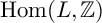 $\operatorname {Hom}(L, \mathbb {Z})$
is denoted by
 $L^{*}.$
Since L is non-degenerate, the natural map
 $$ \begin{align} L \rightarrow L^{*}, x \mapsto f_{x} \end{align} $$
is injective, where
 $f_{x}$
is the linear function on L defined by
 A lattice L is said to be unimodular if the natural map (2.1) is an isomorphism. A lattice L is said to be even if
 $\langle x, x \rangle $
is an even integer for any
 $x\in L$
. For an even lattice L, the quotient group
 $L^{*}/L$
is denoted by
 $A_{L}$
. An element x of L with
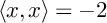 $\langle x, x \rangle =-2$
is called a root of L.
A subgroup S of a lattice L is called a sublattice of L if S with the restriction of the bilinear form of L is a lattice. A sublattice S of L is said to be primitive if the quotient group
 $L/S$
is torsion-free. The orthogonal complement of a sublattice S, denoted by
 $S^{\bot }$
, is a primitive sublattice of L.
An isomorphism from L to itself is called an automorphism of L. The set of automorphisms of L is called the orthogonal group of L, and it is denoted by
 $O(L).$
2.2 K3 surfaces
Theorem 2.1 [Reference Kondo14, Theorem 4.5]
For a K3 surface X, the second cohomology group
 $H^{2}(X,\mathbb {Z})$
with the cup product is a unimodular even lattice with the signature
 $(3,19)$
. Then,
 $H^{2}(X,\mathbb {Z})$
is isomorphic to
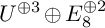 $U^{\oplus 3}\oplus E_{8}^{\oplus 2}$
, where U is the hyperbolic lattice of rank 2.
Definition 2.2. Let
 $\omega _{X}$
be a nowhere vanishing holomorphic
 $2$
-form of X. The Néron–Severi lattice
 $\operatorname {NS}(X)$
is defined by

The Néron–Severi lattice
 $\operatorname {NS}(X)$
is a lattice by the cup product of signature
 $(1, \rho (X)-1)$
, where
 $\rho (X)$
is the Picard number of X. The transcendental lattice
 $T_{X}$
of X is defined by
 $\operatorname {NS}(X)^{\bot }$
.
Definition 2.3. Let X be a K3 surface. We define

and

For
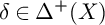 $\delta \in \Delta ^{+}(X)$
, the reflection
 $s_{\delta }$
in
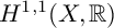 $H^{1,1}(X, \mathbb {R})$
is defined by
 $$\begin{align*}s_{\delta}(x)=x+ \langle x,\delta \rangle \delta \hspace{2mm}for \hspace{2mm} x\in H^{1,1}(X, \mathbb{R})\end{align*}$$
The reflection group
 $W(X)$
is the subgroup of
 $O(H^{1,1}(X, \mathbb {R}))$
generated by the set of reflections
 $\{ s_{\delta } : \delta \in \Delta (X) \rbrace .$
The cone
 $P(X)= \lbrace x \in H^{1,1}(X, \mathbb {R}) : \langle x, x \rangle> 0 \rbrace $
has two connected components and the one containing the Kähler class is denoted by
 $P^{+}(X)$
and called the positive cone.
Definition 2.4. The group
 $W(X)$
acts on the space
 $P^{+}(X)$
in a canonical way. The Kähler cone of X is the one of the fundamental domains of
 $W(X)$
given by
 $$\begin{align*}D(X) = \lbrace x \in P^{+}(X) : \langle x, \delta \rangle> 0 {\text{ for any }}\delta \in \Delta^{+}(X) \rbrace. \end{align*}$$
Definition 2.5. Let X be an algebraic K3 surface. The ample cone
 $A(X)$
is defined to be
 $$\begin{align*}A(X) = \lbrace x \in \operatorname{NS}(X) \otimes \mathbb{R} \cap P^{+}(X) : \langle x, \delta \rangle> 0 {\text{ for any }}\delta \in \Delta^{+}(X)\rbrace.\end{align*}$$
Let
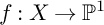 $f :X \to \mathbb {P}^{1}$
be an elliptic fibration of a K3 surface X, and let
 $j:J\rightarrow \mathbb {P}^{1}$
be the jacobian fibration of f. The sections of j generate a group
 $MW(f)$
that is called the Mordell–Weil group of the elliptic fibration
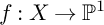 $f :X \to \mathbb {P}^{1}$
. The Mordell–Weil group
 $MW(f)$
is a finitely generated abelian group. We denote by
 $r(f)$
the rank of
 $MW(f)$
.
The following formula is called Shioda–Tate formula.
Lemma 2.6. [[Reference Shioda18], Formula (5.10); Reference Cossec, Dolgachev and Liedtke9, Formula (4.3.2)] Let
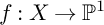 $f:X\to \mathbb {P}^{1}$
be an elliptic fibration of a K3 surface, and let
 $F_{v}=f^{-1}(t_{v}) \; (1\leq v \leq k)$
be the singular fibres of f. We denote by
 $m_{v}$
the number of irreducible components of
 $F_{v}$
. Then, the
 $r(f)$
is given by the following formula:
 $$\begin{align*}r(f)= \rho(X)-2-\sum_{v=1}^k (m_{v}-1).\end{align*}$$
3 Hyperbolic geometry
In this section, we recall some basic facts of n-dimensional hyperbolic spaces and discrete groups of isometries of n-dimensional hyperbolic spaces, which are contained in [Reference Ratcliffe17].
Notation
Let
 $(X, d)$
be a metric space, and let r be a positive real number. Throughout this section, we denote by:
 $B(a, r)$
the open ball of radius r centered at a point a of X;
 $C(a, r)$
the closed ball of radius r centered at a point a of X;
 $S(a, r)$
the sphere of radius r centerd at a point a of X;
 $N(S, r)$
the r-neighborhood of a subset S of X;
 $I(X)$
the group of isometries of X.
We denote by
 $S^{n}$
the n-dimensional unit sphere of
 $\mathbb {R}^{n+1}$
. A vector
 $e_{i}$
in
 $\mathbb {R}^{n}$
is the vector whose i-th entry is 1 and the other entries are
 $0$
.
In hyperbolic geometry, it is useful to use some models of hyperbolic spaces for different situations. Therefore, we begin with recalling the hyperboloid model of hyperbolic spaces. In §3.3 and §3.4 we recall the conformal ball model, and the upper half-space model of hyperbolic spaces.
3.1 The hyperboloid model
Definition 3.1. Let n be a non-negative integer. Let
 $x=(x_{1}, \ldots , x_{n}, x_{n+1})$
and
 $y=(y_{1}, \ldots , y_{n}, y_{n+1})$
be vectors in the
 $(n+1)$
-dimensional real vector space
 $\mathbb {R}^{n+1}$
. The Lorentzian inner product of x and y is defined by
 $$\begin{align*}x\circ y = x_{1}y_{1}+ \cdots +x_{n}y_{n} -x_{n+1}y_{n+1}.\end{align*}$$
The Lorentzian (n+1)-space is the vector space
 $\mathbb {R}^{n+1}$
together with the Lorentzian inner product. A real
 $(n+1)\times (n+1)$
matrix A is said to be Lorentzian if for any
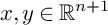 $x, y\in \mathbb {R}^{n+1}$
,
 $x \circ y = Ax \circ Ay.$
Definition 3.2. The hyperboloid model
 $H^{n}$
of hyperbolic n-spaces is defined to be the set
 $\{ x \in \mathbb {R}^{n+1} : x\circ x = -1,\hspace {1mm} x_{n+1}>0 \}.$
The hyperbolic distance
 $d_{H}(x, y)$
between x and y is defined by the equation
 $$\begin{align*}\cosh d_{H}(x, y) = -x\circ y.\end{align*}$$
By [Reference Ratcliffe17, Theorem 3.2.2], the hyperbolic distance
 $d_{H}$
is a metric on
 $H^{n}$
. By the definition of
 $d_{H}$
, Lorentzian
 $(n+1)\times (n+1)$
matrices naturally act isometrically on
 $H^{n}$
. We denote the group of isometries by
 $I(H^{n}).$
Definition 3.3. Let
 $H^{n}$
be the hyperboloid model of n-dimensional hyperbolic spaces. The set of all Lorentzian
 $(n+1)\times (n+1)$
matrices with matrix multiplication is called the Lorentz group of
 $(n+1) \times (n+1)$
matrices, and is denoted by
 $O(n, 1)$
. The positive Lorentz group
 $O^{+}(n, 1)$
is defined by
 $$\begin{align*}O^{+}(n, 1) = \{ A \in O(n, 1) : AH^{n} = H^{n} \}.\end{align*}$$
By [Reference Ratcliffe17, Theorem 3.2.3], there is an isomorphism from the positive Lorentz group
 $O^{+}(n,1)$
to the group of hyperbolic isometries
 $I(H^{n})$
.
Definition 3.4. A hyperbolic m-plane of
 $H^{n}$
is the nonempty intersection of
 $H^{n}$
with an
 $(m+1)$
-dimensional vector subspace of
 $\mathbb {R}^{n+1}$
.
3.2 Möbius transformations
To define the conformal ball model and the upper half-space model of hyperbolic n-spaces, we use the hyperboloid model and Möbius transformation. In this section, we recall the definition and some basic facts of Möbius transformation.
Definition 3.5. Let
 $E^n$
be an n-dimensional Euclidean space. Let a be a unit vector in
 $E^{n}$
, and let t be a positive real number. Consider the hyperplane of
 $E^{n}$
is defined by
 $$\begin{align*}P(a, t) = \{x \in E^{n} : a\cdot x = t\},\end{align*}$$
where
 $a\cdot x$
is the Euclidean inner product of a and x. The reflection
 $\rho $
of
 $E^{n}$
in the plane
 $P(a, t)$
is defined by
 $$\begin{align*}\rho(x) = x + 2(t-a\cdot x)a.\end{align*}$$
Let a be a point in
 $E^{n}$
, and let r be a positive real number. The sphere of
 $E^{n}$
of radius r centered at a is defined by
 $$\begin{align*}S(a, r) = \{x \in E^{n}: |x-a| = r\},\end{align*}$$
where
 $|x-a|$
is the Euclidean norm of
 $x-a$
. The reflection (or inversion)
 $\sigma $
of
 $E^{n}$
in the sphere
 $S(a, r)$
is defined by
 $$\begin{align*}\sigma (x) = a + \bigg(\frac{r}{|x-a|}\bigg)^{2} (x-a).\end{align*}$$
Let
 $\infty $
be a point not in
 $E^{n}$
. We define
 $\hat {E}^{n}=E^{n}\cup \{\infty \}$
whose topology is given by the one-point compactification of
 $E^n$
.
Definition 3.6. Let a be a unit vector in
 $E^{n}$
, and let t be a positive real number. The extended hyperplane of
 $\hat {E}^{n}$
is defined by
 $\hat {P}(a, t) = P(a, t)\cup \{\infty \}.$
Let
 $\rho $
be the reflection of the hyperplane
 $P(a, t)$
. Extend
 $\rho $
to a bijection
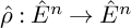 $\hat {\rho }: \hat {E}^{n} \rightarrow \hat {E}^{n}$
by setting
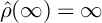 $\hat {\rho }(\infty ) = \infty $
. In a similar way, the inversion
 $\sigma $
of a Euclidean sphere
 $S(a, r)$
in
 $E^{n}$
is extended to
 $\hat {\sigma }:\hat {E}^{n} \rightarrow \hat {E}^{n}$
by setting
 $\hat {\sigma }(\infty ) = a$
and
 $\hat {\sigma }(a)=\infty .$
The extended map
 $\hat {\rho }$
(resp.
 $\hat {\sigma }$
) is called the reflection of
 $\hat {P}(a, t)$
(resp.
 $\hat {S}(a, r)$
), which is a homeomorphism of
 $\hat {E}^{n}$
.
Definition 3.7. A sphere of
 $\hat {E}^{n}$
is either an extended hyperplane or a Euclidean sphere. A Möbius transformation of
 $\hat {E}^{n}$
is a finite composition of reflections of
 $\hat {E}^{n}$
in spheres.
3.3 The conformal ball model
In this section, we recall the conformal ball model of hyperbolic space. Identify
 $\mathbb {R}^{n}$
with
 $\mathbb {R}^{n} \times \{0\}$
in
 $\mathbb {R}^{n+1}$
. Let
 $B^{n}$
be the open unit ball of
 $\mathbb {R}^{n},$
and let
 $|x|$
be the Euclidean norm of a vector x in
 $\mathbb {R}^{n}$
: that is,
 $|x|= (x_{1}^{2}+\cdots +x_{n}^{2})^{\frac {1}{2}}.$
The stereographic projection
 $\zeta $
from
 $B^{n}$
to the hyperbolic space
 $H^{n}$
is defined by the formula
 $$\begin{align*}\zeta (x) = \Big( \hspace{0.5mm} \frac{2x_{1}}{1-|x|^{2}}, \ldots, \frac{2x_{n}}{1-|x|^{2}},\frac{1+|x|^{2}}{1-|x|^{2}} \hspace{0.5mm}\Big).\end{align*}$$
This map
 $\zeta $
is bijective.
Definition 3.8. A metric
 $d_{B}$
on
 $B^{n}$
is defined by the formula
 $d_{B}(x, y)= d_{H}(\zeta (x), \zeta (y)).$
The metric space
 $(B^{n}, d_{B})$
is called the conformal ball model of hyperbolic n-spaces.
Definition 3.9. A Möbius transformation of
 $B^{n}$
is a Möbius transformation
 $\phi $
of
 $\hat {E}^{n}$
that leaves
 $B^{n}$
invariant: that is,
 $\phi $
satisfies
 $\phi (B^{n}) = B^{n}.$
The group of Möbius transformations of
 $B^{n}$
is denoted by
 $M(B^{n})$
.
It is well-known that every Möbius transformation of
 $B^n$
restricts to an isometry of the conformal ball model
 $B^n$
and the restriction induces an isomorphism from
 $M(B^n)$
to
 $I(B^n).$
The boundary of
 $B^{n}$
in
 $\mathbb {R}^{n}$
, denoted by
 $\partial B^{n}$
, is the unit sphere
 $\{ x \in \mathbb {R}^{n} : |x|=1 \}.$
A hyperbolic m-plane of
 $B^{n}$
is the image of a hyperbolic m-plane of
 $H^{n}$
by
 $\zeta ^{-1}$
. By [Reference Ratcliffe17, Theorem 4.5.3], a hyperbolic m-plane of
 $B^{n}$
is the intersection of
 $B^{n}$
with either an m-dimensional vector subspace of
 $\mathbb {R}^{n}$
or an m-dimensional sphere of
 $\mathbb {R}^{n}$
orthogonal to
 $\partial B^{n}.$
Definition 3.10. Let c be a point in
 $\partial B^{n}$
. Let S be an
 $(n-1)$
-dimensional inscribed sphere of
 $B^{n}$
tangent at c, and let T be the one of connected components of
 $\mathbb {R}^{n}\backslash S$
which is bounded. We call the intersection of
 $B^{n}$
with S (resp. T) a horosphere of
 $B^{n}$
(resp. a horoball of
 $B^{n}$
).
3.4 The upper half-space model
Definition 3.11. Let
 $x=(x_{1}, \ldots , x_{n})$
be a vector in
 $\mathbb {R}^{n}$
, and let
 $e_{n}$
be the vector in
 $\mathbb {R}^{n}$
whose entries are all zero except for the n-th, which is one. Let
 $\rho $
(resp.
 $\sigma $
) be the reflection of
 $\hat {E}^{n}$
in
 $P(e_{n}, 0)$
(resp.
 $S(e_{n}, \sqrt {2})$
). The maps
 $\rho $
and
 $\sigma $
is given by the formula
 $$ \begin{align*} \rho (x) &= (x_{1}, \ldots,x_{n-1}, -x_{n}),\\ \sigma (x) &= e_{n} + \frac{2(x-e_{n})}{|x-e_{n}|^{2}} \text{ for }x \in \mathbb{R}^{n}\backslash \{e_{n}\}. \end{align*} $$
The n-dimensional upper half-space
 $U^{n}$
is defined to be
 $$\begin{align*}U^{n}=\{ (x_{1}, \ldots, x_{n}) \in \mathbb{R}^{n} : x_{n}>0 \}.\end{align*}$$
Then, the map
 $\eta = \sigma \rho $
is a map from the upper half-space
 $U^{n}$
to the open unit ball
 $B^{n}$
, and is called the standard transformation from
 $U^{n}$
to
 $B^{n}.$
The Poincaré metric on
 $U^{n}$
is defined by
 $$\begin{align*}d_{U}(x, y) = d_{B}(\eta (x), \eta (y)).\end{align*}$$
The pair
 $(U^{n}, d_{U})$
is a metric space, and is called the upper half-model of hyperbolic n-spaces. By the definition, this is isomorphic to the conformal ball model
 $B^{n}$
of hyperbolic n-spaces. The group of isometries of
 $U^{n}$
is denoted by
 $I(U^{n})$
.
Definition 3.12. A Möbius transformation of
 $U^{n}$
is a Möbius transformation
 $\phi $
that leaves
 $U^{n}$
invariant: that is,
 $\phi $
satisfies
 $\phi (U^{n}) = U^{n}.$
The group of Möbius transformations of
 $U^{n}$
is denoted by
 $M(U^{n}).$
Every Möbius transformation of the upper half-space model
 $U^{n}$
restricts to an isometry of
 $U^{n}$
and the restriction induces an isomorphism from
 $M(U^{n})$
to
 $I(U^{n}).$
Definition 3.13. Identify
 $E^{n-1}$
with
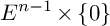 $E^{n-1}\times \{0\}$
in
 $E^{n}.$
Let
 $\phi $
be a Möbius transformation of
 $\hat {E}^{n-1}$
, and let
 $\overline {a} = (a, 0)$
. The extension
 $\overline {\phi }$
of
 $\phi $
is defined as follows:
-
(1) If
 $\phi $
is the reflection of
$\hat {E}^{n-1}$
in
$P(a, t)$
, then
$\overline {\phi }$
is the reflection of
$\hat {E}^{n}$
in
$P(\overline {a}, t)$
.
-
(2) If
$\phi $
is the reflection of
$\hat {E}^{n-1}$
in
$S(a, t)$
, then
$\overline {\phi }$
is the reflection of
$\hat {E}^{n}$
in
$S(\overline {a}, t)$
. -
(3) In the general case,
$\phi $
is the composition
$\phi = \sigma _{1}\cdots \sigma _{m}$
of reflections. Then, we define the map
$\overline {\phi }$
by the composition
$\overline {\phi } = \overline {\sigma _{1}} \cdots \overline {\sigma _{m}}.$





We call the extension of
 $\phi $
the Poincaré extension.
Poincaré extension is well-defined. Moreover, the following holds.
Theorem 3.14 [Reference Ratcliffe17, Theorem 4.4.1]
A Möbius transformation
 $\phi $
of
 $\hat {E}^{n}$
leaves
 $U^{n}$
invariant if and only if
 $\phi $
is the Poincaré extension of a Möbius transformation of
 $\hat {E}^{n-1}.$
In particular, Poincaré extension induces the isomorphism from
 $M(\hat {E}^{n-1})$
to
 $M(U^{n})$
.
Definition 3.15. Let
 $\eta $
be the standard transformation from
 $U^{n}$
to
 $B^n$
. A subset P is a hyperbolic m-plane (resp. horosphere, horoball) of
 $U^n$
if the image
 $\eta (P)$
of P by
 $\eta $
is a hyperbolic m-plane (resp. horosphere, horoball) in
 $B^{n}$
.
Theorem 3.16 [Reference Ratcliffe17, Theorems 4.6.3. and 4.6.5.]
-
(1) A subset P of
$U^n$
is a hyperbolic m-plane of
$U^n$
if and only if P is the intersection of
$U^n$
with either an m-plane of
$E^{n}$
orthogonal to
$E^{n-1}$
or an m-sphere of
$E^{n}$
orthogonal to
$E^{n-1}$
. -
(2) A subset
$\Sigma $
of
$U^n$
is a horosphere of
$U^n$
based at a point b of
$\hat {E}^{n-1}$
if and only if
$\Sigma $
is either a Euclidean hyperplane in
$U^{n}$
parallel to
$E^{n-1}$
if
$b=\infty ,$
or the intersection of
$U^n$
with a Euclidean sphere in
$\overline {U}^n$
tangent to
$E^{n-1}$
at b if
$b\neq \infty .$


3.5 Types of transformations and elementary groups
Let
 $B^{n}$
be the conformal ball model of n-dimensional hyperbolic spaces. We write
 $\overline {B^{n}}$
for the closed unit ball
 $B^{n}\cup \partial B^{n}.$
Definition 3.17. Let
 $\phi $
be an element of
 $M(B^{n})$
. Then,
 $\phi $
maps the closed unit ball
 $\overline {B^{n}}$
to itself. By the Brouwer Fixed-Point Theorem,
 $\phi $
has a fixed point in
 $\overline {B^{n}}$
.
-
(1)
$\phi $
is elliptic if
$\phi $
has a fixed point in
$B^{n}$
; -
(2)
$\phi $
is parabolic if
$\phi $
has no fixed point in
$B^{n}$
and has a unique fixed point in
$\partial B^{n}$
; -
(3)
$\phi $
is hyperbolic if
$\phi $
has no fixed point in
$B^{n}$
and fixes two points in
$\partial B^{n}$
.


Let
 $\phi $
be an isometry of
 $U^{n}$
, and let
 $\eta $
be the standard transformation from
 $U^{n}$
to
 $B^{n}$
. Then
 $\phi $
is said to be elliptic (resp. parabolic, hyperbolic) if
 $\eta \phi \eta ^{-1}$
is elliptic (resp. parabolic, hyperbolic).
Definition 3.18. A subgroup G of
 $M(B^{n})$
is elementary if G has a finite orbit in the closed ball
 $\overline {B^{n}}$
. Elementary groups can also be classified into three types as follows:
-
(1) The group G is of elliptic type if G has a finite orbit in
$B^{n}$
. -
(2) The group G is of parabolic type if G fixes a point of
$\partial B^{n}$
and has no other finite orbit in
$\overline {B}^{n}$
-
(3) The group G is of hyperbolic type if G is neither of elliptic type nor of parabolic type.


Theorem 3.19 [Reference Ratcliffe17, Theorem 5.5.2.]
Let
 $\Gamma $
be a subgroup of
 $M(B^n)$
, and let
 $O(n)$
be the orthogonal group of the n-dimensional Euclidean space. Then,
 $\Gamma $
is an elementary discrete subgroup of elliptic type if and only if
 $\Gamma $
is conjugate in
 $M(B^{n})$
to a finite subgroup of the orthogonal group
 $O(n)$
.
Theorem 3.20 [Reference Ratcliffe17, Theorem 5.5.5]
Let
 $\Gamma $
be a subgroup of
 $M(U^n).$
The group
 $\Gamma $
is an elementary discrete subgroup of parabolic type if and only if
 $\Gamma $
is conjugate in
 $M(U^n)$
to an infinite discrete subgroup of
 $I(E^{n-1}).$
3.6 Dirichlet domains
Definition 3.21. Let X be a metric space. A subset D of X is a fundamental domain for a group
 $\Gamma $
of isometries of X if:
-
(1) the set D is open and connected in X;
-
(2) the elements of
$\{ gD : g\in \Gamma \}$
are mutually disjoint; -
(3)
$\displaystyle X=\bigcup _{g\in \Gamma } \hspace {1mm}g\overline {D}$
,where
$\overline {D}$
is the closure of D in X.

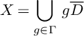

A fundamental domain D is locally finite if the set
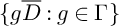 $\{g\overline {D}: g\in \Gamma \}$
is locally finite: that is, for each
 $x \in X$
, there is an
 $\epsilon> 0$
such that the open ball
 $B(x, \epsilon )$
of radius
 $\epsilon $
centered at x meets only finitely many members of
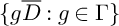 $\{g\overline {D}: g\in \Gamma \}$
.
Definition 3.22. Let
 $\Gamma $
be a group of homeomorphisms of a metric space X.
 $\Gamma $
is said to be discontinuous if for any compact subset K of X, the set
 $K\cap gK$
is empty except for only finitely many
 $g\in \Gamma $
.
Let
 $\Gamma $
be a discontinuous group of isometries of a hyperbolic n-space
 $H^{n}$
. By [Reference Ratcliffe17, Theorems 6.6.10 and 6.6.12], there is a point a such that the stabilizer group
 $\Gamma _{a}$
of a is trivial. For each
 $g\neq 1$
in
 $\Gamma $
, we set
 $H_{g}^{+}(a) = \{ x\in H^{n} : d_{H}(x, a) < d_{H}(x, ga) \}.$
Definition 3.23. The Dirichlet domain
 $D_{\Gamma }(a)$
for
 $\Gamma $
, with center a, is either
 $H^{n}$
if
 $\Gamma $
is trivial or
 $$\begin{align*}D_{\Gamma}(a)=\bigcap_{g\in \Gamma\backslash \{1\}}H_{g}^{+}(a).\end{align*}$$
Let
 $D_{\Gamma }(a)$
be the Dirichlet domain for
 $\Gamma $
with center a as above. By [Reference Ratcliffe17, Theorem 6.6.13],
 $D_{\Gamma }(a)$
is a locally finite fundamental domain for
 $\Gamma $
.
3.7 Limit sets
Definition 3.24. A point a of
 $\partial B^{n}$
is a limit point of a subgroup G of
 $M(B^{n})$
if there is a point
 $x\in B^{n}$
and a sequence
 $\{g_{i} \}$
of elements of
 $ G$
such that the sequence
 $\{g_{i}x\}_{i\in \mathbb {N}}$
converges to a. The set of limit points of G is called the limit set of G, and is denoted by
 $\Lambda (G)$
. The complement of
 $\Lambda (G)$
in
 $\partial B^{n}$
is called the ordinary set of G, and is denoted by
 $O(G).$
Definition 3.25. A point a of
 $\partial B^{n}$
is a bounded parabolic limit point of a discrete subgroup group
 $\Gamma $
of
 $M(B^{n})$
if a is a fixed point of a parabolic element of
 $\Gamma $
and the orbit space
 $ (\Lambda (\Gamma )\backslash \{a\})/\Gamma $
is compact.
Remark 3.26. The terms bounded parabolic limit point and cusped limit point are used to refer to the same notion in this article. Their equivalence is proved in [Reference Ratcliffe17]. For the definitions, see [Reference Ratcliffe17, p. 618], and for the equivalence, see [Reference Ratcliffe17, Theorem 12.6.4].
3.8 Geometrically finite discrete groups
Definition 3.27. Let
 $\Gamma $
be a discrete subgroup of
 $M(B^{n})$
with a parabolic element that fixes a point a of
 $\partial B^{n}$
. Let
 $\Gamma _{a}$
be the stabilizer group of a. A horoball
 $B(a)$
based at a is said to be a horocusped region for
 $\Gamma $
based at a if for each
 $g\in \Gamma \backslash \Gamma _{a}$
, we have
 $$\begin{align*}B(a) \cap gB(a) = \emptyset.\end{align*}$$
If a horocusped region
 $B(a)$
based at a is not maximal with respect to the inclusion relation,
 $B(a)$
is said to be proper.
Let
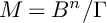 $M=B^n/\Gamma $
, and let
 $\pi : B^n \rightarrow M$
be the quotient map. Let
 $B(a)$
be a (proper) horocusped region based at a. The open subset
 $V=\pi (B(a))$
of M is called the (proper) horocusp of M corresponding to
 $B(a)$
.
Definition 3.28. Let
 $C(\Gamma )$
be the hyperbolic convex hull of the limit set
 $\Lambda (\Gamma )$
of
 $\Gamma $
. The convex core of
 $M=B^{n}/\Gamma $
is the set
 $$\begin{align*}C(M)= (C(\Gamma)\cap B^{n})/\Gamma.\end{align*}$$
Definition 3.29. Let
 $\Gamma $
be a discrete subgroup of
 $M(B^{n})$
, let
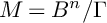 $M=B^{n}/\Gamma $
, and let
 $C(M)$
be the convex core of M. The group
 $\Gamma $
is said to be geometrically finite if there is a (possibly empty) finite union V of proper horocusps of M, with disjoint closures, such that
 $C(M)\backslash V$
is compact.
Theorem 3.30 [Reference Ratcliffe17, Theorem 12.4.10]
Let
 $\Gamma $
be a discrete subgroup of
 $M(B^{n})$
with an integer
 $n>1$
. Then, the following are equivalent:
-
(1) The orbit space
$B^{n}/\Gamma $
has finite volume. -
(2) The group
$\Gamma $
is geometrically finite and
$\Lambda (\Gamma )=\partial B^{n}$
. -
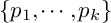
(3) There are finite points
$p_{1}, \cdots p_{k}$
of
$\overline {B^{n}}$
such that
$P\cap B^{n}$
is a fundamental domain with finite volume, where P is the hyperbolic convex hull of
$\{p_{1}, \cdots , p_{k}\}$
in
$\overline {B^{n}}.$






By [Reference Ratcliffe17, Theorems 12.6.4 and 12.6.5], we have the following theorem.
Theorem 3.31. Let
 $\Gamma $
be a discrete subgroup of
 $M(B^n)$
, and let C be the set of bounded parabolic limit points of
 $\Gamma $
. For each
 $c\in C$
, there exists a horocusped region
 $U(c)$
based at c for
 $\Gamma $
such that:
-
(1) the members of
$\{\overline {U}(c) : c\in C\}$
are mutually disjoint; -
(2)
$ \gamma U(c) = U(\gamma c)$
for any
$\gamma \in \Gamma $
and
$c \in C$
; -
(3)
$\{ \overline {U}(c)\backslash \{c\}\} $
is a locally finite family of closed subsets of
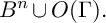
$B^{n}\cup O(\Gamma ).$



4 Cohomological dimension of groups
4.1 Cohomology of groups
In this section, we review some definitions and basic facts about cohomology of groups, which are contained in [Reference Brown8].
Definition 4.1. Let R be a ring and M be a left R-module. Let n be a non-negative integer. Then,
 $\operatorname {proj dim}_{R} M \leq n$
if there is a left projective resolution of length n:
 $$\begin{align*}0 \rightarrow P_{n} \rightarrow P_{n-1} \rightarrow \cdots \rightarrow P_{0} \rightarrow M \rightarrow 0.\end{align*}$$
The following lemma is well-known.
Lemma 4.2 [Reference Brown8, Chapter VIII, Lemma (2.1)]
The following conditions are equivalent:
-
(1)
$\operatorname {proj dim}_{R} M \leq n.$
-
(2)
$\operatorname {Ext}_{R}^{i} (M, -) = 0$
for all
$i>n$
. -
(3)
$\operatorname {Ext}_{R}^{n+1} (M, -) =0.$
-
(4) For any left R-module exact sequence
$0 \rightarrow K \rightarrow P_{n-1} \rightarrow \cdots \rightarrow P_{0}\rightarrow 0$
with
$P_{i}$
projective, K is projective.




Definition 4.3. We define the cohomological dimension
 $\operatorname {cd} \Gamma $
as following:
 $$ \begin{align*} \operatorname{cd} \Gamma &= \operatorname{projdim}_{\mathbb{Z} \Gamma} \mathbb{Z} \\ &= \inf\lbrace n : \mathbb{Z} {\text{ admits a projective resolution of length }}n \rbrace \\ &= \inf\lbrace n : H^{n}(\Gamma, -) = 0 {\text{ for all }} i>n \rbrace \\ &= {\sup}\lbrace n : H^{n}(\Gamma, M) \neq 0 {\text{ for some }} \Gamma{\text{-module }} M\rbrace. \end{align*} $$
Recall that the functor
 $\operatorname {Ext}_{R}^{i} (M, -)= H^{i} (\operatorname {Hom}_{R} (M,-))$
. Then,
 $\operatorname {Ext}_{\mathbb {Z}\Gamma }^{i} (\mathbb {Z}, -) = H^{i}(\Gamma , -)$
. By the previous Lemma, the above definition is well-defined.
The following theorem is called Serre’s theorem that claims well-definedness of the virtual cohomological dimension.
Theorem 4.4 [Reference Brown8, Chapter VIII, Theorem (3.1)]
If
 $\Gamma $
is a torsion-free group and
 $\Gamma ^{'}$
is a subgroup of finite index, then
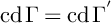 $\operatorname {cd} \Gamma = \operatorname {cd} \Gamma ^{'}$
.
Definition 4.5. Let
 $\Gamma $
be a virtually torsion-free group. By Theorem 4.4, any torsion-free subgroup of finite index has the same cohomological dimension. The dimension is called the virtual cohomological dimension, and is denoted by
 $\operatorname {vcd} \Gamma $
.
4.2 Bestvina–Mess formula
Definition 4.6. Let X be a topological space. The order of an open covering
 $\mathcal {U}$
of X is defined to be
 $$\begin{align*}\operatorname{ord}{\mathcal{U}} =\sup \{ k: {\text{there exist }} U_{1}, \dots, U_{k} \in \mathcal{U} {\text{ such that }} \cap_{i=1}^{k} U_{i} \neq \emptyset \} .\end{align*}$$
The covering dimension
 $\dim X$
of X is defined as follows:
 $\dim X \leq n$
if for any finite open covering
 $\mathcal {U}$
of X, there exists a finite open refinement
 $\mathcal {V}$
of
 $\mathcal {U}$
such that
 $\operatorname {ord}\mathcal {V} \leq n+1$
, and
 $\dim X=n$
if
 $\dim X \leq n$
and
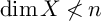 $\dim X \nless n$
.
Bestvina and Mess [Reference Bestvina and Mess5] proved the following formula for any virtually torsion-free hyperbolic group G:
 $$\begin{align*}\operatorname{vcd}G = \dim \partial G + 1,\end{align*}$$
where
 $\partial G$
is the Gromov boundary of G and
 $\dim \partial G$
is the covering dimension of
 $\partial G$
. In [Reference Bestvina6], this formula, called the Bestvina–Mess formula, is generalized for groups that admit
 $\mathcal {Z}$
-structures. Recently, Fukaya [Reference Fukaya10] proved the Bestvina–Mess formula for relatively hyperbolic groups.
Definition 4.7. A compact metrizable space X is a Euclidean retract (or ER) if X is finite-dimensional, contractible, and locally contractible.
Definition 4.8. Let X be an ER. A closed subset Z of X is called a
 $\mathcal {Z}$
-set if
 $X\backslash Z$
is homotopy dense in X, that is, there exists a homotopy
 $H:X\times \lbrack 0, 1\rbrack \rightarrow X$
such that
 $H_{0}= id$
, and
 $H_{t}(X) \subset X\backslash Z$
for any
 $t>0$
.
Definition 4.9. Let
 $\overline {X}$
be an ER, and let Z be a closed subset of
 $\overline {X}$
. A pair
 $(\overline {X}, Z)$
is a
 $\mathcal {Z}$
-structure for a group G if:
-
(1) Z is a
$\mathcal {Z}$
-set of
$\overline {X}$
. -
(2)
$\overline {X}\backslash Z$
admits a covering space action of G with compact quotient. -
(3) For any compact subset K of X and any open covering
$\mathcal {U}$
of
$\overline {X}$
, for all but finitely many
$g\in G$
, there exists
$U_{g} \in \mathcal {U}$
such that
$gK \subset U_{g}$
.


Theorem 4.10 [Reference Bestvina6, Theorem 1.7]
Let G be a virtually torsion-free group. If
 $(\overline {X}, Z)$
be a
 $\mathcal {Z}$
-structure on some torsion-free subgroup of G of finite index, then
 $\operatorname {vcd} G = \dim Z+1,$
where
 $\dim Z$
is the covering dimension of Z.
Example 4.11. Let
 $B^{n}$
be the n-dimensional conformal model of hyperbolic spaces. and let
 $\Gamma $
be a cocompact discrete subgroup of
 $M(B^n).$
Then, the pair
 $(\overline {B^{n}}, S^{n-1})$
is a
 $\mathcal {Z}$
-structure of a group
 $\Gamma $
, and so
 $\operatorname {vcd} \Gamma = \dim S^{n-1} +1 = n.$
5 Automorphism groups of K3 surfaces and virtual cohomological dimension
In this section, we consider the natural actions of the automorphism groups of K3 surfaces on hyperbolic spaces. First, we recall the constructions of hyperbolic spaces induced by hyperbolic lattices, and discuss the actions of the automorphism groups of K3 surfaces on certain hyperbolic spaces, and moreover, some properties of automorphism groups. Second, we discuss some invariants of automorphism groups, for example, the virtual cohomological dimension.
5.1 Geometrical finiteness of
$\operatorname {Aut}_{s}(X).$

Let X be an algebraic K3 surface with
 $\rho (X) \geq 3$
defined over
 $\mathbb {C}$
, and let f be the quadratic form defined by
 $f(x) = \langle x, x \rangle $
for
 $x \in NS(X) \otimes \mathbb {R}$
, where
 $\langle , \rangle $
is the inner product on
 $NS(X)$
induced by the cup product on
 $H^{2}(X, \mathbb {Z})$
. Since X is algebraic, f has the signature
 $(1, n)$
, where
 $n=\rho (X) -1.$
Then, there exists
 $M \in \mathrm {GL}(n+1, \mathbb {R})$
such that
 $f_{n+1}(Mx) = f(x)$
, where
 $f_{n+1}(x)=x_{0}^{2} -(x_{1}^{2}+x_{2}^{2}+ \cdots +x_{n}^{2}).$
Therefore, we can identify the connected component of the set
 $$\begin{align*}\{ x \in NS(X)\otimes \mathbb{R} : \langle x, x \rangle =1 \},\end{align*}$$
containing ample classes of X with the hyperboloid model of hyperbolic n-spaces. We denote this hyperboloid model of hyperbolic n-spaces by
 $\mathbb {H}^{n}_{X}$
. The hyperbolic distance function d on
 $\mathbb {H}^{n}_{X}$
satisfies
 $\cosh d(x, y) = \langle x, y \rangle .$
Remark 5.1. To construct the hyperboloid model of hyperbolic space, it is necessary that the Néron–Severi lattice
 $\mathrm {NS}(X)$
is of hyperbolic type as a lattice. Moreover, in order for the resulting hyperboloid model to have dimension at least two, its Picard rank must be at least three. Then, unless otherwise stated, we assume that X is algebraic and its Picard rank is at least three.
Definition 5.2. We call
 $\mathbb {H}^{n}_{X}$
the hyperbolic space associated with X. Let
 $\overline {P^{+}}(X)$
be the closure of the positive cone
 $P^{+}(X)$
in
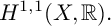 $H^{1,1}(X, \mathbb {R}).$
We define
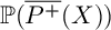 $\mathbb {P}(\overline {P^{+}}(X))$
by
 $$\begin{align*}\mathbb{P}(\overline{P^{+}}(X)) = (\overline{P^{+}}(X)\backslash \{0\})/\mathbb{R}_{> 0}.\end{align*}$$
For a point x in
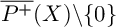 $\overline {P^{+}}(X)\backslash \{0\}$
, we denote by
 $\lbrack x \rbrack $
the class in
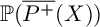 $\mathbb {P}(\overline {P^{+}}(X))$
corresponding to x. The inclusion from
 $\mathbb {H}^{n}_{X}$
to
 $\overline {P^{+}}(X)$
induces a continuous injective map
 $i :\mathbb {H}^{n}_{X}\rightarrow \mathbb {P}(\overline {P^{+}}(X)).$
Since i is a homeomorphism from
 $\mathbb {H}^{n}_{X}$
to
 $i(\mathbb {H}^{n}_{X})$
, we identify
 $\mathbb {H}^{n}_{X}$
with
 $i(\mathbb {H}^{n}_{X}).$
The boundary of
 $\mathbb {H}^{n}_{X}$
at infinity, denoted by
 $\partial {\mathbb {H}}^{n}_{X}$
, is the boundary of
 $i(\mathbb {H}^{n}_{X})$
in
 $\mathbb {P}(\overline {P^{+}}(X)),$
which is equal to the set
 $\{ x \in (\mathrm {NS}(X)\otimes \mathbb {R}) \cap \overline {P^{+}}(X)\backslash \{0\}: \langle x, x \rangle =0\}/\mathbb {R}_{> 0}.$
We set
 $\overline {\mathbb {H}}^{n}_{X} = \mathbb {H}^{n}_{X} \cup \partial {\mathbb {H}}^{n}_{X}.$
Definition 5.3. Let
 $A(X)$
be the ample cone of X. We define

The closure of
 $A_{X}$
in
 $\overline {\mathbb {H}^{n}_{X}}$
is denoted by
 $\overline {A_{X}}.$
We denote
 $\overline {A_{X}}\backslash A_{X}$
by
 $\partial A_{X}$
, called the boundary associated with the ample cone of X.
By the unimodulality of
 $H^{2}(X, \mathbb {Z})$
, the discriminant groups of
 $NS(X)$
and
 $T_{X}$
are isomorphic:
 $$\begin{align*}A_{NS(X)} = NS(X)^{*}/NS(X) \simeq T_{X}^{*}/T_{X} = A_{T_{X}}.\end{align*}$$
Each isomorphism
 $\phi $
of
 $NS(X)$
or
 $T_{X}$
gives rise to an isomorphism of the group
 ${A_{NS(X)} \simeq A_{T_{X}}}$
, denoted by
 $\phi ^{*}$
. Since the automorphism group
 $\operatorname {Aut}(X)$
of X naturally acts on the ample cone of X, there is a natural homomorphism
 $\rho : \operatorname {Aut} (X) \rightarrow \operatorname {Aut}(A(X)).$
As for this homomorphism, the following theorem is well-known.
Theorem 5.4 [Reference Kondo14, Theorem 8.1]
The kernel and the cokernel of
 $\rho $
are finite groups.
Since
 $\operatorname {Aut}(X)$
is finitely generated [Reference Sterk19, Proposition 2.2] and Selberg’s Lemma [Reference Alperlin1],
 $\operatorname {Aut}(X)$
is virtually torsion-free.
Definition 5.5. Let X be a K3 surface, and let
 $\omega _{X}$
be a nowhere vanishing holomorphic 2-form of X. An automorphism
 $\phi $
of X is said to be symplectic if
 $\phi $
acts trivially on
 $\omega _{x}$
. The symplectic automorphism group of X, denoted by
 $\operatorname {Aut}_{s}(X)$
, is the group of symplectic automorphisms of X.
The following lemma is well-known.
Lemma 5.6 [Reference Kondo14, Lemma 8.11]
The symplectic automorphism of X acts trivially on the transcendental lattice
 $T_{X}$
.
Let
 $\phi $
be the symplectic automorphism of X. Then, by Lemma 5.6,
 $\phi $
acts trivially on
 $A_{NS(X)}\simeq A_{T_{X}}.$
By the Torelli Theorem [Reference Burns and Rapoport7] and [Reference Piatetski-Shapiro and Shafarevich16], we can identify
 $\operatorname {Aut}_{s}(X)$
with the subgroup
 $\{ \phi \in O^{+}(NS(X)) : \phi A(X) = A(X) , \phi ^{*}|_{A_{NS(X)}} = \mathrm {id}_{A_{NS(X)}} \}$
. Therefore,
 $\operatorname {Aut}_{s}(X)$
is a subgroup of finite index in
 $\operatorname {Aut}(A(X)).$
Since any element of
 $O^{+}(NS(X))$
is an isometry of the hyperbolic space
 $\mathbb {H}^{n}_{X}$
associated with X, the symplectic automorphism group
 $\operatorname {Aut}_{s}(X)$
of X is a discrete subgroup of isometries of
 $\mathbb {H}^{n}_{X}$
.
Proposition 5.7. Let X be an algebraic K3 surface with
 $\rho (X) \geq 3$
, and let
 $a \in A_{X}.$
Then, the Dirichlet domain
 $D(a)$
of
 $\mathbb {H}^{n}_{X}$
, with center a, for the reflection group
 $W(X)$
is equal to
 $A_{X}=A(X)\cap \mathbb {H}^{n}_{X}.$
Proof. Recall that
 $H^{+}_{w}(a) = \{ x \in \mathbb {H}_{X}^{n} : d(x, a) < d(x, wa) \hspace {1mm}\}$
for
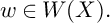 $w \in W(X).$
If w is the reflection
 $s_{\delta }$
for some root
 $\delta $
,
 $$ \begin{align*} &\hspace{7mm} d(x, a)< d(x, s_{\delta}a) \\ &\Leftrightarrow \hspace{1mm} \cosh d(x, a) < \cosh d(x, s_{\delta}a) \\ &\Leftrightarrow \hspace{1mm} \langle x, a \rangle < \langle x, s_{\delta}a \rangle \\ &\Leftrightarrow \hspace{2mm} 0< \langle a, \delta \rangle \langle x, \delta \rangle \\ &\Leftrightarrow \hspace{2mm} 0< \langle x, \delta \rangle. \end{align*} $$
Then, we have that
 $H^{+}_{s_{\delta }}(a) = \{x \in \mathbb {H}^{n}_{X}: \langle x, \delta \rangle>0 \}.$
Since
 $A_{X}$
is a fundamental domain for
 $W(X)$
on
 $\mathbb {H}^{n}_{X}$
whose sides are bounded by roots of
 $\operatorname {NS}(X)$
, we have
 $A_{X}=\cap _{\delta \in \Delta ^{+}(X)} H^{+}_{s_{\delta }}.$
By the definition of
 $D(a)$
, we have
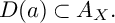 $D(a) \subset A_{X}.$
Since
 $D(a)$
and
 $A_{X}$
are convex fundamental domains for
 $W(X)$
, we have
 $D(a)=A_{X}.$
By [Reference Ratcliffe17, Theorem 12.8.4], the orbit space
 $\mathbb {H}^n_{X}/O^{+}(\mathrm {NS}(X))$
has finite volume. By Theorem 3.30, we have the following.
Lemma 5.8. Let X be an algebraic K3 surface with
 $\rho (X) \geq 3$
. Then,
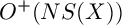 $O^{+}(NS(X))$
is geometrically finite and of the first kind (i.e., its limit set is equal to
 $S^{n-1}$
). Moreover, a fundamental domain of
 $\mathbb {H}^{n}_{X}$
for
 $O^{+}(NS(X))$
is a generalized polytope; that is, the fundamental domain is the convex hull of finitely many vertices, which may lie on the boundary at infinity.
Lemma 5.9. Let
 $a \in A_{X}$
, and let P be the Dirichlet domain, centered at a, of
 $\mathbb {H}^{n}_{X}$
for
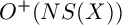 $O^{+}(NS(X))$
. Then,
 $\operatorname {Aut}(A(X))\cdot \overline {P} = \overline {A_{X}}^{H}$
, where
 $\overline {P}$
(resp.
 $\overline {A_{X}}^{H}$
) are the closure of P (resp.
 $A_{X}$
) in
 $\mathbb {H}^{n}_{X}.$
Proof. By Lemma 5.7 and the definition of P, we have
 $$ \begin{align*} P &=\{ x\in \mathbb{H}^{n}_{X}: d(x,a) <d(x, ga) {\text{ for any }} g \neq 1 {\text{ in }} O^{+}(NS(X)) \}, \\ A_{X} &= \{ x\in \mathbb{H}^{n}_{X}: d(x,a) <d(x, wa) {\text{ for any }} w \neq 1 {\text{ in }} W(X) \}. \end{align*} $$
Then, we have
 $P \subset A_{X}$
and so
 $\overline {P} \subset \overline {A_{X}}^{H}.$
Hence, we obtain
 $\operatorname {Aut}(A(X))\cdot \overline {P} \subset \overline {A_{X}}^{H}.$
Conversely, because the tessellation
 $\{g\overline {P}: g\in O^{+}(NS(X))\}$
of
 $\mathbb {H}^{n}_{X}$
is locally finite, the union
 $\operatorname {Aut}(A(X))\cdot \overline {P}$
is a closed subset. Then, it is enough to show that
 $A_{X}\subset \operatorname {Aut}(A(X))\cdot \overline {P}.$
For any
 $x\in A_{X}$
, there exist
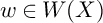 $w \in W(X)$
and
 $\gamma \in \operatorname {Aut}(A(X))$
such that
 $x \in w\gamma \overline {P}.$
Then, we have
 $x \in w\gamma \overline {P}\cap A_{X} \subset w\overline {A_{X}}^{H}\cap A_{X}.$
By [Reference Ratcliffe17, Theorem 6.6.4], we have
 $w=1$
. In particular, we have
 $x\in \gamma \overline {P}$
. Hence, we have
 $A_{X}\subset \operatorname {Aut}(A(X))\cdot \overline {P}$
.
Definition 5.10. Let P be the same as in Lemma 5.9. We define sets of bounded parabolic limit points of
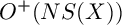 $O^{+}(NS(X))$
as follows:
-
•
$I_{P} =$
the set of ideal vertices of P; -
•
$V = Aut(A(X))\cdot I_{P}$
; -
•
$V_{NS}= O^{+}(NS(X))\cdot I_{P};$
-
•
$V_{X} = \{c \in V : \operatorname {vcd} W(X)_{c} < n-1 \},$




where
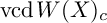 $\operatorname {vcd} W(X)_{c}$
is the stabilizer group of
 $W(X)$
at a point c.
Definition 5.11. Let X be an algebraic K3 surface with
 $\rho (X)\geq 3$
. Since
 $\operatorname {Aut}_{s}(X)$
is of finite index in
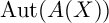 $\operatorname {Aut}(A(X))$
, the limit set of
 $\operatorname {Aut}_{s}(X)$
is equal to that of
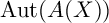 $\operatorname {Aut}(A(X))$
. We denote this limit set by
 $\Lambda _{X}$
, and is called the limit set of the K3 surface X. We denote the hyperbolic convex hull of
 $\Lambda _{X}$
by
 $C(X)$
, and put
 $B(X) = C(X) \cap \mathbb {H}^{n}_{X}$
.
Lemma 5.12. For any
 $c\in V\backslash V_{X}$
, there exists a horoball
 $U(c)$
based at c such that
 $B(X)\cap U(c) =\varnothing $
. Moreover, the point c is isolated in the boundary
 $\partial A_{X}$
associated with the ample cone.
Proof. If
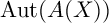 $\operatorname {Aut}(A(X))$
is elementary, this lemma is obvious.
Suppose that
 $\operatorname {Aut}(A(X))$
is non-elementary. Let
 $\phi :\mathbb {H}^{n}_{X} \rightarrow U^{n}$
be an isometry from
 $\mathbb {H}^{n}_{X}$
to the upper half-space model
 $U^{n}$
such that
 $\phi (c) = \infty .$
The isometry
 $\phi $
induces the natural homeomorphisms from
 $\partial \mathbb {H}^{n}_{X}\backslash \{ c\}$
to
 $\partial U^{n}.$
We also denote this homeomorphism by
 $\phi $
. Let b be a point of
 $U^{n}$
corresponding to a point a in
 $A_{X}$
. We can consider the stabilizer group
 $W(X)_{\infty }$
as the Poincaré extension of a subgroup of
 $I(E^{n-1})$
. Since
 $\operatorname {vcd} W(X)_{c} = n-1$
,
 $W(X)_{\infty }$
is a crystallographic group of
 $E^{n-1}$
. Then, the Dirichlet domain K of
 $E^{n-1}$
for
 $W(X)_{\infty }$
, centered at b, is compact. Proposition 5.9 implies that
 $\Lambda _{X} \subset \partial A_{X}.$
Then, we have
 $\phi (\Lambda _{X}) \subset K\cup \{\infty \}.$
Since
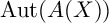 $\operatorname {Aut}(A(X))$
is non-elementary, the limit set
 $\Lambda _{X}$
is perfect: that is, every point of
 $\Lambda _{X}$
is not isolated. Hence, the infinity
 $\infty $
is not in
 $\phi (\Lambda _{X})$
. By the compactaness of K, there exists a horoball
 $B_{\infty }$
based at
 $\infty $
such that
 $C(K)\cap B_{\infty } = \varnothing ,$
where
 $C(K)$
is the hyperbolic convex hull of K. In particular,
 $B(X) \cap B_{\infty }=\varnothing .$
The inverse image
 $\phi ^{-1}(B_{\infty })$
of
 $B_{\infty }$
by
 $\phi $
is the desired horoball.
Lemma 5.13. Let e be an elliptic divisor of X, let
 $f_{e}$
be an elliptic fibration associated to e, and let
 $\operatorname {Aut}(X)_{e}$
be the stabilizer group of e. Then,
 $$\begin{align*}\operatorname{vcd{\operatorname{Aut}(X)_{e}}} = \operatorname{vcd} \operatorname{MW}(f_{e}) {\text{, and }} \operatorname{vcd}W(X)_{e} = \sum_{v\in \mathbb{P}^{1}}{(m_{v}-1)},\end{align*}$$
where
 $\mathrm {MW}(f_{e})$
is the Mordell-Weil group of
 $f_{e}$
, and
 $m_{v}$
be the number of connected components of the fiber
 $f^{-1}(v)$
for
 $v\in \mathbb {P}^{1}.$
Proof. Let v be a point in
 $\mathbb {P}^{1},$
and let
 $m_{v}$
be the number of connected components of the fiber
 $f^{-1}(v)$
. By Shioda–Tate formula,
 $$\begin{align*}\rho(X)-2 = \operatorname{vcd}{MW(f_{e})} + \sum_{v\in \mathbb{P}^{1}}{(m_{v}-1)}.\end{align*}$$
If
 $m_{v}\neq 1$
, we denote by
 $W_{v}$
the Weyl group generated by the connected components of
 $f^{-1}(v)$
, which is of type
 $\tilde {A}$
,
 $\tilde {D}$
, or
 $\tilde {E}.$
Since
 $W_{v}$
fixes the elliptic divisor e, we have
 $\oplus W_{v} \subset W(X)_{e}.$
Here, for each v with
 $m_{v}\neq 1$
, the Weyl group
 $W_{v}$
acts on the
 $(m_{v}-1)$
-dimensional Euclidean space, and admits an
 $(m_{v}-1)$
-dimensional simplex
 $\Delta _{v}$
as a fundamental domain for the action of
 $W_{v}.$
Hence,
 $\oplus W_{v}$
acts on the
 $(\sum _{v\in \mathbb {P}^{1}}{(m_{v}-1})\big )$
-dimensional Euclidean space, and has the fundamental domain
 $\prod _{v}{\Delta _{v}}$
. Then, we have
 $$\begin{align*}\sum_{v \in \mathbb{P}^{1}}(m_{v}-1) = \operatorname{vcd}(\oplus W_{v}) \leq \operatorname{vcd}W(X)_{e}.\end{align*}$$
Since the Mordell–Weil group of
 $f_{e}$
is a subgroup of
 $\operatorname {Aut}(X)_{e}$
, then
 $\operatorname {rk} \operatorname {MW}f_{e} \leq \operatorname {vcd}\operatorname {Aut}(X)_{e}$
, where
 $\operatorname {rk} \operatorname {MW} f_{e}$
is the rank of Mordell–Weil group of
 $f_{e}$
.
Since both
 $W(X)_{e}$
and
 $\operatorname {Aut}(X)_{e}$
fix the elliptic divisor e, which is a cusped limit points of
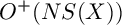 $O^{+}(NS(X))$
, these two groups are elementary of either elliptic or parabolic type. Therefore, there exists an integer l (resp. m) such that
 $W(X)_{e}$
(resp.
 $\operatorname {Aut}(X)_{e}$
) has a subgroup that is isomorphic to
 $\mathbb {Z}^{l}$
(resp.
 $\mathbb {Z}^{m}$
) of finite index in
 $W(X)_{e}$
(resp.
 $\operatorname {Aut}(X)_{e}$
). Hence, we have
 $$ \begin{align} \sum_{v\in \mathbb{P}^{1}}{(m_{v}-1)} \leq l , \end{align} $$
 $$ \begin{align} \operatorname{rk} \operatorname{MW} f_{e} \leq m , \end{align} $$
so that
 $\rho (X)-2 \leq l+m.$
On the other hand,
 $O^{+}(NS(X))_{e}$
has a subgroup that is isomorphic to
 $\mathbb {Z}^{l+m}.$
Then,
 $l+m = \rho (X)-2.$
Inequalities (5.1) and (5.2) imply that
 $$ \begin{align*} l = \sum_{v \in \mathbb{P}^{1}}(m_{v}-1), \\ m = \operatorname{rk} \operatorname{MW} f_{e}. \end{align*} $$
These are namely the desired equalities.
By Lemma 5.13, we have
 $V_{X} = \{c \in V : \operatorname {vcd}\operatorname {Aut}(X)_{c} \geq 1 \} = \{c \in V : \operatorname {vcd}\operatorname {Aut}(A(X))_{c} \geq 1 \}.$
Then, each element of
 $V_{X}$
is fixed by some parabolic transformation of
 $\operatorname {Aut}(A(X))_{c}.$
As noted in the introduction, the following theorem is also found by Kohei Kikuta at about the same time (see the introduction for details).
Theorem 5.14. Let X be an algebraic K3 surface with
 $\rho (X)\geq 3$
, and let
 $\operatorname {Aut}_{s}(X)$
be the symplectic automorphism group of X. Then,
 $\operatorname {Aut}_{s}(X)$
is geometrically finite.
Proof. By Theorem 5.4, the symplectic automorphism group
 $\operatorname {Aut}_{s}(X)$
is a subgroup of finite index in
 $\operatorname {Aut}(A(X)).$
Then, it is enough to show that
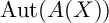 $\operatorname {Aut}(A(X))$
is geometrically finite. Recall the notation of P, V,
 $V_{NS}$
, and
 $V_{X}$
in Definition 5.10
By Theorem 3.31, there exist proper horoballs at
 $c \in V_{NS}$
such that:
-
(1)
$\{ \overline {U(c)} : c \in V_{NS}\}$
are mutually disjoint; -
(2)
$gU(c) = U(gc)$
for any element
$g \in O^{+}(NS(X))$
; -
(3)
$\{\overline {U(c)}\backslash {c} \} $
is locally finite in
$\mathbb {H}^{n}_{X}$
.





By Lemma 5.12, shrinking the horoballs
 $U(c)$
sufficiently small, we obtain that
 $$\begin{align*}B(X)\backslash \bigcup_{c\in V_{X}} U(c) = B(X)\backslash \bigcup_{c\in V} U(c).\end{align*}$$
By applying Lemma 5.9,
 $$ \begin{align*} B(X)\backslash \bigcup_{c\in V_{X}} U(c) &\subset \hspace{1mm}\overline{A_{X}}^{H}\backslash \bigcup_{c\in V} U(c) \\ &= \big( \bigcup_{g\in \operatorname{Aut}(A(X))}\hspace{-1mm}g\overline{P}\hspace{1mm}\big) \big\backslash \bigcup_{c\in V} U(c) \\ &= \bigcup_{g\in \operatorname{Aut} (A(X))} \big(g\overline{P} \hspace{1mm} \backslash \bigcup_{c\in V} U(c) \big)\\ &= \bigcup_{g \in \operatorname{Aut}(A(X))}g(\overline{P}\backslash \bigcup_{c \in V} U(c)). \end{align*} $$
Hence, we have
 $$ \begin{align} B(X)\backslash \bigcup_{c\in V_{X}} U(c) \subset \bigcup_{g \in \operatorname{Aut}(A(X))}g(\overline{P}\backslash \bigcup_{c \in V} U(c)). \end{align} $$
Let
 $\pi :\mathbb {H}^{n}_{X} \rightarrow \mathbb {H}^{n}_{X}/\hspace {-1mm}\operatorname {Aut}(A(X))$
be the natural quotient map. We define
 $V_{c} = U(c)/\operatorname {Aut}(A(X)).$
By the inclusion 5.3, we obtain
 $$\begin{align*}(B(X)/\operatorname{Aut}(A(X)))\backslash \bigcup_{c\in I_{P}\cap V_{X}}V_{c} \subset \pi(\overline{P}\backslash \bigcup_{c\in V} U(c)).\end{align*}$$
By Lemma 5.8, P is a generalized polytope. For each vertex c of P in the boundary at infinity, we have the corresponding horoball
 $U(c)$
. Therefore, the set
 $\overline {P}\backslash \bigcup _{c \in V} U(c))$
is obtained by removing the parts at infinity from
 $\overline {P}$
, and is compact. Then,
 $(B(X)/\operatorname {Aut}(A(X)))\backslash \bigcup _{c\in I_{P}\cap V_{X}}V_{c}$
is compact and
 $\{ V_{c}\}_{c\in I_{P}\cap V_{X}}$
is a set of finitely many horocusps with disjoint closures. By Definition 3.29,
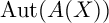 $\operatorname {Aut}(A(X))$
is geometrically finite.
Proposition 5.15. Let p be a cusped limit point of
 $\operatorname {Aut}(A(X)).$
Then, p is a horopoint of
 $\overline {A_{X}},$
that is, there exists a horoball U based at p such that U meets just the sides of
 $\overline {A_{X}}$
incident with p.
Proof. We now pass to the upper half-space model
 $U^n$
and conjugate
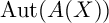 $\operatorname {Aut}(A(X))$
so that
 $p=\infty .$
Let P be a Dirichlet polyhedron P, centered at
 $a\in A_{X}$
, for
 $O^{+}(NS(X)).$
From the proof of [Reference Ratcliffe17, Theorem 12.4.4], there exist a horoball
 $\Sigma $
based at
 $\infty $
and elements
 $g_{1}, \ldots , g_{k}$
in
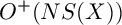 $O^{+}(NS(X))$
such that
 $$\begin{align*}\Sigma \subset \bigcup_{f\in O^{+}(\mathrm{NS}(X))_{\infty}}f ( \bigcup_{i=1}^{k}g_{i}\overline{P}) \end{align*}$$
and
 $\Sigma $
meets just the vertical sides of
 $fg_{i}P$
.
Let S be a side of
 $A_{X}$
with
 $S \cap \Sigma \neq \varnothing .$
There exists an element
 $x\in S$
and
 $r>0$
such that
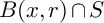 $B(x, r)\cap S $
is homeomorphic to
 $B^{n-1}.$
Since P is locally finite, shrinking r, there exists
 $h_{1}, {\ldots }, h_{l} \in O^{+}(NS(X))$
such that
 $x\in h_{j}\overline {P}$
and
 $B(x, r) \subset \bigcup _{j=1}^{l}h_{j}\overline {P}.$
In particular, we have
 $$ \begin{align*}B^{n-1} \cong B(x, r)\cap S \subset \bigcup \big\{ h_{j}T: h_{j}\in O^{+}(\mathrm{NS}(X)), T {\text{ is a side of }} \overline{P}, {\text{and }} x\in h_{j}T \big\}.\end{align*} $$
Hence, there exists a side T of
 $g\overline {P}$
such that
 $T^{\circ } \cap S\neq \varnothing .$
By [Reference Ratcliffe17, Theorem 6.3.8], we have
 $T\subset S.$
By
 $x\in T\cap \Sigma $
, then T is a vertical side of
 $g\overline {P}.$
Therefore, we have
 $\infty \in T \subset S$
.
There is a natural one-to-one correspondence between the set of maximal parabolic subgroups of
 $\operatorname {Aut}_{s}(X)$
and the set of rational rays in
 $\partial A(X)$
whose stabilizer subgroup in
 $\operatorname {Aut}_{s}(X)$
has rank at least one. By multiplying a positive integer, we have a primitive element in
 $NS(X)$
. From this argument and Lemma 5.13, we have the following proposition.
Proposition 5.16. Let P be a maximal parabolic subgroup of
 $\operatorname {Aut}_{s}(X).$
Then, there exists an element
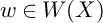 $w \in W(X)$
such that the fixed point of
 $wPw^{-1}$
is an elliptic divisor e. Moreover, the rank of P is equal to the rank of the Mordell-Weil group of the elliptic fibration
 $f_{e}$
associated with e.
5.2 The blown-up boundary of ample cones of K3 surfaces
The notion of the blown-up coronae for relatively hyperbolic groups (a generalization of geometrically finite groups) is defined in the paper of Fukaya–Oguni [Reference Fukaya and Oguni11], and Fukaya [Reference Fukaya10] established Bestvina–Mess type formula for relatively hyperbolic groups. We can immediately obtain Theorem 1 by applying Fukaya’s result [Reference Fukaya10, Corollary B].
For readability to algebraic geometers, in this section, we give a simplified version of Fukaya’s result, using the geometry of ample cones of K3 surfaces and hyperbolic geometry. Note that the proof method and some definitions in this section are not itself new.
Definition 5.17. Let U be an open subset of
 $\mathbb {R}^{n}$
, and let p be a point in U. We denote the
 $(n-1)$
-dimensional unit sphere in
 $\mathbb {R}^{n}$
by
 $S^{n-1}$
. We put
 $$\begin{align*}\operatorname{Bl}_{p}(U) = \{ (x, t) \in U\times S^{n-1}: |x-p|t = (x-p) \},\end{align*}$$
where
 $| \cdot |$
is the Euclidean norm. We define a function
 $\pi _{p}: \operatorname {Bl}_{p}(U) \rightarrow U$
by setting
 $\pi _{p}(x, t) = x.$
We call the function
 $\pi _{p}$
the blowing-up of U at a point p (to
 $S^{n-1}$
). For a subset A of U, the closure of
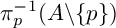 $\pi _{p}^{-1}(A\backslash \{p\})$
in
 $\operatorname {Bl}_{p}(U)$
is called the strict transform of A at a point p, and is denoted by
 $\operatorname {St}_{p}(A)$
.
Since
 $\pi _{p}$
restricts to a homeomorphism from
 $\mathrm {Bl}_{p}(U)\backslash \pi ^{-1}_{p}(p)$
to
 $U\backslash \{p\},$
we identify these two spaces.
Definition 5.18. Let
 $\mathcal {P}=\{p_{1}, \dots , p_{m}\}$
be a subset of U. For each
 $p\in \mathcal {P}$
, we take an open neighborhood
 $U_{p}$
of p such that
 $U_{p} \cap \mathcal {P} = \{p\}.$
Let
 $\pi _{p_{i}}: \operatorname {Bl}_{p_{i}}(U_{p_{i}}) \rightarrow U_{p_{i}}$
be the blowing-up of
 $U_{p_{i}}$
at a point
 $p_{i}$
. We define
 $\mathrm {Bl}_{\mathcal {P}}(U)$
by
 $$\begin{align*}\mathrm{Bl}_{\mathcal{P}}(U) = (U\backslash \mathcal{P}) \amalg ({\coprod_{p\in \mathcal{P}} \mathrm{Bl}_{p}(U_{p})})/\sim,\end{align*}$$
where the equivalence relation
 $\sim $
is generated by
 $x\sim \pi _{p_{i}}(x,t)$
for all
 $(x, t) \in \coprod _{p \in \mathcal {P}} \pi _{p}^{-1}(U_{p}\backslash \lbrace p\rbrace ).$
We denote by
 $\lbrack x \rbrack $
(resp.
 $\lbrack x, t\rbrack $
) the class in
 $\mathrm {Bl}_{\mathcal {P}}(U)$
corresponding to x (resp.
 $(x,t)$
). We define the function
 $\pi _{\mathcal {P}}: \operatorname {Bl}_{\mathcal {P}}(U) \rightarrow U$
by setting
 $$\begin{align*}\left\{ \begin{array}{@{}ll} \pi_{\mathcal{P}}(\lbrack x \rbrack) = x & (x \in U\backslash \mathcal{P}), \\ \pi_{\mathcal{P}}(\lbrack x, t \rbrack) = x & ( (x,t) \in \operatorname{Bl}_{p}(U_{p}), p\in \mathcal{P}). \end{array} \right.\end{align*}$$
We call the function
 $\pi _{\mathcal {P}}$
the blowing-up of U at a subset
 $\mathcal {P}$
. For a subset A of U, the closure of
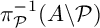 $\pi _{\mathcal {P}}^{-1}(A\backslash \mathcal {P})$
in
 $\operatorname {Bl}_{\mathcal {P}}(U)$
is called the strict transform of A at a subset
 $\mathcal {P}$
, and is denoted by
 $\operatorname {St}_{\mathcal {P}}(A)$
.
Definition 5.19. Let
 $\Gamma $
be a geometrically finite subgroup of
 $M(B^{n})$
, and let C be the set of cusped limit points of
 $\Gamma $
. For finite subsets
 $\mathcal {P}$
and
 $\mathcal {Q}$
of C with
 $\mathcal {P}\subset \mathcal {Q}$
, there exists the natural projection
 $\pi _{\mathcal {P}, \mathcal {Q}}: \operatorname {Bl}_{\mathcal {Q}}(\mathbb {R}^{n})\rightarrow \operatorname {Bl}_{\mathcal {P}}(\mathbb {R}^{n})$
such that
 $\pi _{\mathcal {P}}\circ \pi _{\mathcal {P}, \mathcal {Q}} = \pi _{\mathcal {Q}}.$
We denote the projective limit of (
 $\operatorname {Bl}_{\mathcal {P}}(\mathbb {R}^{n})$
,
 $\pi _{\mathcal {P}, \mathcal {Q}}$
) by
 $\pi _{C} = \varprojlim \pi _{\mathcal {P}} : \operatorname {Bl}_{C}(\mathbb {R}^{n})\rightarrow \mathbb {R}^{n}.$
We call the function
 $\pi _{C}$
the blowing-up of
 $\mathbb {R}^{n}$
at C. For a subset A of
 $\mathbb {R}^{n}$
, the closure of
 $\pi _{C}^{-1}(A\backslash \mathcal {P})$
in
 $\operatorname {Bl}_{C}(\mathbb {R}^n)$
is called the strict transform of A at C, and is denoted by
 $\operatorname {St}_{C}(A)$
. The strict transform of
 $\overline {B^{n}}$
(resp.
 $\partial B^{n}$
) is denoted by
 $\overline {B}^{bl}$
(resp.
 $\partial B^{bl}$
).
Lemma 5.20. The action of a geometrically finite subgroup
 $\Gamma $
of
 $M(B^{n})$
on
 $\mathbb {R}^{n}$
(resp.
 $B^{n}$
,
 $\partial B^{n}$
) is extended to a natural action on
 $\operatorname {Bl}_{C}(\mathbb {R}^{n})$
(resp.
 $\overline {B}^{bl}$
,
 $\partial B^{bl}$
).
Proof. Since
 $\Gamma $
preserves the cusped limit point of
 $\Gamma $
, the action of
 $\Gamma $
on
 $\mathbb {R}^{n}$
can be extend to that on
 $\operatorname {Bl}_{C}(\mathbb {R}^{n}).$
As
 $\Gamma $
preserves
 $\overline {B^{n}}$
and
 $\partial B^n$
,
 $\Gamma $
acts on
 $\overline {B}^{bl}$
(resp.
 $\partial B^{bl}$
).
Definition 5.21. Let
 $\Gamma $
be a geometrically finite subgroup of
 $M(B^{n})$
. A point a of
 $\partial B^{bl}$
is a limit point of
 $\Gamma $
in
 $\partial B^{bl}$
if there is a point
 $x\in B^{n}$
and there exists a sequence
 $\{g_{i}\}_{i\in \mathbb {N}}$
of
 $\Gamma $
such that
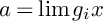 $a= \lim g_{i}x$
. The set of limit points of
 $\Gamma $
in
 $\partial B^{bl}$
is called the blown-up limit set of
 $\Gamma $
, and is denoted by
 $\Lambda ^{bl}(\Gamma ).$
Lemma 5.22. Let
 $\eta : U^{n} \rightarrow B^{n}$
be the standard transformation from
 $U^{n}$
to
 $B^{n}$
. For non-zero vector
 $v\in \partial U = E^{n-1}$
and
 $a\in \overline {U^{n}}$
, we define a half line
 $l:\lbrack 0, \infty ) \rightarrow \overline {U^{n}} $
by
 $l(t) = tv+a$
, and put
 $L(t)= (\eta \circ l)(t).$
Then,
 $$\begin{align*}\operatorname{St}_{e_{n}}(\operatorname{Im}(L)) \cap \pi^{-1}_{e_{n}}(e_{n})= \Big\{(e_{n}, \frac{v}{|v|})\Big\} \subset \operatorname{Bl}_{e_{n}}(\mathbb{R}^{n}). \end{align*}$$
In particular, the intersection of
 $\operatorname {St}_{e_{n}}(\operatorname {Im}(L))$
with
 $\pi ^{-1}_{e_{n}}(e_{n})$
is determined by the direction of v.
Proof. By direct calculation, we obtain
 $$\begin{align*}L(t)- e_{n} = \frac{2(tv+\rho(a)-e_{n})}{|tv+\rho(a)-e_{n}|^{2}}.\end{align*}$$
Then,
 $$\begin{align*}\lim_{t\rightarrow \infty} \frac{L(t)- e_{n}}{|L(t)- e_{n}|} =\lim_{t\rightarrow \infty}\frac{tv+\rho(a)-e_{n}}{|tv+\rho(a)-e_{n}|} = \frac{v}{|v|}.\end{align*}$$
Hence,
 $\displaystyle \operatorname {St}_{e_{n}}(\mathrm {Im}(L)) = \mathrm {Im}(L) \cup \{ (e_{n}, \frac {v}{|v|})\}.$
Corollary 5.23. Let V be a vector subspace of
 $\partial U^n= E^{n-1}$
, and let a be a point of
 $\overline {U^{n}}$
. Let A be an open
 $\epsilon $
-neighborhood of
 $V+a$
in
 $U^n$
for a positive number
 $\epsilon $
. Then,
 $$\begin{align*}\operatorname{St}_{e_{n}}(\eta(A)) \cap \pi^{-1}_{e_{n}}(e_{n}) = \Big\{ (e_{n}, \frac{v}{|v|}) \in \operatorname{Bl}_{e_{n}}(\mathbb{R}^{n}) : v\in V\backslash \{0\} \Big\} \cong S^{r-1}, \end{align*}$$
where r is the dimension of the vector space V.
Lemma 5.24. Let
 $\Gamma $
be a geometrically finite subgroup of
 $M(B^{n})$
. For every cusped limit point p of
 $\Gamma $
, we have
 $$\begin{align*}\Lambda^{bl}(\Gamma) \cap \pi_{C}^{-1}(p) =\Lambda^{bl}(\Gamma_{p}) \cong S^{r-1},\end{align*}$$
where r is the rank of the stabilizer group
 $\Gamma _{p}$
, that is, the rank of maximal abelian subgroup of
 $\Gamma _{p}$
.
Proof. By conjugating
 $\Gamma $
in
 $M(B^{n})$
, we can suppose
 $p=e_{n}.$
Let
 $\eta : U^{n} \rightarrow B^{n}$
be the standard transformation. The group
 $\Gamma $
acts on
 $U^n$
by setting
 $\gamma (x) = (\eta ^{-1}\gamma \eta ) (x) $
for any
 $\gamma \in \Gamma .$
Here, the point
 $p=e_{n}$
corresponds to the point
 $\infty $
at infinity of
 $U^n$
under the standard transformation
 $\eta $
.
First, we show that
 $\Lambda ^{bl}(\Gamma _{p}) \cong S^{r-1}.$
There is a
 $\Gamma _{\infty }$
-invariant r-plane Q of
 $E^{n-1}$
such that
 $Q/\Gamma _{\infty }$
is compact. For any
 $r>0$
, the r-neighborhood
 $N(Q,r)$
of Q in
 $U^{n}$
is
 $\Gamma _{\infty }$
-invariant. The r-plane Q has a description of the form
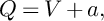 $Q=V+a,$
where V is the r-dimensional vector subspace of
 $E^{n-1}$
and a is a vector in Q. By Corollary 5.23, we have
 $$\begin{align*}\Lambda^{bl}(\Gamma_{p}) \subset \{ (p, \frac{v}{|v|}) \in \operatorname{Bl}_{p}(\mathbb{R}^{n}): v \in V\backslash \{0\} \}.\end{align*}$$
Conversely, for
 $v\in V\backslash \{0\}$
and any integer
 $n>0$
, there is an element
 $\gamma _{n}$
of
 $\Gamma _{\infty }$
such that
 $\gamma _{n} a \in N(nv+a, R),$
where R is the Euclidean diameter of a fundamental domain of Q for
 $\Gamma _{\infty }.$
By Lemma 5.22,
 $$\begin{align*}\lim_{n\rightarrow \infty} \gamma_{n}a = (p, \frac{v}{|v|}) \in \Lambda^{bl}(\Gamma_{p}).\end{align*}$$
Hence, we have
 $$\begin{align*}\Lambda^{bl}(\Gamma_{p}) = \{ (p, \frac{v}{|v|}) \in \operatorname{Bl}_{p}(\mathbb{R}^{n}): v\in V\backslash \{0\}\} \cong S^{r-1}.\end{align*}$$
Second, we show that
 $\Lambda ^{bl}(\Gamma ) \cap \pi _{C}^{-1}(p) =\Lambda ^{bl}(\Gamma _{p}).$
Let a be a point in
 $\Lambda ^{bl}(\Gamma ) \cap \pi _{C}^{-1}(p).$
There exist a point
 $x\in B^{n}$
and a sequence
 $\{g_{i}\}$
of
 $\Gamma $
such that
 $\displaystyle a=\lim _{n\rightarrow \infty } g_{i}x.$
If the sequence
 $\{g_{i}\}$
has infinitely many elements of
 $\Gamma _{p}$
, by the definition of
 $\Lambda ^{bl}(\Gamma _{p})$
, we have
 $a\in \Lambda ^{bl}(\Gamma _{p}).$
Otherwise, there exists a proper cusped region
 $U(Q, r)$
such that
 $g_{i}x \in N(Q,r)$
for infinitely many
 $i\in \mathbb {N}.$
By Corollary 5.23, a is in
 $\Lambda ^{bl}(\Gamma _{p}).$
Hence, we have
 $\Lambda ^{bl}(\Gamma ) \cap \pi _{C}^{-1}(p) \subset \Lambda ^{bl}(\Gamma _{p}).$
The converse inclusion is obvious.
Lemma 5.25. For any
 $x\in B^{n}$
,
 $$\begin{align*}\Lambda^{bl}(\Gamma) = \overline{\Gamma x} \cap \partial B^{bl}.\end{align*}$$
In particular, the blown-up limit set of
 $\Gamma $
is a
 $\Gamma $
-invariant closed subset of
 $B^{bl}$
.
Proof. By the definition of
 $\Lambda ^{bl}(\Gamma )$
, it is obvious that
 $\Lambda ^{bl}(\Gamma ) \supset \overline {\Gamma x} \cap \partial B^{bl}.$
Conversely, for any
 $a\in \Lambda ^{bl}(\Gamma )$
, we put
 $\overline {a}=\pi _{C}(a) \in \Lambda (\Gamma )$
. If
 $\overline {a}$
does not lie in the set C of cusped limit points of
 $\Gamma $
, we can show that a is a limit point of
 $\Gamma $
in
 $\partial B^{bl}$
in the same way as a limit point of
 $\Gamma $
in
 $\partial B^{n-1}$
. If
 $a\in C$
, applying Lemma 5.24 to the cusped limit point a,
 $$\begin{align*}a \in \Lambda^{bl}(\Gamma)\cap \pi^{-1}_{C}(\overline{a}) = \Lambda^{bl}(\Gamma_{\overline{a}}) = \overline{\Gamma_{\overline{a}}x}\cap \partial B^{bl} \subset \overline{\Gamma x}\cap \partial B^{bl}. \end{align*}$$
Therefore,
 $\Lambda ^{bl} (\Gamma ) \subset \overline {\Gamma x}\cap \partial B^{bl}.$
Lemma 5.26. Let
 $\Gamma $
be a non-elementary geometrically finite subgroup of
 $M(B^{n})$
. Then,
 $$\begin{align*}\Lambda^{bl}(\Gamma) = \operatorname{St}_{C}(\Lambda(\Gamma)).\end{align*}$$
Proof. By Lemma 5.25, we have
 $\Lambda ^{bl}(\Gamma ) \subset \overline {\pi ^{-1}_{C}(\Lambda (\Gamma )\backslash C)} = \operatorname {St}_{C}(\Lambda (\Gamma )).$
Conversely, it is enough to show that
 $ \operatorname {St}_{C}(\Lambda (\Gamma )) \cap \pi ^{-1}_{C}(p) \subset \Lambda ^{bl}(\Gamma _{p}) $
for each
 $p \in C.$
By conjugating
 $\Gamma $
in
 $M(B^{n})$
, we can suppose
 $p=e_{n}$
. As a similar way in Lemma 5.24, we pass the upper half-space model
 $U^n$
, and
 $\Gamma $
acts on
 $U^n$
. Let
 $U(Q,r)$
be a proper cusped region for
 $\Gamma _{\infty }$
based at
 $\infty $
, where Q is a
 $\Gamma _{\infty }$
-invariant r-plane of
 $E^{n-1}$
such that
 $Q/\Gamma _{\infty }$
is compact. Then,
 $\Lambda (\Gamma ) \subset N(Q, r) \cup \{\infty \}.$
There exist a vector subspace V of
 $E^{n-1}$
and a vector a of Q such that
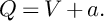 $Q=V+a.$
By Corollary 5.23 and Lemma 5.24, we have
 $$\begin{align*}\operatorname{St}_{C}(\Lambda(\Gamma)) \cap \pi^{-1}_{C}(p) \subset \big\{(e_{n}, \frac{v}{|v|}) : v\in V\backslash \{0\}\big\} = \Lambda^{bl}(\Gamma_{p}).\\[-42pt] \end{align*}$$
Definition 5.27. Let X be an algebraic K3 surface with
 $\rho (X) \geq 3$
, and let V (resp.
 $V_{X}$
) be the same as in Definition 5.10. We denote the strict transform of
 $\partial A_{X}$
(resp.
 $\overline {A_{X}}$
) at
 $V_{X}$
by
 $\partial A_{X}^{bl}$
(resp.
 $\overline {A_{X}}^{bl}$
). We call
 $\partial A_{X}^{bl}$
the blown-up boundary associated with the ample cone of X.
The following result is given by Baragar [Reference Baragar3]. By using the geometrical finiteness of
 $O^{+}(NS(X))$
, we can give another proof of the result.
Theorem 5.28 [Reference Baragar3, Theorem 3.3]
For an algebraic K3 surface X with
 $\rho (X)\geq 3$
, the set
 $\partial A_{X} \backslash \Lambda _{X}$
is equal to
 $V\backslash V_{X} =\{c\in V: \operatorname {Aut}(A(X))_{c} {\text { is finite}}\}.$
Proof. Let x be a point of
 $A_{X}.$
For any
 $y \in \partial A_{X}$
, we denote the hyperbolic line connecting x to y by
 $l_{x,y}.$
Let P be the Dirichlet domain of
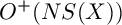 $O^{+}(NS(X))$
centered at x. Then, there exists a horoball
 $U(c)$
based at c such that:
-
(1)
$\{ \overline {U(c)} : c \in V_{NS}\}$
are mutually disjoint; -
(2)
$gU(c) = U(gc)$
for any element
$g \in O^{+}(NS(X))$
; -
(3)
$\{\overline {U(c)}\backslash {c} \} $
is locally finite in
$\mathbb {H}^{n}_{X}$
,




where the set
 $V_{NS}$
is the same as in Definition 5.10. Let V and
 $V_{X}$
be as in Definition 5.10. We put
 $K= \overline {P}\backslash \bigcup _{c\in V}U(c).$
Then, by Lemma 5.9,
 $\overline {A_{X}}^{H}\backslash \bigcup _{c\in V}U(c) = \operatorname {Aut}(A(X))\cdot K.$
If
 $y\notin V$
, since cusped regions
 $\{U(c): c\in V_{NS}\}$
are mutually disjoint, there exists a sequence
 $\{a_{n}\}_{n\in \mathbb {N}}$
and
 $\gamma _{n} \in \operatorname {Aut}(A(X))$
such that
 $a_{n}$
converges to infinity as
 $n\rightarrow \infty $
and
 $ l_{x,y}(a_{n}) \in \gamma _{n}K.$
Since the Euclidean diameter of
 $\gamma _{n}K$
goes to zero as n goes to infinity, we have
 $\displaystyle y =\lim _{n\rightarrow \infty }l_{x,y}(a_{n}) =\lim _{n\rightarrow \infty }\gamma _{n}x \in \Lambda _{X}.$
If
 $y\in V\backslash V_{X}$
and the rank of the stabilizer group
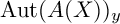 $\operatorname {Aut}(A(X))_{y}$
is 0, by Lemma 5.12, the point y is isolated in
 $\partial A_{X}.$
In particular, y is not in the limit set
 $\Lambda _{X}$
.
Otherwise, y is in
 $V_{X}$
. Since
 $V_{X} = \{c \in V : \operatorname {vcd} \operatorname {Aut}(X)_{c} \geq 1 \},$
y is a bounded parabolic limit point. In particular, y is in the limit set
 $\Lambda _{X}.$
Definition 5.29. Let X be an algebraic K3 surface with
 $\rho (X)\geq 3$
. In Definition 5.11, we defined the limit set
 $\Lambda _{X}$
of X. We denote the blown-up limit set of
 $\operatorname {Aut}_{s}(X)$
by
 $\Lambda _{X}^{bl}.$
Corollary 5.30. If the symplectic automorphism group
 $\operatorname {Aut}_{s}(X)$
of an algebraic K3 surface X with
 $\rho (X)\geq 3$
is non-elementary, then
 $\partial A_{X}^{bl}\backslash \Lambda ^{bl}_{X}= V\backslash V_{X}.$
Proof. By Theorem 5.28, we have
 $\partial A_{X}\backslash V = \Lambda (\Gamma ) \backslash V_{X}.$
Then, by Lemma 5.26, we have the desired equality.
Let C be the set of cusped limit points of
 $\operatorname {Aut}(A(X))$
. Since
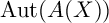 $\operatorname {Aut}(A(X))$
is geometrically finite, C is equal to
 $V_{X}$
. By Lemma 5.15, shrinking the horoballs
 $U(c)$
sufficiently small, there exist haroballs
 $U(c)$
based at
 $c \in C$
such that:
-
(1)
$\{U(c) :c\in C\}$
are mutually disjoint; -
(2)
$gU(c) = U(gc)$
for any
$g\in \operatorname {Aut}(A(X))$
and
$c\in C;$
-
(3)
$\{\overline {U(c)}\backslash \{c\}\}$
is locally finite in
$B^{n}$
; -
(4)
$U(c)$
meets just the sides of
$\overline {A_{X}}$
incident with c.



Since a horoball
 $U(c)$
is homeomorphic to its strict transformation on
 $\overline {B}^{bl}$
, we identify
 $U(c)$
with its strict transformation. To apply the Bestvina–Mess formula (Theorem 4.10) to automorphism groups of K3 surfaces, we construct a homotopy on
 $\overline {A_{X}}^{bl}\backslash \cup _{c\in C}U(c)$
.
Lemma 5.31. Let a be a point of
 $A_{X}$
, and let
 $K(a, t) = C(a, t) \cap \overline {A_{X}}\backslash \cup _{c\in C} U(c),$
where
 $C(a, t)$
is the closed t-ball centered at a. For every
 $x \in \overline {A_{X}}\backslash (\cup _{c\in C} U(c)\cup C),$
let
 $S_{x}$
be the smallest (horo)sphere (based) centered at x that meets
 $K(a, t)$
. Then,
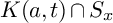 $K(a, t) \cap S_{x}$
is a singleton.
Proof. Suppose that there exists
 $y_{1}, y_{2}$
in
 $K(a, t)\cap S_{x}$
with
 $y_{1}\neq y_{2}.$
Then, the hyperbolic line
 $\lbrack y_{1}, y_{2} \rbrack $
connecting
 $y_{1}$
to
 $y_{2}$
is contained in
 $C(a, t)\cap \overline {A_{X}}.$
For any
 $z\in (y_{1}, y_{2})$
, we have
 $d(x,z) < d(x, y_{1}) = d(x, y_{2}).$
Then, we have
 $z \in \cup _{c\in C}U(c).$
Since horoballs
 $U(c)$
are mutually disjoint, there exists
 $c\in C$
such that
 $(y_{1}, y_{2}) \subset U(c)$
and
 $y_{1}, y_{2} \in K(a,t) \cap \partial U(c).$
We now pass to the upper half-space model
 $U^{n}$
and conjugate
 $\operatorname {Aut}(A(X))$
so that
 $c=\infty .$
We denote by
 $\Sigma $
(resp.
 $w_{1}, w_{2}$
) the horoball (resp. the point) on
 $U^n$
corresponding to
 $\partial U(c)$
(resp.
 $y_{1}, y_{2}$
). By Lemma 5.15, the Euclidean segment l connecting
 $y_{1}$
to
 $y_{2}$
is contained in
 $K(a,t)\cap \Sigma .$
This contradicts the minimality of
 $S_{x}$
.
Definition 5.32. Let
 $K(a,t)$
be the same as in Lemma 5.31. We put
 $$\begin{align*}U = \cup_{c\in C} U(c)\cup C.\end{align*}$$
For every
 $x \in \overline {A_{X}}\backslash U$
and
 $t\geq 0$
, we define the function
 $ \rho _{a}: \overline {A_{X}}\backslash U \times \lbrack 0, \infty ) \rightarrow \overline {A_{X}}\backslash U$
as follows: if
 $x\in K(a, t)$
, we define
 $\rho _{a}(x, t) = x,$
otherwise, we define
 $\rho _{a}(x, t)$
by the unique point of
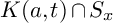 $K(a, t) \cap S_{x}$
.
In the case
 $t=0$
, for any
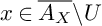 $x\in \overline {A_{X}}\backslash U$
, we have
 $\rho _{a}(x, 0)=a$
. Then, the restriction of
 $\rho _{a}$
at
 $t=0$
is a constant map.
Proposition 5.33. Let
 $\rho _{a}$
be the same as above. Then,
 $\rho _{a}$
is continuous.
Proof. If
 $\rho _{a}$
is not continuous, there exists a sequence
 $\{(x_{n}, t_{n})\}$
such that
 $(x_{n}, t_{n})$
converges to
 $(x, t)$
and
 $\rho _{a}(x_{n}, t_{n})$
converges to
 $y\neq \rho _{a}(x, t).$
If x is in
 $B^{n}$
, passing to a subsequence of
 $\{(x_{n}, t_{n})\}$
, we can assume that each
 $x_{n}$
is in
 $B^{n}$
. By the definition of
 $\rho _{a}(x_{n}, t_{n})$
(resp.
 $\rho _{a}(x, t)$
), there exists
 $r_{n}$
(resp. r) such that
 $S(x_{n}, r_{n}) \cap K(a, t_{n}) = \{ \rho _{a}(x_{n}, t_{n}) \}$
(resp.
 $S(x, r) \cap K(a, t) = \{ \rho _{a}(x, t) \}$
). Passing to a subsequence of
 $(x_{n}, t_{n})$
, we can suppose that
 $r_{n}$
converges to
 $r_{0}$
. Since
 $d((x_{n}, \rho _{a}(x_{n}, t_{n}))= r_{n}$
, we have
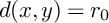 $d(x, y) = r_{0}$
. By the definition of
 $\rho _{a}(x, t)$
, we obtain
 $r_{0}>r$
. Hence, for a sufficiently large n, we have
 $r_{n}> d(x_{n}, \rho _{a}(x_{n}, t_{n})).$
This contradicts the definition of
 $r_{n}$
.
If x is in
 $\partial B^{n}$
, passing to the upper half-space model
 $U^n$
, there exists a (horo)sphere
 $S_{k}$
of
 $U^n$
(based) centered at
 $x_{k}$
such that
 $S_{k}\cap K(a, t_{k}) = \{\rho _{a}(x_{k}, t_{k})\}.$
We denote the Euclidean center (resp. radius) of
 $S_{k}$
by
 $p_{k}=(p_{k,1}, \cdots , p_{k,n})$
(resp.
 $r_{k}$
). Then, we have that
 $|p_{k}-\rho _{a}(x_{k}, t_{k})| = r_{k}$
,
 $|x_{k}-p_{k}|\leq r_{k}$
, and
 $r_{k} \leq p_{k, n}$
, where
 $| \hspace {2mm}|$
is the Euclidean norm. Passing to a subsequence of
 $\{(x_{n}, t_{n})\}$
, we can assume that
 $p_{k}$
(resp.
 $r_{k}$
) converges to some point
 $p=(p_{1}, \cdots , p_{n})$
(resp.
 $r\geq 0$
). As k goes to infinity, we have
 $$\begin{align*}|p-y| = r,\hspace{2mm} |x-p| \leq r,\hspace{2mm}{\text{and }} r \leq p_{n}. \end{align*}$$
Since x is in
 $\partial B^{n}$
, we have that
 $p=(x_{1}, \cdots , x_{n-1}, r)$
and
 $|x-p|=r$
. Since
 $|p-y|=r$
, this contradicts the uniqueness of
 $\rho _{a}(x,t)$
.
Proposition 5.34.
 $\rho _{a}$
extends to
 $\overline {\rho _{a}}: \overline {A_{X}}^{bl} \backslash \cup _{c\in C} U(c) \times \lbrack 0, \infty ) \rightarrow \overline {A_{X}}^{bl} \backslash \cup _{c\in C} U(c) $
.
Proof. Let x be a point in
 $\overline {A_{X}}^{bl} \backslash \cup _{c\in C} U(c)$
with
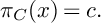 $\pi _{C}(x)=c.$
We now pass to the upper half-space model
 $U^n$
so that
 $a=e_{n}$
and
 $c=\infty $
by an isometry
 $\phi : B^{n}\rightarrow U^{n}.$
Let
 $\Sigma $
be the horosphere
 $\{x\in U^n: x_{n}=r\}$
based at
 $\infty $
corresponding to
 $U(c).$
If
 $K(a,t)\cap \Sigma = \varnothing $
or a singleton, we define
 $\overline {\rho _{a}}(x, t)$
by the point of
 $K(a, t)$
whose n-th element is maximal in
 $K(a, t).$
Otherwise, by Lemma 5.15,
 $\overline {A_{X}}\cap \Sigma $
is a
 $(n-1)$
-dimensional Euclidean polyhedron, and
 $K(a, t) \cap \Sigma $
is a convex subset of
 $\Sigma $
. Here, there exists the half-line
 $l_{x}$
on
 $\Sigma $
starting at
 $re_{n}$
such that
 $\operatorname {St}_{C}(\phi ^{-1} \circ l)\cap \pi _{C}^{-1}(c) = \{x\}.$
For any
 $t\geq 0$
, there exists a sufficiently large
 $R_{t}>0$
such that
 $\rho _{a}(x, s)$
is in
 $\Sigma $
for any
 $s\in (0, t\rbrack $
and any x with
 $|x|>R_{t}$
. Then, if we define
 $\overline {\rho _{a}}(x, t)$
by the intersection of
 $K(a, t)$
with
 $l_{x},$
this is the desired extension of
 $\rho _{a}.$
Theorem 5.35. Let X be an algebraic K3 surface with
 $\rho (X)\geq 3$
. If
 $\operatorname {Aut}_{s}(X)$
is non-elementary, then
 $(\overline {A_{X}}^{bl}\backslash \cup _{c\in C} U(c), \partial A_{X}^{bl})$
is a
 $\mathcal {Z}$
-structure for some torsion-free subgroup of
 $\operatorname {Aut}(X)$
of finite index. In particular,
 $$\begin{align*}\operatorname{vcd}(\operatorname{Aut}(X)) = \dim \partial A_{X}^{bl} + 1.\end{align*}$$
Proof. See Definition 4.9 for a
 $\mathcal {Z}$
-structure, and Theorem 4.10. By Selberg’s Lemma, there exists a torsion-free subgroup
 $\Gamma $
of
 $\operatorname {Aut}(X)$
of finite index. It suffices to verify that
 $\Gamma $
satisfies the conditions (1), (2), and (3) in Definition 4.9. As for the condition (2), since
 $\Gamma $
is torsion-free and its action on
 $\mathbb {H}_{X}^{n}$
is discontinuous, then this action is a covering space action. The compactness of
 $(\overline {A_{X}}\backslash \cup _{c\in C} U(c))/\Gamma $
can be concluded from that of
 $(\overline {A_{X}}\backslash \cup _{c\in C} U(c))/\operatorname {Aut}(X)$
. The condition (3) immediately follows from the Lebesgue Covering Lemma. Therefore, the essential part of the proof is to show that
 $\partial A_{X}^{bl}$
is a
 $\mathcal {Z}$
-set of
 $\overline {A_{X}}^{bl}\backslash \cup _{c\in C} U(c).$
We define the homotopy
 $H: (\overline {A_{X}}^{bl} \backslash \cup _{c\in C} U(c)) \times \lbrack 0, 1\rbrack \rightarrow \overline {A_{X}}^{bl} \backslash \cup _{c\in C} U(c)$
setting
 $$\begin{align*}H(t, x) = \left\{ \begin{array}{ll} (x, t) & (t=1) \\ \rho_{a}(x, \log{\frac{1+t}{1-t}}) & (t\neq 1). \end{array} \right.\end{align*}$$
By Proposition 5.34 and the definition of
 $\rho _{a}$
, H is continuous. Hence,
 $\partial A_{X}^{bl}$
is a
 $\mathcal {Z}$
-set of
 $\overline {A}_{X}^{bl}\backslash \cup _{c\in C} U(c)$
. Then,
 $(\overline {A}_{X}^{bl}\backslash \cup _{c\in C} U(c), \partial A_{X}^{bl})$
is a
 $\mathcal {Z}$
-structure for
 $\Gamma $
. By Theorem 4.10, we have the desired equality.
Corollary 5.36. If
 $\Lambda _{X}$
is homeomorphic to a Cantor set and X has an elliptic fibration whose rank is larger than
 $0$
, then
 $$\begin{align*}\operatorname{vcd}(\operatorname{Aut}(X)) = \max \operatorname{MW}(f:X\rightarrow \mathbb{P}^{1}), \end{align*}$$
where f runs all the elliptic fibrations of X.
Proof. For any
 $c\in C$
, we have
 $\Lambda ^{bl}_{X} \cap \pi _{C}^{-1}(c) \cong S^{r-1},$
where r is the rank of
 $\operatorname {Aut}(A(X))_{c}$
. By Proposition 5.16, r is equal to the rank of the Mordell weil group corresponding to c. If
 $c \notin C$
, since
 $\Lambda _{X}$
is totally disconnected,
 $\{c\}$
itself is an open neighborhood. Then, the topological dimension of
 $\Lambda ^{bl}_{X}$
is equal to
 $\max \operatorname {MW}(f:X\rightarrow \mathbb {P}^{1})$
.
Example 5.37. Let X be the K3 surface whose Néron–Severi lattice
 $NS(X)$
is given by
 $$\begin{align*}NS(X) = \begin{pmatrix} 2 & 4 & 1 \\ 4 & 2 & 0 \\ 1 & 0 & -2\\ \end{pmatrix}. \end{align*}$$
Baragar [Reference Baragar4] studied the automorphism group of this K3 surface and the growth of orbits of curves. He showed that
 $\Lambda _{X}$
is a Cantor set and
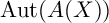 $\operatorname {Aut}(A(X))$
is isomorphic to
 $\mathbb {Z}/2\mathbb {Z} *\mathbb {Z}/2\mathbb {Z} *\mathbb {Z}/2\mathbb {Z}.$
Although the automorphism group of X is completely determined in [Reference Baragar4] as above and then this is not a new example of computing the virtual cohomological dimensions, we can also apply Corollary 5.36 to this K3 surface X.
5.3 The ample cones of K3 surfaces and sphere packings
Let X be a K3 surface, and let
 $\phi : \mathbb {H}_{X}^{n} \rightarrow B^n$
be an isometry from
 $\mathbb {H}_{X}^{n}$
to the conformal ball model
 $B^n$
. The isometry
 $\phi $
induces the natural homeomorphism from
 $\partial \mathbb {H}_{X}^{n}$
to
 $\partial B^n.$
For a root
 $\delta $
and an ample class a of X, we set
 $$ \begin{align*} H_{\delta}&=\{x \in \mathbb{H}_{X}^{n}: d(x,a)=d(x, s_{\delta}a)\}, \\ H_{\delta}^{+}&= \{x \in \mathbb{H}_{X}^{n}: d(x,a)<d(x, s_{\delta}a)\}. \end{align*} $$
The closure of
 $H_{\delta }$
(resp.
 $H_{\delta }^{+}$
) in
 $\overline {\mathbb {H}_{X}^n}$
is denoted by
 $\overline {H_{\delta }}$
(resp.
 $\overline {H}_{\delta }^{+}$
). We set
 $$\begin{align*}\mathcal{S}_{X}= \lbrace \delta \in \Delta^{+}(X): H_{\delta}\cap \overline{A_{X}}^{H} {\text{ is a side of }} \overline{A_{X}}^{H} \rbrace,\end{align*}$$
where
 $\overline {A_{X}}^{H}$
is the closure of
 $A_{X}$
in
 $\mathbb {H}_{X}^{n}.$
Definition 5.38. Let
 $\delta $
be an element of
 $\mathcal {S}_{X}$
. We define the sphere associated with
 $\delta $
by
 $S_{\delta }= \phi (\overline {H_{\delta }})\cap \partial B^{n}$
, which is isomorphic to the
 $(n-2)$
-sphere. We define
 $B_{\delta }=\phi (\overline {H}_{\delta }^{+}\backslash \overline {H_{\delta }})\cap \partial B^n.$
We call
 $B_{\delta }$
the open ball associated with
 $\delta $
.
By Proposition 5.7, we have
 $ A_{X} = \cap _{\delta \in \mathcal {S}_{X}} H_{\delta }^{+}$
and
 $\partial A_{X} = \cap _{\delta \in \mathcal {S}_{X}} \overline {B_{\delta }},$
where
 $\overline {B_{\delta }}$
is the closure of
 $B_{\delta }$
in
 $\partial B^n.$
Definition 5.39. The boundary
 $\partial A_{X}$
associated with the ample cone of X is a sphere packing if for any two different
 $\delta _{1}$
,
 $\delta _{2}$
in
 $\mathcal {S}_{X}$
, their associated spheres
 $S_{\delta _{1}}$
and
 $S_{\delta _{2}}$
are either disjoint or tangent to each other.
 $\partial A_{X}$
is called a connected sphere packing if
 $\partial A_{X}$
is a sphere packing, and for any two different
 $\delta $
,
 $\delta ^{'}$
in
 $\mathcal {S}_{X}$
, there exist roots
 $\delta _{1}, \dots , \delta _{n}$
in
 $\mathcal {S}_{X}$
such that
 $\delta =\delta _{1}$
,
 $\delta ^{'}=\delta _{n}$
, and two spheres
 $S_{\delta _{i}}$
and
 $S_{\delta _{i+1}}$
are tangent for
 $i=1, \dots , n-1.$
Theorem 5.40. Let X be an algebraic elliptic K3 surface with
 $\rho (X)\geq 3$
. If
 $\partial A_{X}$
is a connected sphere packing, and every elliptic divisor of X corresponds to the tangent point of some two spheres associated with elements of
 $\mathcal {S}_{X}$
, then
 $$\begin{align*}\operatorname{vcd}(\operatorname{Aut}(X)) =\max \{ \operatorname{rk}\operatorname{MW}(f)\} =\rho(X)-3 ,\end{align*}$$
where f runs all elliptic fibrations of X.
Proof. As
 $\partial A_{X}$
is connected, we can sort the set of the open balls associated with elements of
 $\mathcal {S}_{X}$
to
 $\{ B_{i}\}_{i \in \mathbb {N}}$
such that for any
 $i\in \mathbb {N}$
, the intersection of
 $B_{i}$
with
 $\cup _{j=1}^{i-1}B_{j}$
is not empty. Let
 $\mathcal {P}_{m}$
be the set
 $\{p : p \in B_{i} \cap B_{j} {\text { for some two distinct }} i, j \leq m\}.$
We define the following sets:
-
•
$U_{m} = \bigcap _{i=1}^{m}B_{i}$
; -
•
$F_{m} = \bigcap _{i=1}^{m}\overline {B_{i}}$
; -
•
$F_{m}^{bl} =\operatorname {St}_{\mathcal {P}_{m}}(F_{m}) =$
the strict transform of
$F_{m}$
at
$\mathcal {P}_{m}$
.


For any
 $l<m$
, let
 $\pi _{\mathcal {P}_{l}, \mathcal {P}_{m}}$
be the same as in Definition 5.19. The map
 $\pi _{\mathcal {P}_{l}, \mathcal {P}_{m}}$
restricts to a map from
 $F_{m}^{bl}$
to
 $F_{l}^{bl}.$
These maps form a projective system. Since
 $\partial A_{X}$
is a subset of
 $F_{m}$
for any
 $m\in \mathbb {N},$
there exists the natural map
 $\phi _{m}:\partial A_{X}^{bl} \rightarrow F_{m}^{bl}$
. Then, we have the natural map
 $\phi : \partial A_{X}^{bl} \rightarrow \varprojlim F_{m}^{bl}$
. The map
 $\phi $
is a homeomorphism. To show this, we consider the following:
 $$\begin{align*}\psi_{m}: \varprojlim F_{i}^{bl} = \varprojlim \operatorname{St}_{\mathcal{P}_{i}}(F_{i}) \rightarrow \cap_{i \in \mathbb{N}} \operatorname{St}_{\mathcal{P}_{m}}(F_{i}) = \operatorname{St}_{\mathcal{P}_{m}}(\partial A_{X}) .\end{align*}$$
Since
 $\partial A_{X}^{bl}=\varprojlim \operatorname {St}_{\mathcal {P}_{m}}(\partial A_{X})$
, the maps
 $\psi _{m}$
induce the natural map
 $\psi : \varprojlim F_{m}^{bl}\rightarrow \partial A_{X}^{bl}$
, which is the inverse of
 $\phi .$
For each
 $m\in \mathbb {N}$
,
 $F_{m}^{bl}$
is a topological manifold with its interior
 $U_{m},$
and then
 $F_{m}^{bl}$
and
 $U_{m}$
are homotopy equivalent. Hence, we have
 $$ \begin{align} H^{*}(\partial A_{X}^{bl}, \mathbb{Z}) \cong \lim_{m \to \infty} H^{*}(F_{m}^{bl},\mathbb{Z}) \cong \lim_{m \to \infty} H^{*}(U_{m},\mathbb{Z}). \end{align} $$
For each
 $m \in \mathbb {N}$
and a sufficiently small
 $\epsilon>0$
, we define
 $V_{m+1}$
by the
 $\epsilon $
-neighborhood of
 $\partial B^{n} \backslash B_{m+1}$
in
 $U_{m}.$
Then, we can see as follows:
-
•
$V_{m+1}$
is contractible; -
•
$U_{m+1}\cup V_{m+1} = U_{m};$
-
•
$U_{m+1}\cap V_{m+1}$
is homotopy equivalent to the
$(n-2)$
-sphere with finite k punctures,




where k is the number of the set
 $\{p: p {\text { is a tangent point of }} B_{i} {\text { and }} B_{m+1} {\text { for some }} i\leq m\}.$
By Mayer–Vietoris exact sequence and the
 $(n-2)$
-sphere with k punctures is homotopy equivalent to the wedge sum of
 $(k-1)$
-copies of
 $S^{n-3}$
, we have the following exact sequence:
 $$\begin{align*}\cdots \rightarrow H^{*}(U_{m}) \rightarrow H^{*}(U_{m+1})\oplus H^{*}(V_{m+1}) \rightarrow H^{*}(\vee_{i=1}^{k-1} S^{n-3}) \rightarrow H^{*+1}(U_{m}) \rightarrow \cdots.\end{align*}$$
Therefore, we can inductively conclude that
 $$\begin{align*}H^{*}(U_{m}) = 0 \hspace{3mm}( *\geq n-2).\end{align*}$$
In particular, by Theorem 5.35 and the equation 5.4, we have
 $$ \begin{align*} \operatorname{vcd}\operatorname{Aut}(X) &= \max\{ m : H_{c}^{m}(\overline{A_{X}}^{H}\backslash \cup_{c\in C}U(c) , \mathbb{Z})\neq 0\} \\ &= \max\{ m : H^{m}(\partial A_{X}^{bl}, \mathbb{Z})\neq 0\}+1 \\ &\leq n-2 =\rho(X)-3, \end{align*} $$
where
 $H^{*}_{c}$
is the cohomology with compact support. Lemma 5.13 implies that there exists an elliptic fibration f such that
 $\operatorname {rk}\operatorname {MW}(f)= \rho (X)-3.$
Example 5.41. The Apollonian circle packing is generated as follows: we begin with four mutually tangent circles. There is four curvlinear triangles. We can put the inscribed circle for each curvlinear triangle, so that the curvlinear triangle separated into new curvlinear triangles. Inductively, we put inscribed circles for each curvelinear triangle, and the closure of the union of the inscribed circles is the Apollonian circle packing, which is shown in the following Figure 1.
The Apollonian circle packing.

Baragar [Reference Baragar2] constructed a K3 surface
 $Y_{2}$
with ample cone the Apollonian circle packing, whose Néron–Severi lattice is given by
 $$\begin{align*}\begin{pmatrix} -2 & 2 & 2 & 4 \\ 2 & -2 & 2 & 4 \\ 2& 2 & -2 & 0 \\ 4 & 4 & 0 & 0 \\ \end{pmatrix}. \end{align*}$$
By Theorem 5.40, we have
 $\operatorname {vcd} \operatorname {Aut}(Y_{2}) = 1.$
Example 5.42. The Apollonian sphere packing is the three-dimensional analog of the Apollonian circle packing. We begin with five mutually tangent spheres, and in the space between any four of them, we put the inscribed sphere. As the same manner in the previous example, we can inductively put a sphere so that this sphere touch other four spheres. The closure of the union of the inscribed spheres is the Apollonian sphere packing. Baragar [Reference Baragar2] also constructed a K3 surface
 $Y_{3}$
with ample cone the Apollonian sphere packing, whose Néron–Severi lattice is given by
 $$\begin{align*}\begin{pmatrix} -2 & 2 & 2 & 2 & 4 \\ 2 & -2 & 2 & 2 & 4 \\ 2 & 2 & -2 & 2 & 4 \\ 2 & 2 & 2 &-2 & 0 \\ 4 & 4 & 4 &0 & 0 \\ \end{pmatrix}. \end{align*}$$
By Theorem 5.40, we have
 $\operatorname {vcd}\operatorname {Aut}(Y_{3}) = 2.$
6 Counterexamples to Mukai’s conjecture for elliptic K3 surfaces
In this section, we construct counterexamples to Mukai’s conjecture for elliptic K3 surfaces. Namely, we use hyperbolic geometry to construct the Néron–Severi lattice of K3 surfaces such that the virtual cohomological dimension of its automorphism group is equal to 1, while the maximal rank of Mordell–Weil groups is equal to 0.
6.1 A Transformation from the upper half-plane to the hyperboloid model
To study the action of the automorphism group of a K3 surface on the upper half-plane
 $U^2$
, we construct a standard transform from
 $U^2$
to the hyperboloid model of the hyperbolic plane.
Let
 $U^2$
be the upper half-plane. It is well-known that it can be identified with the subset of
 $\mathbb {C}$
consisting of elements with a positive imaginary part, and the group of linear fractional transformations corresponds to the group of orientation-preserving isometries of
 $U^2$
. Moreover, there exists an isometry from
 $U^2$
to the conformal ball model
 $B^2$
of the hyperbolic plane defined by
 $$\begin{align*}\sigma: U^2 \rightarrow B^2: z \mapsto \frac{z-i}{z+i}, \end{align*}$$
where i is the imaginary unit. Here
 $\sigma $
is called the Cayley transform. Let
 $V^{1,2}$
be a 3-dimensional vector space with the inner product
 $\langle \hspace {1mm}, \hspace {1mm} \rangle $
, where
 $\langle x, x\rangle = x_{0}^2-x_{1}^2-x_{2}^2$
for
 ${x=(x_{0}, x_{1}, x_{2}) \in V^{1,2}.}$
Then, the hyperboloid model
 $H^2$
associated with
 $V^{1,2}$
is defined by
 $$\begin{align*}H^2 = \{ x \in V^{1,2}: \langle x, x \rangle = 1, x_{0}>0\}.\end{align*}$$
The stereographic projection
 $\zeta $
is defined by the formula
 $$\begin{align*}\zeta(x) =(\frac{1+\| x\|^2}{1-\|x\|^2}, \frac{2x_{1}}{1-\|x\|^2}, \frac{2x_{2}}{1-\|x\|^2}).\end{align*}$$
Here, the map
 $\zeta \circ \sigma : U^2 \rightarrow H^{2}$
is an isometry from
 $U^2$
to
 $H^2$
. This map can be extended to
 $\overline {U^2}$
to
 $\overline {H^2}$
, also denoted by
 $\zeta \circ \sigma .$
Let us recall that
 $\partial U^2=\mathbb {R}$
and
 $\partial H^2=\{x\in V^{1,2}: \langle x, x \rangle =0, x_{0}>0\}/\mathbb {R}_{>0}.$
Then, for every
 $x\in \mathbb {R}$
, we have
 $\sigma (x) = (\frac {x^2-1}{x^2+1}, \frac {-2x}{x^2+1})$
, and we may take the point
 $(1, \frac {x^2-1}{x^2+1}, \frac {-2x}{x^2+1})$
as a representative of the class of
 $\zeta \circ \sigma (x).$
Here, we fix a positive real number k. Considering the set
 $\{ k^n : n\in \mathbb {Z}\},$
and the geodesics of
 $U^2$
connecting
 $k^n$
to
 $k^{n+1}$
, we have the following Figure 2.
Geodesics connectiong
 $k^n$
to
 $k^{n+1}$
 $(k = -1, 0, 1)$
.

From now on, we will construct the Néron–Severi lattice of K3 surfaces whose elliptic divisors correspond to the points
 $k^n (n\in \mathbb {Z})$
, and
 $(-2)$
-curves correspond to geodesics connecting
 $k^n$
to
 $k^{n+1}.$
We define the isotropic vector
 $$\begin{align*}e_{n} = (1, \frac{k^{2n}-1}{k^{2n}+1}, \frac{-2k^{n}}{k^{2n}+1})\in V^{1,2},\end{align*}$$
which corresponds to
 $k^n.$
Next, let
 $\delta _{n}$
be the element of
 $V^{1,2}$
with
 $\delta _{n}^2=-2$
such that
 $\langle \delta _{n}, e_{n}\rangle = \langle \delta _{n}, e_{n+1}\rangle =0.$
Then, by the direct computation, we have
 $$\begin{align*}\delta_{n} = \pm (\frac{k^{2n+1}+1}{k^n(k-1)}\sqrt{2}, \frac{k^{2n+1}-1}{k^n(k-1)}\sqrt{2}, -\frac{k+1}{k-1}\sqrt{2}).\end{align*}$$
Here, we want
 $\delta _{n}$
to be an effective (
 $-$
2)-curve, so its intersection with
 $(1,0,0) \in V^{1,2}$
should be positive. Then, we define
 $$\begin{align*}\delta_{n} = (\frac{k^{2n+1}+1}{k^n(k-1)}\sqrt{2}, \frac{k^{2n+1}-1}{k^n(k-1)}\sqrt{2}, -\frac{k+1}{k-1}\sqrt{2}).\end{align*}$$
Let
 $L(m)$
be the group generated by
 $\delta _{1}$
,
 $\delta _{2}$
, and
 $\delta _{3}$
, where
 $m=k+\frac {1}{k}$
. Then, by the direct computation, the Gram matrix of
 $L(m)$
is given by
 $$\begin{align*}\begin{pmatrix} -2 & 2 & 6+4m \\ 2 & - 2 & 2 \\ 6+4m & 2 & -2 \end{pmatrix} .\end{align*}$$
In particular,
 $L(m)$
is a lattice when
 $m=k+\frac {1}{k}$
is an integer, so we assume
 $m\in \mathbb {Z}$
from now on.
Proposition 6.1. Let
 $m=k+\frac {1}{k}$
be a positive integer, and let
 $L(m)$
be the same as above. Then, we have
 $$\begin{align*}\delta_{n+3} = \delta_{n} -(m+1)\delta_{n+1} +(m+1)\delta_{n+2},\end{align*}$$
for any
 $n\in \mathbb {Z}.$
In particular, for any
 $n\in \mathbb {Z}$
,
 $\delta _{n}$
is an element of the lattice
 $L(m)$
.
Proof. This equality can be confirmed by a straightforward computation. However, we will provide a proof by using hyperbolic geometry.
Let v
1 = −δ
1 + δ
3, v
2 = −δ
2 + δ
3, v
3 = δ
1 − mδ
2 + δ
3. Then, the reflection
 $s_{i}$
associated with
 $v_{i}$
is defined by
 $$\begin{align*}s_{i}(u) =u- 2\frac{\langle v_{i}, u\rangle}{\langle v_{i}, v_{i}\rangle}v_{i}.\end{align*}$$
As for the reflection
 $s_{1}$
, we have
 $$ \begin{align*} \langle v_1, v_1 \rangle &= (-\delta_{1}+\delta_{2})^2= -4-2(6+4m)= -8(2+m), \\ \langle v_{1}, u \rangle & = \langle -\delta_{1}+\delta_{2}, x\delta_{1}+y\delta_{2}+z\delta_{3}\rangle =4(2+m)(x-z), \end{align*} $$
where
 $u=x\delta _{1}+y\delta _{2}+z\delta _{3}$
. Then,
 $s_{1}(u)= z\delta _{1} + y\delta _{2}+x\delta _{3},$
and so the matrix representation
 $A_{1}$
of
 $s_{1}$
with the basis
 $\delta _{1}, \delta _{2}$
and
 $\delta _{3}$
is given by
 $$\begin{align*}\begin{pmatrix} 0 & 0& 1 \\ 0 & 1 & 0 \\ 1 & 0 & 0 \end{pmatrix} .\end{align*}$$
Let
 $A_2, A_3$
be the matrix representations of
 $s_{2}, s_{3}$
with the same basis as above, respectively. Then, we have
 $$\begin{align*}A_2 = \begin{pmatrix} 1 & 0& 0 \\ -(1+m) & 0 & 1 \\ -(1+m) & 1 & 0 \end{pmatrix} , \hspace{2mm} A_3 = \begin{pmatrix} 1+\frac{2}{m-2} &\frac{2}{m-2} & \frac{2}{m-2} \\ -\frac{2m}{m-2} & 1-\frac{2m}{m-2} & - \frac{2m}{m-2} \\ \frac{2}{m-2} & \frac{2}{m-2} & 1+\frac{2}{m-2} \end{pmatrix} .\end{align*}$$
Here,
 $v_3$
is orthogonal to the vectors
 $(1,0,0), (0,1,0)\in V^{1,2}.$
Since the vectors
 $(1,1,0), (1,-1,0) \in V^{1,2}$
are representatives of
 $0, \infty \in U^2,$
then the set of fixed points of
 $s_3$
is equal to the positive part of the imaginary axis of
 $U^2$
. Therefore,
 $s_{3}$
acts on
 $U^2$
as the reflection with respect to the imaginary axis. In the same way, because
 $\langle v_2, \delta _2+\delta _3\rangle = \langle v_2, v_3\rangle = 0$
,
 $s_{2}$
is the reflection with respect to the geodesic which is orthogonal to the imaginary axis and passes through
 $k^3$
. Because
 $\langle v_{1}, \delta _{2}\rangle = \langle v_1, v_3 \rangle = 0$
,
 $s_{1}$
is the reflection with respect to the geodesic which is orthogonal to the imaginary axis and the geodesic defined by
 $\delta _2$
.
We set
 $\phi =s_{2}\circ s_{1}.$
Since
 $s_1, s_2$
are reflections with respect to semicircles centered at the origin,
 $\phi $
acts on
 $U^2$
as a multiplication by a scalar.
Since
 $\phi (\delta _2) =s_2(\delta _2) = \delta _3,$
comparing the endpoints of the geodesic defined by
 $\delta _2$
, we find
 $\phi (\{k^2, k^3\})=\{k^3, k^4\}.$
Therefore, the action of
 $\phi $
on
 $U^2$
is equal to the multiplication by k.
Let R be the matrix representation of
 $\phi $
. Then, we have
 $$\begin{align*}R= A_2A_1 = \begin{pmatrix} 0 & 0& 1 \\ 1& 0 & -(1+m)\\ 0 & 1 & (1+m) \end{pmatrix} .\end{align*}$$
Hence, we get
 $$\begin{align*}\delta_{4} = \delta_{1} -(m+1)\delta_{2} +(m+1)\delta_{3}.\end{align*}$$
Applying
 $\phi ^n$
to this equation, we have the desired equation.
From the above proof, we obtain the following proposition.
Proposition 6.2. Let
 $A_{1}, A_{2},$
and
 $A_{3}$
be as above. If
 $m=3$
or
 $4$
, then the matrices
 $A_{1}, A_{2},$
and
 $A_{3}$
are isometries of the lattice
 $L(m).$
Moreover, they induce isometries of the upper half-space
 $U^2$
.
6.2 Counterexamples
We will show that K3 surfaces whose Néron–Severi lattice is isomorphic to
 $L(3)$
, or
 $L(4)$
are counterexamples to Mukai’s conjecture.
Theorem 6.3. Let X be a K3 surface whose Néron–Severi lattice is isomorphic to
 $L(3)$
or
 $L(4)$
. Then, the virtual cohomological dimension of its automorphism group is equal to 1, whereas every Mordell–Weil group has rank 0.
Proof. In the case
 $m=3$
, we have
 $$\begin{align*}v_3 = (1, -3, 1), \hspace{2mm} L(3) = \begin{pmatrix} -2 & 2& 18 \\ 2& -2 &2\\ -18 & 1 & -2 \end{pmatrix} .\end{align*}$$
First, we show that any geodesics defined by (
 $-$
2)-elements do not intersect with the imaginary axis. Let
 $\delta =x\delta _1 +y\delta _2+ z\delta _3$
be such an element. Then, since
 $\langle \delta , v_3 \rangle = 0$
and
 $\delta ^2=-2$
, we have x + y + z = 0, x
2 + y
2 + z
2 − 2xy − 2yz − 18xz = 1. By eliminating y, we obtain
 $4(x^2+z^2-3xz)=1$
. This is a contradiction.
Let D be the fundamental domain for
 $W(X)$
on
 $U^2$
that contains the positive part of the imaginary axis. Since
 $A_{1}, A_{2},$
and
 $A_{3}$
preserve it, we have
 $A_{1}, A_2, A_3 \in \operatorname {Aut}(D).$
Then, some power of
 $\phi $
is an automorphism of X, and so
 $\operatorname {vcd}(\operatorname {Aut}(X))\geq 1.$
Here, the set of facets of D naturally corresponds to the set of (
 $-$
2)-elements
 $\delta _{n}$
and
 $s_{3}(\delta _{n})$
(
 $n\in \mathbb {Z}$
). Suppose the contrary. There exists a facet of D that separates some
 $k^m$
from D. Then, applying
 $\phi ^n$
and
 $s_3 \circ \phi ^n$
(
 $n\in \mathbb {Z}$
) to the facet, we can conclude that D does not contain any isotropic element of
 $L(3)$
. Since
 $\delta _{2}+\delta _{3}$
is isotropic, this is the contradiction that there exists
 $w\in W(X)$
such that
 $w(\delta _{2}+\delta _{3}) \in D$
. Therefore, the facets of D are defined by (
 $-$
2)-element
 $\delta _{n}$
and
 $s_{3}(\delta _n)$
 $(n\in \mathbb {Z})$
, and each
 $\pm k^n$
corresponds to an elliptic fibration. Since such an elliptic fibration has rank 0 by Shioda–Tate formula, the maximum rank of Mordell–Weil groups of X is equal to 0. The same holds for
 $m=4.$
Acknowledgements
First, the author expresses his gratitude to his supervisor Fumiharu Kato, for providing the interesting topics and for many helpful discussions. He is grateful to Shigeru Mukai for various useful advice on the virtual cohomological dimension of automorphism groups of K3 surfaces. He thanks Takefumi Nosaka, Ryokichi Tanaka, and Kohei Kikuta for valuable comments and careful reading this article. Finally, he thanks Tomohiro Fukaya for many useful comments on hyperbolic geometry and hyperbolic group theory.