1 Introduction
Force-free magnetic configurations satisfying the condition
 $$\begin{eqnarray}\displaystyle \boldsymbol{B}=\unicode[STIX]{x1D705}\boldsymbol{J}, & & \displaystyle\end{eqnarray}$$
where  $\boldsymbol{B}$ is magnetic field and
 $\boldsymbol{J}$ is current density, are examples of magnetic structures that may represent the final stages of magnetic relaxation, or can be used as building blocks of plasma models (Lundquist Reference Lundquist1951; Woltier Reference Woltier1958; Taylor Reference Taylor1974; Priest & Forbes Reference Priest and Forbes2000).
Particular linear examples of force-free equilibria, with spatially constant  $\unicode[STIX]{x1D705}$, were considered by Chandrasekhar & Kendall (Reference Chandrasekhar and Kendall1957). The most often-used configurations are Lundquist fields in cylindrical geometry (Lundquist Reference Lundquist1951) and spheromaks in spherical geometry (Bellan Reference Bellan2000).
Using the self-similar assumption, Lynden-Bell & Boily (Reference Lynden-Bell and Boily1994) (see also Aly Reference Aly1994) found nonlinear self-similar solutions in spherical geometry. Their model of axially symmetric twisted configurations has been widely used in astrophysical and space applications (e.g. Thompson, Lyutikov & Kulkarni Reference Thompson, Lyutikov and Kulkarni2002; Shibata & Magara Reference Shibata and Magara2011). In the spirit of Lynden-Bell & Boily (Reference Lynden-Bell and Boily1994), in this paper we construct similar nonlinear magnetic configurations in cylindrical geometry.
2 Self-similar configuration in cylindrical geometry
Shafranov (Reference Shafranov1966) and Grad (Reference Grad1967) formulated what is known as the Grad–Shafranov equation, separating a complicated magnetic configuration in the set of nested/foliated flux surfaces, given by the condition that the flux function  $P$ is constant on the surface, and the encompassed current flow. Let us look for force-free equilibria that are independent of the coordinate
 $z$. The two Euler potentials
 $\unicode[STIX]{x1D6FC}$ and
 $\unicode[STIX]{x1D6FD}$ (or, equivalently, the related Clebsh variables) are
 $$\begin{eqnarray}\displaystyle \left.\begin{array}{@{}c@{}}\unicode[STIX]{x1D6FC}=z,\\ \unicode[STIX]{x1D6FD}=P(r,\unicode[STIX]{x1D719}),\end{array}\right\} & & \displaystyle\end{eqnarray}$$
while the magnetic field can be written as
 $$\begin{eqnarray}\displaystyle \boldsymbol{B}=\unicode[STIX]{x1D735}P\times \unicode[STIX]{x1D735}z+g(P)\unicode[STIX]{x1D735}z, & & \displaystyle\end{eqnarray}$$
where  $g$ is some function.
Next we introduce a self-similar ansatz
 $$\begin{eqnarray}\displaystyle \left.\begin{array}{@{}c@{}}P(r,\unicode[STIX]{x1D719})=r^{-l}f(\unicode[STIX]{x1D719}),\\ g(P)={\mathcal{C}}|P|^{p},\\ \boldsymbol{B}=\unicode[STIX]{x1D735}P\times \unicode[STIX]{x1D735}z+{\mathcal{C}}|P|^{p}\unicode[STIX]{x1D735}z=\{f^{\prime },lf,{\mathcal{C}}|f|^{p}\}r^{-(l+1)}.\end{array}\right\} & & \displaystyle\end{eqnarray}$$
The absolute value of  $|P|$ in the nonlinear term ensures that magnetic field is real (
 $f(\unicode[STIX]{x1D719})$ can become negative). Below, any appearance of
 $f$ to a non-integer power is to be understood to involve
 $\sqrt{f^{2}}=|f|$.
By dimensionality (equating radial powers in different terms in (1.1) with magnetic field given by (2.3)),
 $$\begin{eqnarray}\displaystyle p=1+1/l. & & \displaystyle\end{eqnarray}$$
The equation for  $f$ becomes
 $$\begin{eqnarray}\displaystyle lf^{\prime \prime }+l^{3}f+{\mathcal{C}}^{2}(1+l)f^{(2+l)/l}=0 & & \displaystyle\end{eqnarray}$$
(note that the component  $B_{z}$ enters here as
 $B_{z}^{2}$. This justifies the use of
 $|P|$).
For vacuum fields  ${\mathcal{C}}=0$, the above relations reproduce
 $$\begin{eqnarray}\displaystyle \left.\begin{array}{@{}c@{}}P\propto r^{-m}\sin (m\unicode[STIX]{x1D719}),\\ B_{r}\propto r^{-(1+m)}f^{\prime },\\ B_{\unicode[STIX]{x1D719}}\propto mr^{-(1+m)}f,\end{array}\right\} & & \displaystyle\end{eqnarray}$$
with integer  $m$.
The first integral is
 $$\begin{eqnarray}\displaystyle f^{\prime ,2}+l^{2}f^{2}+{\mathcal{C}}^{2}|f|^{2(1+l)/l}=H_{0}. & & \displaystyle\end{eqnarray}$$
By redefining  $f\rightarrow \sqrt{H_{0}}f$ and
 ${\mathcal{C}}\rightarrow {\mathcal{C}}H_{0}^{-1/(2l)}$, the parameter
 $H_{0}$ can be set to unity,
 $$\begin{eqnarray}\displaystyle f^{\prime ,2}+l^{2}f^{2}+{\mathcal{C}}^{2}|f|^{2(1+l)/l}=1. & & \displaystyle\end{eqnarray}$$
Equation (2.8) is the main equation describing nonlinear force-free structures in cylindrical geometry. It depends on one parameter – the current strength  ${\mathcal{C}}$. For a given
 ${\mathcal{C}}$, the value of
 $l$ is then determined as an eigenvalue problem by requiring periodicity in
 $\unicode[STIX]{x1D719}$, as we describe next.
We can solve for  $f$ in quadratures:
 $$\begin{eqnarray}\displaystyle \unicode[STIX]{x1D719}=\int (\sqrt{1-l^{2}f-{\mathcal{C}}^{2}|f|^{2(1+l)/l}})^{-1}\,\text{d}f & & \displaystyle\end{eqnarray}$$
(so that the integration constant in (2.8) is just a phase  $\unicode[STIX]{x1D719}$ where
 $f=0$).
Periodicity in  $\unicode[STIX]{x1D719}$ requires
 $$\begin{eqnarray}\displaystyle \int _{0}^{f_{\max }}(\sqrt{1-l^{2}f-{\mathcal{C}}^{2}|f|^{2(1+l)/l}})^{-1}\,\text{d}f=\frac{\unicode[STIX]{x03C0}}{2\tilde{m}}, & & \displaystyle\end{eqnarray}$$
where  $\tilde{m}=1,2\ldots$ is an integer azimuthal number (see a comment after (3.5) as to why odd solutions,
 $\propto 2\tilde{m}+1$, in the denominator, are discarded). The value of
 $f_{\max }$ satisfies
 $$\begin{eqnarray}\displaystyle 1-\tilde{m}^{2}f_{\max }-{\mathcal{C}}^{2}f_{\max }^{2(1+l)/l}=0. & & \displaystyle\end{eqnarray}$$
For given  ${\mathcal{C}}$, the relations (2.10)–(2.11) constitute an eigenvalue problem on
 $l$. (For the vacuum no-current case
 ${\mathcal{C}}=0$, this reduces to
 $l=2\tilde{m}$, an integer – as it should.) In practice, we follow the following procedure: for each
 $\tilde{m}=1,2,\ldots$, we assume some
 $l$ and find
 ${\mathcal{C}}$ using the relations (2.10)–(2.11). Thus, for each
 $m$, there is a continuous relation
 ${\mathcal{C}}(l)$. (Physically, of course, it is the current
 ${\mathcal{C}}$ that determines the radial index
 $l$.)
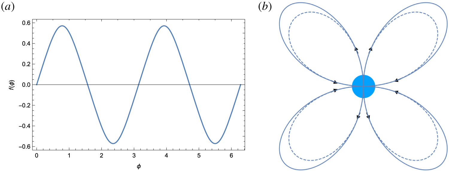
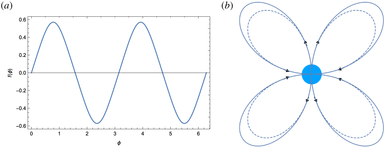
Results are plotted in figures 2 and 3. In figure 2 we plot a particular solution for  $l=1$ and
 $\tilde{m}=2$. The flux functions form a ‘petal’ pattern in azimuthal angle with the number of ‘petals’ equal to
 $2\tilde{m}$. There is a corresponding axial, unidirectional magnetic field
 $B_{z}$.
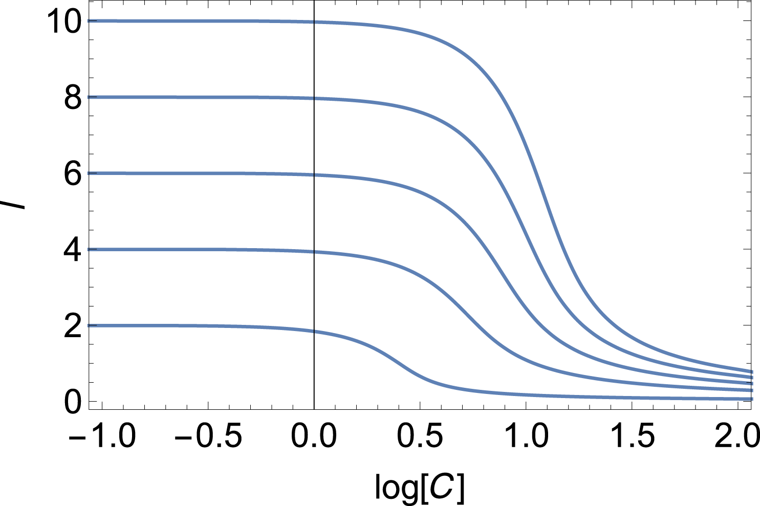
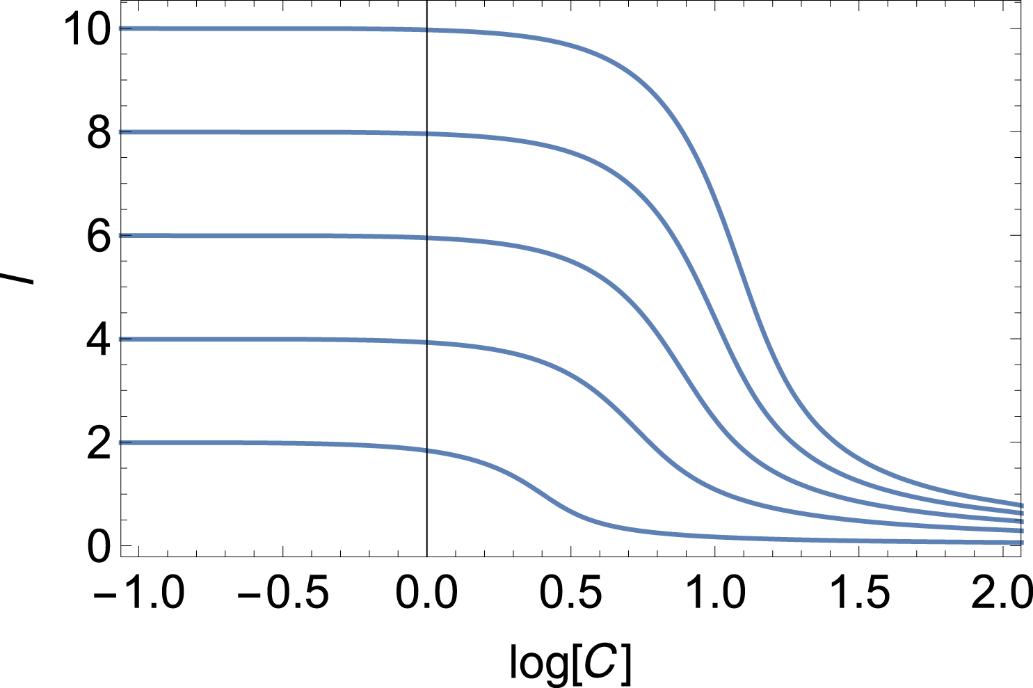
In figure 1 we plot the curves  $l({\mathcal{C}})$ for various
 $2\tilde{m}=2,4,6,8,10$. Each curve starts at a point
 $\{{\mathcal{C}}=0,l=2\tilde{m}\}$. For non-zero current
 ${\mathcal{C}}>0$, the radial dependence becomes more shallow,
 $l<2\tilde{m}$.
Dependence of the radial index  $l$ on the current parameter
 ${\mathcal{C}}$ for various harmonics
 $2\tilde{m}=2,4,6,8,10$.
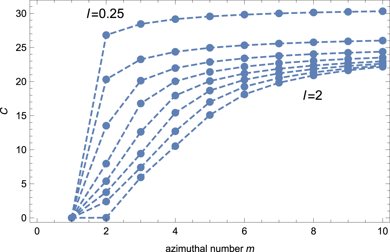
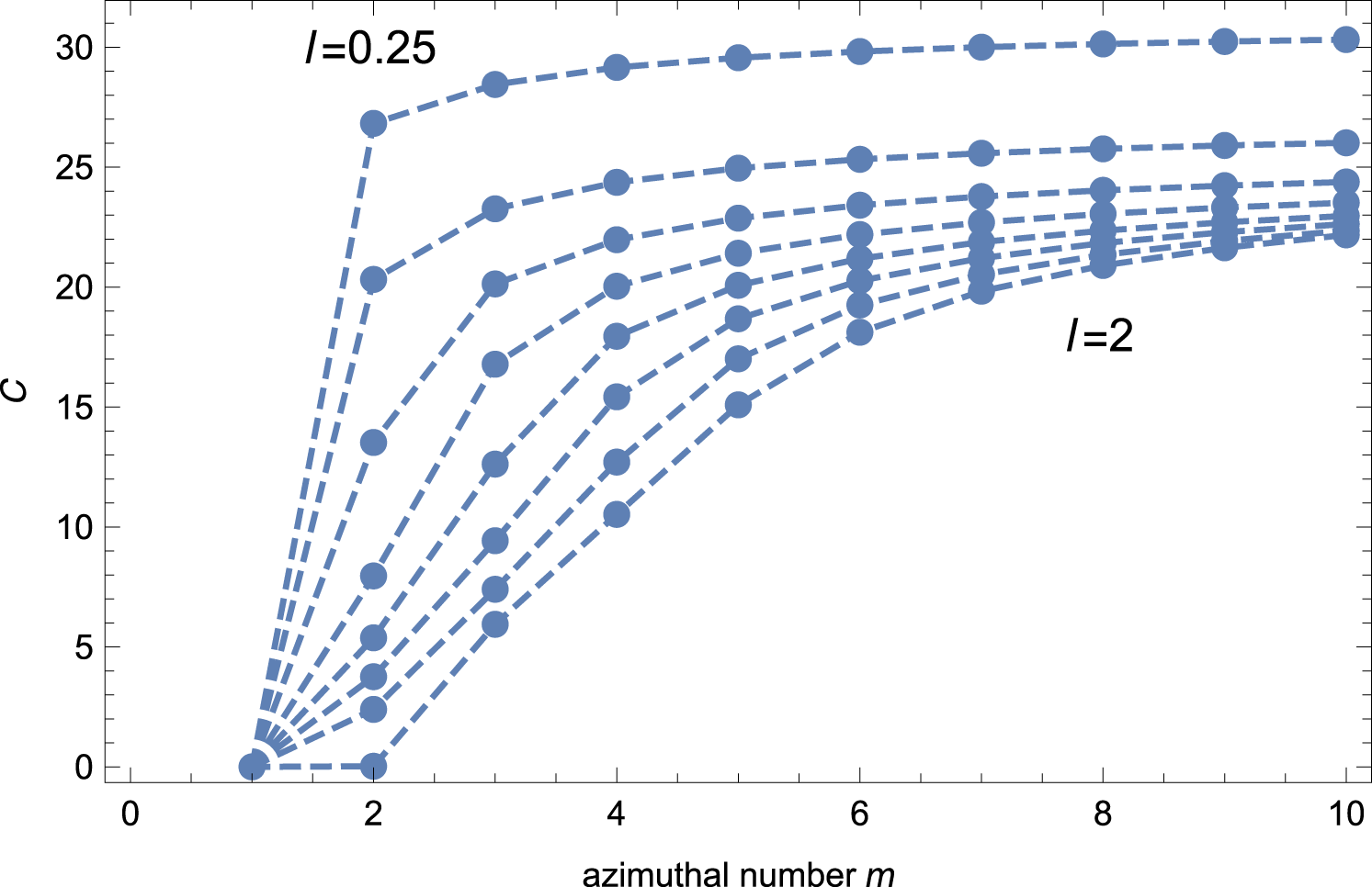
In figure 3 we plot values of  ${\mathcal{C}}$ as a function of azimuthal number
 $m$ for different values of
 $l=0.25,\ldots ,2$. Dashed lines are for convenience only; they connect points corresponding to the same radial parameter
 $l$.
(a) Example of solution  $f(\unicode[STIX]{x1D719})$ for
 $l=1$,
 $2\tilde{m}=2$. In this case
 ${\mathcal{C}}=2.517$. (b) Structure of poloidal field. (Due to the assumed self-similar radial structure, the solutions do not extend to
 $r=0$.) Dashed line is the corresponding vacuum case, equation (2.6).
Values of  ${\mathcal{C}}$ as a function of azimuthal number
 $m$ for different values of
 $l=0.25,\ldots ,2$ (in steps of 0.25). Top curves correspond to smaller
 $l$.
3 Analysis of the solutions
In a formulation of force-free fields in the form
 $$\begin{eqnarray}\displaystyle \text{curl}\,\boldsymbol{B}=\unicode[STIX]{x1D705}\boldsymbol{B}, & & \displaystyle\end{eqnarray}$$
the value of  $\unicode[STIX]{x1D705}$ is
 $$\begin{eqnarray}\displaystyle \unicode[STIX]{x1D705}={\mathcal{C}}\frac{1+l}{lr}f^{1/l}. & & \displaystyle\end{eqnarray}$$
It is constant on flux surfaces  $P$, (2.3).
The current density (we incorporate factors of  $4\unicode[STIX]{x03C0}/c$ into the definition of magnetic field) is
 $$\begin{eqnarray}\displaystyle \left.\begin{array}{@{}c@{}}\displaystyle j_{r}={\mathcal{C}}\frac{1+l}{l}r^{-(l+2)}\unicode[STIX]{x2202}_{\unicode[STIX]{x1D719}}(|f|)^{(1+l)/l},\\ \displaystyle j_{\unicode[STIX]{x1D719}}={\mathcal{C}}(l+1)r^{-(l+2)}(|f|)^{(1+l)/l},\\ \displaystyle j_{z}=r^{-(l+2)}(f^{\prime \prime }+l^{2})=-{\mathcal{C}}^{2}\frac{1+l}{l}r^{-(l+2)}(|f|)^{(2+l)/l}.\end{array}\right\} & & \displaystyle\end{eqnarray}$$
The total axial current is
 $$\begin{eqnarray}\displaystyle I_{z}=\int _{r_{0}}^{\infty }r\,\text{d}r\int _{0}^{2\unicode[STIX]{x03C0}}\text{d}\unicode[STIX]{x1D719}j_{z}=-\frac{r_{0}^{-l}}{l}\int _{0}^{2\unicode[STIX]{x03C0}}\text{d}\unicode[STIX]{x1D719}(f^{\prime \prime }+l^{2}f), & & \displaystyle\end{eqnarray}$$
where  $r_{0}$ is the inner boundary. The total axial current vanishes if the following two conditions are satisfied:
 $$\begin{eqnarray}\displaystyle \left.\begin{array}{@{}c@{}}\displaystyle \int _{0}^{2\unicode[STIX]{x03C0}}f\,\text{d}\unicode[STIX]{x1D719}=0,\\ \displaystyle f^{\prime }(2\unicode[STIX]{x03C0})=f^{\prime }(0).\end{array}\right\} & & \displaystyle\end{eqnarray}$$
All the solutions considered here satisfy these conditions: the second one requires even azimuthal numbers,  $2\tilde{m}$. Generally, there is a larger family of self-similar force-free equilibria with non-zero total axial current.
There is a non-zero toroidal current
 $$\begin{eqnarray}\displaystyle \left.\begin{array}{@{}c@{}}\displaystyle j_{\unicode[STIX]{x1D719}}={\mathcal{C}}(l+1)r^{-2-l}|f|^{(1+l)/l},\\ \displaystyle \int _{0}^{2\unicode[STIX]{x03C0}}\text{d}\unicode[STIX]{x1D719}j_{\unicode[STIX]{x1D719}}\neq 0.\end{array}\right\} & & \displaystyle\end{eqnarray}$$
The radial current density integrated over  $\unicode[STIX]{x1D719}$ satisfies
 $$\begin{eqnarray}\displaystyle j_{r}\propto \int _{0}^{2\unicode[STIX]{x03C0}}\text{d}\unicode[STIX]{x1D719}\unicode[STIX]{x2202}_{\unicode[STIX]{x1D719}}(|f|)^{(1+l)/l}=(|f|)^{(1+l)/l}|_{0}^{2\unicode[STIX]{x03C0}}=0. & & \displaystyle\end{eqnarray}$$
4 Discussion
In this paper we make analytical progress with the highly nonlinear problem(s) of magnetohydrodynamics (Lynden-Bell & Boily Reference Lynden-Bell and Boily1994). We find a class of nonlinear self-similar force-free equilibria in cylindrical geometry. The solutions we find all connect to the vacuum case, in which case the flux function is  $P_{vac}\propto r^{-m}\sin (m\unicode[STIX]{x1D719})$. Structures with vanishing total axial current require even values of
 $m$ (hence
 $m\rightarrow 2\tilde{m}$). For non-zero distributed current with the current parameter
 ${\mathcal{C}}$ the radial dependence changes to
 $r^{-l}$, with
 $l<2\tilde{m}$, while remaining periodic in
 $\unicode[STIX]{x1D719}$ at
 $2\tilde{m}$. Solutions for a given
 $m$ resemble vacuum solutions
 $\propto \sin (2m\unicode[STIX]{x1D719})$, but they are not exactly harmonic in the nonlinear case.
For very large currents the solutions asymptote to  $l\approx 0$, but never reach this limit. The case
 $l=0$ corresponds to
 $B_{r}\propto 1/r$. Mathematically, this is the analogue of the split monopole case in spherical geometry – the split monopole case can be achieved in spherical geometry (with a corresponding anti-monopole in the opposite hemisphere), but is not possible in cylindrical geometry.
Acknowledgements
This work has been supported by NASA grant 80NSSC17K0757 and NSF grants 10001562 and 10001521. I would like to thank J.-J. Aly for comments.