2.1. Model

In this article we consider a two-node tandem network with service rate c₁ at the first node and service rate c₂ < c₁ at the second node; the buffering capacity is infinite at both nodes. Although traffic can enter the first queue in “quanta” of positive size, we assume that it leaves the first queue as “fluid.” In the standard example of packets fed into a communication network, it would mean that during the service of packets in the first queue, the second queue fills at the (net) rate c₁ − c₂.

Let

be the input process; then the amount of traffic generated in the interval (s,t], where s < t and

, is denoted by A(s,t) := A(t) − A(s). We first assume that

has stationary increments; later we focus on the case of stationary independent increments. We denote by Q₁ and Q₂ the steady-state workload at the first and second queue, respectively. Analogously, we denote by Q the total steady-state workload in the tandem network. We assume that

to ensure that both Q₁ and Q₂ are finite a.s.

In this article we focus on the probability that the stationary buffer content at the downstream (i.e., second) node exceeds level u:

Following Reich's representation [30], we can write for the first queue, using the fact that A(·) has stationary increments,

Now note that the following “reduction property” applies, which was also used in [25]. Consider a single queue fed by the original input process

and drained at the slowest of the service rates min{c₁,c₂}. Then it is not hard to see that the buffer content of this queue is equal to the total buffer content of our tandem system (see, e.g., Avi-Itzhak [5] and Friedman [18]). Hence, we have for the total workload Q that

because we assumed that c₂ < c₁.

The above observations directly lead to the following representation for Q₂:

Remark 2.1: It is tempting to explicitly impose the assumption that A(t) is increasing in t, bearing in mind that A(t) is interpreted as the amount of traffic entering the queue in [0,t). However, there are good reasons to not assume a priori that A(·) is increasing, the most prominent being the following.

Consider the superposition of a number of independent and identically distributed (i.i.d.) on-off sources (i.e., sources alternating between sending at some constant, positive rate and being silent); the corresponding input process is evidently increasing. When the number of sources grows large, however, there is, after some appropriate rescaling, convergence to “limit processes” that are not necessarily increasing (for instance, (fractional) Brownian motion (with drift) or Lévy input models; see, e.g., [15,41]). This motivates our choice to not restrict ourselves to increasing inputs.

Two additional comments need to be made. First, we mention that in many cases, the above-mentioned convergence of traffic aggregates carries over to the stationary buffer-content process. Loosely speaking, the queue fed by the aggregate input process converges to the queue fed by the “limit process” (see, e.g., [10,14,15]). Second, notice that when using representation (3), the queue length in the downstream node is necessarily positive.

2.2. A Representation for the Workload Distribution

In this subsection we prove a fundamental result that simplifies the representation (3) for the queue length in the downstream queue Q₂. In particular, we show that the set over which both suprema in (3) should be taken can be decomposed into two adjacent intervals. Define t_u := u/(c₁ − c₂), which can be interpreted as the minimum time it takes for the second queue to exceed level u, starting empty.

Proposition 2.2: Let c₁ > c₂ > 0 and let {X(t),t ≥ 0} be a stochastic process satisfying lim_t→∞{X(t) − c₂ t} = −∞ a.s. Then, for each u ≥ 0,

Proof: We use the short notation Y_S⁽ⁱ⁾ := sup_t∈S{X(t) − c_i t}, for i = 1,2 and

. Define also t_i^{[starf ]} := arg sup_t≥0{X(t) − c_i t}. We have to prove that

Our proof is in four steps.

We now return to the class of arrival processes with stationary increments, that was introduced in Section 2.1. For this class, the above result enables us to rewrite (3) as follows.

Theorem 2.3: For each u ≥ 0,

Proof: The statement follows immediately by combining (3) and Proposition 2.2. █

If the increments of A(·) are also independent, then we get the following representation.

Theorem 2.4: Let

be a stochastic process with stationary independent increments and let

. Then for each u ≥ 0 and A₁(·) and A₂(·) independent copies of the process A(·),

Proof: To get the result, use

Now the theorem follows immediately from the independence and stationarity of the increments of A(·), in conjunction with the fact that (c₁ − c₂)t_u = u. █

3.1. Laplace Transform

In this subsection we assume that

is a spectrally positive Lévy process (see, e.g., [35]) (thus allowing positive jumps). Hence, its Laplace transform is uniquely determined by the Laplace exponent κ(·) through

s ≥ 0; see, for instance, [4, Chap. IX.9].

We need the following additional notation:

where A₁(·) and A₂(·) are independent copies of the process A(·). So we can rewrite formula (4) in Theorem 2.4, with t_u := u/(c₁ − c₂), as

It appears that the function θ₁(·), with

is of crucial importance in the further analysis; observe that θ₁(s) = κ(s) + c₁ s. Additionally, let R_y denote the first-passage time of level y: R_y := inf{t ≥ 0 : −A₂(t) + c₁ t > y}, so that

for each y ≥ 0. We first summarize some useful properties of θ₁(·) and R_y.

Proposition 3.1: Let

be a spectrally positive Lévy process with Laplace exponent κ(·) and

. Then the following hold:

(iii)

for s ≥ 0 and y ≥ 0, where θ₁⁻¹(·) is the inverse function of θ₁(·).

Proof: Part (i) follows from the fact that

, in conjunction with the well-known property that κ(·) is convex. Part (ii) is a consequence of θ₁(s)/s → θ₁′(0+) as s ↓ 0. Part (iii) is an immediate implication of Sato [35, Thm.46.3] (see also, e.g., [8,19]). █

In the following theorem we obtain an explicit formula for the Laplace transform of the downstream queue Q₂.

Theorem 3.2: Let

be a spectrally positive Lévy process with Laplace exponent κ(·) and

. Then, for each x > 0,

Proof: Let x > 0. In the first step, we prove that

Note that integration by parts yields

Moreover, due to (5) and (6) we have

Applying the change of variable v := u/(c₁ − c₂), this leads to

where (9) is due to Proposition 3.1(iii). Now (7) follows directly from combining (8) with (10).

In order to complete the proof, note that, following Zolotarev's result for spectrally positive Lévy processes [42], for x > 0

where

; observe that θ₂(s) = κ(s) + c₂ s = θ₁(s) + (c₂ − c₁)s. Combining (7) with (11) leads to

This completes the proof. █

Remark 3.3: Theorem 3.2 can be considered as an analogue of the result of Zolotarev [42]; there, the Laplace transform of

was given for A(·) being a spectrally positive Lévy process, whereas here we present the corresponding result for

.

Remark 3.4: Recall that Q denotes the (steady state) of the total workload. Since S₁ =_d Q, it follows that (7) is equivalent to

for x ≥ 0. This relation plays a crucial role in Proposition 5.1.

Remark 3.5: We note that for special cases, Theorem 3.2 can be derived in alternative ways. Consider for instance the case of compound Poisson input. We assume that

, where N(·) is a Poisson process with rate λ. The random variables X_i are i.i.d., nonnegative, and independent of N(·). We denote by X the generic random variable and by F(·) its distribution function. Under the above notation, we say that A(·) is a compound Poisson process, characterized by (λ,F). Let

.

Observe that in the tandem setting, the downstream queue is fed by an on–off process: During on-periods, which are distributed as the busy period of the first queue, the downstream queue fills at rate c₁ − c₂, whereas during off-periods, which have an exponential distribution (with mean λ⁻¹), it drains at rate c₂. Assume for ease that μ = λf < 1 = c₂ < 2 = c₁ (the analysis can be extended straightforwardly to the case of general service rates). Under this choice, our formula for

reduces to

Denoting by P the busy period of the first queue, and

and

, then [2, Eq. (3)] gives

It is now left to check that the above two formulas coincide. As the input rate of the first queue equals the output rate of the first queue,

we obtain that

. Hence, it is left to show that

or, equivalently, 2θ₁⁻¹(x) = x + λ − λπ(x) or

By definition, we have θ₁(x) = −λ + λξ(x) + 2x. Also, we have the well-known fixed-point equation for the busy period of the M/G/1 queue (with service rate 2):

Hence, we obtain (13):

as desired. Related results can be found in [24,36].

3.2. Pollaczek–Khintchine Representation

Theorem 3.2 enables us to determine Pollaczek–Khintchine representation for the distribution function of Q₂. Define

and observe that, due to Proposition 3.1,

is a subordinator with

, where ϑ(x) := θ₁⁻¹((c₁ − c₂)x) for y ≥ 0 and x ≥ 0. Recalling Proposition 3.1(ii), we have

with ϱamp; ∈ (0,1).

Thus, following, for example, Takács [38, Eq. (23)], define a distribution function H(·) such that H(x) = 0 for x < 0 and its Laplace transform

is of the form

for x ≥ 0.

Theorem 3.6: Let

be a spectrally positive Lévy process with Laplace exponent κ(·) and

. Then

Proof: Application of Theorem 3.2 immediately yields

This implies Theorem 3.6 immediately. █

Remark 3.7: Theorem 3.6 is related to Theorem 4.1 in [25], where it was assumed that the input process is a compound Poisson.

Remark 3.8: The distribution H(·) has a natural representation in the language of the Lévy measure associated with

. Indeed, since

is a subordinator, then, following [7, Sect. 3.1, Eq. (3)], the Lévy–Khintchine representation of the Laplace exponent ϑ(·) has the following form:

where d is the drift coefficient and Π(s) = Π((s,∞)) is the tail of the Lévy measure. Then

Hence,

for all t ≥ 0. Observe also that

.

4.1. A Dichotomy

If κ(s) exists for negative s, the Lévy process could be called “light-tailed,” as the tail of the distribution of A(1) decays exponentially or faster. In this section we use the results of the previous section to further investigate this light-tailed case, eventually leading to an interesting dichotomy. Throughout this subsection, we tacitly assume that the Lévy input is spectrally positive.

Bearing in mind Proposition 3.1(iii), it is seen that by analytic continuation, Theorem 3.2 holds for all x for which θ₁⁻¹(x(c₁ − c₂)) is well defined. For light-tailed Lévy processes, this means that we could pick any x larger than

(use that θ₁(·) is convex). Theorem 3.2 implies that if, in addition, x > θ₁⁻¹(x(c₁ − c₂)), we have that

is finite and, hence, “Chernoff” implies that

for some finite constant M; see also [1, Lemma3.2]. Let x₂ solve x₂ = θ₁⁻¹(x₂(c₁ − c₂)), or, equivalently, θ₂(x) = 0; if there is no solution, then take the infimum of all x such that θ₂(x) ≤ 0 (this x₂ is necessarily negative). The above arguments immediately lead to the following result, yielding the tightest x for which (15) holds.

Proposition 4.1: If x₂ > arg min_y θ₁(y) then (15) holds (for some M < ∞) for all x > x₁; else (15) holds (for some M < ∞) for all x > x₂.

Assuming that κ(·) is differentiable, define c₁^{[starf ]} := −κ′(x₂); note that x₂ depends on c₂ only (not on c₁) and, consequently, c₁^{[starf ]} depends on c₂ only. The next result indicates that c₁^{[starf ]} can be viewed as a critical service rate, demarcating two regimes.

Proposition 4.2: If c₁ < c₁^{[starf ]}, then (15) holds (for some M < ∞) for all x > x₁; else (15) holds (for some M < ∞) for all x > x₂.

Proof: Due to the convexity of θ₁(·), requiring x₂ > arg inf_y θ₁(y) is equivalent to requiring θ₁′(x₂) > 0. This implies the stated immediately. █

The above indicates that there are in fact two regimes: There is essentially different behaviors for c₁ > c₁^{[starf ]} and c₁ ≤ c₁^{[starf ]}. It is noted that in the first case, the exponential bound (with decay rate x₂) coincides with the traditional Kingman-type bound of a single queue with service rate c₂. We return to this phenomenon later; there we also give an interpretation of the two regimes.

4.2. Tandem with Brownian Motion Input

In this subsection we analyze representation (4) for the case where A(·) = B(·), a standard Brownian motion (with zero drift). It appears that an explicit formula can be derived for

. Let Ψ(·) denote the tail distribution of a standard Normal random variable N:

.

Theorem 4.3: Let A(·) be a standard Brownian motion. Then, for each u ≥ 0,

Proof: Following Theorem 2.4 we have

where B₁(·) and B₂(·) are independent standard Brownian motions. Using the well-known fact that, for each x ≥ 0,

and (see, e.g., Baxter and Donsker [6])

we get two integrals, which we will calculate separately:

where

Integral I₁(u) is evaluated as follows:

For I₂(u), we find

Now integration by parts gives that

, with

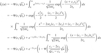
Combining (16) and (17) yields the desired result. █

The next corollary finds the exact asymptotics of the buffer content distribution in the second node, by applying the general result of Theorem 4.3.

Corollary 4.4: Let A(·) be a standard Brownian motion.

Proof: Let J₁(u) and J₂(u) be defined as

and

recall from Theorem 4.3 that

. We also recall the standard “first-order” asymptotic result,

and “second-order” result,

We now consider the three cases separately.

We see that there are two regimes: With c₁^{[starf ]} := 2c₂, there is essentially different behavior for c₁ > c₁^{[starf ]} and c₁ ≤ c₁^{[starf ]}; note that, in the terminology of Section 4.1, we indeed have that c₁^{[starf ]} = −κ′(x₂) (with κ(s) = ½s² and x₂ = −2c₂). In the first case, upon overflow in the second queue, the first queue remains essentially empty and, consequently, the large-buffer asymptotics resemble those of a single queue with service rate c₂. In the second case, the first queue will be exactly “balanced,” as traffic is generated at about a rate of c₁ during t_u units of time.

4.3. Tandem with Poisson Input

Now we assume that A_i(t), with i = 1,2, is Poisson distributed with mean λt (for some λ ∈ (0,c₂)). We first determine

Consider the first of these probabilities. For instance, using the Beneš approach (see, e.g., [31, Eq. (15.1.3)]) with ρ := λ/c₂,

Now consider the second probability. Evidently,

This expression can be computed by conditioning on the value of A₂(t_u), as follows:

Obviously,

Finally, focus on

. Reversing time, it is easily seen that this probability coincides with

Given A₂(t_u) = i, these i arrivals are uniformly distributed on [0,t_u]. Hence, probability (21) equals p(i + x − c₁ t_u,c₁|i,t_u), where p(x,c|N,D) is the overflow probability over level x in a queue with N periodic inputs (with period D) and service rate c (which is sometimes referred to as the N·D/D/1 queue). An explicit expression for p(x,c|N,D) is given in the following lemma.

Lemma 4.5: For x ∈ [0,N] and N < x + c·D, it holds that

with

If N ≥ x + c·D, then p(x,c|N,D) = 0.

Proof: See Humblet, Bhargava, and Hluchyj [21, Sect. III.C], and Roberts and Virtamo [32]. █

This leads to the following expression:

Theorem 4.6: Let A(·) be a Poisson process with rate λ ∈ (0,c₂). Then, for each u ≥ 0,

where ζ(·) and η(·) are given by (20) and (22), respectively.

Remark 4.7: As in Corollary 4.4, one could pursue the exact distribution of Q₂, as in Theorem 4.6, to find its large-buffer asymptotics. However, this turns out to be a nontrivial task, due to the complicated structure of (23).

An alternative is to use a procedure that is similar to the one pursued in [1] for the priority queue. First, realize that the output process of the first queue consists of independent on- and off-periods. The off-periods are obviously exponential (with mean λ⁻¹), whereas the on-periods correspond to the duration of the busy period, say B, in the first queue. The asymptotics of the busy period are known (Cox and Smith [13, Sect.5.6]), and are of the type

for positive numbers α,β, and u → ∞. Standard results for the large-buffer asymptotics of queues fed by a single on–off source now indicate that, as in the Brownian case, there are two regimes, separated by a critical service rate.

The critical service rate can be found as follows. Let θ^{[starf ]} > 0 solve

, or, equivalently, λ(e^θ − 1) = c₂θ, and define λ^{[starf ]} := λe^{θ[starf ]}. If c₁ > c₁^{[starf ]} := λ^{[starf ]}, then the first queue is essentially transparent and the large-buffer asymptotics are purely exponential: α₊ e^−β₊u, with β₊ := θ^{[starf ]}. For c₁ < c₁^{[starf ]}, the large-buffer asymptotics are of the form α₋u^−3/2e^−β₋u; in this case,

We recognize in (24) the Kullback–Leibler distance of a Poisson(c₁) random variable with respect to a Poisson(λ) random variable. Indeed, (24) can be interpreted as the decay rate of the Poisson source generating traffic at rate c₁ during t_u units of time, thus building up an amount of traffic u in the downstream queue.

Remark 4.8: The approach presented in this subsection is not restricted to the Poisson input of batches of deterministic (unit) size. Let us, for instance, consider the situation of a Poisson(λ) stream of nonnegative i.i.d. batches

. It turns out that Theorem 1 of Takács [39, p.24] is quite useful here. To make this theorem directly applicable, assume for the moment that time is slotted (i.e., the number of batches arriving per slot has a Poisson distribution with mean λ), c₁ = 1, and that the batch sizes are i.i.d. and take on nonnegative integral values.

We can repeat the above argument. Now ζ(·) is the overflow probability in the corresponding M/G/1 queue, which is explicitly given by the Pollaczek–Khintchine formula; see, for instance, [4, Thm. 5.7, Eq. (5.5)]. Also, η(·) follows easily: We can use exactly the same procedure as earlier, by first conditioning on the value of A₂(t_u); note that the per-slot arrivals are interchangeable random variables, such that the counterpart of probability (21) follows immediately from [39, Thm.1, p.24].

5.1. Tandem with α-Stable Lévy Input

In this subsection we focus on the case of α-stable Lévy input. Let X_α,σ,β(·) denote an α-stable Lévy motion with scale parameter σ and skewness parameter β (see, e.g., [34]). We analyze

for A(·) an α-stable Lévy motion with α ∈ (1,2), σ = 1, and β ∈ (−1,1]. For the general case of β ∈ (−1,1], we present the generic asymptotic upper and lower bounds for

in the large-buffer regime (i.e., u → ∞). Moreover, if β = 1, then the application of Proposition 5.1 provides us with the exact asymptotics of

.

In the rest of this section we use the notation

Theorem 5.3: Let A(t) = X_α,1,β(t) with α ∈ (1,2) and β ∈ (−1,1]. Then the following hold:

The following lemma from [29] (see also [20, Prop. 3.7], where the substitution β := −β matches our notation) is needed in our analysis.

Lemma 5.4: Let α ∈ (1,2), β ∈ (−1,1], and c > 0. Then

as u → ∞.

Proof of Theorem 5.3: Let X_α,1,β(·) and Y_α,1,β(·) be mutually independent α-stable Lévy motions and recall that, as earlier, t_u = u/(c₁ − c₂).

In the following theorem we analyze an important special case of the α-stable Lévy input process where β = 1. The importance of this class of input processes stems, for example, from [27,41], where it was proved that X_α,1,1(·) (α ∈ (1,2)) can be used as an approximation for an appropriately scaled superposition of many on–off input processes.

Theorem 5.5: Let A(·) = X_α,1,1(·) with α ∈ (1,2). Then, as u → ∞,

Proof: The combination of Proposition 5.1 with Lemma 5.4 gives

Routine calculation, as in [20, Chap.3], yields that

which completes the proof. █

Remark 5.6: Observe that the exact asymptotic presented in Theorem 5.5 matches the lower bound given in Theorem 5.3. We conjecture that this observation extends to the whole range of parameters β ∈ (−1,1].

5.2. Tandem with Compound Poisson Input, with Regularly Varying Jumps

Consider again the case of compound Poisson(λ,F) input. In the following theorem, we present the exact asymptotics of the tail distribution of Q₂ under the assumption that F(·) is regularly varying at ∞.

Theorem 5.7: Let A(·) correspond to a compound Poisson process (λ,F). Suppose that

where α ∈ (1,2), [ell ](·) is slowly varying at ∞, and

. Then

as u → ∞.

Proof: Observe that

. Following [3, Thm.2.1], we have that

as u → ∞. Thus, using Karamata's theorem, we have

as u → ∞. Hence, the theorem follows by application of Proposition 5.1. █