2.1. Characterization of rate function

For practical applications, we need to further study the rate function $I(\cdot)$ defined by (3). In this subsection, some properties and characterization of I will be established.

Set $\textrm{Dom}(I)=\left\{f: I(f)<+\infty\right\}$ and define the following mapping $\mathbb S$ on $L^{2}([0,1])$ :

(4) \begin{equation} \mathbb S(\phi)(t)=\int^{1}_{0}K(t,r)\phi(r) \, \textrm{d} r, \qquad \phi\in L^{2}([0,1]), \quad t\in[0,1].\end{equation}

Obviously, $\mathbb S(L^{2}([0,1]))\,:\!=\,\left\{\mathbb S(\phi): \phi\in L^{2}([0,1])\right\}$ is the reproducing kernel Hilbert space associated with Gaussian process Y defined by (1).

Proof. By the definition of $I(\cdot)$ in (3), (i) is obvious. Then, we turn to prove (ii). In fact, for any $f\in \textrm{Dom}(I)$ , there exists a sequence of $\phi_{n}\in L^{2}([0,1])$ such that

\begin{equation*}f(t)=\int^{1}_{0}K(t,r)\phi_{n}(r) \, \textrm{d} r, t\in[0,1], \quad \text{and} \quad \lim\limits_{n\to+\infty}\frac{1}{2}\int^{1}_{0}\phi^{2}_{n}(r) \, \textrm{d} r=I(f).\end{equation*}

Then, there exists a subsequence of $\phi_{n_i}$ converging weakly to an element $\phi\in L^{2}([0,1])$ , which implies that

\begin{equation*}f(t)=\int^{1}_{0}K(t,r)\phi(r) \, \textrm{d} r, \qquad t\in[0,1].\end{equation*}

Note that for any $\psi\in L^{2}([0,1])$ ,

\begin{align*}\left|\int^{1}_{0}\phi(r)\psi(r) \, \textrm{d} r\right|&=\lim_{n_i\to\infty}\left|\int^{1}_{0}\phi_{n_i}(r)\psi(r) \, \textrm{d} r\right|\\&\leq\left(\int^{1}_{0}\psi^{2}(r) \, \textrm{d} r\right)^{1/2}\left(\lim\limits_{n_i\to+\infty}\int^{1}_{0}\phi^{2}_{n_i}(r) \, \textrm{d} r\right)^{1/2},\end{align*}

which implies that

\begin{equation*}\frac{1}{2}\int^{1}_{0}\phi^{2}(r) \, \textrm{d} r\leq \frac{1}{2}\lim\limits_{n_i\to+\infty}\int^{1}_{0}\phi^{2}_{n_i}(r) \, \textrm{d} r = I(f).\end{equation*}

Moreover, by the definition of I(f), we also have

\begin{equation*}\frac{1}{2}\int^{1}_{0}\phi^{2}(r) \, \textrm{d} r \geq I(f).\end{equation*}

Therefore, $I(f)=\frac{1}{2}\int^{1}_{0}\phi^{2}(r) \, \textrm{d} r$ .

Finally, we show the uniqueness of $\phi$ . Suppose there exists some $\psi\in L^{2}([0,1])$ such that the infimum is obtained, and $\psi\neq\phi$ in $L^{2}([0,1])$ . Then there exists a measurable set $A\subset [0,1]$ such that, for any $r\in A$ , $\psi(r)\neq\phi(r)$ and $\mathcal{L}(A)\neq0$ . Define 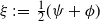$\xi\,:\!=\,\frac{1}{2}(\psi+\phi)$ ; then,

\begin{equation*}f(t)=\int^{1}_{0}K(t,r)\xi(r) \, \textrm{d} r \quad \text{and} \quad \int^{1}_{0}\xi^{2}(r) \, \textrm{d} r = \int_{A}\xi^{2}(r) \, \textrm{d} r + \int_{A^{c}}\xi^{2}(r) \, \textrm{d} r.\end{equation*}

By the strict convexity of $x^{2}$ ,

\begin{align*} \int_{A}\xi^{2}(r) \, \textrm{d} r & < \frac{1}{2}\left(\int_{A}\phi^{2}(r) \, \textrm{d} r+\int_{A}\psi^{2}(r) \, \textrm{d} r\right), \\[4pt] \int_{A^c}\xi^{2}(r) \, \textrm{d} r & \leq \frac{1}{2}\left(\int_{A^c}\phi^{2}(r) \, \textrm{d} r+\int_{A^c}\psi^{2}(r) \, \textrm{d} r\right).\end{align*}

Therefore, $\frac{1}{2}\int^{1}_{0}\xi^{2}(r) \, \textrm{d} r < I(f)$ , which contradicts the definition of I(f).

Now, we give an equivalent expression of the rate function $I(\cdot)$ .

Proposition 2.2. Assume that $\mathbb S$ is an injection on $L^{2}([0,1])$ . Under Conditions 1.1 and 1.2, we have

\begin{equation*}I(f)=\left\{\begin{array}{ll} \frac{1}{2}\left\|\mathbb S^{-1}f\right\|^{2}_{L^{2}([0,1])}, & \textrm{if } f\in\mathbb S(L^{2}([0,1])) , \\[8pt] +\infty,& \textrm{otherwise}.\\\end{array}\right.\end{equation*}

I is also the rate function of the probability measures $\left\{\mu_{\epsilon}, \epsilon>0\right\}$ on C ([0, 1]) with speed $\epsilon$ , where

\begin{equation*}\mu_{\epsilon}(A)\,:\!=\,\mathbb{P}\left(\sqrt{\epsilon}\int^{1}_{0}K(\cdot,r) \, \textrm{d} W(r)\in A\right),\qquad A\subseteq C([0,1]),\end{equation*}

and $\left\{W(r): r\in[0,1]\right\}$ is a Brownian motion in the probability space $\left(\Omega, \mathcal F, \mathbb{P}\right)$ .

Proof. By the definition of I and $\mathbb S$ , the first result is easily obtained if $\mathbb S$ is an injection.

Now we turn to the second result. For any finite sign measure $\nu$ on [0, 1], by stochastic Fubini’s theorem [Reference Zabczyk and Da Prato20, Theorem 4.18] we have

\begin{equation*}\int^{1}_{0}\int^{1}_{0}K(t,r) \, \textrm{d} W(r)\nu(\textrm{d} t) = \int^{1}_{0}\int^{1}_{0}K(t,r)\nu(\textrm{d} t) \, \textrm{d} W(r),\end{equation*}

which implies that $\int^{1}_{0}\int^{1}_{0}K(t,r) \, \textrm{d} W(r)\nu(\textrm{d} t)\sim N\big(0, \int^{1}_{0}\big(\int^{1}_{0}K(t,r)\nu(\textrm{d} t)\big)^{2} \, \textrm{d} r\big)$ . By [Reference Deuschel and Stroock11, Theorem 3.4.12] with the Cameron–Martin space $H=\{h; h=\int^{t}_{0}\dot{h}(r) \, \textrm{d} r; \dot{h}\in L^{2}([0,1])\}$ , $E=C([0,1])$ , and $S: H\to E$ defined by $S(h)=\int^{1}_{0} K(t,r)\dot{h}(r) \, \textrm{d} r$ , it is sufficient to prove that

\begin{equation*}S^{*}(\nu)(r)=\int^{r}_{0}\int^{1}_{0}K(t,r)\nu(\textrm{d} t) \, \textrm{d} r, \qquad r\in[0,1]\end{equation*}

in H, where $S^{*}$ is the adjoint map to S.

Indeed, by the definition of S, we have, for any $h\in H$ ,

\begin{equation*}\langle S^{*}(\nu), h\rangle = \langle \nu, S(h)\rangle = \int^{1}_{0}\!\!\left(\int^{1}_{0}\!\! K(t,r)\dot{h}(r) \, \textrm{d} r\right)\!\nu(\textrm{d} t)=\int^{1}_{0}\!\!\left(\int^{1}_{0}\!\! K(t,r)\nu(\textrm{d} t)\right)\!\dot{h}(r) \, \textrm{d} r.\end{equation*}

Therefore, $S^{*}(\nu)(r)=\int^{r}_{0}\int^{1}_{0}K(t,r)\nu(\textrm{d} t) \, \textrm{d} r$ for $r\in[0,1]$ , and the desired result is proved.

Note that the operator $\mathbb{S}$ may not be injective, or not easy to verify. However, when the kernel K has some product structure, the rate function has the following explicit formulation.

Proposition 2.3. Suppose that $K(t,r)=\xi(t)\eta(r)\mathbf{1}_{[0,t]}(r)$ , $t,r\in[0,1]$ . Here, $\xi$ and $\eta$ are measurable functions satisfying $\xi\in C([0,1])$ , $\eta\in L^{2}([0,1])$ , and $\mathcal{L}(\{\xi=0\})=0$ . Under Conditions 1.1 and 1.2, we have

\begin{equation*} \begin{aligned} I(f)=\left\{ \begin{array}{l@{\quad}l} \frac{1}{2}\int^{1}_{0}\big(\big(\frac{f}{\xi}\big)'(r)\big)^{2}\frac{\mathbf{1}_{\{\eta\neq0\}}(r)}{\eta^{2}(r)} \textrm{d} r, & if\ \frac{f}{\xi}\textit{is absolutely continuous and} \\[8pt] & \big(\frac{f}{\xi}\big)'\frac{\mathbf{1}_{\{\eta\neq0\}}}{\eta}\in L^2([0,1]) , \\[8pt] +\infty, & \textit{otherwise}. \end{array}\right. \end{aligned}\end{equation*}

Proof. If $f\in \textrm{Dom}(I)$ then, for any choice $\phi\in L^{2}([0,1])$ such that

\begin{equation*}f(t)=\xi(t)\int^{t}_{0}\eta(r)\phi(r) \, \textrm{d} r, \qquad t\in[0,1],\end{equation*}

the fact that $\mathcal{L}(\{\xi=0\})=0$ implies that $\frac{f}{\xi}(t)=\int^{t}_{0}\eta(r)\phi(r) \, \textrm{d} r$ is absolutely continuous and, for almost all $t\in[0,1]$ , 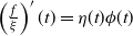$\left(\frac{f}{\xi}\right)'(t)=\eta(t)\phi(t)$ . That is, on $\{t: \eta(t)\neq0\}$ , 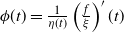$\phi(t)=\frac{1}{\eta(t)}\left(\frac{f}{\xi}\right)'(t)$ .

Define 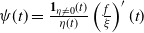$\psi(t)=\frac{\mathbf{1}_{\eta\neq0}(t)}{\eta(t)}\left(\frac{f}{\xi}\right)'(t)$ for almost all $t\in[0,1]$ . Then $\psi(t)=\phi(t)\mathbf{1}_{\{\eta\neq0\}}(t)$ for almost all $t\in[0,1]$ , and

\begin{equation*}f(t)=\xi(t)\int^{t}_{0}\eta(r)\psi(r) \, \textrm{d} r, \qquad t\in[0,1].\end{equation*}

Obviously, $\int^{1}_{0}\phi^{2}(r) \, \textrm{d} r\geq \int^{1}_{0} \phi^{2}(r)\mathbf{1}_{\{\eta(r)\neq0\}} \, \textrm{d} r = \int^{1}_{0}\psi^{2}(r) \, \textrm{d} r$ , which completes the proof of this proposition.

2.2. Applications

In this subsection we apply our results in Theorem 1.1 and Propositions 2.2 and 2.3 to the weak approximation of some Gaussian processes.

2.2.1 Moving average of Brownian motion

Let the kernel $K(t,r)=\mathbf{1}_{[0,t]}(r)(2\pi)^{1/2}(t-r)^{H-1/2}$ , with $0<H<1/2$ . It is well known that the corresponding mapping $\mathbb S$ defined by (4) is an injection and $\mathbb S^{-1}f$ is known as the solution to Abel’s equation [Reference Samko, Kilbas and Marichev17, (2.1), p. 29]. By [Reference Samko, Kilbas and Marichev17, Theorem 2.1], $f\in\mathbb S(L^{2}([0,1]))$ implies that 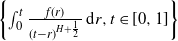$\left\{\int^{t}_{0}\frac{f(r)}{(t-r)^{H+\frac{1}{2}}} \, \textrm{d} r, t\in[0,1]\right\}$ is absolutely continuous, 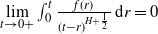$\lim\limits_{t\to0+}\int^{t}_{0}\frac{f(r)}{(t-r)^{H+\frac{1}{2}}} \, \textrm{d} r=0$ . Furthermore, if $f\in\mathbb S(L^{2}([0,1]))$ , then $f(t)=\int_0^1K(t,r)\phi(r) \, \textrm{d} r$ , where $\phi\in L^{2}([0,1])$ [Reference Samko, Kilbas and Marichev17, (2.6), p. 30] can be written as

(5) \begin{equation}\phi(t)=-\frac{1}{\sqrt{2\pi}\Gamma\big(\frac{1}{2}+H\big)\Gamma\big(\frac{1}{2}-H\big)}\frac{\textrm{d}}{\textrm{d} t}\left(\int^{1}_{t}\frac{f(r) \, \textrm{d} r}{(t-r)^{H+\frac{1}{2}}}\right).\end{equation}

It is also known that Conditions 1.1 and 1.2 both hold with $G(t)=Ct$ , $C>0$ , $\alpha=2H$ [Reference Delgado and Jolis9].

Now, let $Y_{\epsilon}(t)=\frac{(2\pi)^{1/2}}{\epsilon}\int^{t}_{0}(t-r)^{H-1/2}(-1)^{N(\epsilon^{-2}r)} \, \textrm{d} r$ , $0\leq t\leq1$ . By using Theorem 1.1 and Proposition 2.2, we have the following result.

Corollary 2.1. The family $\left\{\lambda_{\epsilon}Y_{\epsilon},\epsilon>0\right\}$ satisfies the sample path moderate deviation with speed $\lambda^{2}_{\epsilon}$ and rate function I defined by

$$I(f) = \left\{ {\begin{array}{*{20}{c}} {\frac{1}{2}\int_0^1 {{\phi ^2}} (r){\mkern 1mu} {\rm{d}}r,} & {if\int_0^t {\frac{{f(r)}}{{{{(t - r)}^{H + \frac{1}{2}}}}}} {\mkern 1mu} {\rm{d}}r\;is\ absolutely\ continuous\ and} \\[12pt] & {\mathop {\lim }\limits_{t \to 0 + } \int_0^t {\frac{{f(r)}}{{{{(t - r)}^{H + \frac{1}{2}}}}}} {\mkern 1mu} {\rm{d}}r = 0,} \\[10pt] { + \infty ,} & {otherwise.} \\ \end{array}} \right.{\rm{ }}$$

Here, $\phi\in L^{2}([0,1])$ is given by (5).

2.2.2. Fractional Brownian motion

For $K^{H}(t,r)$ given by (2), $Y(t)\,:\!=\,\int_0^1K^{H}(t,r) \, \textrm{d} W(r)$ is a fractional Brownian motion with Hurst index H. Applying [Reference Decreusefond and Üstünel8, Theorem 2.1], the mapping $\mathbb S$ defined by (4) is an injection. Moreover, Conditions 1.1 and 1.2 both hold with $G(t)=Ct$ , $C>0$ , $\alpha=2H$ [Reference Delgado and Jolis9].

Let $Y_{\epsilon}(t)=\frac{1}{\epsilon}\int^{1}_{0}K^{H}(t,r)(-1)^{N(\epsilon^{-2}r)} \, \textrm{d} r$ , $0\leq t\leq1$ . Together with Theorem 1.1 and Corollary 2.2, the following result holds.

Corollary 2.2. The family $\left\{\lambda_{\epsilon}Y_{\epsilon},\epsilon>0\right\}$ satisfies the sample path moderate deviation with speed $\lambda^{2}_{\epsilon}$ and rate function I given by

\begin{equation*}I(f)=\left\{\begin{array}{ll}\frac{1}{2}\left\|\mathbb S^{-1}f\right\|^{2}_{L^{2}([0,1])}, & \textit{if}\ f\in\mathbb S(L^{2}([0,1])) , \\[5pt] +\infty,& \textit{otherwise}.\\\end{array}\right.\end{equation*}

2.2.3. Ornstein–Uhlenbeck process

For the kernel $K(t,r)=C\textrm{e}^{\lambda(r-t)}\mathbf{1}_{(0,t]}(r)$ with $\lambda>0$ , Conditions 1.1 and 1.2 both hold with $G(t)=Ct$ , $C>0$ [Reference Delgado and Jolis9]. In particular, $Y_t\,:\!=\,\int_0^1C\textrm{e}^{\lambda(r-t)} \, \textrm{d} W(r)$ satisfies $\textrm{d} Y_t=-\lambda Y_t+C \, \textrm{d} W(t)$ . Hence, this process is the well-known Ornstein–Uhlenbeck process.

Let $Y_{\epsilon}(t)=\frac{1}{\epsilon}\int^{t}_{0}C\textrm{e}^{\lambda(r-t)}(-1)^{N(\epsilon^{-2}r)} \, \textrm{d} r$ , $0\leq t\leq1$ . By Theorem 1.1 and Corollary 2.3, we conclude this section with the following corollary.

Corollary 2.3. $\{\lambda_{\epsilon}Y_{\epsilon},\epsilon>0\}$ satisfies the sample path moderate deviation with speed $\lambda^{2}_{\epsilon}$ and rate function I defined by

\begin{equation*} \begin{aligned} I(f)=\left\{ \begin{array}{l@{\quad}l} \frac{1}{2C^{2}}\int^{1}_{0}(f'(r)+\lambda f(r))^{2} \textrm{d} r, & \textit{if }\ f\ \textit{is absolutely continuous and} \\[4pt] & \int^{1}_{0}|f'(r)|^{2} \textrm{d} r<+\infty , \\[4pt] +\infty, & \textit{otherwise}. \\ \end{array}\right. \end{aligned}\end{equation*}

3.1. High-order moments

For any $f\in L^{2}([0,1])$ , we extend the result in [Reference Delgado and Jolis9, Lemma 2], and then give a sharper estimation for the high-order moments of $\int^{1}_{0}f(r)\theta_{\epsilon}(r) \, \textrm{d} r$ .

Lemma 3.1. For any $f\in L^{2}([0,1])$ and even number $m\in\mathbb N$ ,

\begin{equation*} \begin{aligned} \left(\mathbb E\left(\int^{1}_{0}f(r)\theta_{\epsilon}(r) \, \textrm{d} r\right)^{m}\right)^{1/m}\leq \textrm{e}^{-\frac{1}{2}}\left(\frac{\textrm{e}}{\sqrt{\pi}\,}\right)^{\frac{1}{m}}\sqrt{m}\left(\int_0^1f^{2}(r) \, \textrm{d} r\right)^{1/2}. \end{aligned}\end{equation*}

Proof. We have

\begin{align*} &\mathbb E\left(\int^{1}_{0}f(r)\theta_{\epsilon}(r) \, \textrm{d} r\right)^{m}\\ & =\frac{m!}{\epsilon^{m}}\int_{[0,1]^{m}}\mathbf{1}_{\{r_{1}<\cdots<r_{m}\}}f(r_{1})\cdots f(r_{m})\exp\left\{-\frac{2}{\epsilon^{2}}\sum^{m/2}_{i=1}(r_{2i}-r_{2i-1}) \right\} \, \textrm{d} r_{1}\cdots \textrm{d} r_{m} \\ &=\frac{m!}{\epsilon^{m-2}}\int_{[0,1]^{m-2}}\mathbf{1}_{\{r_{3}<\cdots<r_{m}\}}G_{1}(r_{3})f(r_{3})\cdots f(r_{m}) \times \exp\left\{-\frac{2}{\epsilon^{2}}\sum^{m/2}_{i=3}(r_{2i}-r_{2i-1}) \right\} \, \textrm{d} r_{3}\cdots \textrm{d} r_{m},\end{align*}

where the first equality is shown in [Reference Delgado and Jolis9, Lemma 2] and, for any $r_{3}<r_{4}$ ,

\begin{align*}G_{1}(r_{3})\,:\!= &\int_{[0,1]^{2}}\mathbf{1}_{\{r_{1}<r_{2}<r_{3}\}}\frac{f(r_{1})}{\epsilon}\cdot\frac{f(r_{2})}{\epsilon}\exp\left\{-\frac{2}{\epsilon^{2}}(r_{2}-r_{1})\right\} \, \textrm{d} r_{1} \, \textrm{d} r_{2} \\[3pt] & \leq \left(\int_{[0,1]^{2}}\mathbf{1}_{\{r_{1}<r_{2}<r_{3}\}}\frac{f^{2}(r_{1})}{\epsilon^{2}}\exp\left\{-\frac{2}{\epsilon^{2}}(r_{2}-r_{1})\right\} \, \textrm{d} r_{1} \, \textrm{d} r_{2}\right)^{1/2} \\[3pt] & \times \left(\int_{[0,1]^{2}}\mathbf{1}_{\{r_{1}<r_{2}<r_{3}\}}\frac{f^{2}(r_{2})}{\epsilon^{2}}\exp\left\{-\frac{2}{\epsilon^{2}}(r_{2}-r_{1})\right\} \, \textrm{d} r_{1} \, \textrm{d} r_{2}\right)^{1/2} \\[3pt] &\leq\frac{1}{2}\left(\int_{r_{1}<r_{3}}f^{2}(r_{1}) \, \textrm{d} r_{1}\right)^{1/2} \cdot\left(\int_{r_{2}<r_{3}}f^{2}(r_{2}) \, \textrm{d} r_{2}\right)^{1/2} \\[3pt] &\leq\frac{1}{2}\left(\int_{r<r_{3}}f^{2}(r) \, \textrm{d} r\right)^{1/2} \cdot\left(\int_{r<r_{4}}f^{2}(r) \, \textrm{d} r\right)^{1/2}.\end{align*}

Substituting the above estimation into the original equation,

\begin{align*}\mathbb E\left(\int^{1}_{0}f(r)\theta_{\epsilon}(r) \, \textrm{d} r\right)^{m} = & \frac{m!}{\epsilon^{m-4}}\int_{[0,1]^{m-4}}\mathbf{1}_{\{r_{5}<\cdots<r_{m}\}}G_{2}(r_{5})f(r_{5})\cdots f(r_{m}) \\[4pt] & \times\exp\left\{-\frac{2}{\epsilon^{2}}\sum^{m/2}_{i=5}(r_{2i}-r_{2i-1}) \right\} \, \textrm{d} r_{5}\cdots \textrm{d} r_{m},\end{align*}

where, for any $r_{5}<r_{6}$ ,

\begin{align*}G_{2}(r_{5}) \,:\!= & \int_{[0,1]^{2}}\mathbf{1}_{\{r_{3}<r_{4}<r_{5}\}}G_{1}(r_{3})\frac{f(r_{3})}{\epsilon}\cdot\frac{f(r_{4})}{\epsilon}\exp\left\{-\frac{2}{\epsilon^{2}}(r_{4}-r_{3})\right\} \, \textrm{d} r_{3} \, \textrm{d} r_{4} \\[4pt] &\leq\frac{1}{2}\int_{[0,1]^{2}}\mathbf{1}_{\{r_{3}<r_{4}<r_{5}\}}\left(\int_{r<r_{3}}f^{2}(r) \, \textrm{d} r\right)^{1/2}\frac{f(r_{3})}{\epsilon}\exp\left\{-\frac{1}{\epsilon^{2}}(r_{4}-r_{3})\right\} \\[4pt] & \times \left(\int_{r<r_{4}}f^{2}(r) \, \textrm{d} r\right)^{1/2}\frac{f(r_{4})}{\epsilon}\exp\left\{-\frac{1}{\epsilon^{2}}(r_{4}-r_{3})\right\} \, \textrm{d} r_{3} \, \textrm{d} r_{4}\end{align*}

$$\matrix{ { \le {1 \over {{2^2}}}{{\left( {\int_{{r_3} < {r_5}} {\left( {\int_{r < {r_3}} {{f^2}} (r){\mkern 1mu} {\rm{d}}r} \right)} {f^2}({r_3}){\mkern 1mu} {\rm{d}}{r_3}} \right)}^{1/2}}} \hfill \cr { \times {{\left( {\int_{{r_4} < {r_5}} {\left( {\int_{r < {r_4}} {{f^2}} (r){\mkern 1mu} {\rm{d}}r} \right)} {f^2}({r_4}){\mkern 1mu} {\rm{d}}{r_4}} \right)}^{1/2}}} \hfill \cr { \le {1 \over {{2^2}}}{{\left( {{{{{\left( {\int_{r < {r_5}} {{f^2}} (r){\mkern 1mu} {\rm{d}}r} \right)}^2}} \over 2}} \right)}^{1/2}}{{\left( {{{{{\left( {\int_{r < {r_6}} {{f^2}} (r){\mkern 1mu} {\rm{d}}r} \right)}^2}} \over 2}} \right)}^{1/2}}.} \hfill \cr } $$

Substituting the above into the previous equation again, by the same argument and induction, we have

\begin{equation*}\mathbb E\left(\int^{1}_{0}f(r)\theta_{\epsilon}(r) \, \textrm{d} r\right)^{m}\leq\frac{m!}{2^{m/2}}\cdot\frac{\big(\int_0^1f^{2}(r) \, \textrm{d} r\big)^{m/2}}{(m/2)!}.\end{equation*}

For any positive integer n, we have the following Stirling formula:

(6) \begin{equation}\sqrt{2\pi n}\left(\frac{n}{\textrm{e}}\right)^{n}\leq n!\leq \textrm{e}\sqrt{n}\left(\frac{n}{\textrm{e}}\right)^{n}.\end{equation}

Therefore, $\frac{m!}{(m/2)!}\leq \frac{\textrm{e}}{\sqrt{\pi}\,}\cdot 2^{\frac{m}{2}} \cdot\exp\big\{\frac{m\log m}{2}-\frac{m}{2}\big\}$ . Then,

(7) \begin{equation}\mathbb E\left(\int^{1}_{0}f(r)\theta_{\epsilon}(r) \, \textrm{d} r\right)^{m}\leq \frac{\textrm{e}}{\sqrt{\pi}\,}\exp\left\{\frac{m}{2}\log m-\frac{m}{2}\right\}\left(\int_0^1f^{2}(r) \, \textrm{d} r\right)^{m/2}.\end{equation}

Therefore, $\left(\mathbb E\left(\int^{1}_{0}f(r)\theta_{\epsilon}(r) \, \textrm{d} r\right)^{m}\right)^{1/m}\leq \textrm{e}^{-\frac{1}{2}}\left(\frac{\textrm{e}}{\sqrt{\pi}\,}\right)^{\frac{1}{m}}\sqrt{m}\left(\int_0^1f^{2}(r) \, \textrm{d} r\right)^{1/2}$ .

As an application of Lemma 3.1 we can obtain the following result, which plays a crucial role in our analysis.

Corollary 3.1. For any $0\leq\eta<\frac{1}{2}$ ,

\begin{equation*}\sup_{f\in L^{2}([0,1]),\|f\|_{L^{2}}\neq0}\mathbb E\exp\left\{\frac{\eta\big|\int^{1}_{0}f(r)\theta_{\epsilon}(r) \, \textrm{d} r\big|^2}{\int_0^1f^2(r) \, \textrm{d} r}\right\}<\infty.\end{equation*}

Proof. Using (7) and the Stirling formula (6), for any $0\leq\eta<\frac{1}{2}$ ,

\begin{align*}\mathbb E\exp\left\{\frac{\eta\big|\int^{1}_{0}f(r)\theta_{\epsilon}(r) \, \textrm{d} r\big|^{2}}{\int_0^1f^2(r) \, \textrm{d} r}\right\}&=\sum_{n=0}^{\infty}\frac{1}{n!}\frac{\eta^n\mathbb E\big|\int^{1}_{0}f(r)\theta_{\epsilon}(r) \, \textrm{d} r\big|^{2n}}{\left(\int_0^1f^2(r) \, \textrm{d} r\right)^n} \\&\leq \frac{\textrm{e}}{\sqrt{\pi}\,}\left(1+\sum_{n=1}^{\infty}\frac{(2\eta)^n}{\sqrt{2\pi n}\,}\right)<+\infty,\end{align*}

which completes the proof of this corollary.

3.2. Finite-dimensional moderate deviations

In this subsection, for fixed $0<t_1<\cdots<t_k\leq1$ , we will study the moderate deviations for $\lambda_{\epsilon}\big(Y_{\epsilon}(t_1),\cdots,Y_{\epsilon}(t_k)\big)^{\top}$ . Since $K(t_i,\cdot)\in L^{2}([0,1])$ , there exists a sequence of finite variational functions (step functions, for example) $\left\{K_{m}(t,\cdot), m\in\mathbb N\right\}$ such that

\begin{equation*}\lim_{m\to\infty}\max_{1\leq i\leq k}\int_0^1\big|K(t_i,r)-K_{m}(t_i,r)\big|^2 \, \textrm{d} r=0.\end{equation*}

Define

\begin{align*} Y_{\epsilon}(t_1,\ldots, t_k) & = \left(\int^{1}_{0}K(t_1,r)\theta_{\epsilon}(r) \, \textrm{d} r,\ldots, \int^{1}_{0}K(t_k,r)\theta_{\epsilon}(r) \, \textrm{d} r\right)^{\top} , \\Y_{m,\epsilon}(t_1,\ldots, t_k) & = \left(\int^{1}_{0}K_{m}(t_1,r)\theta_{\epsilon}(r) \, \textrm{d} r,\ldots, \int^{1}_{0}K_{m}(t_k,r)\theta_{\epsilon}(r) \, \textrm{d} r\right)^{\top} . ,\end{align*}

We will show that $Y_{m,\epsilon}(t_1,\ldots, t_k)$ is a good approximation of $Y_{\epsilon}(t_1,\ldots, t_k)$ by the following lemma.

Lemma 3.2. For any $\delta>0$ ,

\begin{equation*}\limsup_{m\to\infty}\limsup_{\epsilon\to0}\lambda^{2}_{\epsilon}\log\mathbb P\big(\lambda_{\epsilon}\left\|Y_{m,\epsilon}(t_1,\ldots, t_k)-Y_{\epsilon}(t_1,\ldots, t_k)\right\|>\delta\big)=-\infty,\end{equation*}

where $\|\cdot\|$ denotes the Euclidean norm.

Proof. Without of loss of generality, we may assume that for $1\leq i\leq k$ , $\int_0^1\big|K(t_i,r)-K_{m}(t_i,r)\big|^2 \, \textrm{d} r\neq0$ . Otherwise, $\int^{1}_{0}K(t_i,r)\theta_{\epsilon}(r) \, \textrm{d} r=\int^{1}_{0}K_{m}(t_{i},r)\theta_{\epsilon}(r) \, \textrm{d} r$ $\mathbb P$ -almost everywhere (a.e.) corresponds to the trivial case.

For $0<\eta<\frac{1}{2}$ , by Corollary 3.1, it follows that

\begin{equation*}\begin{aligned}\mathbb P\big(\lambda_{\epsilon}\|Y_{m,\epsilon}&(t_1,\ldots, t_k)-Y_{\epsilon}(t_1,\ldots, t_k)\|>\delta\big)\\ & \leq k\max_{1\leq i\leq k}\mathbb P\left(\left|\int^{1}_{0}K(t_i,r)\theta_{\epsilon}(r) \, \textrm{d} r-\int^{1}_{0}K_{m}(t_{i},r)\theta_{\epsilon}(r) \, \textrm{d} r\right|>(k\lambda_{\epsilon})^{-1}\delta\right) \\[4pt] &\leq k\max_{1\leq i\leq k}\mathbb E\exp\left\{\frac{\eta \big|\int^{1}_{0}(K(t_{i},r)-K_{m}(t_{i},r))\theta_{\epsilon}(r) \, \textrm{d} r\big|^{2}}{\int_0^1\big|K(t_i,r)-K_{m}(t_i,r)\big|^2 \, \textrm{d} r}\right\} \\[4pt] & \quad \times \exp\left\{-\frac{\eta k^{-2}\lambda^{-2}_{\epsilon}\delta^{2}}{\max_{1\leq i\leq k}\int_0^1\big|K(t_i,r)-K_{m}(t_i,r)\big|^2 \, \textrm{d} r}\right\} \\[4pt] &\leq C\exp\left\{-\frac{\eta k^{-2}\lambda^{-2}_{\epsilon}\delta^{2}}{\max_{1\leq i\leq k}\int_0^1\big|K(t_i,r)-K_{m}(t_i,r)\big|^2 \, \textrm{d} r}\right\}.\end{aligned}\end{equation*}

Consequently, we can get

\begin{multline*} \limsup_{m\to\infty}\limsup_{\epsilon\to0}\lambda^{2}_{\epsilon} \log\mathbb P\big(\lambda_{\epsilon}\left\|Y_{m,\epsilon}(t_1,\ldots, t_k)-Y_{\epsilon}(t_1,\ldots, t_k)\right\|>\delta\big) \\ \leq\limsup_{m\to\infty}-\frac{\eta k^{-2}\delta^{2}}{\max_{1\leq i\leq k}\int_0^1\big|K(t_i,r)-K_{m}(t_i,r)\big|^2 \, \textrm{d} r}=-\infty,\end{multline*}

which completes the proof of this lemma.

By [Reference Dembo and Zeitouni10, Theorem 4.2.16] and Lemma 3.2, to get the moderate deviations for $\lambda_{\epsilon}Y_{\epsilon}(t_1,\ldots, t_k)$ it is sufficient to study those of $\lambda_{\epsilon}Y_{m,\epsilon}(t_1,\ldots, t_k)$ . The exponential martingale method will be applied here.

Proof: First, by Itô’s formula [Reference Applebaum1, Theorem 4.4.7],

\begin{equation*}\begin{aligned}\theta_{\epsilon}(t)&=\epsilon^{-1}-2\int^t_0\int^1_0 \theta_{\epsilon}(s-)N^{\epsilon^{-2}}(\textrm{d} s,\textrm{d} x) \\[5pt] &=\epsilon^{-1}-2\int^t_0\int^1_0 \theta_{\epsilon}(s-)\widetilde{N}^{\epsilon^{-2}}(\textrm{d} s,\textrm{d} x)-2\epsilon^{-2}X_{\epsilon}(t) , .\end{aligned}\end{equation*}

where $X_{\epsilon}(t)=\frac{1}{\epsilon}\int_0^t(-1)^{N(\epsilon^{-2}r)} \, \textrm{d} r$ . Then,

\begin{equation*}X_{\epsilon}(t)=\frac{\epsilon}{2}-\epsilon^{2}\int^t_0\int^1_0 \theta_{\epsilon}(s-)\widetilde{N}^{\epsilon^{-2}}(\textrm{d} s,\textrm{d} x)-\frac{\epsilon^{2}}{2}\theta_{\epsilon}(t),\end{equation*}

which implies

\begin{align*}Y_{m,\epsilon}(t)&=\!\int_0^1\! K_m(t,r) \, \textrm{d} X_{\epsilon}(r) =-\epsilon^{2}\int^1_0\!\!\int^1_0\!\! K_m(t,r)\theta_{\epsilon}(r-)\widetilde{N}^{\epsilon^{-2}}(\textrm{d} r,\textrm{d} x)-\frac{\epsilon^{2}}{2}\!\int^{1}_{0}\!K_m(t,r) \, \textrm{d} \theta_{\epsilon}(r).\end{align*}

Second, letting $\widetilde{Y}_{m,\epsilon}(t)=-\epsilon^{2}\int^1_0\int^1_0 K_m(t,r)\theta_{\epsilon}(r-)\widetilde{N}^{\epsilon^{-2}}(\textrm{d} r,\textrm{d} x)$ , $t\in[0,1]$ , we now prove that the two families $\big\{\lambda_{\epsilon}Y_{m,\epsilon}(t_1,\ldots, t_k), \, \epsilon>0\big\}$ and $\big\{\lambda_{\epsilon}\widetilde{Y}_{m,\epsilon}(t_1,\ldots, t_k), \, \epsilon>0\big\}$ are exponentially equivalent. In fact,

\begin{equation*}\begin{aligned}\lambda_{\epsilon}\big\|Y_{m,\epsilon}(t_1,\ldots, t_k)-\widetilde{Y}_{m,\epsilon}(t_1,\ldots, t_k)\big\|& \leq \max_{1\leq i\leq k}\left|\frac{\lambda_{\epsilon}\epsilon^{2}}{2}\int^{1}_{0}K_{m}(t_i,r) \, \textrm{d} \theta_{\epsilon}(r)\right| \\&=\frac{\lambda_{\epsilon}\epsilon}{2}\max_{1\leq i\leq k}\left|\int^{1}_{0}K_{m}(t_i,r) \, \textrm{d} (-1)^{N^{\epsilon^{-2}}(r,1)}\right|\\&=\lambda_{\epsilon}\epsilon\max_{1\leq i\leq k}\left|\sum_{j\leq N^{\epsilon^{-2}}(1,1)}(-1)^{k-1}K_{m}(t_i,T_{\epsilon, j})\right|\\&\leq \lambda_{\epsilon}\epsilon\max_{1\leq i\leq k}\|K_{m}(t_i,\cdot)\|_\textrm{var},\end{aligned}\end{equation*}

where $T_{\epsilon, j}\leq 1$ is the jth event time in the interval [0,1], and $\|K_{m}(t,\cdot)\|_\textrm{var}$ is the total variation of $K_{m}(t,\cdot)$ in [0,1]. Therefore, for any $\delta>0$ ,

\begin{equation*} \lim_{\epsilon\to0}\lambda_{\epsilon}^{2}\log\mathbb{P}\big(\lambda_{\epsilon}\big\|Y_{m,\epsilon}(t_1,\ldots, t_k)-\widetilde{Y}_{m,\epsilon}(t_1,\ldots, t_k)\big\|>\delta\big)=-\infty.\end{equation*}

Finally, we study the moderate deviations for the family $\big\{\lambda_{\epsilon}\widetilde{Y}_{m,\epsilon}(t_1,\ldots, t_k), \, \epsilon>0\big\}$ , where $\widetilde{Y}_{m,\epsilon}(t_1,\ldots, t_k)=\big(\widetilde{Y}_{m,\epsilon}(t_1),\ldots,\widetilde{Y}_{m,\epsilon}(t_k)\big)^{\top}$ . Indeed, for any $\iota\in\mathbb{R}^k$ , we can construct the following exponential martingale:

(8) \begin{multline}\mathcal{E}_{\iota}(t)=\exp\left\{\int^t_0\int^1_0 W_{\epsilon}(\iota,r)\widetilde{N}^{\epsilon^{-2}}(\textrm{d} r,\textrm{d} x) -\epsilon^{-2}\int^{t}_{0}\int^{1}_{0}\big(\textrm{e}^{W_{\epsilon}(\iota,r)}-1-W_{\epsilon}(\iota,r)\big) \, \textrm{d} r \, \textrm{d} x\right\},\end{multline}

where

\begin{align*}W_{\epsilon}(\iota,r) & = {-}\epsilon^{2}\theta_{\epsilon}(r-,1)\iota^{\top}K_{m}(t_1,\ldots, t_k;r), \\[4pt] K_{m}(t_1,\ldots, t_k;r) & =\left(K_{m}(t_1,r),\ldots,K_{m}(t_k,r)\right)^{\top}.\end{align*}

Note that $W_{\epsilon}(\iota,r)$ is a bounded function; by [Reference Budhiraja, Dupuis and Maroulas7, Lemma 2.3] with $\varphi(r)=\exp(W_{\epsilon}(\iota,r))$ , we have $\mathbb{E}\mathcal{E}_{\iota}(1)=1$ for any $\iota$ . From Taylor’s formula, there exists a random variable $\xi$ with values in [0,1] such that

(9) \begin{align} \textrm{e}^{W_{\epsilon}(\lambda_{\epsilon}^{-1}\iota,r)} & - 1 - W_{\epsilon}(\lambda_{\epsilon}^{-1}\iota,r)\nonumber\\ & = \frac{W_{\epsilon}^2(\lambda_{\epsilon}^{-1}\iota,r)}{2}\textrm{e}^{\xi W_{\epsilon}(\lambda_{\epsilon}^{-1}\iota,r)}=\frac{W_{\epsilon}^2(\lambda_{\epsilon}^{-1}\iota,r)}{2}\left(1+\epsilon\lambda^{-1}_{\epsilon} O(1)\right) \nonumber \\ &=\frac{1}{2}\epsilon^{2}\lambda_{\epsilon}^{-2}\iota^{\top}K_{m}(t_1,\ldots, t_k;r)\big(K_{m}(t_1,\ldots, t_k;r)\big)^{\top}\iota\left(1+\epsilon\lambda^{-1}_{\epsilon} O(1)\right), \end{align}

where $|O(1)|\leq M$ for some M independent of $\epsilon$ . By $\mathbb{E}\mathcal{E}_{\lambda^{-1}_{\epsilon}\iota}(1)=1$ , (8) and (9) imply that

\begin{align*} &\mathbb{E}\exp\left\{\lambda_{\epsilon}^{-1}\iota^{\top}\widetilde{Y}_{m,\epsilon}(t_1,\ldots, t_k)\right\} =\mathbb E\exp\left\{\int^t_0\int^1_0 W_{\epsilon}(\lambda^{-1}_{\epsilon}\iota,r)\widetilde{N}^{\epsilon^{-2}}(\textrm{d} r,\textrm{d} x)\right\} \\ &=\mathbb E\exp\left\{\int^t_0\int^1_0 W_{\epsilon}(\lambda^{-1}_{\epsilon}\iota,r)\widetilde{N}^{\epsilon^{-2}}(\textrm{d} r,\textrm{d} x)-\epsilon^{-2}\int^{t}_{0}\int^{1}_{0}\big(\textrm{e}^{W_{\epsilon}(\iota,r)}-1-W_{\epsilon}(\iota,r)\big) \, \textrm{d} r \, \textrm{d} x\right. \\ & \qquad \qquad +\left.\frac{1}{2}\lambda_{\epsilon}^{-2}\iota^{\top}K_{m}(t_1,\ldots, t_k;r)\big(K_{m}(t_1,\ldots, t_k;r)\big)^{\top}\iota\left(1+\epsilon\lambda^{-1}_{\epsilon} O(1)\right)\right\}. \end{align*}

Therefore,

\begin{equation*}\begin{aligned}\frac{1}{2}\iota^{\top}K_{m}(t_1,\ldots, t_k;r)&\big(K_{m}(t_1,\ldots, t_k;r)\big)^{\top}\iota\left(1-\epsilon\lambda^{-1}_{\epsilon} M\right)\\&\leq\lambda_{\epsilon}^2\log\mathbb{E}\exp\left\{\lambda_{\epsilon}^{-1}\iota^{\top}\widetilde{Y}_{m,\epsilon}(t_1,\ldots, t_k)\right\}\\&\leq\frac{1}{2}\iota^{\top}K_{m}(t_1,\ldots, t_k;r)\big(K_{m}(t_1,\ldots, t_k;r)\big)^{\top}\iota\left(1+\epsilon\lambda^{-1}_{\epsilon} M\right),\end{aligned}\end{equation*}

implying that

\begin{align*} & \lim_{\epsilon\to0}\lambda_{\epsilon}^2\log\mathbb{E}\exp\left\{\lambda_{\epsilon}^{-1}\iota^{\top}\widetilde{Y}_{m,\epsilon}(t_1,\ldots, t_k)\right\}\\[4pt] &\quad =\frac{1}{2}\iota^{\top}\left(\int^{1}_{0}K_{m}(t_1,\ldots, t_k;r)\big(K_{m}(t_1,\ldots, t_k;r)\big)^{\top} \, \textrm{d} r\right)\iota. \end{align*}

By the Gärtner–Ellis theorem [Reference Dembo and Zeitouni10, Theorem 2.3.6]. the family $\big\{\lambda_{\epsilon}\widetilde{Y}_{m,\epsilon}(t_1,\ldots, t_k), \, \epsilon>0\big\}$ satisfies the moderate deviations with speed $\lambda_{\epsilon}^{-2}$ and rate function

\begin{align*}J_{m;t_1,\ldots, t_k}(x)&=\sup_{\iota\in\mathbb{R}^k}\left\{\iota^{\top}x-\frac{1}{2}\iota^{\top}\left(\int^{1}_{0}K_{m}(t_1,\ldots, t_k;r)\big(K_{m}(t_1,\ldots, t_k;r)\big)^{\top} \, \textrm{d} r\right)\iota\right\}\\[4pt] &=\frac{1}{2}x^{\top}\Sigma_{m;t_1,\ldots, t_k}^{-1}x, \qquad x\in\mathbb{R}^k. \end{align*}

We end this subsection with the moderate deviations of $\big\{\lambda_{\epsilon}Y_{\epsilon}(t_1,\ldots, t_k), \, \epsilon>0\big\}$ .

Proof. By [Reference Dembo and Zeitouni10, Theorem 4.2.16] and Lemma 3.3, the family $\big\{\lambda_{\epsilon}Y_{\epsilon}(t_1,\ldots, t_k), \, \epsilon>0\big\}$ satisfies the moderate deviations with speed $\lambda_{\epsilon}^{2}$ and rate function

(10) \begin{equation}\widetilde{J}_{t_1,\ldots, t_k}(x)=\sup_{\delta>0}\liminf_{m\to\infty}\inf_{y\in B_{x}(\delta)}J_{m;t_1,\ldots, t_k}(y),\end{equation}

where $B_{x}(\delta)=\big\{y: \|x-y\|\leq\delta\big\}$ , and $J_{m;t_1,\ldots, t_k}$ is defined in Lemma 3.3. As $m\to\infty$ ,

\begin{equation*}\sigma_{ij}(m)=\int_0^1K_{m}(t_i,r)K_{m}(t_j,r) \, \textrm{d} r\to\int_0^1K(t_i,r)K(t_j,r) \, \textrm{d} r=\sigma_{ij},\qquad i,j=1,\ldots,k,\end{equation*}

which implies that $\widetilde{J}_{t_1,\ldots, t_k}(x)={J}_{t_1,\ldots, t_k}(x)$ by classical argument and the definition of (10).

3.3. Exponential tightness and proof of Theorem 1.1

For the exponential tightness of $\{\lambda_{\epsilon}Y_{\epsilon},\epsilon>0\}$ , we utilize Besov–Lèvy modulus embedding as illustrated by [Reference Friz and Victoir14, Theorem A.19].

Proof. Since G is strictly increasing and continuous, then $G^{-1}$ , its inverse function, is also strictly increasing and continuous. Define $\mathbb{Y}_{\epsilon}(t)=Y_{\epsilon}\big(G^{-1}(t)\big)$ , $t\in[0,1]$ . Note that

\begin{equation*}Y_{\epsilon}\big(G^{-1}(t)\big)-Y_{\epsilon}\big(G^{-1}(s)\big)=\int^{1}_{0}(K(G^{-1}(t), r)-K(G^{-1}(s), r))\theta_{\epsilon}(r) \, \textrm{d} r.\end{equation*}

Without of loss of generality, we may assume that $\int^{1}_{0}(K(G^{-1}(t), r)-K(G^{-1}(s), r))^{2} \, \textrm{d} r\neq0$ , otherwise $Y_{\epsilon}\big(G^{-1}(t)\big)-Y_{\epsilon}\big(G^{-1}(s)\big)=0$ , $\mathbb P$ -a.e., corresponds to the trivial case.

On the other hand, for $t\neq s$ , $d(t,s)\,:\!=\,|t-s|^{\alpha/2}$ ,

\begin{align*}\frac{|\mathbb{Y}_{\epsilon}(t)-\mathbb{Y}_{\epsilon}(s)|^{2}}{d(t,s)} & = \frac{|\mathbb{Y}_{\epsilon}(t)-\mathbb{Y}_{\epsilon}(s)|^{2}}{\int^{1}_{0}(K(G^{-1}(t), r)-K(G^{-1}(s), r))^{2} \, \textrm{d} r} \\[5pt] & = \frac{\int^{1}_{0}(K(G^{-1}(t), r)-K(G^{-1}(s), r))^{2} \, \textrm{d} r}{d(t,s)}.\end{align*}

Therefore, Corollary 3.1 and Condition 1.2 imply that

\begin{equation*}1+\sup_{s,t\in [0,1]}\mathbb{E}\psi\left(\frac{|\mathbb{Y}_{\epsilon}(t)-\mathbb{Y}_{\epsilon}(s)|}{d(t,s)}\right)=\sup_{t,s\in[0,1]}\mathbb E\exp\left\{\frac{\eta|\mathbb{Y}_{\epsilon}(t)-\mathbb{Y}_{\epsilon}(s)|^{2}}{|t-s|^{\alpha}}\right\}<\infty,\end{equation*}

where $d(t,s)=|t-s|^{\alpha/2}$ and 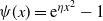$\psi(x)=\textrm{e}^{\eta x^2}-1$ , $0<\alpha \lt 2$ , $0<\eta<\frac{1}{2}$ . Using [Reference Friz and Victoir14, Theorem A.19], there exists $c=c(\alpha)$ such that

\begin{equation*}\mathbb E\exp\left\{c\eta\sup_{t,s\in[0,1]}\frac{|\mathbb{Y}_{\epsilon}(t)-\mathbb{Y}_{\epsilon}(s)|^{2}}{|t-s|^{\alpha'}}\right\}<\infty,\end{equation*}

where $0<\alpha'<\alpha$ . Hence, for any $L>0$ , it follows that

\begin{align*}&\limsup_{\delta\to0}\limsup_{\epsilon\to0}\lambda^{2}_{\epsilon}\log\mathbb P\left\{\sup_{|t-s|<\delta}|\lambda_{\epsilon}\mathbb{Y}_{\epsilon}(t)-\lambda_{\epsilon}\mathbb{Y}_{\epsilon}(s)|>L\right\}\\[4pt] &\leq \limsup_{\delta\to0}\limsup_{\epsilon\to0}\lambda^{2}_{\epsilon}\left(-\frac{c\eta L^2}{\lambda_{\epsilon}^2\delta^{\alpha'}}+\log\mathbb E\exp\left\{c\eta\sup_{t,s\in[0,1]}\frac{|\mathbb{Y}_{\epsilon}(t)-\mathbb{Y}_{\epsilon}(s)|^{2}}{|t-s|^{\alpha'}}\right\}\right)\\[4pt] &=-\infty,\end{align*}

which implies the exponential tightness of $\{\lambda_{\epsilon}\mathbb{Y}_{\epsilon},\epsilon>0\}$ ; i.e. for any $L>0$ , there exists a compact set $\mathcal K_{L}\subset C([0,1])$ such that $\limsup_{\epsilon\to0}\lambda^{2}_{\epsilon}\log\mathbb P\big(\lambda_{\epsilon}\mathbb{Y}_{\epsilon}\in\mathcal K^{c}_{L}\big) \leq -L$ .

Since G is strictly increasing and continuous, $\tilde{\mathcal K}_{L}\,:\!=\,\big\{f: f=g\circ G \text{ for some } g\in\mathcal K_{L}\big\}$ is also a compact set in C([0,1]) and $h\in\tilde{\mathcal K}_{L}$ if and only if $h\circ G^{-1}\in\mathcal K_{L}$ . Therefore, $\limsup_{\epsilon\to0}\lambda^{2}_{\epsilon}\log\mathbb P\big(\lambda_{\epsilon}Y_{\epsilon}\in\tilde{\mathcal K}^{c}_{L}\big) \leq \limsup_{\epsilon\to0}\lambda^{2}_{\epsilon}\log\mathbb P\big(\lambda_{\epsilon}\mathbb{Y}_{\epsilon}\in\mathcal K^{c}_{L}\big) \leq -L$ , which implies the desired result.

Proof of Theorem 1.1. By Propositions 3.1 and 3.2, the family $\{\lambda_{\epsilon}Y_{\epsilon},\epsilon>0\}$ satisfies the sample path moderate deviation in C([0,1]) with uniform topology, with speed $\lambda^{2}_{\epsilon}$ and rate function $\widetilde{I}(\cdot)$ defined by

\begin{equation*}\widetilde{I}(f)=\sup_{k\in\mathbb{N}}\sup_{0\leq t_1\leq\cdots\leq t_k}J_{t_1,\ldots, t_k}\big(f(t_1),\ldots,f(t_k)\big), \qquad f\in C([0,1]),\end{equation*}

where $J_{t_1,\ldots, t_k}(\cdot)$ is defined in Proposition 3.1.

To end the proof of this theorem, we only need to show $\widetilde{I}(f)=I(f)$ for $f\in C([0,1])$ , where $I(\cdot)$ is defined by (3). In fact, by [Reference Deuschel and Stroock11, Theorem 3.4.5] or the weak convergence approach introduced in [Reference Bouè6, Reference Budhiraja, Dupuis and Maroulas7], $\big\{\lambda_{\epsilon}\int^{1}_{0}K(t,r) \, \textrm{d} W_{r}, t\in[0,1]\big\}$ satisfies the sample path moderate deviations with speed $\lambda_{\epsilon}^2$ and rate function $I(\cdot)$ . Moreover, it is noted that the rate function for the finite-dimensional vector $\big\{\lambda_{\epsilon}\big(\int^{1}_{0}K(t_1,r) \textrm{d} B_{r},\ldots,\int^{1}_{0}K(t_k,r) \textrm{d} B_{r}\big)$ , $\epsilon>0\big\}$ is just $J_{t_1,\ldots, t_k}(\cdot)$ . Therefore, by the Dawson–Gärtner projective limits theorem and exponential tightness [Reference Dembo and Zeitouni10, Theorems 4.6.1, 4.2.4], we have $\widetilde{I}(f)=I(f)$ .