





1. Introduction
We consider a general system of hyperbolic-parabolic balance laws,
 \begin{equation}
w_t+f(w)_x=[B(w)w_x]_x+r(w),\quad x\in\mathbb{R},\,\,t\in\mathbb{R}^+,
\end{equation}
where  $w,f,r\in\mathbb{R}^n$ and
 $B\in\mathbb{R}^{n\times n}$. Here,
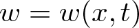 $w=w(x,t)$ is the unknown density function with components representing mass density, momentum density, etc.;
 $f$ is the flux function; and
 $r$ represents external forces, relaxation, chemical reaction, and so forth. The matrix
 $B$ is known as a viscosity matrix. It is for viscosity, heat conduction, species diffusion, etc. We are interested in the Cauchy problem of (1.1) with the initial condition
 \begin{equation}
w(x,0)=w_0(x), \qquad x\in\mathbb{R}.
\end{equation}
Many interesting physical models take the form (1.1). Usually, the flux function satisfies an entropy condition so that the corresponding inviscid form
 \begin{equation}
w_t+f(w)_x=0
\end{equation}
is hyperbolic [Reference Friedrichs and Lax5]. On the other hand, the viscosity matrix is rank deficient as dictated by physics. Examples are those from continuum mechanics with a continuity equation. Thus, (1.1) is hyperbolic-parabolic rather than uniformly parabolic. The appearance of the lower-order term makes (1.1) a system of balance laws rather than conservation laws. In many physical applications, the Jacobian matrix of the lower-order term is also rank deficient. An appropriate set of structural conditions needs to be imposed on (1.1) so that there is sufficient coupling among its equations to have dissipation of solutions.
An important example of (1.1) is polyatomic gas flows in both translational and vibrational non-equilibrium [Reference Clarke and McChesney4, Reference Vincenti and Kruger21],
 \begin{equation}
\begin{cases}
\rho_t+(\rho u)_x=0,\\
(\rho u)_t+(\rho u^2+p)_x=(\mu u_x)_x,\\
(\rho E)_t+(\rho Eu+pu)_x=(\mu uu_x+\kappa T_{1x}+\nu \rho e_{2x})_x,\\
(\rho e_2)_t+(\rho e_2u)_x=(\nu\rho e_{2x})_x+\rho\frac{e_2^*-e_2}{\tau}.
\end{cases}
\end{equation}
Here,  $\rho$,
 $u$ and
 $p$ are the density, velocity and pressure, respectively. The total specific energy is
 \begin{equation}
E=e+\frac12 u^2,\qquad e=e_1+e_2,
\end{equation}
where the internal energy  $e$ consists of two parts:
 $e_2$ is the non-equilibrium vibrational energy, and
 $e_1$ is the rest of the internal energy.
The dissipation parameters are the viscosity coefficient  $\mu$, the thermal conductivity
 $\kappa$, and the self-diffusion coefficient
 $\nu$. They are introduced to compensate for the non-equilibrium in the translational mode through the Chapman–Enskog expansion. On the other hand, the vibrational mode is singled out as the non-equilibrium mode. Such a setup is based on the fact that the relaxations from translational non-equilibrium and from vibrational non-equilibrium to their respective local equilibrium states are on very different time scales.
Therefore, we need two sets of thermodynamic variables. One is for the translational mode and for all other internal modes that are at the same pace with the translational mode, and the other is for the vibrational mode exclusively. We use subscript ‘1’ for the former and ‘2’ for the latter, like  $e_1$ and
 $e_2$ introduced above. Thus,
 $T_1$ in (1.4) stands for the translational temperature. In (1.4), we use
 $e_2^*$ for the local equilibrium value of
 $e_2$ and
 $\tau$ for the vibrational relaxation time scale. Both
 $e_2^*$ and
 $\tau$ are known functions of the thermodynamic variables of set one.
The two sets of thermodynamic variables obey two different thermodynamic equations:
 \begin{equation}
T_1ds_1=de_1+pdv, \qquad v=1/\rho,
\end{equation}
 \begin{equation}
T_2ds_2=de_2.
\end{equation}
Here,  $v$ is the specific volume,
 $T_2$ is the vibrational temperature, and
 $s_1$ and
 $s_2$ are the translational and vibrational entropies, respectively. The total entropy is
 \begin{equation}
s=s_1+s_2.
\end{equation}
From (1.6) and (1.7), two of the thermodynamic variables in set one are independent, and one in set two is independent. Therefore, (1.4) is a closed system of those variables and  $u$.
Recently, Aoki et al. proposed a two-temperature Navier–Stokes type model for polyatomic gas flows [Reference Aoki, Bisi, Groppi and Kosuge22]. The system is derived from the polyatomic version of the ellipsoidal-statistical model rather than the original Boltzmann equation. In one space dimension, the model reads
 \begin{equation}
\begin{cases}
\rho_t+(\rho u)_x=0,\\
(\rho u)_t+(\rho u^2+\rho RT_1)_x=(\mu_{\rm tr} u_x)_x,\\
[\rho (\frac{3+D}2RT\!+\!\frac12 u^2)]_t\!+\![\rho u(\frac{3+D}2RT\!+\!RT_1+\frac12 u^2)]_x=[\frac25\lambda_{\rm tr}(\frac{3+D}2T_x\!+\!T_{1x})\!+\!\mu_{\rm tr}u u_x]_x,\\
(\rho T_2)_t+(\rho uT_2)_x=\frac2{D R}(\lambda_{\rm int}T_{2x})_x+\theta A_c(T)\rho^2(T-T_2).
\end{cases}
\end{equation}
Here,  $\rho$ and
 $u$ are the density and velocity, respectively, as in (1.4). Meanwhile,
 $T_1$ and
 $T_2$ are the temperatures of the translational mode and internal modes, respectively.
 $R$ is the gas constant per unit mass, while
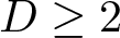 $D\ge2$ is a constant for the number of internal degrees of freedom of gas molecules. The temperature
 $T$ is
 \begin{equation}
T=\frac{3T_1+D T_2}{3+D}.
\end{equation}
The viscosity coefficient and the thermal conductivities for the translational temperature and for the internal temperature are
 \begin{equation}
\mu_{\rm tr}=\mu_{\rm tr}(T,T_1),\quad \lambda_{\rm tr}=\lambda_{\rm tr}(T,T_1),\quad\lambda_{\rm int}=\lambda_{\rm int}(T,T_1)=\frac{D}5\lambda_{\rm tr},
\end{equation}
respectively. Also, 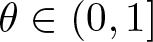 $\theta\in(0,1]$ is a constant parameter, and
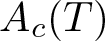 $A_c(T)$ is a function of
 $T$ such that
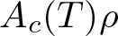 $A_c(T)\rho$ is the collision frequency of the gas molecules.
The setup of (1.9) is different from that of (1.4). Here, the translational mode is separated from  $D$ (at least two) relaxing internal modes. The pressure and the internal energy are
 \begin{equation}
p=\rho RT_1,\quad e=\frac{3+D}2RT=\frac32RT_1+\frac{D}2RT_2\equiv e_1+e_2,
\end{equation}
respectively. Equation (1.9) is a system of four equations for four unknowns 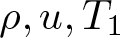 $\rho,u,T_1$ and
 $T_2$, while (1.12) provides related thermodynamic variables.
Both models, (1.4) and (1.9), are examples of the general system (1.1). In fact, as discussed in Section 5, (1.4) and (1.9) are formally very similar. Our main results in this paper apply to both of them.
There are two special cases of (1.1). The first one is  $r=0$ but
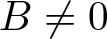 $B\neq0$. It is a system of hyperbolic-parabolic conservation laws,
 \begin{equation}
w_t+f(w)_x=[B(w)w_x]_x.
\end{equation}
Structural conditions for (1.13) are proposed in [Reference Kawashima9, Reference Kawashima and Shizuta11, Reference Shizuta and Kawashima19]. Under those conditions, global well-posedness of (1.13), (1.2) is established for small data solutions [Reference Kawashima9].  $L^2$ time asymptotic behaviour of solutions is studied in [Reference Kawashima10]. Pointwise space-time asymptotic behaviour is studied in [Reference Liu and Zeng14]. As a direct consequence, results in
 $L^p$ spaces,
 $1\le p\le\infty$, are obtained. The innovative approach in [Reference Liu and Zeng14] is a combination of Green’s function estimates for the corresponding linear system and estimates on wave interaction. The approach is extended to other types of problems afterwards [Reference Iguchi and Kawashima7, Reference Liu and Zeng16, Reference Liu and Zeng17, Reference Zeng and Chen24, Reference Zeng26].
The second special case of (1.1) is  $B=0$ but
 $r\neq0$. This is a system of hyperbolic balance laws,
 \begin{equation}
w_t+f(w)_x=r(w).
\end{equation}
There is an extensive literature about (1.14) on structural conditions and global well-posedness, see [Reference Chen, Levermore and Liu3, Reference Hanouzet and Natalini6, Reference Kawashima and Yong12, Reference Yong23] and references therein. In particular, a set of structural conditions is proposed in [Reference Zeng29], which simplifies the set proposed in [Reference Kawashima and Yong12] and is parallel to those conditions developed for (1.13) in [Reference Kawashima9, Reference Kawashima and Shizuta11, Reference Shizuta and Kawashima19]. Green’s function estimates are obtained in [Reference Bianchini, Hanouzet and Natalini1, Reference Zeng26]. Pointwise space-time asymptotic behaviour is studied in [Reference Zeng and Chen24], also see [Reference Zeng28].
For the more general system (1.1), rigorous mathematical treatments are much more recent. Although its counterparts in multi-space dimensions, with space dimensions at least three, have been studied in [Reference Kawashima9], the technique used there heavily depends on the fast decay of solutions in higher space dimensions and does not apply to one or two space dimensions. A set of structural conditions for (1.1) is proposed in [Reference Zeng31]. It is a natural extension of the classical works in [Reference Kawashima9, Reference Kawashima and Shizuta11, Reference Shizuta and Kawashima19] for (1.13). It reduces to those conditions in the special case (1.13), and to the set proposed in [Reference Zeng29] in the case of (1.14) as well. The set is proposed for all space dimensions and applicable to the physical model of polyatomic gas flows in both translational and vibrational non-equilibrium.
Under the structural conditions proposed in [Reference Zeng31], a general  $L^2$ theory for small, classical solutions to (1.1), (1.2) and to its multi-dimensional counterparts has been developed in recent years. This includes global existence via the energy method in [Reference Zeng31] for all space dimensions, and
 $L^p$ (
 $p\ge2$) time decay in [Reference Zeng32] for multi-space dimensions and in [Reference Zeng34] for one space dimension. Time asymptotic behaviour of solutions in multi-space dimensions is studied in [Reference Zeng33].
The result of time asymptotic behaviour for multi-space dimensions obtained in [Reference Zeng33] does not apply to one space dimension. This is because plane wave solutions have less space to diffuse and hence the time decay is slower. The asymptotic behaviour of solutions has an intrinsically different picture in one space dimension than in multi-space dimensions, where the phenomenon is basically linear. In one space dimension, by contrast, an asymptotic solution of (1.1), (1.2) necessarily includes Burgers waves if the reduced characteristic fields are genuinely nonlinear.
A roadmap for studying the solution behaviour of (1.1), (1.2) in depth is as follows. One first considers the linearized system of (1.1) around a constant equilibrium state  $\bar w$, with
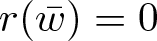 $r(\bar w)=0$. It reads
 \begin{equation}
w_t+Aw_x=Bw_{xx}+Lw,
\end{equation}
where
 \begin{equation}
A=f'(\bar w),\quad B=B(\bar w),\quad L=r'(\bar w).
\end{equation}
The goal of this part is to obtain detailed estimates on the Green’s function. It is done under the linear version of the structural conditions proposed in [Reference Zeng31]. One first finds the Green’s function in the Fourier space as the solution matrix of an ODE system. Then estimates on the inverse transform are carried out to obtain a formulation of the Green’s function in the physical space. The formulation is explicit in leading terms, using coefficients of (1.15), and precise and detailed in higher-order terms.
The second part of studying the solution behaviour is to write (1.1) as a linear system with nonlinear source terms. Based on properties of the flux function  $f$ and information contained in the Green’s function estimates, one constructs an asymptotic component for each characteristic field. After extracting the explicit, predetermined asymptotic solution, one presents the remainder using Duhamel’s principle. Estimation on wave interaction then follows. The expected results are space-time estimates on the remainder, which further imply
 $L^p$,
 $1\le p\le\infty$, convergence rates of the remainder.
While the above roadmap is along the lines of the special cases (1.13) and (1.14), see [Reference Liu and Zeng14, Reference Zeng and Chen24], the analysis is much more complicated here due to the intricate interwinding of the matrices  $A$,
 $B$ and
 $L$ in the Green’s function of (1.15). The involvement of
 $f$ in the construction of an asymptotic solution in the second part of the roadmap adds additional difficulties. Due to the great complexity, we focus on obtaining Green’s function estimates for (1.15) in the current paper. Using the results obtained here, we are able to construct a time asymptotic solution to the Cauchy problem of the polyatomic gas flow model (1.4) and study solution behaviour at large time in a recent paper [Reference Zeng35]. The extension of the study of asymptotic behaviour to the general system (1.1), (1.2), however, is left to future work.
The study of Green’s function estimates in the pointwise sense has its own significance in the PDE theory. The original approach developed in [Reference Liu and Zeng14, Reference Liu and Zeng15, Reference Zeng25] for (1.13) has been extended to apply to other problems [Reference Iguchi and Kawashima7, Reference Liu and Zeng17, Reference Rugamba and Zeng18, Reference Shu and Zeng20, Reference Zeng26, Reference Zeng27]. In particular, using rotational invariance, the approach can be extended to study problems in three space dimensions, see [Reference Liu and Yu13, Reference Zeng30] and references therein.
In the current paper, we study Green’s function estimates in the space-time pointwise sense for (1.15) under reasonable and physical assumptions, with applications to the polyatomic gas flow models (1.4) and (1.9). In the special cases when one of the matrices  $L$ and
 $B$ becomes zero, our results reduce to those obtained in [Reference Liu and Zeng14] for hyperbolic-parabolic conservation laws and in [Reference Zeng26] for hyperbolic balance laws.
Our focus in the current study is on the new challenge of the intertwining of the three coefficient matrices  $A$,
 $B$ and
 $L$. These matrices together with their coupling determine various parameters in the leading terms of the Green’s function. The parameters are to be found employing ideas from Kato’s perturbation theory [Reference Kato8] and from Chapman–Enskog expansions.
The plan of the paper is as follows. In Section 2, we set up our problem, impose hypotheses, and state main results. In Section 3, we consider the Green’s function in the Fourier space and carry out the corresponding spectral analysis. Parameters in the leading terms are obtained in this section. In Section 4, we study the inverse Fourier transform and prove the main results. In Section 5, we apply our results to the polyatomic gas flow models (1.4) and (1.9). Finally, in the Appendix we list some alternative steps in finding parameters in the leading terms of the Green’s function.
2. Main results
In this section, we consider the general linear system (1.15),
 \begin{equation}
w_t+Aw_x=Bw_{xx}+Lw,\qquad x\in\mathbb{R},\quad t\in\mathbb{R}^+,
\end{equation}
where 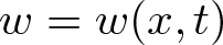 $w=w(x,t)$ is an
 $n$-vector, and
 $A,B,L\in\mathbb{R}^{n\times n}$ are constant matrices. As dictated by physics,
 $B$ and
 $L$ usually are rank deficient. We are interested in the Green’s function for the Cauchy problem of (2.1).
For this, we impose the following structural conditions.
Assumption 2.1. (i) There exists a symmetric, positive definite matrix  $A_0$, such that
 $A_0A$ is symmetric,
 $A_0B$ is symmetric, positive semi-definite, and
 $A_0L$ is symmetric, negative semi-definite.
(ii) There are  $n_1$ conservation laws in (2.1). That is, there is a partition
 $n=n_1+n_2$,
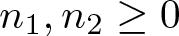 $n_1,n_2\ge0$, such that
 \begin{equation}
L=\begin{pmatrix}0_{n_1\times n_1}&0_{n_1\times n_2}\\L_{21}&L_{22}\end{pmatrix},
\end{equation}
where  $L_{21}\in\mathbb{R}^{n_2\times n_1}$ and
 $L_{22}\in\mathbb{R}^{n_2\times n_2}$ is nonsingular (if
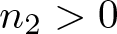 $n_2 \gt 0$).
(iii) Let  $\mathbb N_1$ be the null space of
 $B$ and
 $\mathbb N_2$ be the null space of
 $L$. Then
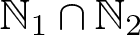 $\mathbb N_1\cap \mathbb N_2$ contains no eigenvectors of
 $A$.
Remark 2.2. In Assumption 2.1, the first hypothesis is for the symmetrizability of (2.1). This is consistent with the entropy condition for a system of nonlinear hyperbolic conservation laws [Reference Friedrichs and Lax5], which is extended to nonlinear hyperbolic-parabolic conservation laws [Reference Kawashima9] and hyperbolic-parabolic balance laws [Reference Zeng31]. The second hypothesis is to set the number of conservation laws in (2.1) to  $n_1$ definitely. It is satisfied by many physical models including the linearizations of (1.4) and (1.9). The third hypothesis is known as the Kawashima–Shizuta condition [Reference Shizuta and Kawashima19]. It implies the full coupling of
 $A$ with
 $B$ and
 $L$ in (2.1), which in turn gives rise to the full dissipation of solutions as seen in the Green’s function estimates.
We now define the Green’s function for the Cauchy problem of (2.1). It is the  $n\times n$ matrix
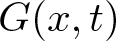 $G(x,t)$ that satisfies
 \begin{equation}
\begin{cases}
G_t+AG_x=BG_{xx}+LG,\\
G(x,0)=\delta(x)I,
\end{cases}
\end{equation}
where  $\delta$ is the Dirac
 $\delta$-function, and
 $I$ is the
 $n\times n$ identity.
For convenience we introduce the following notation for a heat kernel,
 \begin{equation}
H(x,t;\lambda,\mu)=\frac1{\sqrt{4\pi\mu t}}e^{-\frac{(x-\lambda t)^2}{4\mu t}},
\end{equation}
where  $\mu \gt 0$ and
 $\lambda$ are constants.
Theorem 2.3. Let Assumption 2.1 be satisfied and  $l\ge0$ be an integer. For
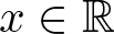 $x\in\mathbb{R}$ and
 $t \gt 0$, the Green’s function
 $G$ of the Cauchy problem of (2.1) satisfies
 \begin{equation}
\begin{aligned}
\frac{\partial^l}{\partial x^l}G(x,t)&=\frac{\partial^l}{\partial x^l}\sum_{j=1}^mH(x,t;\lambda^{(r)}_j,\mu_j)P_j
+O(1)(t+1)^{-\frac12}t^{-\frac l2}\sum_{j=1}^mH(x,t;\lambda^{(r)}_j,C)\\
&+\sum_{j=1}^{m'}e^{-\beta_jt}\sum_{k=0}^l\delta^{(l-k)}(x-\alpha_jt)Q_{j,k}(t).
\end{aligned}
\end{equation}
Here,  $m$ and
 $m'$ are nonnegative integers;
 $\lambda_j^{(r)}$,
 $1\le j\le m$, and
 $\alpha_j$,
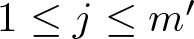 $1\le j\le m'$, are constants;
 $\mu_j$,
 $1\le j\le m$, and
 $\beta_j$,
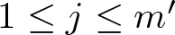 $1\le j\le m'$, are positive constants;
 $P_j$,
 $1\le j\le m$, are constant projections;
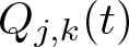 $Q_{j,k}(t)$,
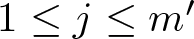 $1\le j\le m'$,
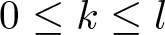 $0\le k\le l$, are
 $n\times n$ matrix-valued polynomials in
 $t$ with degrees not larger than
 $k$;
 $C \gt 0$ is a constant; and
 $\delta$ is the Dirac
 $\delta$-function. The parameters
 $m,m',\lambda_j^{(r)},\alpha_j,\mu_j, \beta_j,P_j$ and
 $Q_{j,0}$ in (2.5) are determined from the coefficient matrices
 $A,B$ and
 $L$ through Procedure 2.9 below and have explicit formulation.
Remark 2.4. In (2.5), there is a singularity  $t^{-\frac{l+1}2}$ at
 $t=0$. Such a singularity is intrinsic if
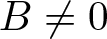 $B\neq0$. (One can think of the heat equation.) On the other hand, if
 $B=0$, i.e., (2.1) is hyperbolic, the singularity is artificial. In this case, (2.5) has an alternative that explicitly excludes the singularity as follows.
Let  $\chi(\mathcal A)$ be the characteristic function of a set
 $\mathcal A$ and
 $\operatorname{sinc}$ be the unnormalized sinc function,
 \begin{equation*}
\operatorname{sinc} x=\frac{\sin x}x.
\end{equation*}
For a pair of large but fixed constants 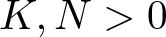 $K,N \gt 0$, if
 $B=0$ in (2.1) then (2.5) can be replaced by
 \begin{equation}
\begin{aligned}
\frac{\partial^l}{\partial x^l}G(x,t)&=\chi(|x|\le Kt)\frac N{\pi}\operatorname{sinc}(Nx)\ast\left[
\frac{\partial^l}{\partial x^l}\sum_{j=1}^mH(x,t;\lambda^{(r)}_j,\mu_j)P_j\right]\\
&+O(1)(t+1)^{-\frac{l+2}2}\sum_{j=1}^me^{-\frac{(x-\lambda_j^{(r)}t)^2}{Ct}}
+\sum_{j=1}^{m'}e^{-\beta_jt}\sum_{k=0}^l\delta^{(l-k)}(x-\alpha_jt)Q_{j,k}(t)
\end{aligned}
\end{equation}
for 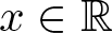 $x\in\mathbb{R}$ and
 $t \gt 0$. Here, the notation ‘
 $\ast$’ means convolution.
We notice that in the first term of (2.6), the singularity  $t^{-\frac{l+1}2}$ from derivatives of heat kernels is eliminated through the convolution with the
 $\operatorname{sinc}$ function. This can be seen by integration by parts and properties of the
 $\operatorname{sinc}$ function and heat kernels.
In the case  $B=0$, while (2.6) is more accurate, (2.5) is much easier to apply since every term on the right-hand side is locally defined. At the same time, in the application to nonlinear systems through Duhamel’s principle, the singularity
 $t^{-\frac{l+1}2}$ in (2.5) can be bypassed via integration by parts [Reference Zeng and Chen24, Reference Zeng26, Reference Zeng27]. More specifically, the
 $l$-th derivative of
 $G$ is used to estimate
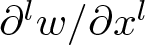 $\partial^lw/\partial x^l$. From PDE theory, the initial data
 $w_0$ is necessary to have at least the same regularity. Thus, the contribution from initial data can be expressed as convolutions
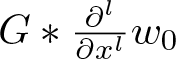 $G\ast\frac{\partial^l}{\partial x^l}w_0$ and
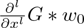 $\frac{\partial^l}{\partial x^l}G\ast w_0$ through integration by parts. We then divide the temporal domain
 $t \gt 0$ as two parts,
 $(0,1]\cup[1,\infty)$. For
 $t\le1$ we use
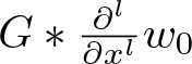 $G\ast\frac{\partial^l}{\partial x^l}w_0$ since time-decay rates are not a concern,
 $O(1)=O(1)(t+1)^{-l/2}$. On the other hand, for
 $t\ge1$ we use
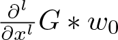 $\frac{\partial^l}{\partial x^l}G\ast w_0$ to obtain the wanted time decay, noting
 $t^{-l/2}=O(1)(t+1)^{-l/2}$. A similar technique is used to handle the contribution from nonlinear source terms. When linearizing (1.1), nonlinear source terms inherit the same regularity from
 $w$.
Remark 2.5. The first term on the right-hand side of (2.5) is the leading term and represents the contribution from the equilibrium system. This can be seen by considering the system
 \begin{equation}
w_t+Aw_x=\varepsilon Bw_{xx}+\frac1{\varepsilon}Lw
\end{equation}
and its Green’s function 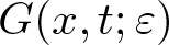 $G(x,t;\varepsilon)$. By a rescaling one has
 $G(x,t;\varepsilon)=\frac1{\varepsilon}G(x/\varepsilon, t/\varepsilon;1)$. Now let
 $\varepsilon\rightarrow0^+$. The second and third terms on the right-hand side of (2.5) (with
 $l=0$) disappear while the first term survives and its heat kernels become
 $\delta$-functions. In this case, (2.7) is reduced to the inviscid, equilibrium system of (2.1) and
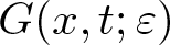 $G(x,t;\varepsilon)$ approaches to its Green’s function.
The formulation of parameters in (2.5) is an application of a reduction process in Kato’s perturbation theory [Reference Kato8]. It has an intricate intertwining of the three matrices  $A,B$ and
 $L$. To make our formulation more manageable, we first introduce new variables to reduce
 $L$ in (2.2) to a block diagonal structure.
For our convenience, we introduce notations as follows for a partition of a matrix  $Z\in\mathbb{R}^{n\times n}$ according to (ii) of Assumption 2.1. We write
 \begin{equation}
Z=\begin{pmatrix}Z_{11}& Z_{12}\\ Z_{21}& Z_{22}\end{pmatrix},
\end{equation}
where  $Z_{11}\in\mathbb{R}^{n_1\times n_1}$,
 $Z_{12}\in\mathbb{R}^{n_1\times n_2}$,
 $Z_{21}\in\mathbb{R}^{n_2\times n_1}$ and
 $Z_{22}\in\mathbb{R}^{n_2\times n_2}$.
We introduce new variables also according to (ii) of Assumption 2.1. Let
 \begin{equation}
\begin{aligned}
&w=\begin{pmatrix}w_1\\w_2\end{pmatrix},\qquad w_1\in\mathbb{R}^{n_1},\,\,w_2\in\mathbb{R}^{n_2};\\
&\tilde w=\begin{pmatrix}w_1\\L_{21}w_1+L_{22}w_2\end{pmatrix}
\equiv\begin{pmatrix}\tilde w_1\\ \tilde w_2\end{pmatrix}.
\end{aligned}
\end{equation}
Here, we have used the partition (2.8) for  $L$.
From (ii) of Assumption 2.1,  $L_{22}$ is invertible. We thus have
 \begin{equation}
\tilde w_w=\begin{pmatrix}I_{n_1\times n_1}&0_{n_1\times n_2}\\L_{21}&L_{22}\end{pmatrix},\qquad
w_{\tilde w}=\tilde w_w^{-1}=\begin{pmatrix}I_{n_1\times n_1}&0_{n_1\times n_2}\\-L_{22}^{-1}L_{21}&L_{22}^{-1}\end{pmatrix}.
\end{equation}
Noting  $\tilde w=\tilde w_ww$, from (2.1), we have the equation for
 $\tilde w$ as follows,
 \begin{equation}
\tilde w_t+\tilde A\tilde w_x=\tilde B\tilde w_{xx}+\tilde L\tilde w,
\end{equation}
where
 \begin{equation}
\tilde A=\tilde w_wAw_{\tilde w},\quad\tilde B=\tilde w_wBw_{\tilde w},\quad\tilde L=\tilde w_wLw_{\tilde w}.
\end{equation}
Let
 \begin{equation}
\tilde A_0=w_{\tilde w}^tA_0w_{\tilde w}.
\end{equation}
Then
 \begin{equation}
\tilde A_0\tilde A=w_{\tilde w}^tA_0Aw_{\tilde w},\qquad\tilde A_0\tilde B=w_{\tilde w}^tA_0Bw_{\tilde w},\qquad\tilde A_0\tilde L=w_{\tilde w}^tA_0Lw_{\tilde w}.
\end{equation}
Thus, under Assumption 2.1,  $\tilde A_0$ is symmetric, positive definite;
 $\tilde A_0\tilde A$ is symmetric;
 $\tilde A_0\tilde B$ is symmetric, positive semi-definite; and
 $\tilde A_0\tilde L$ is symmetric, negative semi-definite. One can show that the intersection of null spaces of
 $\tilde B$ and
 $\tilde L$ contains no eigenvectors of
 $\tilde A$. On the other hand, (ii) in Assumption 2.1 implies
 \begin{equation*}
\tilde L=\tilde w_wLw_{\tilde w}=\begin{pmatrix}0_{n_1\times n_1}&0_{n_1\times n_2}\\0_{n_2\times n_1}&L_{22}\end{pmatrix}
\end{equation*}
by (2.10) and (2.12). Therefore, in the new system (2.11) for the new variable  $\tilde w$, all coefficient matrices satisfy Assumption 2.1, with a simplified, block-diagonal form of
 $\tilde L$.
The block-diagonal form of  $\tilde L$ greatly simplifies the formulation of parameters in our main estimate (2.5). At the same time, the Green’s function
 $\tilde G$ for (2.11) is related to
 $G$ for (2.1) by
 \begin{equation}
\tilde G(x,t)=\tilde w_wG(x,t)w_{\tilde w},
\end{equation}
and hence  $G$ can be easily recovered from
 $\tilde G$. Therefore, we drop the tilde accent, and consider (2.1) with a simplified
 $L$.
Assumption 2.1’. (i) There exists a symmetric, positive definite matrix  $A_0$, such that
 $A_0A$ is symmetric,
 $A_0B$ is symmetric, positive semi-definite, and
 $A_0L$ is symmetric, negative semi-definite.
(ii) The matrix  $L$ has a block-diagonal form
 \begin{equation}
L=\operatorname{diag} (0_{n_1\times n_1},L_{22}),
\end{equation}
where  $L_{22}\in\mathbb{R}^{n_2\times n_2}$ is invertible.
(iii) Let  $\mathbb N_1$ be the null space of
 $B$ and
 $\mathbb N_2$ be the null space of
 $L$. Then
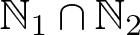 $\mathbb N_1\cap \mathbb N_2$ contains no eigenvectors of
 $A$.
Next, we cite some known results under Assumption 2.1’.
Lemma 2.6. ([Reference Zeng and Chen24])
Under (i) and (ii) of Assumption 2.1’,  $A_0$ is block-diagonal in the partition of (2.8),
 \begin{equation}
A_0=\operatorname{diag}(A^0_{11},A^0_{22}).
\end{equation}
Lemma 2.7. Under (i) of Assumption 2.1’, the matrices  $A,B$ and
 $L$ are diagonalizable with real eigenvalues. The eigenvalues of
 $B$ are nonnegative, and the eigenvalues of
 $L$ are nonpositive.
Lemma 2.6 is easily verified by comparing  $A_0L$ and
 $L^tA_0$, using (2.16). For Lemma 2.7, we observe that
 $A$ is similar to
 \begin{equation}
A_0^{\frac12}A(A_0^{\frac12})^{-1}=(A_0^{\frac12})^{-1}(A_0A)(A_0^{\frac12})^{-1},
\end{equation}
where  $A_0^{\frac12}$ is a square root of
 $A_0$, chosen as symmetric, positive definite. The right-hand side of (2.18) is symmetric and hence diagonalizable with real eigenvalues under (i) of Assumption 2.1’. We can discuss
 $B$ and
 $L$ similarly.
Let
 \begin{equation}
A^{(r)}=A_{11}\in\mathbb{R}^{n_1\times n_1},
\end{equation}
which is the part of  $A$ related to the reduced system (the equilibrium system). From (2.17), we have
 \begin{equation*}
A_0A=\begin{pmatrix}A^0_{11}A^{(r)}&A^0_{11}A_{12}\\A^0_{22}A_{21}&A^0_{22}A_{22}\end{pmatrix}.
\end{equation*}
Under (i) of Assumption 2.1’,  $A_0A$ is symmetric,
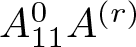 $A^0_{11}A^{(r)}$ is also symmetric. Noting
 $A_0$ is symmetric, positive definite, so is
 $A^0_{11}$. Thus, following the discussion above for Lemma 2.7, we have
Lemma 2.8. Under (i) of Assumption 2.1’,  $A^{(r)}$ is diagonalizable with real eigenvalues.
Now we formulate the parameters in our main estimate (2.5) under Assumption 2.1’. For simplicity, we assume that all eigenvalues of  $A^{(r)}$ are simple in the following procedure, and postpone the formulation related to multiple eigenvalues to Appendix A.
Procedure 2.9.
The parameters in (2.5) are evaluated as follows.
Step 1. Assume that all eigenvalues of  $A^{(r)}$ are simple,
 \begin{equation*}
\lambda^{(r)}_1 \lt \lambda^{(r)}_2 \lt \cdots \lt \lambda^{(r)}_{n_1}.
\end{equation*}
These are  $\lambda^{(r)}_j$ in (2.5), and
 $m=n_1$ therein. Let the normalized left eigenvector (row vector) and right eigenvector of
 $A^{(r)}$ corresponding to
 $\lambda^{(r)}_j$ be
 $l^{(r)}_j$ and
 $r^{(r)}_j$, respectively,
 \begin{equation*}
\begin{aligned}
&A^{(r)}r^{(r)}_j=\lambda^{(r)}_jr^{(r)}_j,\qquad l^{(r)}_jA^{(r)}=\lambda^{(r)}_jl^{(r)}_j,\qquad 1\le j\le n_1,\\
&\begin{pmatrix}l^{(r)}_1\\ \vdots\\l^{(r)}_{n_1}\end{pmatrix}\begin{pmatrix}r^{(r)}_1&\cdots&^{(r)}_{n_1}\end{pmatrix}=I_{n_1\times n_1}.
\end{aligned}
\end{equation*}
Then corresponding to each  $\lambda^{(r)}_j$,
 $P_j$ in (2.5) is given by
 \begin{equation}
P_j=\operatorname{diag}\big(r^{(r)}_jl^{(r)}_j,0_{n_2\times n_2}\big), \qquad1\le j\le n_1.
\end{equation}
Step 2. From Lemma 2.7,  $L$ has spectral decomposition
 \begin{equation}
L=\sum^s_{j=1}-\sigma_jQ_j,
\end{equation}
with 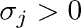 $\sigma_j \gt 0$,
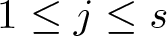 $1\le j\le s$. Here, each
 $-\sigma_j$ is a negative eigenvalue of
 $L$, with the corresponding eigenprojection
 $Q_j$. Let
 $Q_0$ be the eigenprojection corresponding to the eigenvalue zero,
 \begin{equation}
Q_0=I-\sum_{j=1}^sQ_j=\operatorname{diag}(I_{n_1\times n_1}, 0_{n_2\times n_2}).
\end{equation}
Define
 \begin{equation}
S=\sum_{j=1}^s\frac1{\sigma_j}Q_j.
\end{equation}
Then  $-S$ is the value at zero of the reduced resolvent of
 $L$ with respect to the eigenvalue zero. Using (2.16) one can show that
 \begin{equation}
S=\operatorname{diag}(0_{n_1\times n_1},S_{22})
\end{equation}
under the partition (2.8). It is clear that  $S_{22}$ is symmetric, positive definite.
Now for each heat kernel in the first term of (2.5), corresponding to  $\lambda^{(r)}_j$ we have
 \begin{equation}
\begin{aligned}
\mu_j&=(l^{(r)}_j,0_{1\times n_2})(ASA+B)\begin{pmatrix}r^{(r)}_j\\0_{n_2\times1}\end{pmatrix}\\
&=l^{(r)}_j(A_{12}S_{22}A_{21}+B_{11})r^{(r)}_j,\qquad\qquad1\le j\le n_1.
\end{aligned}
\end{equation}
Here, we have applied (2.24). It is shown in Section 3 that 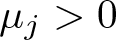 $\mu_j \gt 0$,
 $1\le j\le n_1$.
Step 3. From Lemma 2.7,  $B$ has distinct eigenvalues
 \begin{equation*}
0=\sigma'_0 \lt \sigma'_1 \lt \cdots \lt \sigma'_{s'},
\end{equation*}
with corresponding eigenprojections  $Q'_0,Q'_1,\dots,Q'_{s'}$, and hence
 $B$ has spectral decomposition
 \begin{equation}
B=\sum_{j=1}^{s'}\sigma'_jQ'_j.
\end{equation}
Similar to (2.18), 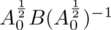 $A^{\frac12}_0B(A_0^{\frac12})^{-1}$ is symmetric. Thus, for
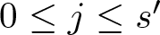 $0\le j\le s'$,
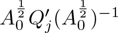 $A^{\frac12}_0Q'_j(A_0^{\frac12})^{-1}$ is symmetric.
Now we form a matrix 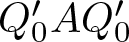 $Q_0'AQ_0'$, which is similar to
 \begin{equation*}
A^{\frac12}_0(Q'_0AQ'_0)(A_0^{\frac12})^{-1}=\big[A^{\frac12}_0Q'_0(A_0^{\frac12})^{-1}\big]\big[A^{\frac12}_0A(A_0^{\frac12})^{-1}\big]\big[A^{\frac12}_0Q'_0(A_0^{\frac12})^{-1}\big].
\end{equation*}
Since the right-hand side is symmetric, 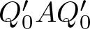 $Q'_0AQ'_0$ is diagonalizable. Next, we have its spectral decomposition in the range of
 $Q'_0$,
 \begin{equation}
Q'_0AQ'_0=\sum_{k=1}^{s^{\prime\prime}}\alpha_k\mathcal{Q}_k, \qquad\sum_{k=1}^{s^{\prime\prime}}\mathcal{Q}_k=Q'_0.
\end{equation}
The distinct eigenvalues  $\alpha_k$ are those appearing in the third term of (2.5).
Step 4. Related to (2.26), we define a matrix
 \begin{equation}
S'=\sum_{j=1}^{s'}\frac1{\sigma'_j}Q'_j,
\end{equation}
which is the value at zero of the reduced resolvent of  $B$ with respect to the eigenvalue zero. Then for each
 $\mathcal{Q}_k$ associated with a distinct
 $\alpha_k$ in (2.27), we form a matrix
 $\mathcal{Q}_k(AS'A-L)\mathcal{Q}_k$ and find its spectral decomposition in the range of
 $\mathcal{Q}_k$,
 \begin{equation}
\mathcal{Q}_k(AS'A-L)\mathcal{Q}_k=\sum_{k'=1}^{s_k}\beta_{kk'}\mathcal{Q}_{kk'},
\qquad
\sum_{k'=1}^{s_k}\mathcal{Q}_{kk'}=\mathcal{Q}_k.
\end{equation}
This is possible since  $\mathcal{Q}_k(AS'A-L)\mathcal{Q}_k$ is diagonalizable via an argument similar to the one that gives (2.27). It is shown in Section 3 that all
 $\beta_{kk'}$ are positive. Now we collect all distinct pairs
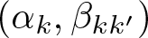 $(\alpha_k, \beta_{kk'})$,
 $1\le k\le s^{\prime\prime}$,
 $1\le k'\le s_k$. The total number of those pairs is
 $m'$ in the third term of (2.5), with
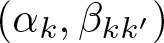 $(\alpha_k,\beta_{kk'})$ being
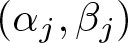 $(\alpha_j,\beta_j)$ and
 $\mathcal{Q}_{kk'}$ being
 $Q_{j,0}$ therein.
In the special case that all  $\alpha_k$ in (2.27) are simple, i.e., all
 $\mathcal{Q}_k$ are rank one, we can simplify Step 4 as Step 4
 $'$ in Appendix A.
Procedure 2.9 is justified in Section 3. In particular, we will show the positivity of  $\mu_j$ and
 $\beta_j$ as a consequence of the crucial assumption of coupling, which is stated in (iii) of Assumption 2.1’.
For an arbitrary vector 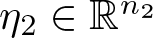 $\eta_2\in\mathbb{R}^{n_2}$ we form a vector
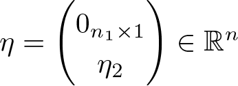 $\eta=\begin{pmatrix}0_{n_1\times 1}\\ \eta_2\end{pmatrix}\in\mathbb{R}^n$. From (2.20), we have
 \begin{equation*}
\eta^tP_j=0,\qquad P_j\eta=0,\qquad1\le j\le n_1.
\end{equation*}
This implies that when  $G$ is multiplied by
 $\eta^t$ from the left, or by
 $\eta$ from the right, the first term (the leading term) on the right-hand side of (2.5) disappears. In this case, we can further refine the higher order term (the second term) in (2.5).
We notice that each  $P_j$ is a subprojection of
 $Q_0$, see (2.20) and (2.22). Thus,
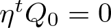
 $\eta$ can be characterized as those satisfying
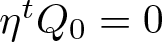 $\eta^tQ_0=0$ or
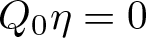 $Q_0\eta=0$. Recall that the formulation of
 $P_j$ and
 $Q_0$ is after the change of variables (2.9), and hence under Assumption 2.1’. Applying (2.15) and (2.10), we recover
 $P_j$ in (2.5) under Assumption 2.1 for the original variables,
 \begin{equation*}
P_j=\tilde w_w^{-1}\begin{pmatrix}r_j^{(r)}l_j^{(r)}&\\ &0_{n_2\times n_2}\end{pmatrix}w^{-1}_{\tilde w}
=\begin{pmatrix}r_j^{(r)}l_j^{(r)}&0_{n_1\times n_2}\\-L_{22}^{-1}L_{21}r_j^{(r)}l_j^{(r)}&0_{n_2\times n_2}\end{pmatrix},\qquad1\le j\le n_1.
\end{equation*}
At the same time, we find the eigenprojection  $Q_0$ of
 $L$ in (2.2) corresponding to the eigenvalue zero as
 \begin{equation*}
Q_0=\begin{pmatrix}I_{n_1\times n_1}&0_{n_1\times n_2}\\-L^{-1}_{22}L_{21}&0_{n_2\times n_2}\end{pmatrix}.
\end{equation*}
It is straightforward to verify that each  $P_j$ is a subprojection of
 $Q_0$. Thus, for
 $\eta$ satisfying
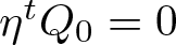 $\eta^tQ_0=0$ or
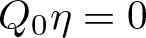 $Q_0\eta=0$, multiplying
 $G$ by
 $\eta^t$ from the left or by
 $\eta$ from the right will eliminate the first term on the right-hand side of (2.5). We now formulate a refinement under such a situation.
Theorem 2.10 Let 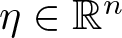 $\eta\in\mathbb{R}^n$ be a constant vector such that
 $\eta^tQ_0=0$, where
 $Q_0$ is the eigenprojection of
 $L$ corresponding to the eigenvalue zero. Then under the same assumptions and same notations as in Theorem 2.3, we have
 \begin{equation}
\begin{aligned}
\frac{\partial^l}{\partial x^l}(\eta^tG)(x,t)&\!=\!\frac{\partial^{l+1}}{\partial x^{l+1}}\sum_{j=1}^mH(x,t;\lambda^{(r)}_j,\mu_j)\eta^t_j
\!+\!O(1)(t\!+\!1)^{-\frac12}t^{-\frac {l+1}2}\sum_{j=1}^mH(x,t;\lambda^{(r)}_j,C)\\
&+\sum_{j=1}^{m'}e^{-\beta_jt}\sum_{k=0}^l\delta^{(l-k)}(x-\alpha_jt)\eta^tQ_{j,k}(t),
\end{aligned}
\end{equation}
where 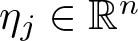 $\eta_j\in\mathbb{R}^n$,
 $1\le j\le m$, are constant vectors. Similarly, if
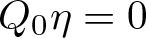 $Q_0\eta=0$ we have
 \begin{equation}
\begin{aligned}
\frac{\partial^l}{\partial x^l}(G\eta)(x,t)&\!=\!\frac{\partial^{l+1}}{\partial x^{l+1}}\sum_{j=1}^mH(x,t;\lambda^{(r)}_j,\mu_j)\eta_j
\!+\!O(1)(t\!+\!1)^{-\frac12}t^{-\frac {l+1}2}\sum_{j=1}^mH(x,t;\lambda^{(r)}_j,C)\\
&+\sum_{j=1}^{m'}e^{-\beta_jt}\sum_{k=0}^l\delta^{(l-k)}(x-\alpha_jt)Q_{j,k}(t)\eta.
\end{aligned}
\end{equation}
3. Spectral analysis
The proofs of Theorems 2.3 and 2.10 consist of two steps. The first step is to perform estimation on the Green’s function  $G$ and its derivatives in the Fourier space via spectral analysis. This is to be done in the current section. At the same time, we also justify Procedure 2.9. In particular, we prove that
 $\mu_j$ and
 $\beta_j$ in (2.5) are positive. The second step is to perform related estimation in the physical space to obtain (2.5), (2.30), and (2.31). This is to be done in Section 4, where we also give an outline of obtaining (2.6)
From the discussion in Section 2, to prove the main estimate (2.5), we only need to prove it under Assumption 2.1’. After that, (2.15) and (2.10) give the intended result under Assumption 2.1 as stated in Theorem 2.3. The simplification makes the formulation of parameters in (2.5) more manageable. To recover the result under Assumption 2.1, we only need to modify the projections  $P_j$ and
 $Q_{j,k}$ via (2.15). Such a simplification also applies to (2.30) and (2.31) in Theorem 2.10 (also to (2.6) in Remark 2.4).
In fact, we can further simplify Assumption 2.1’ in the proof of our main results. For this, again we take  $A_0^{\frac12}$, a square root of
 $A_0$, as a symmetric, positive definite matrix, and write (2.1) in its equivalent form,
 \begin{equation}
\bar w_t+\bar A\bar w_x=\bar B\bar w_{xx}+\bar L\bar w,
\end{equation}
where
 \begin{equation*}
\begin{aligned}
&\bar w=A_0^{\frac12}w,\qquad\bar A=A_0^{\frac12}A(A_0^{\frac12})^{-1},\\
&\bar B=A_0^{\frac12}B(A_0^{\frac12})^{-1},\qquad\bar L=A_0^{\frac12}L(A_0^{\frac12})^{-1}.
\end{aligned}
\end{equation*}
It is straightforward to verify that under Assumption 2.1’, all matrices  $\bar A,\bar B$ and
 $\bar L$ are symmetric, see (2.18). In fact, Assumption 2.1’ is satisfied by
 $\bar A,\bar B$ and
 $\bar L$ (with
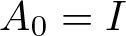 $A_0=I$) as long as it is satisfied by
 $A,B$ and
 $L$.
Note that the Green’s function  $\bar G$ for (3.1) is related to
 $G$ for (2.1) by
 \begin{equation}
\bar G(x,t)=A_0^{\frac12}G(x,t)(A_0^{\frac12})^{-1}.
\end{equation}
Similar to the above discussion on Assumption 2.1 vs. Assumption 2.1’, we can drop the bar accent in (3.1), and study (2.1) under the further simplified version of assumptions.
Assumption 3.1. (i) Let  $A$ be symmetric,
 $B$ be symmetric, positive semi-definite, and
 $L$ be symmetric, negative semi-definite.
(ii) The matrix  $L$ is block-diagonal,
 \begin{equation}
L=\operatorname{diag} (0_{n_1\times n_1},L_{22}),
\end{equation}
where  $L_{22}\in\mathbb{R}^{n_2\times n_2}$ is symmetric, negative definite.
(iii) Let  $\mathbb N_1$ be the null space of
 $B$ and
 $\mathbb N_2$ be the null space of
 $L$. Then
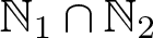 $\mathbb N_1\cap \mathbb N_2$ contains no eigenvectors of
 $A$.
In this section, we carry out Green’s function estimation for (2.1) in the Fourier space under Assumption 3.1. In Section 4, we perform Green’s function estimation in the physical space, also under Assumption 3.1.
Let the Fourier transform of a function  $g(x)$ be
 $\hat g(\xi)$,
 \begin{equation}
\hat g(\xi)=\int_{-\infty}^{\infty}g(x)e^{-ix\xi}\,dx,\qquad g(x)=\frac1{2\pi}\int_{-\infty}^{\infty}\hat g(\xi)e^{ix\xi}\,d\xi.
\end{equation}
Taking the Fourier transform of (2.3) with respect to  $x$ gives us
 \begin{equation}
\begin{cases}\hat G_t+i\xi A\hat G=(i\xi)^2B\hat G+L\hat G,\\ \hat G(\xi,0)=I.\end{cases}
\end{equation}
Solving (3.5), we have
 \begin{equation}
\begin{cases}\hat G(\xi,t)=e^{tE(i\xi)},\\ E(i\xi)=L-i\xi A+(i\xi)^2B.\end{cases}
\end{equation}
Consider
 \begin{equation}
E(z)=L-zA+z^2B
\end{equation}
as a matrix-valued function of a complex variable  $z$. We state some basic facts about its spectral decomposition. They are from complex analysis and perturbation theory, see [Reference Kato8].
First, the number  $n'$ of distinct eigenvalues of
 $E(z)$ is constant if
 $z$ is not one of exceptional points, of which there are only a finite number in the whole complex plane. In each simply connected domain containing no exceptional points, the eigenvalues of
 $E(z)$ can be expressed as
 $n'$ holomorphic functions,
 \begin{equation*}
\tilde\lambda_1(z),\tilde\lambda_2(z),\dots,\tilde\lambda_{n'}(z),
\end{equation*}
which have constant multiplicities  $\tilde m_1,\tilde m_2,\dots,\tilde m_{n'}$, respectively,
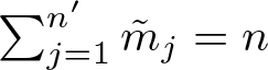 $\sum_{j=1}^{n'}\tilde m_j=n$.
The  $\tilde\lambda_j(z)$,
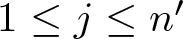 $1\le j\le n'$, are branches of one or several algebraic functions, and are everywhere continuous. These algebraic functions will also be denoted by
 $\tilde\lambda_j(z)$. An exceptional point
 $z_0$ is either a branch point of some of the
 $\tilde\lambda_j(z)$ or a regular point for all of them; in the latter case the values of some of the different
 $\tilde\lambda_j(z)$ coincide at
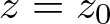 $z=z_0$. Thus, there is always a splitting of eigenvalue at (and only at) an exceptional point.
In general (i.e., without appropriate assumptions),  $E(z)$ in the form of (3.7) is not diagonalizable, and has the spectral representation
 \begin{equation}
E(z)=\sum_{j=1}^{n'}\tilde\lambda_j(z)\tilde P_j(z)+\sum_{j=1}^{n'}\tilde D_j(z)
\end{equation}
for any  $z$ that is not an exceptional point. Here,
 $\tilde P_j(z)$ and
 $\tilde D_j(z)$ are the eigenprojection and the eigennilpotent of
 $\tilde\lambda_j(z)$, respectively,
 \begin{equation}
\begin{aligned}
&\tilde\lambda_j(z)\neq\tilde\lambda_k(z) \quad\mbox{for}\ j\neq k;\\
&\tilde P_j(z)\tilde P_k(z)=\delta_{jk}\tilde P_j(z), \qquad\sum_{j=1}^{n'}\tilde P_j(z)=I;\\
&\tilde D_j^{\tilde m_j}(z)=0,\qquad\tilde P_j(z)\tilde D_j(z)=\tilde D_j(z)\tilde P_j(z)=\tilde D_j(z),\qquad 1\le j,k\le n'.
\end{aligned}
\end{equation}
The eigenprojections  $\tilde P_j(z)$ and the eigennilpotents
 $\tilde D_j(z)$ are also holomorphic in each simply connected domain containing no exceptional points, being branches of one or several analytic functions (also denoted by
 $\tilde P_j(z)$ and
 $\tilde D_j(z)$) and with only algebraic singularities.
The analytic functions  $\tilde P_j(z)$ and
 $\tilde\lambda_j(z)$ have common branch points of the same order. Let
 $z_0$ be an exceptional point. When
 $z$ describes a small circle around
 $z_0$,
 $\{\tilde\lambda_1(z),\tilde\lambda_2(z),\dots,\tilde\lambda_{n'}(z)\}$ and
 $\{\tilde P_1(z), \tilde P_2(z), {\cdot} {\cdot} {\cdot} , \tilde P_{n'}(z)\}$ will undergo the same permutation among themselves after analytic continuation. We emphasize that
 $z_0$ may or may not be a branch point, and
 $\tilde\lambda_j(z)$ is always continuous there, while
 $\tilde P_j(z)$ in general has a pole at
 $z_0$ even when
 $z_0$ is not a branch point. If
 $z_0$ is indeed a branch point, we have the following lemma due to Butler [Reference Butler2], see Theorem 1.9 of Chapter 2 in [Reference Kato8].
Lemma 3.2. If 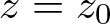 $z=z_0$ is a branch point of
 $\tilde\lambda_j(z)$ (and therefore also of
 $\tilde P_j(z)$) of order
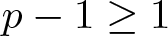 $p-1\ge1$, then
 $\tilde P_j(z)$ has a pole there. That is, the Laurent expansion of
 $\tilde P_j(z)$ in powers of
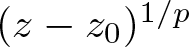 $(z-z_0)^{1/p}$ necessarily contains negative powers.
From (3.7),  $E(z)$ is real, symmetric for real
 $z$. This implies that
 $E(z)$ is diagonalizable on the real axis of the complex plane. Therefore, in (3.8)
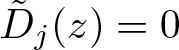 $\tilde D_j(z)=0$,
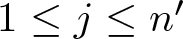 $1\le j\le n'$, on the real axis. By analytic continuation, they are zero on the whole complex plane, and (3.8) is reduced to
 \begin{equation}
E(z)=\sum_{j=1}^{n'}\tilde\lambda_j(z)\tilde P_j(z)
\end{equation}
for every  $z$ that is not an exceptional point.
Since  $E(z)$ is real, symmetric for real
 $z$,
 $\tilde P_j(z)$,
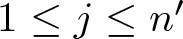 $1\le j\le n'$, are symmetric with
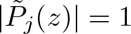 $|\tilde P_j(z)|=1$ on the real axis. By Lemma 3.2, every real
 $z$ is a regular point. In particular,
 $z=0$ is a regular point. Due to the fact that
 $\tilde\lambda_j(z)$ is continuous at
 $z=0$ and
 $\tilde P_j(z)$ does not have a pole there, they are holomorphic at the origin. We thus have their Taylor expansions: for
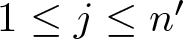 $1\le j\le n'$,
 \begin{equation}
\begin{aligned}
&\tilde\lambda_j(z)=\sum_{k=0}^{\infty}\frac{z^k}{k!}\tilde\lambda_j^{(k)}(0),\\
&\tilde P_j(z)=\sum_{k=0}^{\infty}\frac{z^k}{k!}\tilde P_j^{(k)}(0).
\end{aligned}
\end{equation}
We comment that  $z=0$ is in general an exceptional point. If
 $L$ is rank deficient, as been seen below, the eigenvalue zero of
 $L$ can split into some
 $\tilde\lambda_j(z)$ at the origin. Assumption 3.1 (i), which is a linear version of entropy condition, guarantees that the point is neither a branch point for those
 $\tilde\lambda_j(z)$ nor a pole for the corresponding
 $\tilde P_j(z)$.
Next, we combine (3.7) and (3.10) to have
 \begin{equation}
E(z)=L-zA+z^2B=\sum_{j=1}^{n'}\tilde\lambda_j(z)\tilde P_j(z).
\end{equation}
Setting  $z=0$ gives us
 \begin{equation*}
L=\sum_{j=1}^{n'}\tilde\lambda_j(0)\tilde P_j(0).
\end{equation*}
The spectral decomposition of  $L$ is obtained by combining those terms with the same
 $\tilde\lambda_j(0)$-value. Using the notation (2.21) for the decomposition we write
 \begin{equation}
L=\sum_{j=1}^{n'}\tilde\lambda_j(0)\tilde P_j(0)=\sum_{j=1}^s-\sigma_jQ_j,\qquad \sigma_j \gt 0.
\end{equation}
Thus, we have the following lemma.
Lemma 3.3. The eigenvalues  $\tilde\lambda_j(z)$ and the eigenprojections
 $\tilde P_j(z)$,
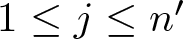 $1\le j\le n'$, of
 $E(z)$ are divided into two groups. In the first group,
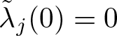 $\tilde\lambda_j(0)=0$ while the corresponding
 $\tilde P_j(0)$ is a sub-projection of
 \begin{equation}
Q_0=I-\sum_{j=1}^sQ_j=\operatorname{diag}(I_{n_1\times n_1},0_{n_2\times n_2}),
\end{equation}
which is the eigenprojection of  $L$ corresponding to the eigenvalue zero, see (2.22). In the second group, each
 $\tilde\lambda_j(0)$ is some
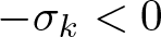 $-\sigma_k \lt 0$,
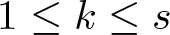 $1\le k\le s$, while
 $\tilde P_j(0)$ is a sub-projection of the corresponding
 $Q_k$.
From Lemma 3.3 and (3.3), it is straightforward to verify the block-diagonal structure of  $\tilde P_j(0)$ as follows.
Lemma 3.4. For the two groups defined in Lemma 3.3, we have the following. In group one,
 \begin{equation}
\tilde P_j(0)=\operatorname{diag}((\tilde P_j(0))_{11},0_{n_2\times n_2}),\qquad\sum_j\tilde P_j(0)=Q_0.
\end{equation}
Here, we have used the partition defined in (2.8). Similarly, in group two,
 \begin{equation}
\tilde P_j(0)=\operatorname{diag}(0_{n_1\times n_1},(\tilde P_j(0))_{22}).
\end{equation}
Now we denote the number of  $\tilde\lambda_j(z)$ (and hence the number of
 $\tilde P_j(z)$) in group one as
 $n'_1$. By appropriately arranging the order, we let the first
 $n'_1$ pairs of
 $\tilde\lambda_j(z)$ and
 $\tilde P_j(z)$ be in group one.
Lemma 3.5. Under the notations in (2.19) and (3.14), we have
 \begin{equation}
-Q_0AQ_0=\sum_{j=1}^{n'_1}\tilde\lambda'_j(0)\tilde P_j(0),\qquad\sum_{j=1}^{n'_1}\tilde P_j(0)=Q_0,
\end{equation}
i.e.
 \begin{equation}
-A^{(r)}=\sum_{j=1}^{n'_1}\tilde\lambda'_j(0)(\tilde P_j(0))_{11},\qquad\sum_{j=1}^{n'_1}(\tilde P_j(0))_{11}=I_{n_1\times n_1}.
\end{equation}
Proof. From (3.12) and (3.9), we have
 \begin{equation}
M(z)\equiv\left(\sum_{j=1}^{n'_1}\tilde P_j(z)\right)E(z)\left(\sum_{j=1}^{n'_1}\tilde P_j(z)\right)=\sum_{j=1}^{n'_1}\tilde\lambda_j(z)\tilde P_j(z).
\end{equation}
Comparing the coefficients of  $z$ on both sides and noting (3.15) give us
 \begin{equation*}
M'(0)=Q_0L\sum_{j=1}^{n'_1}\tilde P'_j(0)-Q_0AQ_0+\sum_{j=1}^{n'_1}\tilde P'_j(0)LQ_0=\sum_{j=1}^{n'_1}\tilde\lambda'_j(0)\tilde P_j(0).
\end{equation*}
By the definition of  $Q_0$, the equation is simplified to
 \begin{equation}
M'(0)=-Q_0AQ_0=\sum_{j=1}^{n'_1}\tilde\lambda'_j(0)\tilde P_j(0).
\end{equation}
By combining terms with the same value of  $\tilde\lambda'_j(0)$, the right-hand side of (3.17) gives us the spectral decomposition of
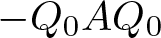 $-Q_0AQ_0$ in the range of
 $Q_0$. Similarly, after such combination, the right-hand side of (3.18) gives us the spectral decomposition of
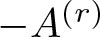 $-A^{(r)}$. In particular,
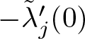 $-\tilde\lambda'_j(0)$ is an eigenvalue of
 $A^{(r)}$.
Let the distinct eigenvalues of  $A^{(r)}$ be
 $\lambda^{(r)}_j$, with multiplicities
 $m_j$,
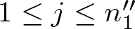 $1\le j\le n^{\prime\prime}_1$,
 $m_1+\cdots+m_{n''}=n_1$. We then divide terms on the right-hand side of (3.17) into groups such that each group has the same value of
 $\tilde\lambda'_j(0)$ and combine each group. This gives us
 \begin{equation}
Q_0AQ_0=\sum_{j=1}^{n_1''}\lambda^{(r)}_j\mathcal P_j,\qquad\sum_{j=1}^{n_1''}\mathcal P_j=Q_0.
\end{equation}
Here, each  $\mathcal P_j$ is an eigenprojection of
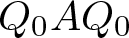 $Q_0AQ_0$ in the range of
 $Q_0$, corresponding to
 $\lambda^{(r)}_j$ and with rank
 $m_j$. By appropriately arranging the order of
 $\tilde\lambda'_j(0)$ in (3.17), we set
 \begin{equation}
\mathcal P_j=\sum_{k=m'_{j-1}+1}^{m'_j}\tilde P_k(0),\qquad1\le j\le n^{\prime\prime}_1,
\end{equation}
where 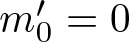 $m'_0=0$ and
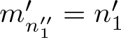 $m'_{n_1''}=n'_1$.
Lemma 3.6. Under the notations of (2.23) and (3.22), for each 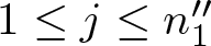 $1\le j\le n^{\prime\prime}_1$ we have
 \begin{equation}
\mathcal P_j(B+ASA)\mathcal P_j=\frac12\sum_{k=m'_{j-1}+1}^{m'_j}\tilde\lambda^{\prime\prime}_k(0)\tilde P_k(0).
\end{equation}
Proof. For  $S$ defined in (2.23) it is straightforward to verify that
 \begin{equation}
LS=SL=-\sum_{j=1}^sQ_j=Q_0-I,\qquad Q_0S=SQ_0=0.
\end{equation}
We now find 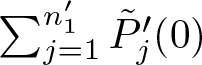 $\sum_{j=1}^{n'_1}\tilde P'_j(0)$. For this, we consider
 \begin{equation}
E(z)\sum_{j=1}^{n'_1}\tilde P_j(z)=\sum_{j=1}^{n'_1}\tilde\lambda_j(z)\tilde P_j(z),
\end{equation}
where we have applied (3.12) and (3.9). Comparing the  $z$-terms on both sides of (3.25) gives us
 \begin{equation*}
L\sum_{j=1}^{n'_1}\tilde P'_j(0)-AQ_0=\sum_{j=1}^{n'_1}\tilde\lambda'_j(0)\tilde P_j(0).
\end{equation*}
Multiplying the resulted equation by  $S$ from the left, we have
 \begin{equation}
SL\sum_{j=1}^{n'_1}\tilde P'_j(0)-SAQ_0=0,
\end{equation}
where we have used (3.24) and the fact that for 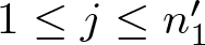 $1\le j\le n'_1$,
 $\tilde P_j(0)$ is a sub-projection of
 $Q_0$. Similarly, we also have
 \begin{equation}\sum_{j=1}^{n'_1}\widetilde P'_j(0)LS-Q_0AS=0.\end{equation}
We sum up (3.26) and (3.27) to have
 \begin{equation}
SL\sum_{j=1}^{n'_1}\tilde P'_j(0)+\sum_{j=1}^{n'_1}\tilde P'_j(0)LS=SAQ_0+Q_0AS.
\end{equation}
Then we substitute  $SL$ and
 $LS$ from (3.24) into (3.28) and simplify. We arrive at
 \begin{equation}
Q_0\sum_{j=1}^{n'_1}\tilde P'_j(0)+\sum_{j=1}^{n'_1}\tilde P'_j(0)Q_0-2\sum_{j=1}^{n'_1}\tilde P'_j(0)
=SAQ_0+Q_0AS.
\end{equation}
Next, we consider the following identity, justified by the definition of eigenprojections as given in (3.9),
 \begin{equation*}
\Bigg[\sum_{j=1}^{n_1'}\tilde P_j(z)\Bigg]
\Bigg[\sum_{j=1}^{n_1'}\tilde P_j(z)\Bigg]=\sum_{j=1}^{n_1'}\tilde P_j(z).
\end{equation*}
Comparing the  $z$-terms on both sides gives us
 \begin{equation*}
\Bigg[\sum_{j=1}^{n_1'}\tilde P_j(0)\Bigg]\Bigg[\sum_{j=1}^{n_1'}\tilde P'_j(0)\Bigg]+\Bigg[\sum_{j=1}^{n_1'}\tilde P'_j(0)\Bigg]
\Bigg[\sum_{j=1}^{n_1'}\tilde P_j(0)\Bigg]=\sum_{j=1}^{n_1'}\tilde P'_j(0).
\end{equation*}
Noting 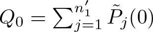 $Q_0=\sum_{j=1}^{n_1'}\tilde P_j(0)$, see (3.17), we write
 \begin{equation}
Q_0\sum_{j=1}^{n'_1}\tilde P'_j(0)+\sum_{j=1}^{n'_1}\tilde P'_j(0)Q_0=\sum_{j=1}^{n'_1}\tilde P'_j(0).
\end{equation}
Substituting (3.30) into (3.29) and simplifying, we arrive at
 \begin{equation}
-\sum_{j=1}^{n'_1}\tilde P'_j(0)
=SAQ_0+Q_0AS.
\end{equation}
Now for  $M(z)$ defined in (3.19), we consider
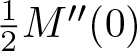 $\frac12M''(0)$. Noting (3.17) and
 $Q_0$ being the eigenprojection of
 $L$ corresponding to the eigenvalue zero, from (3.19), we have
 \begin{equation}
\frac12M''(0)=Q_0BQ_0-Q_0A\sum_{j=1}^{n'_1}\tilde P'_j(0)-\sum_{j=1}^{n'_1}\tilde P'_j(0)AQ_0
+\Bigg[\sum_{j=1}^{n_1'}\tilde P'_j(0)\Bigg]L\Bigg[\sum_{j=1}^{n_1'}\tilde P'_j(0)\Bigg].
\end{equation}
Substituting (3.31) into (3.32) and simplifying, we arrive at
 \begin{align*}
\frac12M''(0)&=Q_0BQ_0+Q_0ASAQ_0+Q_0AQ_0AS+SAQ_0AQ_0\\
&\quad+Q_0ASAQ_0+Q_0ASLSAQ_0.
\end{align*}
Applying (3.24) to the last term on the right, we further have
 \begin{equation}
\frac12M''(0)=Q_0BQ_0+Q_0AQ_0AS+SAQ_0AQ_0+Q_0ASAQ_0.
\end{equation}
With the indexing in (3.22), from (3.19), we have
 \begin{align*}
\Bigg[\sum_{k=m'_{j-1}+1}^{m'_j}\tilde P_k(z)\Bigg]M(z)\Bigg[\sum_{k=m'_{j-1}+1}^{m'_j}\tilde P_k(z)\Bigg]
=\Bigg[\sum_{k=m'_{j-1}+1}^{m'_j}\tilde \lambda_k(z)\tilde P_k(z)\Bigg]\nonumber\\
\Bigg[\sum_{k=m'_{j-1}+1}^{m'_j}\tilde P_k(z)\Bigg]
\end{align*}
for 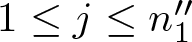 $1\le j\le n^{\prime\prime}_1$. Comparing the
 $z^2$-terms on both sides, noting
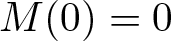 $M(0)=0$ and using the notation in (3.22), we have
 \begin{equation*}
\begin{aligned}
&\frac12\mathcal P_jM''(0)\mathcal P_j+\sum_{k=m'_{j-1}+1}^{m'_j}\tilde P'_k(0)M'(0)\mathcal P_j+\mathcal P_jM'(0)\sum_{k=m'_{j-1}+1}^{m'_j}\tilde P'_k(0)\\
=\,&\frac12\sum_{k=m'_{j-1}+1}^{m'_j}\tilde\lambda^{\prime\prime}_k(0)\tilde P_k(0)\mathcal P_j+\sum_{k=m'_{j-1}+1}^{m'_j}\tilde\lambda'_k(0)\tilde P'_k(0)\mathcal P_j\\
&+\Bigg[\sum_{k=m'_{j-1}+1}^{m'_j}\tilde\lambda'_k(0)\tilde P_k(0)\Bigg]\Bigg[\sum_{k=m'_{j-1}+1}^{m'_j}\tilde P'_k(0)\Bigg].
\end{aligned}
\end{equation*}
Substituting (3.20) into the equation and noting that all  $\tilde\lambda'_k(0)$ on the right-hand side have the same value by our indexing, we simplify the equation to
 \begin{equation}
\frac12\mathcal P_jM''(0)\mathcal P_j=\frac12\sum_{k=m'_{j-1}+1}^{m'_j}\tilde\lambda^{\prime\prime}_k(0)\tilde P_k(0)\mathcal P_j=\frac12\sum_{k=m'_{j-1}+1}^{m'_j}\tilde\lambda^{\prime\prime}_k(0)\tilde P_k(0).
\end{equation}
Finally, we substitute (3.33) into (3.34), noting (3.24) and that each  $\mathcal P_j$ is a sub-projection of
 $Q_0$. This gives us (3.23).
From (3.22) and (3.23), after combining terms of the same value of  $\tilde\lambda^{\prime\prime}_k(0)$, the right-hand side of (3.23) gives us the spectral decomposition of the matrix on the left-hand side in the range of
 $\mathcal P_j$,
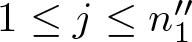 $1\le j\le n^{\prime\prime}_1$. Thus, each
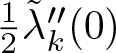 $\frac12\tilde\lambda^{\prime\prime}_k(0)$,
 $m'_{j-1}+1\le k\le m'_j$, is an eigenvalue. Our next lemma shows that these eigenvalues are positive.
Lemma 3.7. For 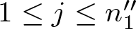 $1\le j\le n^{\prime\prime}_1$,
 $m'_{j-1}+1\le k\le m'_j$, we have
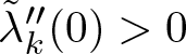 $\tilde\lambda^{\prime\prime}_k(0) \gt 0$.
Proof. For 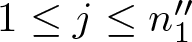 $1\le j\le n^{\prime\prime}_1$ let
 \begin{equation*}
M_j=\mathcal P_j(B+ASA)\mathcal P_j.
\end{equation*}
From (3.23), each 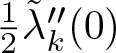 $\frac12\tilde\lambda^{\prime\prime}_k(0)$,
 $m'_{j-1}+1\le k\le m'_j$, is an eigenvalue of
 $M_j$ in the range of
 $\mathcal P_j$. From (2.23),
 $S$ is symmetric, positive semi-definite. Thus,
 $M_j$ is symmetric, positive semi-definite. This implies
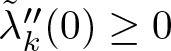 $\tilde\lambda^{\prime\prime}_k(0)\ge0$.
Now we show 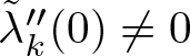 $\tilde\lambda^{\prime\prime}_k(0)\neq0$ by way of contradiction. Suppose
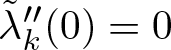 $\tilde\lambda^{\prime\prime}_k(0)=0$. Let
 $v$ be a corresponding eigenvector in the range of
 $\mathcal P_j$,
 \begin{equation}
M_jv=0,\qquad\mathcal P_jv=v\neq0.
\end{equation}
Then
 \begin{equation*}
v^tM_jv=(\mathcal P_jv)^tB(\mathcal P_jv)+(A\mathcal P_jv)^tS(A\mathcal P_jv)
=v^tBv+(Av)^tS(Av)=0.
\end{equation*}
Since  $B$ and
 $S$ are both positive semi-definite, we have
 \begin{equation*}
v^tBv=0,\qquad (Av)^tS(Av)=0,
\end{equation*}
which further implies
 \begin{equation}
Bv=0,\qquad SAv=0.
\end{equation}
Note that  $\mathcal P_j$ is a subprojection of
 $Q_0$, see (3.21). Thus,
 $v$ is in the range of
 $Q_0$ and hence in the null space of
 $L$. Meanwhile, (3.36) shows that
 $v$ is also in the null space of
 $B$. We therefore only need to prove that
 $v$ is an eigenvector of
 $A$ to reach a contradiction to (iii) of Assumption 3.1.
For this, we observe that  $Q_0$ is also the eigenprojection of
 $S$ corresponding to the eigenvalue zero, see (2.23). From (3.36),
 $Av$ is in the null space of
 $S$. Thus,
 \begin{equation*}
Av=Q_0Av.
\end{equation*}
With (3.35) and (3.21), we have
 \begin{equation*}
Av=Q_0A\mathcal P_jv=(Q_0AQ_0)\mathcal P_jv=\lambda_j^{(r)}\mathcal P_jv=\lambda_j^{(r)}v,
\end{equation*}
which shows that  $v$ is an eigenvector of
 $A$.
We combine Lemmas 3.3-3.7 to have a summary on the leading terms as follows. The eigenvalues  $\tilde\lambda_j(z)$, and hence the eigenprojections
 $\tilde P_j(z)$, of
 $E(z)$ are divided into two groups. In the first group, for small
 $z$ eigenvalues split away from the eigenvalue zero of
 $L$,
 \begin{equation}
\tilde\lambda_j(z)=\tilde\lambda'_j(0)z+\frac12\tilde\lambda^{\prime\prime}_j(0)z^2+O(z^3),\qquad1\le j\le n'_1.
\end{equation}
Each  $\tilde P_j(0)$ is a sub-projection of
 $Q_0$, the eigenprojection of
 $L$ corresponding to the eigenvalue zero, and takes the form
 \begin{equation}
\begin{aligned}
&\tilde P_j(0)=\operatorname{diag}\big((\tilde P_j(0))_{11},0_{n_2\times n_2}\big),\quad1\le j\le n'_1,\\
&\sum_{j=1}^{n'_1}(\tilde P_j(0))_{11}=I_{n_1\times n_1}.
\end{aligned}
\end{equation}
The  $\tilde\lambda'_j(0)$,
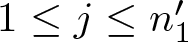 $1\le j\le n'_1$, in (3.37) are eigenvalues of
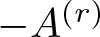 $-A^{(r)}$. In fact,
 \begin{equation}
-A^{(r)}=\sum_{j=1}^{n'_1}\tilde\lambda'_j(0)(\tilde P_j(0))_{11},
\end{equation}
which is equivalent to
 \begin{equation}
-Q_0AQ_0=\sum_{j=1}^{n'_1}\tilde\lambda'_j(0)\tilde P_j(0).
\end{equation}
By combining the terms on the right-hand sides of (3.39) and (3.40) for the same values of  $\tilde\lambda'_j(0)$, we obtain spectral decompositions of
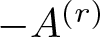 $-A^{(r)}$ and
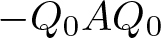 $-Q_0AQ_0$, respectively. Here, the latter is in the range of
 $Q_0$, which gives us
 \begin{equation}
Q_0AQ_0=\sum_{j=1}^{n^{\prime\prime}_1}\lambda^{(r)}_j\mathcal P_j,\qquad
\mathcal P_j=\sum_{k=m'_{j-1}+1}^{m'_j}\tilde P_k(0),\qquad1\le j\le n^{\prime\prime}_1,
\end{equation}
with 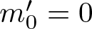 $m'_0=0$ and
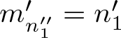 $m'_{n_1''}=n'_1$. Here,
 $\lambda^{(r)}_j$,
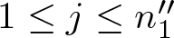 $1\le j\le n^{\prime\prime}_1$, are distinct eigenvalues of
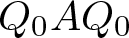 $Q_0AQ_0$ in the range of
 $Q_0$ and hence distinct eigenvalues of
 $A^{(r)}$.
The 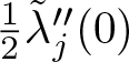 $\frac12\tilde\lambda^{\prime\prime}_j(0)$,
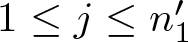 $1\le j\le n'_1$, in (3.37) are positive. In fact, they are nonzero eigenvalues of a symmetric, positive semi-definite matrix. With the notations in (3.41), we have, for
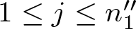 $1\le j\le n^{\prime\prime}_1$,
 \begin{equation}
\mathcal P_j(B+ASA)\mathcal P_j=\sum_{k=m'_{j-1}+1}^{m'_j}\frac12\tilde\lambda^{\prime\prime}_k(0)\tilde P_k(0).
\end{equation}
By combining terms with the same value of  $\tilde\lambda^{\prime\prime}_k(0)$ on the right, we obtain the spectral decomposition for the matrix on the left in the range of
 $\mathcal P_j$. This gives us
 \begin{equation}
\mathcal P_j(B+ASA)\mathcal P_j=\sum_{l=1}^{m^{\prime\prime}_j}\mu_{jl}\mathcal P_{jl},\qquad1\le j\le n^{\prime\prime}_1,
\end{equation}
where each  $\mu_{jl}$ is a distinct
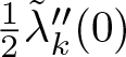 $\frac12\tilde\lambda^{\prime\prime}_k(0)$,
 $m'_{j-1}+1\le k\le m'_j$,
 $\mathcal P_{jl}$ is the sum of the corresponding
 $\tilde P_k(0)$’s that share the same value of
 $\frac12\tilde\lambda^{\prime\prime}_k(0)$, and
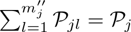 $\sum_{l=1}^{m^{\prime\prime}_j}\mathcal P_{jl}=\mathcal P_j$.
Now we collect all distinct pairs 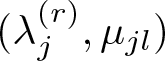 $(\lambda^{(r)}_j, \mu_{jl})$,
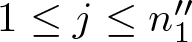 $1\le j\le n^{\prime\prime}_1$,
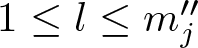 $1\le l\le m^{\prime\prime}_j$. The total number of them is
 \begin{equation}
m=\sum_{j=1}^{n_1''}m^{\prime\prime}_j.
\end{equation}
We rename all  $\mu_{jl}$ and
 $\mathcal P_{jl}$,
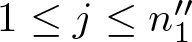 $1\le j\le n_1^{\prime\prime}$,
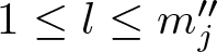 $1\le l\le m_j^{\prime\prime}$, as
 $\mu_j$ and
 $P_j$,
 $1\le j\le m$, respectively. Meanwhile, we let each distinct
 $\lambda^{(r)}_j$ repeat
 $m_j^{\prime\prime}$ times and rename all of them as
 $\lambda^{(r)}_j$,
 $1\le j\le m$. In this way we obtain triples
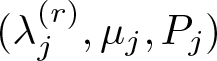 $(\lambda^{(r)}_j,\mu_j,P_j)$,
 $1\le j\le m$.
Using those triples we construct a matrix-valued function
 \begin{equation}
E^*(z)=\sum_{j=1}^m(-\lambda^{(r)}_jz+\mu_jz^2)P_j.
\end{equation}
From the construction of the triples it is clear that
 \begin{equation}
E^*(z)=-zQ_0AQ_0+z^2\sum_{j=1}^{n_1''}\mathcal P_j(B+ASA)\mathcal P_j
=\sum_{j=1}^{n_1'}[\tilde\lambda'_j(0)z+\frac12\tilde\lambda^{\prime\prime}_j(0)z^2]\tilde P_j(0),
\end{equation}
Now we write (3.12) as
 \begin{equation}
E(z)=\sum_{j=1}^{n_1'}\tilde\lambda_j(z)\tilde P_j(z)+\sum_{j=n_1'+1}^{n'}\tilde\lambda_j(z)\tilde P_j(z),
\end{equation}
where the second summation is for eigen-pairs in the second group. In particular, for small  $z$ each
 $\tilde\lambda_j(z)$ in the second summation is perturbed away from a negative eigenvalue of
 $L$, see Lemma 3.3 and (3.13). Therefore, the second summation in (3.47) has a spectral gap and represents exponential decay in
 $G$ in large time.
We compare (3.46) with the first summation in (3.47) to observe that 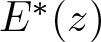 $E^*(z)$ captures the leading term of the summation. Therefore,
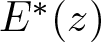 $E^*(z)$ generates the leading term of
 $G$ in large time. We thus define
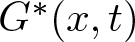 $G^*(x,t)$ through its Fourier transform,
 \begin{equation}
\hat G^*(\xi,t)=e^{tE^*(i\xi)}=\sum_{j=1}^{n_1'}e^{[\tilde\lambda'_j(0)i\xi-\frac12\tilde\lambda^{\prime\prime}_j(0)\xi^2]t}\tilde P_j(0)
{\equiv}
\sum_{j=1}^{m}e^{(-\lambda^{(r)}_ji\xi-\mu_j\xi^2)t}P_j
\end{equation}
in parallel to (3.6). Here, through a consolidation of like terms in the first summation, the last summation of (3.48) defines 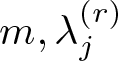 $m,\lambda_j^{(r)}$,
 $\mu_j$ and
 $P_j$ in Theorem 2.3. Taking the inverse Fourier transform gives us
 \begin{equation}
G^*(x,t)=\sum_{j=1}^mH(x,t;\lambda^{(r)}_j,\mu_j)P_j,
\end{equation}
which is the leading term in (2.5) for  $l=0$.
In the special case that all eigenvalues of  $A^{(r)}$ are simple, i.e.,
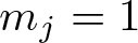 $m_j=1$,
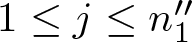 $1\le j\le n_1^{\prime\prime}$, we simplify the formulation of parameters in (3.49) as follows.
From (3.39)-(3.41), we immediately have
 \begin{equation}
n'_1=n^{\prime\prime}_1=n_1,\qquad m'_j=j,\quad1\le j\le n_1.
\end{equation}
Since each  $\mathcal P_j$ in (3.41) is rank-one, (3.42)-(3.44) give us
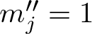 $m^{\prime\prime}_j=1$,
 $1\le j\le n_1$, and
 \begin{equation*}
m=n^{\prime\prime}_1=n_1.
\end{equation*}
Now for each eigenvalue  $\lambda^{(r)}_j$ of
 $A^{(r)}$, let the normalized left eigenvector and right eigenvector of
 $A^{(r)}$ corresponding to
 $\lambda^{(r)}_j$ be
 $l^{(r)}_j$ and
 $r^{(r)}_j$, respectively, see Step 1 in Procedure 2.9. Then (3.38), (3.39) and (3.50) imply that
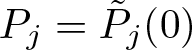 $P_j=\tilde P_j(0)$ is given by (2.20).
From (3.41)-(3.43), we have  $\mathcal P_{j1}=\mathcal P_j=\tilde P_j(0)$ for
 $1\le j\le n_1$ and
 \begin{equation}
\tilde P_j(0)(B+ASA)\tilde P_j(0)=\mu_j\tilde P_j(0).
\end{equation}
Noting 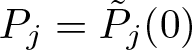 $P_j=\tilde P_j(0)$ is given by (2.20), we multiply (3.51) by
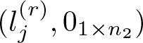 $(l^{(r)}_j,0_{1\times n_2})$ from the left and by
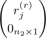 $\begin{pmatrix}r^{(r)}_j\\0_{n_2\times1}\end{pmatrix}$ from the right. This gives us (2.25). Thus, we have justified Steps 1 and 2 in Procedure 2.9.
We have given a detailed spectral analysis of  $E(z)$ for small
 $z$, which induces the leading term
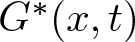 $G^*(x,t)$ of
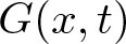 $G(x,t)$ that governs the long-time behaviour. The short-term behaviour, on the other hand, is induced by the spectral analysis of
 $E(z)$ for large
 $z$. It gives rise to the part related to
 $\delta$-functions in (2.5).
We write
 \begin{equation}
E(z)=L-zA+z^2B=z^2(B-\frac1zA+\frac1{z^2}L)\equiv z^2\check E(\frac1z),
\end{equation}
i.e.,
 \begin{equation}
\check E(\check z)=B-\check zA+\check z^2L.
\end{equation}
Here, to consider  $z\rightarrow\infty$ is equivalent to consider
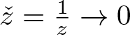 $\check z=\frac1z\rightarrow0$. Noting
 $-\check E$ takes the same form as
 $E$, with the triple
 $(-A,-B,-L)$ corresponds to
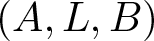 $(A,L,B)$. Under Assumption 3.1, the triple
 $(-A,-B,-L)$ has the same properties as
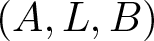 $(A,L,B)$ except that
 $-B$ does not have a block-diagonal structure as
 $L$, see (3.3). Thus, we have similar results for
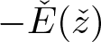 $-\check E(\check z)$ as for
 $E(z)$, except for minor modifications related to the block-diagonal structure of the leading terms in the eigenprojections. We state those results as follows, omitting the proofs as they are parallel to those for
 $E(z)$.
From (3.10) and (3.52), we have
 \begin{equation*}
\check E(\check z)=\check z^2E(\frac1{\check z})=\check z^2\sum_{j=1}^{n'}\tilde\lambda_j(\frac1{\check z})\tilde P_j(\frac1{\check z}).
\end{equation*}
Thus, we have the spectral decomposition for  $\check E(\check z)$ as
 \begin{equation}
\check E(\check z)=\sum_{j=1}^{n'}\check\lambda_j(\check z)\check P_j(\check z),
\end{equation}
where
 \begin{equation*}
\check\lambda_j(\check z)=\check z^2\tilde\lambda_j(\frac1{\check z}),\qquad \check P_j(\check z)=\tilde P_j(\frac1{\check z}),\qquad 1\le j\le n'.
\end{equation*}
Next, from (3.53) and (3.54), we have
 \begin{equation}
B=\sum_{j=1}^{n'}\check\lambda_j(0)\check P_j(0)=\sum_{j=1}^{s'}\sigma_j'Q_j',\qquad\sigma'_j \gt 0,
\end{equation}
where the right hand side is the spectral decomposition of  $B$, obtained by combining terms with the same value of
 $\check\lambda_j(0)$, see (2.26). Since
 $B$ is symmetric, positive semi-definite, we rearrange the order of
 $\check\lambda_j(\check z)$ to have the following lemma.
Lemma 3.8. The eigenvalues  $\check\lambda_j(\check z)$ and the corresponding eigenprojections
 $\check P_j(\check z)$,
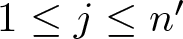 $1\le j\le n'$, of
 $\check E(\check z)$ are divided into two groups. For
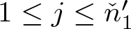 $1\le j\le \check n'_1$, each eigenvalue splits away from the eigenvalue zero of
 $B$ for small
 $\check z$,
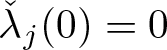 $\check\lambda_j(0)=0$, and the corresponding
 $\check P_j(0)$ is a sub-projection of
 \begin{equation}
Q'_0=I-\sum_{j=1}^{s'}Q'_j=\sum_{j=1}^{\check n'_1}\check P_j(0),
\end{equation}
which is the eigenprojection of  $B$ corresponding to the eigenvalue zero. For
 $\check n'_1+1\le j\le n'$, on the other hand, each
 $\check\lambda_j(0)$ is some
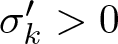 $\sigma'_k \gt 0$, while
 $\check P_j(0)$ is a sub-projection of the corresponding
 $Q'_k$.
Lemma 3.9. With  $Q'_0$ defined in (3.56), we have
 \begin{equation}
-Q'_0AQ'_0=\sum_{j=1}^{\check n'_1}\check\lambda'_j(0)\check P_j(0).
\end{equation}
Lemma 3.9 indicates that  $\check\lambda'_j(0)$,
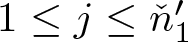 $1\le j\le \check n'_1$, are eigenvalues of
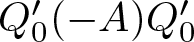 $Q'_0(-A)Q'_0$ when restricted to the range of
 $Q'_0$. By combining terms with the same value of
 $\check\lambda'_j(0)$ on the right , (3.57) gives us the spectral decomposition of
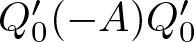 $Q'_0(-A)Q'_0$ in the range of
 $Q'_0$. Thus, letting the distinct
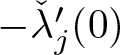 $-\check\lambda'_j(0)$,
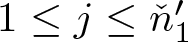 $1\le j\le \check n'_1$, be
 $\alpha_1,\dots,\alpha_{s^{\prime\prime}}$, we have
 \begin{equation}
Q'_0AQ'_0=\sum_{j=1}^{s^{\prime\prime}}\alpha_j\mathcal{Q}_j,\qquad\sum_{j=1}^{s^{\prime\prime}}\mathcal{Q}_j=Q'_0.
\end{equation}
By appropriately rearranging the order of  $\check\lambda'_j(0)$ in (3.57), we have
 \begin{equation}
\mathcal{Q}_j=\sum_{k=\check m'_{j-1}+1}^{\check m'_j}\check P_k(0),\qquad1\le j\le s^{\prime\prime},
\end{equation}
with  $\check m'_0=0$ and
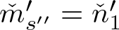 $\check m'_{s^{\prime\prime}}=\check n'_1$.
Next, using the notations in (3.55), we define
 \begin{equation}
S'=\sum_{j=1}^{s'}\frac1{\sigma'_j}Q'_j.
\end{equation}
Lemma 3.10. For each 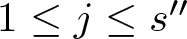 $1\le j\le s^{\prime\prime}$,
 \begin{equation}
\mathcal{Q}_j(L-AS'A)\mathcal{Q}_j=\frac12\sum_{k=\check m'_{j-1}+1}^{\check m'_j}\check\lambda^{\prime\prime}_k(0)\check P_k(0),
\end{equation}
with 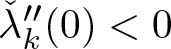 $\check\lambda^{\prime\prime}_k(0) \lt 0$,
 $\check m'_{j-1}+1\le k\le \check m'_j$.
In (3.61), by combining terms on the right-hand side with the same value of  $\check\lambda^{\prime\prime}_k(0)$, we obtain the spectral decomposition of the matrix on the left-hand side in the range of
 $\mathcal{Q}_j$. We thus write
 \begin{equation}
\mathcal{Q}_j(AS'A-L)\mathcal{Q}_j=\sum_{l=1}^{s_j}\beta_{jl}\mathcal{Q}_{jl},\qquad 1\le j\le s^{\prime\prime},
\end{equation}
where each  $\beta_{jl}$ is a distinct
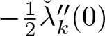 $-\frac12\check\lambda^{\prime\prime}_k(0)$,
 $\check m'_{j-1}+1\le k\le \check m'_j$,
 $\mathcal{Q}_{jl}$ is the sum of the corresponding
 $\check P_k(0)$’s that share the same value of
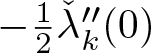 $-\frac12\check\lambda^{\prime\prime}_k(0)$, and
 $\sum_{l=1}^{s_j}\mathcal{Q}_{jl}=\sum_{k=\check m'_{j-1}+1}^{\check m'_j}\check P_k(0)=\mathcal{Q}_j$. We note that all
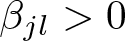 $\beta_{jl} \gt 0$.
We then collect all distinct pairs 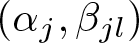 $(\alpha_j,\beta_{jl})$,
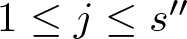 $1\le j\le s^{\prime\prime}$,
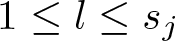 $1\le l\le s_j$. The total number of them is
 \begin{equation}
m'=\sum_{j=1}^{s^{\prime\prime}}s_j.
\end{equation}
We renames the triples  $(\alpha_j,\beta_{jl},\mathcal{Q}_{jl})$,
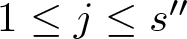 $1\le j\le s^{\prime\prime}$,
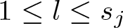 $1\le l\le s_j$, as
 $(\alpha_j,\beta_j, Q_{j,0}) $,
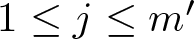 $1\le j\le m'$. Together with
 $m'$ defined in (3.63), these are parameters appearing in the third term on the right-hand side of (2.5). Clearly, from the construction described above, they are obtained through Steps 3 and 4 in Procedure 2.9. In particular, if all
 $\alpha_j$’s in (3.58) are simple, the process is reduced to Step 4
 $'$ in Appendix A.
We combine (3.52) and (3.54) to write
 \begin{equation}
E(z)=\sum_{j=1}^{\check n_1'}z^2\check\lambda_j(\frac1z)\check P_j(\frac1z)+\sum_{j=\check n_1'+1}^{n'}z^2\check\lambda_j(\frac1z)\check P_j(\frac1z).
\end{equation}
Applying Lemma 3.8, we have
 \begin{equation}
z^2\check\lambda_j(\frac1z)=\begin{cases}\check\lambda'_j(0)z+\frac12\check\lambda^{\prime\prime}_j(0)+\frac16\check\lambda'^{\prime\prime}_j(0)\frac1z+\cdots,\quad1\le j\le \check n'_1,\\
\check\lambda_j(0)z^2+\check\lambda'_j(0)z+\cdots,\quad \check n'_1+1\le j\le n',\end{cases}
\end{equation}
and for  $ \check n'_1+1\le j\le n'$, each
 $\check\lambda_j(0)$ is a positive eigenvalue of
 $B$.
Using (3.64) and (3.65), we extract leading terms of  $E(z)$ as
 $z\rightarrow\infty$ as follows. Let
 \begin{equation}
E^\#_0(z)=\sum_{j=1}^{\check n_1'}\Big[\check\lambda'_j(0)z+\frac12\check\lambda^{\prime\prime}_j(0)\Big]\check P_j(0).
\end{equation}
From (3.57)-(3.59), (3.61)-(3.63) and the definition of  $(\alpha_j,\beta_j,Q_{j,0})$,
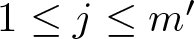 $1\le j\le m'$, we have
 \begin{equation}
\begin{aligned}
E^\#_0(z)&=z\sum_{j=1}^{\check n_1'}\check\lambda'_j(0)\check P_j(0)+\sum_{j=1}^{\check n_1'}\frac12\check\lambda^{\prime\prime}_j(0)\check P_j(0)\\
&=-z\sum_{j=1}^{s^{\prime\prime}}\alpha_j\mathcal{Q}_j+\sum_{j=1}^{s^{\prime\prime}}\sum_{k=\check m'_{j-1}+1}^{\check m'_j}\frac12\check\lambda^{\prime\prime}_k(0)\check P_k(0)\\
&=-z\sum_{j=1}^{s^{\prime\prime}}\alpha_j\sum_{l=1}^{s_j}\mathcal{Q}_{jl}-\sum_{j=1}^{s^{\prime\prime}}\sum_{l=1}^{s_j}\beta_{jl}\mathcal{Q}_{jl}\\
&=-\sum_{j=1}^{s^{\prime\prime}}\sum_{l=1}^{s_j}(\alpha_jz+\beta_{jl})\mathcal{Q}_{jl}\\
&=-\sum_{j=1}^{m'}(\alpha_jz+\beta_j)Q_{j,0}.
\end{aligned}
\end{equation}
Consider the semigroup generated by 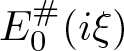 $E^\#_0(i\xi)$,
 \begin{equation}
\hat G_0^\#(\xi,t)=e^{tE^\#_0(i\xi)}=\sum_{j=1}^{m'}e^{(-\alpha_ji\xi-\beta_j)t}Q_{j,0}.
\end{equation}
Its inverse Fourier transform is
 \begin{equation*}
G_0^\#(x,t)=\sum_{j=1}^{m'}e^{-\beta_jt}\delta(x-\alpha_jt)Q_{j,0},
\end{equation*}
which is the third term on the right-hand side of (2.5) when  $l=0$. For
 $l\ge1$, the inverse transform of
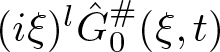 $(i\xi)^l\hat G_0^\#(\xi,t)$ gives the
 $l$th derivatives of the
 $\delta$-functions. To completely extract the singular part, i.e., the third term on the right-hand side of (2.5), we need an expansion of
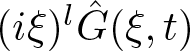 $(i\xi)^l\hat G(\xi,t)$ into higher-order terms as follows.
From (3.6), (3.64) and (3.65), for 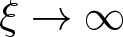 $\xi\rightarrow\infty$ we have
 \begin{equation*}
\begin{aligned}
(i\xi)^l\hat G(\xi,t)=&\sum_{j=1}^{\check n_1'}(i\xi)^le^{(i\xi)^2\check\lambda_j(1/i\xi)t}\check P_j(\frac1{i\xi})\\
&+\sum_{j=\check n_1'+1}^{n'}(i\xi)^le^{(i\xi)^2\check\lambda_j(1/i\xi)t}\check P_j(\frac1{i\xi})\\
=&\sum_{j=1}^{\check n_1'}e^{[i\xi\check\lambda_j'(0)+\frac12\check\lambda_j''(0)]t}(i\xi)^l\check P_j(\frac1{i\xi})\\
&+\sum_{j=1}^{\check n_1'}e^{[i\xi\check\lambda_j'(0)+\frac12\check\lambda_j''(0)]t}\Big\{e^{[(i\xi)^2\check\lambda_j(1/i\xi)-i\xi\check\lambda_j'(0)-\frac12\check\lambda_j''(0)]t}-1\Big\}(i\xi)^l\check P_j(\frac1{i\xi})\\
&+\sum_{j=\check n_1'+1}^{n'}O(1)(i\xi)^le^{[-\xi^2\check\lambda_j(0)+i\xi\check\lambda_j'(0)]t+O(1)t}.
\end{aligned}
\end{equation*}
We take Taylor expansion on the right-hand side to arrive at
 \begin{equation}
\begin{aligned}
(i\xi)^l\hat G(\xi,t)=&\sum_{j=1}^{\check n_1'}e^{[i\xi\check\lambda_j'(0)+\frac12\check\lambda_j''(0)]t}\Bigg[(i\xi)^l\check P_j(0)+\sum_{k=1}^l(i\xi)^{l-k}Q_{j,k}(t)\Bigg]\\
&+\sum_{j=1}^{\check n_1'}e^{[i\xi\check\lambda_j'(0)+\frac12\check\lambda_j''(0)]t}(i\xi)^{-1}Q_{j,l+1}(t)\\
&+\sum_{j=1}^{\check n_1'}e^{[i\xi\check\lambda_j'(0)+\frac12\check\lambda_j''(0)]t}\Big[O(1)(i\xi)^{-2}(1+t+\cdots+t^{l+1}+t^{l+2}e^{O(t/i\xi)})\Big]\\
&+\sum_{j=\check n_1'+1}^{n'}O(1)(i\xi)^le^{[-\xi^2\check\lambda_j(0)+i\xi\check\lambda_j'(0)]t+O(1)t},
\end{aligned}
\end{equation}
where we have used 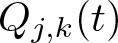 $Q_{j,k}(t)$ to denote an
 $n\times n$ matrix whose entries are polynomials in
 $t$ with degrees not larger than
 $k$. Similar to the derivation of
 $\hat G_0^\#$, see (3.66)-(3.68), we further simplify (3.69) to
 \begin{equation}
\begin{aligned}
(i\xi)^l\hat G(\xi,t)=&\sum_{j=1}^{m'}e^{(-\alpha_ji\xi-\beta_j)t}\sum_{k=0}^l(i\xi)^{l-k}Q_{j,k}(t)
+\sum_{j=1}^{m'}e^{(-\alpha_ji\xi-\beta_j)t}(i\xi)^{-1}Q_{j,l+1}(t)\\
&\quad+O(1)e^{-\beta t}\sum_{j=1}^{m'}e^{-\alpha_ji\xi t}(i\xi)^{-2}\\
&\quad+\sum_{j=\check n_1'+1}^{n'}O(1)(i\xi)^le^{[-\xi^2\check\lambda_j(0)+i\xi\check\lambda_j'(0)]t+O(1)t}\\
\equiv&\hat G_l^\#(\xi,t)+\hat R_{l1}^\#(\xi,t)+\hat R_{l2}^\#(\xi,t)+\hat R_{l3}^\#(\xi,t),
\end{aligned}
\end{equation}
where  $\beta=\frac12\min_{1\le j\le m'}\beta_j \gt 0$.
The leading term on the right-hand side of (3.70) is 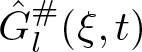 $\hat G_l^\#(\xi,t)$. Taking the inverse Fourier transform we have
 \begin{equation}
G_l^\#(x,t)=\sum_{j=1}^{m'}e^{-\beta_jt}\sum_{k=0}^l\delta^{(l-k)}
(x-\alpha_jt)Q_{j,k}(t).
\end{equation}
This is the third term on the right-hand side of (2.5).
In summary, in this section, we have constructed the leading terms of 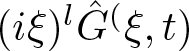 $(i\xi)^l\hat G^(\xi,t)$ for both small
 $\xi$ and large
 $\xi$, respectively. The former is
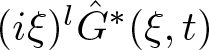 $(i\xi)^l\hat G^*(\xi,t)$, and the latter is
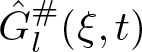 $\hat G_l^\#(\xi,t)$, see (3.48) and (3.70).
4. Estimation on inverse Fourier transforms
Based on the spectral analysis carried out in the Fourier space in Section 3, we now consider inverse transforms to obtain estimates for the Green’s function and its derivatives in the physical space. For convenience, we use  $C$ for a generic, positive constant in this section.
4.1. Proof of Theorem 2.3
With the key estimates (3.48) and (3.70), most of this part is parallel to the case of hyperbolic-parabolic conservation laws, discussed in [Reference Liu and Zeng14]. We include this part for completeness, with some updates or simplifications. Readers are referred to [Reference Liu and Zeng14] for more details.
With 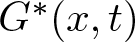 $G^*(x,t)$ and
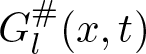 $G^\#_l(x,t)$ defined in (3.49) and (3.71), respectively, we set
 \begin{equation}
R^{(l)}(x,t)=\frac{\partial^l}{\partial x^l}G(x,t)-\frac{\partial^l}{\partial x^l}G^*(x,t)-G^\#_l(x,t).
\end{equation}
We only need to show that 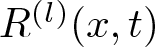 $R^{(l)}(x,t)$ is the second term on the right-hand side of (2.5) to prove Theorem 2.3.
For this, we use inverse Fourier transforms as follows,
 \begin{equation}
\begin{aligned}
R^{(l)}(x,t)=&\frac1{2\pi}\int_{-\infty}^{\infty}e^{ix\xi}\hat R^{(l)}(\xi,t)\,d\xi\\
=&\frac1{2\pi}\int_{-\infty}^{\infty}e^{ix\xi}[(i\xi)^l\hat G(\xi,t)-(i\xi)^l\hat G^*(\xi,t)-\hat G^\#_l(\xi,t)]\,d\xi\\
=&R^{(l)}_1(x,t)+R^{(l)}_2(x,t)+R^{(l)}_3(x,t),
\end{aligned}
\end{equation}
where
 \begin{equation}
\begin{aligned}
R^{(l)}_1(x,t)=&\frac1{2\pi}\int_{-\epsilon}^{\epsilon}e^{ix\xi}(i\xi)^l[\hat G(\xi,t)-\hat G^*(\xi,t)]\,d\xi,\\
R^{(l)}_2(x,t)=&\frac1{2\pi}\left(\int_{-\infty}^{-N}+\int_N^{\infty}\right)e^{ix\xi}[(i\xi)^l\hat G(\xi,t)-\hat G^\#_l(\xi,t)]\,d\xi,\\
R^{(l)}_3(x,t)=&\frac1{2\pi}\left(\int_{-N}^{-\epsilon}+\int_{\epsilon}^{N}\right)e^{ix\xi}(i\xi)^l\hat G(\xi,t)\,d\xi\\
-&\frac1{2\pi}\left(\int_{-\infty}^{-\epsilon}+\int_{\epsilon}^{\infty}\right)e^{ix\xi}(i\xi)^l\hat G^*(\xi,t)\,d\xi-\frac1{2\pi}\int_{-N}^{N}e^{ix\xi}
\hat G^\#_l(\xi,t)\,d\xi,
\end{aligned}
\end{equation}
and  $\epsilon \gt 0$ small and
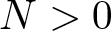 $N \gt 0$ large are to be chosen.
To estimate  $R^{(l)}_1$ we recall (3.6),(3.47) and (3.48) to have
 \begin{align}
R^{(l)}_1(x,t)=&\frac1{2\pi}\int_{-\epsilon}^{\epsilon}e^{ix\xi}(i\xi)^l[e^{tE(i\xi)}-e^{tE^*(i\xi)}]\,d\xi\nonumber\\
=&\frac1{2\pi}\int_{-\epsilon}^{\epsilon}e^{ix\xi}(i\xi)^l\left\{\sum_{j=1}^{n'_1}e^{\tilde\lambda_j(i\xi)t}\tilde P_j(i\xi)+\sum_{j=n'_1+1}^{n'}e^{\tilde\lambda_j(i\xi)t}\tilde P_j(i\xi)\right. \nonumber \\
&\left.-\sum_{j=1}^{n'_1}e^{[\tilde\lambda_j'(0)i\xi-\frac12\tilde\lambda^{\prime\prime}_j(0)\xi^2]t}\tilde P_j(0)\right\}\,d\xi\nonumber\\
\equiv&\sum_{j=1}^{n'_1}R^{(l)}_{1,j}(x,t)+\sum_{j=n'_1+1}^{n'}R^{(l)}_{1,j}(x,t),
\end{align}
where for 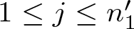 $1\le j\le n'_1$,
 \begin{equation}
R^{(l)}_{1,j}(x,t)=\frac1{2\pi}\int_{-\epsilon}^{\epsilon}e^{ix\xi}(i\xi)^l\{e^{\tilde\lambda_j(i\xi)t}\tilde P_j(i\xi)-e^{[\tilde\lambda_j'(0)i\xi-\frac12\tilde\lambda^{\prime\prime}_j(0)\xi^2]t}\tilde P_j(0)\}\,d\xi,
\end{equation}
and for  $n'_1+1\le j\le n'$,
 \begin{equation}
R^{(l)}_{1,j}(x,t)=\frac1{2\pi}\int_{-\epsilon}^{\epsilon}e^{ix\xi}(i\xi)^le^{\tilde\lambda_j(i\xi)t}\tilde P_j(i\xi)\,d\xi.
\end{equation}
We note that  $\tilde\lambda_j(z)$ and
 $\tilde P_j(z)$ are holomorphic at the origin. By taking
 $\epsilon$ small,
 $\tilde\lambda_j(z)$ and
 $\tilde P_j(z)$ are holomorphic in a
 $2\epsilon$-neighbourhood of the origin, which allows us to apply the Cauchy integral theorem there. For this, we regard
 $\xi$ as a complex variable. For our convenience, we also introduce the path
 \begin{equation}
\begin{aligned}
\sigma(a,b,c)=&\{\xi\,|\,{\rm Re}\,\xi=a, {\rm Im}\, \xi\,\mbox{is from}\ 0\ \mbox{to}\ c\}\cup\{\xi\,|\,{\rm Im}\,\xi=c, {\rm Re}\, \xi\,\mbox{is from}\ a\ \mbox{to}\ b\}\\
&\cup\{\xi\,|\,{\rm Re}\,\xi=b, {\rm Im}\, \xi\,\mbox{is from}\ c\ \mbox{to}\ 0\}
\end{aligned}
\end{equation}
for 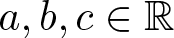 $a,b,c\in\mathbb{R}$, see figure 1.
Integration path for inverse Fourier transforms.

We first estimate  $R^{(l)}_{1,j}$ for
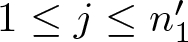 $1\le j\le n'_1$, see (4.5). If
 $\xi$ is in the
 $2\epsilon$-neighbourhood of the origin, we use Taylor expansion to write
 \begin{equation}
\begin{aligned}
&e^{\tilde\lambda_j(i\xi)t}\tilde P_j(i\xi)-e^{[\tilde\lambda_j'(0)i\xi-\frac12\tilde\lambda^{\prime\prime}_j(0)\xi^2]t}\tilde P_j(0)\\
=&i\xi e^{[\tilde\lambda_j'(0)i\xi-\frac12\tilde\lambda^{\prime\prime}_j(0)\xi^2]t}[O(1)+O(1)\xi^2te^{O(1)(i\xi)^3t}]\\
=&i\xi e^{[-\lambda_k^{(r)}i\xi-\mu_k\xi^2]t}[O(1)+O(1)\xi^2te^{O(1)(i\xi)^3t}],
\end{aligned}
\end{equation}
where we have applied (3.48), and  $k$ is an integer determined by
 $j$,
 $1\le k\le m$. Now we consider two cases.
Case 1 is for  $|x-\lambda_k^{(r)}t|/(2\mu_kt)\le\frac12\epsilon$. In this case, we replace
 $[-\epsilon,\epsilon]$ by
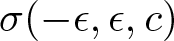 $\sigma(-\epsilon,\epsilon,c)$ in (4.5), with
 $c=(x-\lambda_k^{(r)}t)/(2\mu_kt)$. Note that
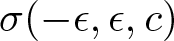 $\sigma(-\epsilon,\epsilon,c)$ is in the
 $2\epsilon$-neighbourhood of the origin. Applying (4.8), we reduce (4.5) to
 \begin{equation}
R^{(l)}_{1,j}(x,t)=\frac1{2\pi}\int_{\sigma(-\epsilon,\epsilon,c)}(i\xi)^{l+1}e^{i\xi(x-\lambda_k^{(r)}t)-\mu_k\xi^2t}[O(1)+O(1)\xi^2te^{O(1)(i\xi)^3t}]\,d\xi.
\end{equation}
Along the middle part of 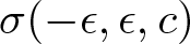 $\sigma(-\epsilon,\epsilon,c)$, with the specific choice of
 $c$, we have
 $\xi=\zeta+i(x-\lambda_k^{(r)}t)/(2\mu_kt)$, and hence
 \begin{equation}
i\xi(x-\lambda_k^{(r)}t)=i\zeta(x-\lambda_k^{(r)}t)-\frac{(x-\lambda_k^{(r)}t)^2}{2\mu_kt},\qquad-\epsilon\le\zeta\le\epsilon.
\end{equation}
Similarly, along the first and the third parts of 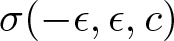 $\sigma(-\epsilon,\epsilon,c)$,
 $\xi=\mp\epsilon+i\eta$, and
 \begin{equation}
i\xi(x-\lambda_k^{(r)}t)=\mp i\epsilon(x-\lambda_k^{(r)}t)-(x-\lambda_k^{(r)}t)\eta,\qquad \eta\ \mbox{between 0 and}\ c.
\end{equation}
We note that in (4.11), 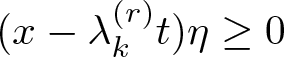 $(x-\lambda_k^{(r)}t)\eta\ge0$.
Substituting (4.10) and (4.11) into (4.9) and taking  $\epsilon \gt 0$ small, we have
 \begin{equation*}
\begin{aligned}
|R^{(l)}_{1,j}(x,t)|\le &C\int_{-\epsilon}^{\epsilon}\bigg[|\zeta|^{l+1}+\bigg(\frac{|x-\lambda_k^{(r)}t|}{2\mu_kt}\bigg)^{l+1}\bigg]e^{-\frac{(x-\lambda_k^{(r)}t)^2}{4\mu_k't}-\frac{\mu_k}2\zeta^2t}\\
&\times\bigg[1+\zeta^2t+\frac{(x-\lambda_k^{(r)}t)^2}t\bigg]\,d\zeta+C\epsilon^{l+2}e^{-\frac34\epsilon^2\mu_kt}[1+\epsilon^2te^{C\epsilon^3t}],
\end{aligned}
\end{equation*}
where 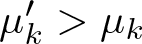 $\mu'_k \gt \mu_k$ is a generic constant. Thus, by adjusting
 $\mu'_k$ slightly larger, we further have
 \begin{align}
|R^{(l)}_{1,j}(x,t)|\le C\int_{-\epsilon}^{\epsilon}\bigg[|\zeta|^{l+1}+\bigg(\frac{|x-\lambda_k^{(r)}t|}{2\mu_kt}\bigg)^{l+1}\bigg]e^{-\frac{(x-\lambda_k^{(r)}t)^2}{4\mu_k't}-\frac{\mu_k}4\zeta^2t}\,d\zeta
+C\epsilon^{l+2}e^{-\frac12\epsilon^2\mu_kt}.
\end{align}
Now we consider  $t \gt rless1$. If
 $t\ge1$, we use
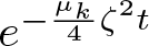 $e^{-\frac{\mu_k}4\zeta^2t}$ to absorb
 $\zeta^2t$ and
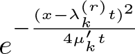 $e^{-\frac{(x-\lambda_k^{(r)}t)^2}{4\mu_k't}}$ to absorb
 $(x-\lambda_k^{(r)}t)^2/(4\mu_k^2t)$. Then we evaluate the integral in (4.12) to arrive at
 \begin{equation*}
\begin{aligned}
|R^{(l)}_{1,j}(x,t)|\le &C\int_{-\epsilon}^{\epsilon}t^{-\frac{l+1}2}e^{-\frac{(x-\lambda_k^{(r)}t)^2}{4\mu_k't}-\frac{\mu_k}8\zeta^2t}\,d\zeta+Ce^{-t/C}\\
\le &Ct^{-\frac{l+2}2}e^{-\frac{(x-\lambda_k^{(r)}t)^2}{4\mu_k't}}+Ce^{-t/C}\le C(t+1)^{-\frac{l+2}2}e^{-\frac{(x-\lambda_k^{(r)}t)^2}{4\mu_k't}}+Ce^{-t/C}.
\end{aligned}
\end{equation*}
If  $t\le1$, (4.12) gives us
 \begin{equation*}
\begin{aligned}
|R^{(l)}_{1,j}(x,t)|\le &C\epsilon^{l+2}e^{-\frac{(x-\lambda_k^{(r)}t)^2}{4\mu_k't}}+C\epsilon^{l+2}e^{-\frac12\epsilon^2\mu_kt}\\
\le&C(t+1)^{-\frac{l+2}2}e^{-\frac{(x-\lambda_k^{(r)}t)^2}{4\mu_k't}}+Ce^{-t/C}.
\end{aligned}
\end{equation*}
Therefore, we obtain a key estimate in Case 1: for  $t \gt 0$,
 $x\in\mathbb{R}$,
 \begin{equation}
|R^{(l)}_{1,j}(x,t)|\le C(t+1)^{-\frac{l+2}2}e^{-\frac{(x-\lambda_k^{(r)}t)^2}{4\mu_k't}}+Ce^{-t/C},\qquad1\le j\le n'_1.
\end{equation}
Case 2 is for  $|x-\lambda_k^{(r)}t|/(2\mu_kt)\ge\frac12\epsilon$. In this case, we replace
 $[-\epsilon,\epsilon]$ by
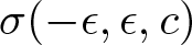 $\sigma(-\epsilon,\epsilon,c)$ in (4.5), with
 $c=\frac{\epsilon}2{\rm sign}(x-\lambda_k^{(r)}t)$. Since
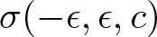 $\sigma(-\epsilon,\epsilon,c)$ is in the
 $2\epsilon$-neighbourhood of the origin, we still have (4.9) for
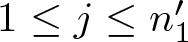 $1\le j\le n'_1$. Similar to the derivation of (4.12),
 \begin{equation}
\begin{aligned}
|R^{(l)}_{1,j}(x,t)|\le &\frac1{2\pi}\int_{-\epsilon}^{\epsilon}\bigg[|\zeta|+\big(\frac{\epsilon}2\big)\bigg]^{l+1}e^{-\frac{\epsilon}2|x-\lambda_k^{(r)}t|-\mu_k\zeta^2t+\frac{\epsilon^2}4\mu_kt}\\
&\left[O(1)+O(1)\epsilon^2te^{C\epsilon^3t}\right]\,d\zeta + \frac1{\pi}\int_0^{\frac{\epsilon}2}(\eta+\epsilon)^{l+1}e^{-\eta|x-\lambda_k^{(r)}t|-\epsilon^2\mu_kt+\eta^2\mu_kt}\\
&\left[O(1)+O(1)\epsilon^2te^{C\epsilon^3t}\right]\,d\eta\\
\le &C\int_{-\epsilon}^{\epsilon}\epsilon^{l+1}e^{-\frac14\epsilon^2\mu_kt-\mu_k\zeta^2t}(1+\epsilon^2te^{C\epsilon^3t})\,d\zeta+Ce^{-t/C}\le Ce^{-t/C}.
\end{aligned}
\end{equation}
Combining (4.13) and (4.14), for 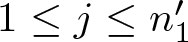 $1\le j\le n'_1$ we have
 \begin{equation}
|R^{(l)}_{1,j}(x,t)|\le C(t+1)^{-\frac{l+2}2}e^{-\frac{(x-\lambda_k^{(r)}t)^2}{4\mu_k't}}+Ce^{-t/C},\qquad x\in\mathbb{R},\quad t \gt 0.
\end{equation}
Now we estimate  $R^{(l)}_{1,j}$ for
 $n'_1+1\le j\le n'$. From (4.6), we have
 \begin{equation}
R^{(l)}_{1,j}(x,t)=\frac1{2\pi}\int_{-\epsilon}^{\epsilon}(i\xi)^{l}e^{ix\xi+\tilde\lambda_j(0)t+O(i\xi)t}O(1)\,d\xi.
\end{equation}
Noting that for  $n'_1+1\le j\le n'$,
 $\tilde\lambda_j(z)$ is in group two, see the definition of
 $n'_1$ beneath Lemma 3.4. Then by Lemma 3.3, each
 $\tilde\lambda_j(0)$ is some
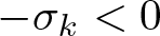 $-\sigma_k \lt 0$, a negative eigenvalue of
 $L$. Therefore, (4.16) gives us
 \begin{equation}
|R^{(l)}_{1,j}(x,t)|\le Ce^{-t/C},\qquad t\ge0,
\end{equation}
for  $n'_1+1\le j\le n'$.
Substituting (4.15) and (4.17) into (4.4), we arrive at
 \begin{equation}
|R^{(l)}_{1}(x,t)|\le C\sum_{k=1}^m(t+1)^{-\frac{l+2}2}e^{-\frac{(x-\lambda_k^{(r)}t)^2}{4\mu_k't}}+Ce^{-t/C},\qquad x\in\mathbb{R},\quad t \gt 0.
\end{equation}
Next, we consider  $R^{(l)}_{2}$ in (4.3). Substituting (3.70) into (4.3) gives us
 \begin{equation}
\begin{aligned}
R^{(l)}_2(x,t)&=\frac1{2\pi}\left(\int_{-\infty}^{-N}+\int_N^{\infty}\right)e^{ix\xi}[\hat R_{l1}^{\#}(\xi,t)+\hat R_{l2}^{\#}(\xi,t)+\hat R_{l3}^\#(\xi,t)]\,d\xi\\
&\equiv R^{(l)}_{21}(x,t)+R^{(l)}_{22}(x,t)+R^{(l)}_{23}(x,t),
\end{aligned}
\end{equation}
where
 \begin{equation*}
\begin{aligned}
R^{(l)}_{21}(x,t)&=\frac1{2\pi}\left(\int_{-\infty}^{-N}+\int_N^{\infty}\right)e^{ix\xi}\hat R_{l1}^{\#}(\xi,t)\,d\xi\\
&=\frac1{2\pi}\left(\int_{-\infty}^{-N}+\int_N^{\infty}\right)\sum_{j=1}^{m'}e^{i(x-\alpha_jt)\xi-\beta_jt}(i\xi)^{-1}\,d\xi Q_{j,l+1}(t),\\
R^{(l)}_{22}(x,t)&=\frac1{2\pi}\left(\int_{-\infty}^{-N}+\int_N^{\infty}\right)e^{ix\xi}\hat R_{l2}^{\#}(\xi,t)\,d\xi\\
&=e^{-\beta t}\left(\int_{-\infty}^{-N}+\int_N^{\infty}\right)O(1)\sum_{j=1}^{m'}e^{i(x-\alpha_jt)\xi}(i\xi)^{-2}\,d\xi,\\
R^{(l)}_{23}(x,t)&=\frac1{2\pi}\left(\int_{-\infty}^{-N}+\int_N^{\infty}\right)e^{ix\xi}\hat R_{l3}^{\#}(\xi,t)\,d\xi\\
&=\left(\int_{-\infty}^{-N}+\int_N^{\infty}\right)\sum_{j=\check n_1'+1}^{n'}O(1)(i\xi)^le^{-\xi^2\check\lambda_j(0)t+i(x+\check\lambda_j'(0)t)\xi +O(1)t}\,d\xi,
\end{aligned}
\end{equation*}
where 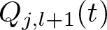 $Q_{j,l+1}(t)$ are
 $n\times n$ matrices whose entries are polynomials in
 $t$ with degrees not larger than
 $l+1$;
 $\beta \gt 0$ is a constant; and
 $\check\lambda_j(0)$ are positive eigenvalues of
 $B$ for
 $\check n'_1+1\le j\le n'$.
Noting the integral in  $R^{(l)}_{21}$ is for the principal value and by properties of the sinc function, we have
 \begin{equation*}
|R^{(l)}_{21}(x,t)|\le\frac1{2\pi}\sum_{j=1}^{m'}e^{-\beta_jt}\left|\left(\int_{-\infty}^{-N}+\int_N^{\infty}\right)\frac{\sin((x-\alpha_jt)\xi)}{\xi}\,d\xi\right| |Q_{j,l+1}(t)|\le Ce^{-t/C}.
\end{equation*}
It is also straightforward to have
 \begin{equation*}
|R^{(l)}_{22}(x,t)|\le Ce^{-t/C},\qquad|R^{(l)}_{23}(x,t)|\le Ct^{-\frac{l+1}2}e^{-t/C}.
\end{equation*}
Thus,
 \begin{equation}
|R^{(l)}_{2}(x,t)|\le Ct^{-\frac{l+1}2}e^{-t/C}+Ce^{-t/C}.
\end{equation}
To consider  $R^{(l)}_3$ in (4.3), we write
 \begin{equation}
R^{(l)}_3(x,t)=R^{(l)}_{31}(x,t)+R^{(l)}_{32}(x,t)+R^{(l)}_{33}(x,t),
\end{equation}
where
 \begin{equation}
\begin{aligned}
R^{(l)}_{31}(x,t)&=\frac1{2\pi}\left(\int_{-N}^{-\epsilon}+\int_{\epsilon}^N\right)e^{ix\xi}(i\xi)^l\hat G(\xi,t)\,d\xi,\\
R^{(l)}_{32}(x,t)&=-\frac1{2\pi}\left(\int_{-\infty}^{-\epsilon}+\int_{\epsilon}^{\infty}\right)e^{ix\xi}(i\xi)^l\hat G^*(\xi,t)\,d\xi,\\
R^{(l)}_{33}(x,t)&=-\frac1{2\pi}\int_{-N}^{N}e^{ix\xi}\hat G_l^{\#}(\xi,t)\,d\xi.
\end{aligned}
\end{equation}
We also cite Lemma 3.2 in [Reference Zeng34], which modifies a result from [Reference Kawashima9].
Lemma 4.1. There exist positive constants  $C$ and
 $c$ such that
 \begin{equation}
|e^{tE(i\xi)}|\le Ce^{-\frac{c\xi^2t}{1+\xi^2}},\qquad\xi\in \mathbb{R}, \quad t\ge0.
\end{equation}
Applying (3.6) and (4.23) to (4.22)1, we have
 \begin{equation}
\begin{aligned}
|R^{(l)}_{31}(x,t)|&=\frac1{2\pi}\left|\left(\int_{-N}^{-\epsilon}+\int_{\epsilon}^N\right)e^{ix\xi}(i\xi)^le^{tE(i\xi)}\,d\xi\right|\\
&\le C\left(\int_{-N}^{-\epsilon}+\int_{\epsilon}^N\right)|\xi|^le^{-\frac{c\xi^2t}{1+\xi^2}}\,d\xi\le Ce^{-t/C}.
\end{aligned}
\end{equation}
Applying (3.48) and (3.70) to (4.22)2 and (4.22)3, respectively, we have
 \begin{equation}
\begin{aligned}
|R^{(l)}_{32}(x,t)|&\le C\left(\int_{-\infty}^{-\epsilon}+\int_{\epsilon}^{\infty}\right)|\xi|^l\sum_{j=1}^me^{-\mu_j\xi^2t}\,d\xi\le Ct^{-\frac{l+1}2}e^{-t/C},\\
|R^{(l)}_{33}(x,t)|&\le C\int_{-N}^{N}\sum_{j=1}^{m'}e^{-\beta_jt}\sum_{k=0}^l|\xi|^{l-k}|Q_{j,k}(t)|\,d\xi\le Ce^{-t/C}.
\end{aligned}
\end{equation}
Thus, (4.21) gives us
 \begin{equation}
|R^{(l)}_3(x,t)|\le Ct^{-\frac{l+1}2}e^{-t/C}+Ce^{-t/C}.
\end{equation}
We now substitute (4.18), (4.20) and (4.26) into (4.2) to arrive at
 \begin{equation}
|R^{(l)}(x,t)|\le C\sum_{k=1}^m(t+1)^{-\frac{l+2}2}e^{-\frac{(x-\lambda_k^{(r)}t)^2}{4\mu_k't}}+Ce^{-t/C}+Ct^{-\frac{l+1}2}e^{-t/C}.
\end{equation}
Here, (4.27) holds for 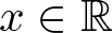 $x\in\mathbb{R}$ and
 $t \gt 0$.
Next, we consider large  $x/t$. Suppose
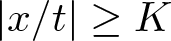 $|x/t|\ge K$ for a large positive constant
 $K$. We consider
 \begin{equation}
\tilde R^{(l)}(x,t)\equiv\frac{\partial^l}{\partial x^l}G(x,t)-G^{\#}_l(x,t)=\frac1{2\pi}\int_{-\infty}^{\infty}e^{ix\xi}[(i\xi)^l\hat G(\xi,t)-\hat G^{\#}_l(\xi,t)]\,d\xi.
\end{equation}
 \begin{equation*}
\tilde R^{(l)}(x,t)=\frac1{2\pi}\int_{-\infty}^{\infty}e^{ix\xi}[(i\xi)^le^{tE(i\xi)}-\sum_{j=1}^{m'}e^{(-\alpha_ji\xi-\beta_j)t}\sum_{k=0}^l(i\xi)^{l-k}Q_{j,k}(t)]\,d\xi.
\end{equation*}
Noting that the integrand on the right-hand side is an entire function, we apply the Cauchy integral theorem and move the integration path to  $\sigma=\sigma(-N,N,\nu x/t)$, where
 $\nu \gt 0$ is a constant to be determined and
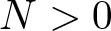 $N \gt 0$ is large. For large
 $N$ and
 $K$ we apply (3.70) on
 $\sigma$. That is
 \begin{equation}
\tilde R^{(l)}(x,t)=\frac1{2\pi}\int_{\sigma}e^{ix\xi}[\hat R_{l1}^\#(\xi,t)+\hat R_{l2}^\#(\xi,t)+\hat R_{l3}^\#(\xi,t)]\,d\xi,
\end{equation}
with 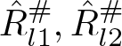 $\hat R_{l1}^\#,\hat R_{l2}^\#$ and
 $\hat R_{l3}^\#$ defined in (3.70). By the formulation of
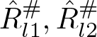 $\hat R_{l1}^\#,\hat R_{l2}^\#$ and
 $\hat R_{l3}^\#$, it is clear that as
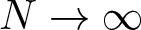 $N\rightarrow\infty$, the integrals on the line segments
 $\{\pm N+i\eta\,|\,\eta\ \mbox{between 0 and}\ \nu x/t\}$ approach to zero for fixed
 $x$ and
 $t \gt 0$. Therefore, we further reduce (4.29) to
 \begin{equation}
\begin{aligned}
\tilde R^{(l)}(x,t)&=\frac1{2\pi}\int_{{\rm Im}\xi=\frac{\nu x}t}e^{ix\xi}[\hat R_{l1}^\#(\xi,t)+\hat R_{l2}^\#(\xi,t)+\hat R_{l3}^\#(\xi,t)]\,d\xi\\
&=\tilde R^{(l)}_1(x,t)+\tilde R^{(l)}_2(x,t)+\tilde R^{(l)}_3(x,t),
\end{aligned}
\end{equation}
where
 \begin{equation}
\tilde R^{(l)}_j(x,t)=\frac1{2\pi}\int_{{\rm Im}\xi=\frac{\nu x}t}e^{ix\xi}\hat R_{lj}^\#(\xi,t)\,d\xi,\qquad1\le j\le3.
\end{equation}
From (3.70), we have
 \begin{equation}
|\tilde R^{(l)}_1(x,t)|\le\frac1{2\pi}\sum_{j=1}^{m'}e^{-\frac{\nu x}{t}(x-\alpha_jt)-\beta_jt}\left|\int_{-\infty}^{\infty}\frac{e^{i\zeta(x-\alpha_jt)}}{i\zeta-\frac{\nu x}t}\,d\zeta\right| |Q_{j,l+1}(t)|.
\end{equation}
By algebraic manipulation, we have
 \begin{equation*}
\frac1{i\zeta-\frac{\nu x}t}=\frac1{i\zeta}-\frac{\frac{\nu x}t}{\zeta^2+(\frac{\nu x}t)^2}-\frac1{i\zeta}\frac{(\frac{\nu x}t)^2}{\zeta^2+(\frac{\nu x}t)^2}.
\end{equation*}
Noting that the integral is for the principal value, we have
 \begin{align*}
\int_{-\infty}^{\infty}\frac{e^{i\zeta(x-\alpha_jt)}}{i\zeta-\frac{\nu x}t}\,d\zeta&=\int_{-\infty}^{\infty}\frac{\sin(\zeta(x-\alpha_jt))}{\zeta}\left[1-\frac{(\frac{\nu x}t)^2}{\zeta^2+(\frac{\nu x}t)^2}\right]\,d\zeta \nonumber \\
&-\int_{-\infty}^{\infty}\frac{\cos(\zeta(x-\alpha_jt))}{\zeta^2+(\frac{\nu x}t)^2}\frac{\nu x}t\,d\zeta.
\end{align*}
Thus,
 \begin{equation}
\begin{aligned}
\left|\int_{-\infty}^{\infty}\frac{e^{i\zeta(x-\alpha_jt)}}{i\zeta-\frac{\nu x}t}\,d\zeta\right|\le&\pi+ \int_{|\zeta| \lt |x-\alpha_jt|^{-1}}\left|\frac{\sin(\zeta(x-\alpha_jt))}{\zeta}\right|\,d\zeta\\
&+\int_{|\zeta| \gt |x-\alpha_jt|^{-1}}\frac{(\frac{\nu x}t)^2}{|\zeta|[\zeta^2+(\frac{\nu x}t)^2]}\,d\zeta
+\int_{-\infty}^{\infty}\frac{|\frac{\nu x}t|}{\zeta^2+(\frac{\nu x}t)^2}\,d\zeta\\
\le&C+\ln\left[1+\left(\frac{\nu x}t\right)^2|x-\alpha_jt|^2\right].
\end{aligned}
\end{equation}
Substituting (4.33) into (4.32) and taking  $K\ge3\max_{1\le j\le m'}|\alpha_j|$ give us
 \begin{equation}
|\tilde R^{(l)}_1(x,t)|\le Ce^{-\frac{\nu x^2}{2t}-t/C}.
\end{equation}
From (3.70) and (4.31), and by taking 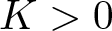 $K \gt 0$ large and
 $\nu \gt 0$ such that
 $\nu\max_{\check n_1'+1\le j\le n'}\check\lambda_j(0)\le\frac12$, we also have
 \begin{equation}
\begin{aligned}
|\tilde R^{(l)}_2(x,t)|\le& Ce^{-\frac{\nu x^2}{2t}-t/C}\int_{-\infty}^{\infty}\frac{d\zeta}{\zeta^2+(\frac{\nu x}t)^2}\le
Ce^{-\frac{\nu x^2}{2t}-t/C},\\
|\tilde R^{(l)}_3(x,t)|\le& Ce^{-\frac{\nu x^2}{2t}+C|x|}\sum_{j=\check n_1'+1}^{n'}\int_{-\infty}^{\infty}\left(|\zeta|^l+\left|\frac{\nu x}t\right|^l\right)e^{-\check\lambda_j(0)\zeta^2t}\,d\zeta\\
\le &Ce^{-\frac{\nu x^2}{2t}+C|x|}\left(t^{-\frac{l+1}2}+t^{-\frac12}\left|\frac{\nu x}t\right|^l\right)\\
\le &Ce^{-\frac{\nu x^2}{2t}+C\frac{x^2}{Kt}}\left(t^{-\frac{l+1}2}+t^{-\frac12}\left|\frac{\nu x}t\right|^l\right)\\
\le &Ce^{-\frac{\nu x^2}{4t}}t^{-\frac{l+1}2}.
\end{aligned}
\end{equation}
Combining (4.30), (4.34), and (4.35), we arrive at
 \begin{equation}
|\tilde R^{(l)}(x,t)|\le Ce^{-\frac{\nu x^2}{4t}}(e^{-t/C}+t^{-\frac{l+1}2})
\end{equation}
for 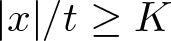 $|x|/t\ge K$, with
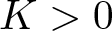 $K \gt 0$ large.
We now finish the proof of Theorem 2.3 by showing that 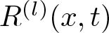 $R^{(l)}(x,t)$ is the second term on the right-hand side of (2.5). Fix a large
 $K \gt 2\max_{1\le j\le m}|\lambda^{(r)}_j|$ such that (4.36) holds. Then for
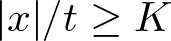 $|x|/t\ge K$,
 \begin{equation}
e^{-\frac{\nu x^2}{8t}}\le e^{-\frac{(x-\lambda^{(r)}_1t)^2}{Ct}}e^{\frac{(1+|\lambda^{(r)}_1|/K)^2x^2}{Ct}-\frac{\nu x^2}{8t}}\le e^{-\frac{(x-\lambda^{(r)}_1t)^2}{Ct}}
\end{equation}
by choosing a large  $C \gt 0$. Thus, (4.36) is reduced to
 \begin{equation}
|\tilde R^{(l)}(x,t)|\le C(t+1)^{-\frac12}t^{-\frac{l+1}2}e^{-\frac{(x-\lambda^{(r)}_1t)^2}{Ct}}.
\end{equation}
From (4.1), (4.28), (4.38), (3.49), and (2.4), we have
 \begin{equation*}
\begin{aligned}
|R^{(l)}(x,t)|\le&|\tilde R^{(l)}(x,t)|+|\frac{\partial^l}{\partial x^l}G^*(x,t)|\\
\le&C(t+1)^{-\frac12}t^{-\frac{l+1}2}e^{-\frac{(x-\lambda^{(r)}_1t)^2}{Ct}}+\sum_{j=1}^m|\frac{\partial^l}{\partial x^l}H(x,t;\lambda^{(r)}_j,\mu_j)P_j|\\
\le&C(t+1)^{-\frac12}t^{-\frac{l+1}2}\sum_{j=1}^me^{-\frac{(x-\lambda^{(r)}_jt)^2}{Ct}}.
\end{aligned}
\end{equation*}
This gives us the second term on the right-hand side of (2.5).
For 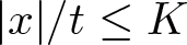 $|x|/t\le K$, on the other hand, we recall (4.27). Note that for a fixed
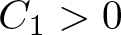 $C_1 \gt 0$,
 \begin{equation}
\begin{aligned}
e^{-t/C_1}\le&\, e^{-\frac{(x-\lambda^{(r)}_1t)^2}{Ct}}e^{\frac{(|x|/t+|\lambda^{(r)}_1|)^2t}{C}-\frac t{C_1}}\\
\le&\, e^{-\frac{(x-\lambda^{(r)}_1t)^2}{Ct}}e^{\frac{(K+|\lambda^{(r)}_1|)^2t}{C}-\frac t{C_1}}\le e^{-\frac{(x-\lambda^{(r)}_1t)^2}{Ct}}
\end{aligned}
\end{equation}
by choosing  $C \gt 0$ large. We thus reduce (4.27) to
 \begin{equation*}
|R^{(l)}(x,t)|\le C\sum_{k=1}^m(t+1)^{-\frac12}t^{-\frac{l+1}2}e^{-\frac{(x-\lambda_k^{(r)}t)^2}{Ct}}
\end{equation*}
for 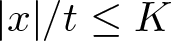 $|x|/t\le K$. This also gives us the second term on the right-hand side of (2.5). Now we have finished the proof of Theorem 2.3.
4.2. Justification of Remark 2.4
Now we justify Remark 2.4 to remove the singularity  $t^{-\frac{l+1}2}$ in the special case
 $B=0$. For this, we modify
 $R^{(l)}$ in (4.1) and set
 \begin{equation}
\bar R^{(l)}(x,t)=\frac{\partial^l}{\partial x^l}G(x,t)-\frac N{\pi}\operatorname{sinc}(Nx)\ast\frac{\partial^l}{\partial x^l}G^*(x,t)-G^{\#}_l(x,t).
\end{equation}
Noting that the Fourier transform of 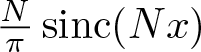 $\frac N{\pi}\operatorname{sinc}(Nx)$ is the characteristic function
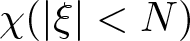 $\chi(|\xi| \lt N)$, we let
 \begin{equation}
\bar R^{(l)}(x,t)=R^{(l)}_1(x,t)+R^{(l)}_2(x,t)+\bar R^{(l)}_3(x,t),
\end{equation}
where  $R^{(l)}_1$ and
 $R^{(l)}_2$ are defined in (4.3), and
 \begin{equation*}
\begin{aligned}
\bar R^{(l)}_3(x,t)=&\frac1{2\pi}\left(\int_{-N}^{-\epsilon}+\int_{\epsilon}^{N}\right)e^{ix\xi}(i\xi)^l\hat G(\xi,t)\,d\xi\\
-&\frac1{2\pi}\left(\int_{-N}^{-\epsilon}+\int_{\epsilon}^{N}\right)e^{ix\xi}(i\xi)^l\hat G^*(\xi,t)\,d\xi-\frac1{2\pi}\int_{-N}^{N}e^{ix\xi}
\hat G^\#_l(\xi,t)]\,d\xi.
\end{aligned}
\end{equation*}
Comparing with  $R^{(l)}_3$ in (4.3), we have
 \begin{equation}
\bar R^{(l)}_3(x,t)=R^{(l)}_{31}(x,t)+\bar R^{(l)}_{32}(x,t)+R^{(l)}_{33}(x,t),
\end{equation}
where  $R^{(l)}_{31}$ and
 $R^{(l)}_{33}$ are defined in (4.22), and
 \begin{equation}
\bar R^{(l)}_{32}(x,t)=-\frac1{2\pi}\left(\int_{-N}^{-\epsilon}+\int_{\epsilon}^{N}\right)e^{ix\xi}(i\xi)^l\hat G^*(\xi,t)\,d\xi.
\end{equation}
Next, we note that when  $B=0$,
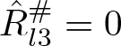 $\hat R_{l3}^\#=0$ in (3.70), see Lemma 3.8. This implies
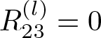 $R^{(l)}_{23}=0$ in (4.19), and hence we modify (4.20) to have
 \begin{equation}
|R^{(l)}_2(x,t)|\le Ce^{-t/C}.
\end{equation}
From (4.43) and (3.48) it is straightforward to have
 \begin{equation*}
|\bar R^{(l)}_{32}(x,t)|\le C\left(\int_{-N}^{-\epsilon}+\int_{\epsilon}^{N}\right)|\xi|^l\sum_{j=1}^me^{-\mu_j\xi^2t}\,d\xi\le Ce^{-t/C}.
\end{equation*}
Thus, comparing  $\bar R^{(l)}_3$ in (4.42) with
 $R^{(l)}_3$ in (4.21), we modify (4.26) to have
 \begin{equation}
|\bar R^{(l)}_3(x,t)|\le Ce^{-t/C}.
\end{equation}
Combining (4.41), (4.18), (4.44), and (4.45) gives us
 \begin{equation*}
|\bar R^{(l)}(x,t)|\le C\sum_{k=1}^m(t+1)^{-\frac{l+2}2}e^{-\frac{(x-\lambda^{(r)}_kt)^2}{4\mu'_kt}}+Ce^{-t/C}.
\end{equation*}
For 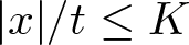 $|x|/t\le K$ we apply (4.39) to absorb the last term on the right -hand side and have
 \begin{equation}
|\bar R^{(l)}(x,t)|\le C\sum_{k=1}^m(t+1)^{-\frac{l+2}2}e^{-\frac{(x-\lambda^{(r)}_kt)^2}{Ct}}.
\end{equation}
Noting the definition of  $G^*$ and
 $G^{\#}_l$ in (3.49) and (3.71), respectively, (2.6) is justified for the case
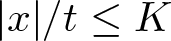 $|x|/t\le K$ by combining (4.40) and (4.46).
For the case 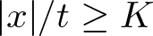 $|x|/t\ge K$ we recall
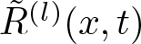 $\tilde R^{(l)}(x,t)$ defined in (4.28). Since
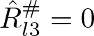 $\hat R_{l3}^\#=0$ for
 $B=0$,
 $\tilde R^{(l)}_3$ in (4.30) is zero. Thus, (4.36) becomes
 \begin{equation*}
|\tilde R^{(l)}(x,t)|\le Ce^{-\frac{\nu x^2}{2t}-t/C}.
\end{equation*}
Applying (4.37), we write
 \begin{equation}
|\tilde R^{(l)}(x,t)|\le C(t+1)^{-\frac{l+2}2}e^{-\frac{(x-\lambda^{(r)}_1t)^2}{Ct}}.
\end{equation}
Combining (4.28) and (4.47), we justify (2.6) for the case 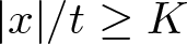 $|x|/t\ge K$.
4.3. Proof of Theorem 2.10
Next, we go back to the general case of (2.1) and prove Theorem 2.10 to obtain (2.30) and (2.31). Let 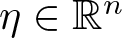 $\eta\in\mathbb{R}^n$ be a constant vector such that
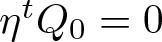 $\eta^tQ_0=0$, where
 $Q_0$ is the eigenprojection of
 $L$ corresponding to the eigenvalue zero. Recall that we only need to prove Theorem 2.10 under Assumption 3.1. Thus, from (3.14)
 $\eta$ takes the form
 \begin{equation}
\eta^t=(0_{1\times n_1}, \eta^t_*),
\end{equation}
where 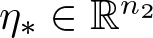 $\eta_*\in\mathbb{R}^{n_2}$.
From (3.38), (3.48) and (4.48) one has 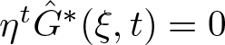 $\eta^t\hat G^*(\xi,t)=0$. Thus, we need to expand
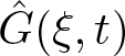 $\hat G(\xi,t)$ for small
 $\xi$ into higher orders to capture the leading term of
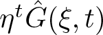 $\eta^t\hat G(\xi,t)$. For this, we recall (3.6) and (3.47),
 \begin{equation}
\hat G(\xi,t)=e^{tE(i\xi)}=\sum_{j=1}^{n'_1}e^{\tilde\lambda_j(i\xi)t}\tilde P_j(i\xi)+\sum_{j=n'_1+1}^{n'}e^{\tilde\lambda_j(i\xi)t}\tilde P_j(i\xi).
\end{equation}
For 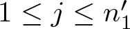 $1\le j\le n'_1$ we consider
 \begin{equation}
\eta^t\tilde P_j(i\xi)=\eta^t[\tilde P_j(0)+i\xi\tilde P'_j(0)+O(1)(i\xi)^2]=i\xi[\eta^t\tilde P_j'(0)]+O(1)\xi^2\equiv i\xi\eta^t_j+O(1)\xi^2.
\end{equation}
Applying (4.49) and (4.50), we have
 \begin{equation}
(i\xi)^l\eta^t\hat G(\xi,t)=\sum_{j=1}^{n'_1}(i\xi)^le^{\tilde\lambda_j(i\xi)t}[i\xi\eta^t_j+O(1)\xi^2]+\sum_{j=n'_1+1}^{n'}(i\xi)^le^{\tilde\lambda_j(i\xi)t}\eta^t\tilde P_j(i\xi).
\end{equation}
Similar to (3.48), the leading term on the right-hand side is
 \begin{equation}
(i\xi)^{l+1}\hat g^*(\xi,t)\equiv(i\xi)^{l+1}\sum_{j=1}^{n'_1}e^{[\tilde\lambda_j'(0)i\xi-\frac12\tilde\lambda^{\prime\prime}_j(0)\xi^2]t}\eta^t_j=(i\xi)^{l+1}\sum_{j=1}^me^{(-\lambda^{(r)}_ji\xi-\mu_j\xi^2)t}\eta^t_j,
\end{equation}
where in the last step we sum up those 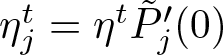 $\eta^t_j=\eta^t\tilde P_j'(0)$,
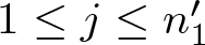 $1\le j\le n'_1$, that share the same pair of
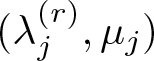 $(\lambda^{(r)}_j, \mu_j)$ and still name those corresponding to distinct pairs
 $\eta^t_j$. The new
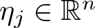 $\eta_j\in \mathbb{R}^n$,
 $1\le j\le m$, are constant vectors, appearing in the first term on the right-hand side of (2.30).
From (4.52), we see that its inverse Fourier transform represents the leading term of 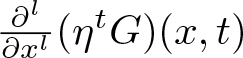 $\frac{\partial^l}{\partial x^l}(\eta^tG)(x,t)$. This is
 \begin{equation}
\frac{\partial^{l+1}}{\partial x^{l+1}}g^*(x,t)=\frac{\partial^{l+1}}{\partial x^{l+1}}\sum_{j=1}^mH(x,t;\lambda^{(r)}_j,\mu_j)\eta^t_j.
\end{equation}
Thus, parallel to (4.1), we set
 \begin{equation}
R^{(l)}_*(x,t)=\frac{\partial^l}{\partial x^l}(\eta^tG)(x,t)-\frac{\partial^{l+1}}{\partial x^{l+1}}g^*(x,t)-\eta^tG^\#_l(x,t),
\end{equation}
and we only need to show that 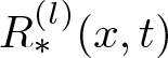 $R^{(l)}_*(x,t)$ is the second term on the right-hand side of (2.30), see (3.71).
For this, we modify (4.2) and write
 \begin{equation}
R^{(l)}_*(x,t)=R^{(l)}_{*1}(x,t)+\eta^tR^{(l)}_2(x,t)+R^{(l)}_{*3}(x,t),
\end{equation}
where  $R^{(l)}_2$ is defined in (4.3), and
 \begin{equation}
\begin{aligned}
R^{(l)}_{*1}(x,t)=&\frac1{2\pi}\int_{-\epsilon}^{\epsilon}e^{ix\xi}[(i\xi)^l\eta^t\hat G(\xi,t)-(i\xi)^{l+1}\hat g^*(\xi,t)]\,d\xi,\\
R^{(l)}_{*3}(x,t)=&\eta^tR^{(l)}_{31}(x,t)+R^{(l)}_{*32}(x,t)+\eta^tR^{(l)}_{33}(x,t),
\end{aligned}
\end{equation}
with 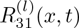 $R^{(l)}_{31}(x,t)$ and
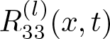 $R^{(l)}_{33}(x,t)$ defined in (4.22), and
 \begin{equation*}
R^{(l)}_{*32}(x,t)=-\frac1{2\pi}\left(\int_{-\infty}^{-\epsilon}+\int_{\epsilon}^{\infty}\right)e^{ix\xi}(i\xi)^{l+1}\hat g^*(\xi,t)\,d\xi.
\end{equation*}
Noting the similarity between 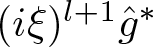 $(i\xi)^{l+1}\hat g^*$ to
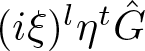 $(i\xi)^l\eta^t\hat G$ and
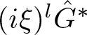 $(i\xi)^l\hat G^*$ to
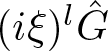 $(i\xi)^l\hat G$, we follow the argument that leads (4.3) to (4.18). First, by substituting (4.51) and (4.52) into (4.56), we have
 \begin{equation}
\begin{aligned}
R^{(l)}_{*1}(x,t)=&\sum_{j=1}^{n'_1}\frac1{2\pi}\int_{-\epsilon}^{\epsilon}e^{ix\xi}(i\xi)^l\{e^{\tilde\lambda_j(i\xi)t}[i\xi\eta^t_j+O(1)\xi^2]-e^{[\tilde\lambda_j'(0)i\xi-\frac12\tilde\lambda^{\prime\prime}_j(0)\xi^2]t}i\xi\eta^t_j\}\,d\xi\\
&+\sum_{j=n'_1+1}^{n'}\frac1{2\pi}\int_{-\epsilon}^{\epsilon}e^{ix\xi}(i\xi)^le^{\tilde\lambda_j(i\xi)t}\eta^t\tilde P_j(i\xi)\,d\xi\\
\equiv&\sum_{j=1}^{n'_1}R^{(l)}_{*1,j}(x,t)+\sum_{j=n'_1+1}^{n'}R^{(l)}_{*1,j}(x,t).
\end{aligned}
\end{equation}
By Taylor expansion we simplify  $R^{(l)}_{*1,j}$ for
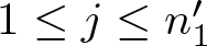 $1\le j\le n'_1$ as
 \begin{equation*}
R^{(l)}_{*1,j}(x,t)= \frac1{2\pi}\int_{-\epsilon}^{\epsilon}e^{ix\xi}(i\xi)^{l+2}e^{(-\lambda^{(r)}_ki\xi-\mu_k\xi^2)t}[O(1)+O(1)\xi^2te^{O(1)\xi^3t}]\,d\xi,
\end{equation*}
where  $1\le k\le m$ is some integer. After moving the path of integration, we note that
 $R^{(l)}_{*1,j}$,
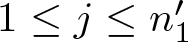 $1\le j\le n'_1$, are parallel to
 $R^{(l)}_{1,j}$ in (4.9), with an extra factor
 $i\xi$ in the integrand. On the other hand, for
 $n'_1+1\le j\le n'$,
 $R^{(l)}_{*1,j}$ are identical to
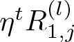 $\eta^tR^{(l)}_{1,j}$, see (4.6). Thus, following the estimation for
 $R^{(l)}_{1}$ that leads to (4.18), we have
 \begin{equation}
|R^{(l)}_{*1}(x,t)|\le C\sum_{k=1}^m(t+1)^{-\frac{l+3}2}e^{-\frac{(x-\lambda_k^{(r)}t)^2}{4\mu_k't}}+Ce^{-t/C}
\end{equation}
for 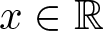 $x\in\mathbb{R}$ and
 $ t \gt 0$.
For the second term on the right-hand side of (4.55), we apply (4.20) to have
 \begin{equation}
|\eta^tR^{(l)}_{2}(x,t)|\le Ct^{-\frac{l+1}2}e^{-t/C}+Ce^{-t/C}.
\end{equation}
For the third term, we follow the estimation of  $R^{(l)}_{32}$ (see (4.25)) to have
 \begin{equation}
|R^{(l)}_{*32}(x,t)|\le Ct^{-\frac{l+2}2}e^{-t/C}.
\end{equation}
Substituting (4.24), (4.25) and (4.60) into (4.56) gives us
 \begin{equation*}
|R^{(l)}_{*3}(x,t)|\le Ce^{-t/C}+Ct^{-\frac{l+2}2}e^{-t/C}.
\end{equation*}
We thus combine (4.55), (4.58)-(4.60) to have, for 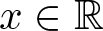 $x\in\mathbb{R}$ and
 $t \gt 0$,
 \begin{equation}
|R^{(l)}_{*}(x,t)|\le C\sum_{k=1}^m(t+1)^{-\frac{l+3}2}e^{-\frac{(x-\lambda_k^{(r)}t)^2}{4\mu_k't}}+Ce^{-t/C}+Ct^{-\frac{l+2}2}e^{-t/C}.
\end{equation}
For 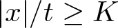 $|x|/t\ge K$ with
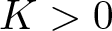 $K \gt 0$ large, we write (4.54) as
 \begin{equation*}
R^{(l)}_*(x,t)=\eta^t\tilde R^{(l)}(x,t)-\frac{\partial^{l+1}}{\partial x^{l+1}}g^*(x,t),
\end{equation*}
where  $\tilde R^{(l)}$ is defined in (4.28). Applying (4.36) and (4.53) gives us
 \begin{equation}
|R^{(l)}_*(x,t)|\le Ce^{-\frac{\nu x^2}{4t}}(e^{-t/C}+t^{-\frac{l+1}2})+C\sum_{j=1}^mt^{-\frac{l+2}2}e^{-\frac{(x-\lambda_j^{(r)}t)^2}{Ct}}
\end{equation}
for 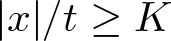 $|x|/t\ge K$.
Following the proof of Theorem 2.3 (starting right after (4.36)), we show that (4.61) and (4.62) imply
 \begin{equation*}
|R^{(l)}_*(x,t)|\le C(t+1)^{-\frac12}t^{-\frac{l+2}2}\sum_{j=1}^me^{-\frac{(x-\lambda_j^{(r)}t)^2}{Ct}},
\end{equation*}
which justifies (2.30). We also prove (2.31) in a similar way.
5. Applications
In this section, we apply our main results to polyatomic gas flows. For both models, (1.4) and (1.9), we construct their Green’s function explicitly by applying Theorem 2.3 and by following Procedure 2.9.
5.1. Thermal non-equilibrium flows
We first consider the models (1.4) for gas flows in both translational and vibrational non-equilibrium, where the translational non-equilibrium is compensated by dissipation mechanisms while the vibrational non-equilibrium is singled out as the sole relaxation process.
Recall that two of the thermodynamic variables are independent in set one (for the translational mode and for all internal modes other than the vibrational mode), and one is independent in set two (for the non-equilibrium vibrational mode). We introduce the following notations,
 \begin{equation}
p=p(v,e_1)=\tilde p(v,T_1),\qquad T_1=T_1(v,e_1),\qquad e_2=\omega(T_2).
\end{equation}
Under those notations we impose the following physical assumptions,
 \begin{equation}
\begin{aligned}
&\tilde p_v=\frac{\partial}{\partial v}\tilde p(v,T_1) \lt 0,\qquad T_{1e_1}=\frac{\partial}{\partial e_1}T_1(v,e_1) \gt 0,\\
&p_{e_1}=\frac{\partial}{\partial e_1}p(v,e_1)\neq0,\qquad\omega'(T) \gt 0.
\end{aligned}
\end{equation}
We note that a state is an equilibrium state if and only if 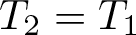 $T_2=T_1$. Let
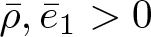 $\bar\rho,\bar e_1 \gt 0$ be constants,
 $\bar T_1=T_1(1/\bar\rho,\bar e_1)$,
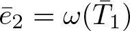 $\bar e_2=\omega(\bar T_1)$ and
 $\bar e=\bar e_1+\bar e_2$. For
 $w=(\rho,\rho u,\rho E,\rho e_2)^t$ in (1.4), we set the corresponding constant equilibrium state as
 \begin{equation}
\bar w=(\bar\rho,0,\bar\rho\bar e,\bar\rho\bar e_2)^t.
\end{equation}
Here, without loss of generality, we have taken  $\bar u=0$.
To linearize (1.4) around  $\bar w$, we note that (1.4) is in the form of (1.1),
 \begin{equation}
w_t+f(w)_x=[B(w)w_x]_x+r(w),
\end{equation}
where
 \begin{equation}
\begin{aligned}
&f(w)=uw+p(0,1,u,0)^t,\qquad r(w)=\Big(0,0,0,\rho[\omega(T_1)-\omega(T_2)]/\tau\Big)^t,\\
&B(w)=\mu vB_1+\kappa vB_2+\nu B_3,\\
&B_1=\begin{pmatrix}0\\1\\u\\0\end{pmatrix}(-u,1,0,0),\qquad B_3=\begin{pmatrix}0\\0\\1\\1\end{pmatrix}(-e_2,0,0,1),\\
&B_2=-\begin{pmatrix}0\\0\\1\\0\end{pmatrix}(vT_{1v}+T_{1e_1}(e_1-\frac{u^2}2),T_{1e_1}u, -T_{1e_1},T_{1e_1}).
\end{aligned}
\end{equation}
The linearization of (1.4) around  $\bar w$ is
 \begin{equation*}
w_t+f'(\bar w)w_x=B(\bar w)w_{xx}+r'(\bar w)(w-\bar w).
\end{equation*}
We reset the perturbation 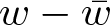 $w-\bar w$ as
 $w$ to arrive at (2.1),
 \begin{equation}
w_t+Aw_x=Bw_{xx}+Lw,
\end{equation}
where
 \begin{equation}
A=f'(\bar w),\qquad B=B(\bar w),\qquad L=r'(\bar w).
\end{equation}
The model for gas flows in both translational and vibrational nonequilibrium is considered in [Reference Zeng31] for space dimensions 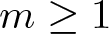 $m\ge1$, which includes (5.4), (5.5) as a special case of
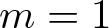 $m=1$. The formulation of
 $f'(w)$ and
 $r'(w)$ is given in Section 4 therein. We cite those results and set
 $w$ to the equilibrium state
 $\bar w$ to have explicit expressions for
 $A,B$ and
 $L$ in (5.7) as follows,
 \begin{equation}
\begin{aligned}
&A=\begin{pmatrix}0&1&0&0\\-v(vp_v+p_{e_1}e_1)&0&vp_{e_1}&-vp_{e_1}\\0&e+vp&0&0\\0&e_2&0&0\end{pmatrix}_{\bar w},\\
&B=\begin{pmatrix}0&0&0&0\\0&\mu v&0&0\\-\kappa v(vT_{1v}+T_{1e_1}e_1)-\nu e_2&0&\kappa vT_{1e_1}&-\kappa vT_{1e_1}+\nu\\-\nu e_2&0&0&\nu\end{pmatrix}_{\bar w},\\
& L
=
-\left.\frac{\omega'(T_1)}{\tau}\right|_{\bar w}
\begin{pmatrix}
0 & 0 & 0 & 0 \\
0 & 0 & 0 & 0 \\
0 & 0 & 0 & 0 \\
vT_{1v}+e_1T_{1e_1}-\dfrac{e_2}{\omega'(T_1)}
& 0
& -T_{1e_1}
& T_{1e_1}+\dfrac{1}{\omega'(T_1)}
\end{pmatrix}_{\bar w}.
\end{aligned}
\end{equation}
A set of structural conditions is proposed in [Reference Zeng31] for a general system of hyperbolic-parabolic balance laws, see Assumption 1.1 therein. Our Assumption 2.1 here is a simplified, linear version of it in the one-dimensional case. It has been verified in [Reference Zeng31] that under the physical assumptions (5.2), the nonlinear system (5.4), (5.5) and its multi-dimensional counterpart satisfy the structural conditions for a variety of choices in dissipation parameters, see Propositions 4.1 and 4.2 therein. Therefore, our linear system (5.6), (5.8) automatically satisfies Assumption 2.1. Precisely, we have the following lemma. Here, for simplicity, we use bar accent to denote a quantity in the equilibrium state  $\bar w$.
Lemma 5.1. Under the assumptions in (5.2), the linear system (5.6), (5.8) satisfies Assumption 2.1 for the following choices of dissipation parameters: (a) 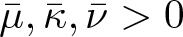 $\bar\mu,\bar\kappa,\bar\nu \gt 0$; (b)
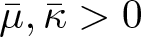 $\bar\mu,\bar\kappa \gt 0$ and
 $\bar\nu=0$; (c)
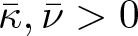 $\bar\kappa,\bar\nu \gt 0$ and
 $\bar\mu=0$; and (d)
 $\bar\kappa \gt $0 and
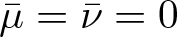 $\bar\mu=\bar\nu=0$.
In Proposition 4.1 of [Reference Zeng31], it is shown that (i) and (ii) of Assumption 2.1 are satisfied under (5.2) and for 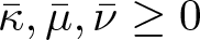 $\bar\kappa,\bar\mu,\bar\nu\ge0$. In particular, the matrix
 $A_0$ in (i) is the Hessian of
 $(-\rho s)$, taken at the constant equilibrium state
 $\bar w$. Here,
 $s$ is the total entropy, see (1.8). In Proposition 4.2 therein, it is further shown that (iii) of Assumption 2.1 is satisfied for the choices of parameters (a)-(d) in Lemma 5.1. Here, we note that
 $\bar\kappa$ is positive in all four cases.
In fact, we can consider  $\bar\kappa=0$ as well. Following a similar argument, one can show that (iii) of Assumption 2.1 is satisfied in case (e)
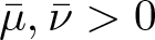 $\bar\mu,\bar\nu \gt 0$ and
 $\bar\kappa=0$, and in case (f)
 $\bar\nu \gt 0$ and
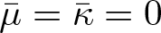 $\bar\mu=\bar\kappa=0$. On the other hand, (iii) of Assumption 2.1 fails when
 $\bar\kappa=\bar\nu=0$ and
 $\bar\mu\ge0$. For conciseness, we omit details of verification.
We now apply Theorem 2.3 to (5.6), (5.8). We use Procedure 2.9 to explicitly construct the Green’s function  $G$.
For this, we use the new variable  $\tilde w$ as defined in (2.9). Noting
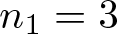 $n_1=3$ and
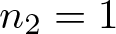 $n_2=1$, we use four components to write
 \begin{equation}
w=\begin{pmatrix}w_1\\w_2\\w_3\\w_4\end{pmatrix}=\begin{pmatrix}\rho-\bar\rho\\\rho u\\ \rho E-\bar\rho\bar e\\ \rho e_2-\bar\rho\bar e_2\end{pmatrix},\qquad\tilde w=\begin{pmatrix}\tilde w_1\\ \tilde w_2\\ \tilde w_3\\ \tilde w_4\end{pmatrix},
\end{equation}
where
 \begin{equation}
\begin{aligned}
\tilde w_1&=w_1,\quad \tilde w_2=w_2,\quad\tilde w_3=w_3,\\
\tilde w_4&=\left.-\frac{\omega'(T_1)}{\tau}\right|_{\bar w}\left\{\left[vT_{1v}+e_1T_{1e_1}-\frac{e_2}{\omega'(T_1)}\right]_{\bar w}w_1-[T_{1e_1}]_{\bar w}w_3\right.\\
&\qquad+\left.\left[T_{1e_1}+\frac1{\omega'(T_1)}\right]_{\bar w}w_4\right\}\equiv k_1w_1+k_3w_3+k_4w_4.
\end{aligned}
\end{equation}
Here, we note that
 \begin{equation}
k_4=-\left.\frac{\omega'(T_1)T_{1e_1}+1}{\tau}\right|_{\bar w} \lt 0.
\end{equation}
Applying (2.10) and (2.12), we have
 \begin{equation}
\begin{aligned}
&\tilde w_w=\begin{pmatrix}1&0&0&0\\0&1&0&0\\0&0&1&0\\k_1&0&k_3&k_4\end{pmatrix},\qquad w_{\tilde w}=\tilde w_w^{-1}=\begin{pmatrix}1&0&0&0\\0&1&0&0\\0&0&1&0\\-k_1/k_4&0&-k_3/k_4&1/k_4\end{pmatrix},\\
&\tilde A=\tilde w_wAw_{\tilde w},\qquad \tilde B=\tilde w_wBw_{\tilde w},\qquad \tilde L=\tilde w_wLw_{\tilde w}={\rm diag}\,(0,0,0,k_4).
\end{aligned}
\end{equation}
Note that 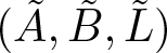 $(\tilde A,\tilde B, \tilde L)$ is the triple that satisfies Assumption 2.1’, which Procedure 2.9 is based upon. Thus, the following formulation is constructed with
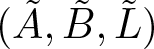 $(\tilde A,\tilde B, \tilde L)$.
In Step 1, we solve the eigen-problem of the third principal minor of  $\tilde A$. First, by direct calculation we have
 \begin{equation}
\tilde A=\begin{pmatrix}0&1&0&0\\a_{21}&0&a_{23}&a_{24}\\0&a_{32}&0&0\\0&a_{42}&0&0\end{pmatrix},
\end{equation}
where
 \begin{equation}
\begin{aligned}
a_{21}=&-\left[v(vp_v+p_{e_1}e_1)-\frac{k_1}{k_4}(vp_{e_1})\right]_{\bar w}\\
=&\left.\frac{-v(vp_v+p_{e_1}e)+\omega'(T_1)v^2(-p_vT_{1e_1}+T_{1v}p_{e_1})}{\omega'(T_1)T_{1e_1}+1}\right|_{\bar w},\\
a_{23}=&\left[vp_{e_1}+\frac{k_3}{k_4}vp_{e_1}\right]_{\bar w}=\left.\frac{vp_{e_1}}{\omega'(T_1)T_{1e_1}+1}\right|_{\bar w},\\
a_{24}=&-\left.\frac{vp_{e_1}}{k_4}\right|_{\bar w}=\left.\frac{vp_{e_1}\tau}{\omega'(T_1)T_{1e_1}+1}\right|_{\bar w},\\
a_{32}=&\left.(e+vp)\right|_{\bar w},\\
a_{42}=&\Big[k_1+k_3(e+vp)+k_4e_2\Big]_{\bar w}=-\left[\frac{\omega'(T_1)}{\tau}(vT_{1v}-T_{1e_1}vp)\right]_{\bar w}\\
=&\left[\frac{\omega'(T_1)vT_1p_{e_1}}{\tau}\right]_{\bar w}.
\end{aligned}
\end{equation}
Here, we have applied the identity
 \begin{equation}
p_{e_1}=(pT_{1e_1}-T_{1v})/T_1
\end{equation}
for  $a_{42}$. Thus, the third principal minor is
 \begin{equation*}
\tilde A^{(r)}=\begin{pmatrix}0&1&0\\a_{21}&0&a_{23}\\0&a_{32}&0\end{pmatrix},
\end{equation*}
which has three distinct eigenvalues
 \begin{equation*}
\lambda_0^{(r)}=0,\qquad\lambda^{(r)}_{\pm}=\pm\sqrt{a_{21}+a_{23}a_{32}}.
\end{equation*}
Using (5.14), we simplify the expression under the square root,
 \begin{equation}
\begin{aligned}
a_{21}+a_{23}a_{32}&=\left[v^2(-p_v+\frac{pp_{e_1}+\omega'(T_1)T_{1v}p_{e_1}}{\omega'(T_1)T_{1e_1}+1})\right]_{\bar w}\\
&=\left[v^2(-p_v+\frac{pp_{e_1}+e^*_{2v}p_{e_1}}{e^*_{2e_1}+1})\right]_{\bar w}\equiv\bar c^2,
\end{aligned}
\end{equation}
where we have used (5.1) to have  $e^*_2=\omega(T_1)=\omega(T_1(v,e_1))$.
It has been shown in [Reference Zeng30] that  $\bar c^2$ defined in (5.16) is a positive number. In fact,
 $\bar c \gt 0$ is the equilibrium speed of sound at
 $\bar w$, see (2.24) and (1.33) in [Reference Zeng30], also see (1.25) in [Reference Zeng26] for the formulation under the Lagrangian coordinates. Thus, the three distinct eigenvalues of
 $\tilde A^{(r)}$ are
 \begin{equation}
\lambda_0^{(r)}=0,\qquad\lambda^{(r)}_{\pm}=\pm\bar c.
\end{equation}
It is straightforward to find normalized left eigenvectors and right eigenvectors as
 \begin{equation}
\begin{aligned}
&l^{(r)}_0=\frac1{\bar c^2}(a_{32},0,-1)\qquad l^{(r)}_{\pm}=\frac1{2\bar c^2}(a_{21},\pm\bar c,a_{23}),\\
&r^{(r)}_0=\begin{pmatrix}a_{23}\\0\\-a_{21}\end{pmatrix},\qquad r^{(r)}_{\pm}=\begin{pmatrix}1\\ \pm\bar c\\a_{32}\end{pmatrix}.
\end{aligned}
\end{equation}
The corresponding projections are
 \begin{equation}
\tilde P_0=\frac1{\bar c^2}\begin{pmatrix}a_{23}a_{32}&0&-a_{23}&0\\0&0&0&0\\-a_{21}a_{32}&0&a_{21}&0\\0&0&0&0\end{pmatrix},\qquad\tilde P_{\pm}=\frac1{2\bar c^2}\begin{pmatrix}a_{21}&\pm\bar c&a_{23}&0\\ \pm a_{21}\bar c&\bar c^2&\pm a_{23}\bar c&0\\a_{21}a_{32}&\pm a_{32}\bar c&a_{23}a_{32}&0\\0&0&0&0\end{pmatrix}.
\end{equation}
We comment that the matrix  $\tilde A^{(r)}$ is the Jacobian matrix of the flux function of the corresponding equilibrium equations. In that case,
 $e_2=e_2^*=\omega(T_1)$, and hence the equation
 $e=e_1+e_2^*(v,e_1)$ implicitly defines
 $e_1$ as a function of
 $e$ and
 $v$, which we write
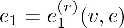 $e_1= e_1^{(r)}(v,e)$. This allows us to regard
 $p$ as a function of
 $v$ and
 $e$ as well,
 \begin{equation*}
p=p(v,e_1^{(r)}(v,e))\equiv p^{(r)}(v,e).
\end{equation*}
Using the notations in (5.1), we can verify that
 \begin{equation*}
a_{21}=\left[-v(vp^{(r)}_v+p^{(r)}_ee)\right]_{\bar w},\qquad a_{23}=\left[vp^{(r)}_e\right]_{\bar w}.
\end{equation*}
Together with  $a_{32}$ in (5.14), these are compared with corresponding entries in
 $A$, see (5.8). Therefore, the eigenvalues
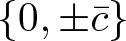 $\{0,\pm\bar c\}$ and the corresponding eigenprojections
 $\{r^{(r)}_0l^{(r)}_0,r^{(r)}_{\pm}l^{(r)}_{\pm}\}$, which give rise to
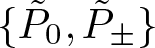 $\{\tilde P_0,\tilde P_{\pm}\}$, are from the spectral decomposition of the Jacobian matrix of the flux function related to the equilibrium flow.
To go back to the original variable  $w$ we set
 \begin{equation}
\begin{aligned}
&P_0=w_{\tilde w}\tilde P_0\tilde w_w=\frac1{\bar c^2}\begin{pmatrix}a_{23}a_{32}&0&-a_{23}&0\\0&0&0&0\\-a_{21}a_{32}&0&a_{21}&0\\-\frac1{k_4}(k_1a_{23}-k_3a_{21})a_{32}&0&\frac1{k_4}(k_1a_{23}-k_3a_{21})&0\end{pmatrix},\\
&P_{\pm}=w_{\tilde w}\tilde P_{\pm}\tilde w_w\\
&\quad =\frac1{2\bar c^2}\begin{pmatrix}a_{21}&\pm\bar c&a_{23}&0\\\pm a_{21}\bar c&\bar c^2&\pm a_{23}\bar c&0\\a_{21}a_{32}&\pm a_{32}\bar c&a_{23}a_{32}&0\\-\frac1{k_4}(k_1\!+\!k_3a_{32})a_{21}&\mp\frac1{k_4}(k_1\!+\!k_3a_{32})\bar c&\!-\frac1{k_4}(k_1\!+\!\!k_3a_{32})a_{23}&0\end{pmatrix}.
\end{aligned}
\end{equation}
Next, we continue into Step 2 of Procedure 2.9 to find diffusion coefficients. From  $\tilde L$ in (5.12), we get
 \begin{equation*}
\tilde S=-\frac1{k_4}\mbox{diag}(0_{3\times3},1).
\end{equation*}
This gives us
 \begin{equation}
\begin{aligned}
\tilde A\tilde S\tilde A&=-\frac1{k_4}[(0,0,0,1)\tilde A^t]^t(0,0,0,1)\tilde A\\
&=-\frac1{k_4}(0,,a_{24},0,0)^t(0,a_{42},0,0)=-\frac1{k_4}a_{24}a_{42}(0,,1,0,0)^t(0,1,0,0)\\
&=\left.\frac{\tau\omega'(T_1)v^2T_1p_{e_1}^2}{[\omega'(T_1)T_{1e_1}+1]^2}\right|_{\bar w}(0,,1,0,0)^t(0,1,0,0),
\end{aligned}
\end{equation}
where we have applied (5.13), (5.14) and (5.10). Using (5.21) and (5.18), we compute the contribution from the relaxation as follows,
 \begin{equation}
\begin{aligned}
&(l_0^{(r)},0)\tilde A \tilde S\tilde A\begin{pmatrix}r_0^{(r)}\\0\end{pmatrix}=0,\\
&(l_{\pm}^{(r)},0)\tilde A \tilde S\tilde A\begin{pmatrix}r_{\pm}^{(r)}\\0\end{pmatrix}=\frac12\left.\frac{\tau\omega'(T_1)v^2T_1p_{e_1}^2}{[\omega'(T_1)T_{1e_1}+1]^2}\right|_{\bar w} \gt 0.
\end{aligned}
\end{equation}
Similarly, the contribution from dissipation mechanisms is
 \begin{equation}
(l_j^{(r)},0)\tilde B\begin{pmatrix}r_j^{(r)}\\0\end{pmatrix}=(l_j^{(r)},0)\tilde w_wBw_{\tilde w}\begin{pmatrix}r_j^{(r)}\\0\end{pmatrix},\qquad j=0, \pm.
\end{equation}
 \begin{equation*}
\begin{aligned}
&(l_0^{(r)},0)\tilde w_w=\frac1{\bar c^2}(a_{32},0,-1,0),\\
&([r_0^{(r)}]^t,0)w_{\tilde w}^t=(a_{23},0,-a_{21},-\frac{k_1}{k_4}a_{23}+\frac{k_3}{k_4}a_{21}).
\end{aligned}
\end{equation*}
Thus,
 \begin{equation}
\begin{aligned}
(l_0^{(r)},0)\tilde B\begin{pmatrix}r_0^{(r)}\\0\end{pmatrix}=&\left\{\frac1{\bar c^2}\kappa v\left[(vT_{1v}+T_{1e_1}e_1)a_{23}+T_{1e_1}(a_{21}-\frac{k_1}{k_4}a_{23}+\frac{k_3}{k_4}a_{21})\right]\right.\\
&+\left.\frac{\nu}{\bar c^2}(e_2a_{23}+\frac{k_1}{k_4}a_{23}-\frac{k_3}{k_4}a_{21})\right\}_{\bar w}\equiv \frac1{\bar c^2}kv\mu_{01}+\frac{\nu}{\bar c^2}\mu_{02}.
\end{aligned}
\end{equation}
Next, we apply (5.10) and (5.14) to have
 \begin{equation*}
\begin{aligned}
-\frac{k_1}{k_4}a_{23}+\frac{k_3}{k_4}a_{21}
=&-\frac1{[\omega'(T_1)T_{1e_1}+1]^2_{\bar w}}\left\{-vp_{e_1}e_2+\omega'(T_1)vp_{e_1}(T_{1v}v+T_{1e_1}e_1)\right.\\
&\left.-\omega'(T_1)T_{1e_1}v(vp_v+ep_{e_1})\!+\![\omega'(T_1)]^2T_{1e_1}v^2(p_{e_1}T_{1v}-p_vT_{1e_1})\right\}_{\bar w}\\
=&-\frac1{[\omega'(T_1)T_{1e_1}+1]^2_{\bar w}}\left\{-vp_{e_1}e_2[1+\omega'(T_1)T_{1e_1}]\right.\\
&\left.+\omega'(T_1)v^2(p_{e_1}T_{1v}-p_vT_{1e_1})[1+\omega'(T_1)T_{1e_1}]\right\}_{\bar w}\\
=&\frac1{[\omega'(T_1)T_{1e_1}+1]_{\bar w}}\left[vp_{e_1}e_2-\omega'(T_1)v^2(p_{e_1}T_{1v}-p_vT_{1e_1})\right]_{\bar w}.
\end{aligned}
\end{equation*}
This gives us
 \begin{equation*}
a_{21}-\frac{k_1}{k_4}a_{23}+\frac{k_3}{k_4}a_{21}=\left.\frac{-v(vp_v+p_{e_1}e_1)}{\omega'(T_1)T_{1e_1}+1}\right|_{\bar w}.
\end{equation*}
Applying the identity
 \begin{equation}
\tilde p_v=p_v-T_{1v}p_{e_1}/T_{1e_1},
\end{equation}
we have
 \begin{equation}
\begin{aligned}
\mu_{01}&=\left[(vT_{1v}+T_{1e_1}e_1)a_{23}+T_{1e_1}(a_{21}-\frac{k_1}{k_4}a_{23}+\frac{k_3}{k_4}a_{21})\right]_{\bar w}\\
&=\left\{\frac v{\omega'(T_1)T_{1e_1}+1}[p_{e_1}(vT_{1v}+T_{1e_1}e_1)-T_{1e_1}(vp_v+p_{e_1}e_1)]\right\}_{\bar w}\\
&=\left[\frac v{\omega'(T_1)T_{1e_1}+1}(p_{e_1}vT_{1v}-T_{1e_1}vp_v)\right]_{\bar w}=\left.\frac{v^2T_{1e_1}(-\tilde p_v)}{\omega'(T_1)T_{1e_1}+1}\right|_{\bar w} \gt 0.
\end{aligned}
\end{equation}
Similarly,
 \begin{equation}
\mu_{02}=\bar e_2a_{23}+\frac{k_1}{k_4}a_{23}-\frac{k_3}{k_4}a_{21}=\left.\frac{\omega'(T_1)v^2T_{1e_1}(-\tilde p_v)}{\omega'(T_1)T_{1e_1}+1}\right|_{\bar w} \gt 0.
\end{equation}
Substituting (5.26) and (5.27) into (5.24), we arrive at
 \begin{equation}
(l^{(r)}_0,0)\tilde B\begin{pmatrix}r_0^{(r)}\\0\end{pmatrix}=\left.\frac{v^2T_{1e_1}(-\tilde p_v)[\kappa v+\nu \omega'(T_1)]}{\bar c^2[\omega'(T_1)T_{1e_1}+1]}\right|_{\bar w}\ge0
\end{equation}
for 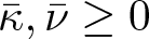 $\bar\kappa,\bar\nu\ge0$.
Finally, combining (5.22) and (5.28), we obtain  $\mu_0$ as defined in (2.25),
 \begin{equation}
\mu_0=\left.\frac{v^2T_{1e_1}(-\tilde p_v)[\kappa v+\nu \omega'(T_1)]}{\bar c^2[\omega'(T_1)T_{1e_1}+1]}\right|_{\bar w} \gt 0
\end{equation}
for cases (a)-(f). (On the other hand, 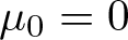 $\mu_0=0$ if
 $\bar\kappa=\bar\nu=0$ while
 $\bar\mu\ge0$.)
With similar calculation we find
 \begin{equation}
(l^{(r)}_{\pm},0)\tilde B\begin{pmatrix}r_{\pm}^{(r)}\\0\end{pmatrix}=\left\{\frac{v^2p_{e_1}^2T_1[\kappa v+\nu \omega'(T_1)]}{2\bar c^2[\omega'(T_1)T_{1e_1}+1]^2}+\frac{\mu v}2\right\}_{\bar w}\ge0
\end{equation}
for 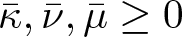 $\bar\kappa,\bar\nu,\bar\mu\ge0$. Therefore, applying (5.22) and (5.30) to (2.25) gives us
 \begin{equation}
\mu_{\pm}=\left.\frac{v^2p^2_{e_1}T_1}{2[\omega'(T_1)T_{1e_1}+1]^2}\{\tau\omega'(T_1)+
[\kappa v+\nu \omega'(T_1)]/\bar c^2\}+\frac{\mu}2v\right|_{\bar w} \gt 0
\end{equation}
for 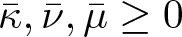 $\bar\kappa,\bar\nu,\bar\mu\ge0$.
We comment that  $\mu_{\pm}$ are always positive while
 $\mu_0$ can be zero if
 $\bar\kappa=\bar\nu=0$. In that case, the Kawashima–Shizuta condition fails. Intuitively, we expect that the corresponding heat kernel degenerates to a non-decaying
 $\delta$-function along the particle path. Indeed, it is verified for the inviscid case
 $\bar\kappa=\bar\nu=\bar \mu=0$ in [Reference Zeng26].
We now move on to Step 3 in Procedure 2.9. While the heat kernels in (2.5) are formulated uniformly above for cases (a)-(f), the singular part needs to be constructed case by case. Here, we consider the physically relevant one, 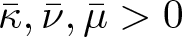 $\bar\kappa,\bar\nu,\bar \mu \gt 0$. In this case,
 $\tilde B$ has four eigenvalues,
 \begin{equation}
\sigma'_0=0,\quad\sigma'_1=\mu v\Big|_{\bar w}\quad\sigma'_2=\kappa vT_{1e_1}\Big|_{\bar w}\quad\sigma'_3=\nu \Big|_{\bar w},
\end{equation}
see (5.12) and (5.8). The eigenprojection corresponding to zero is
 \begin{equation}
\begin{aligned}
\tilde Q'_0&=\tilde w_w(1,0,e+vT_{1v}/T_{1e_1},e_2)^t\Big|_{\bar w}(1,0,0,0)w_{\tilde w}\\
&=(1,0,e+vT_{1v}/T_{1e_1},0)^t\Big|_{\bar w}(1,0,0,0)\equiv\eta_1(1,0,0,0).
\end{aligned}
\end{equation}
This implies
 \begin{equation}
\tilde Q'_0\tilde A\tilde Q'_0=(1,0,e+vT_{1v}/T_{1e_1},0)^t_{\bar w}(0,1,0,0)(1,0,e+vT_{1v}/T_{1e_1},0)^t_{\bar w}(1,0,0,0)=0.
\end{equation}
The right-hand side of (5.34) is the spectral decomposition of  $\tilde Q'_0\tilde A\tilde Q'_0$ in the range of
 $\tilde Q'_0$, i.e.,
 $\alpha=0$,
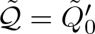 $\tilde{\mathcal{Q}}=\tilde Q'_0$.
We continue into Step 4 of Procedure 2.9. For  $\tilde B$ we find eigenprojections corresponding to
 $\sigma'_k$,
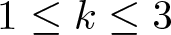 $1\le k\le3$, as
 \begin{equation}
\begin{aligned}
&\tilde Q'_1=\tilde w_w(0,1,0,0)^t(0,1,0,0)w_{\tilde w},\\
&\tilde Q'_2=\tilde w_w(0,0,1,0)^t(-vT_{1v}/T_{1e_1}-e_1,0,1,-1)\Big|_{\bar w}w_{\tilde w},\\
&\tilde Q'_3=\tilde w_w(0,0,1,1)^t(-\bar e_2,0,0,1)w_{\tilde w}.
\end{aligned}
\end{equation}
By (2.28),
 \begin{equation}
\tilde S'=\left[\frac1{\mu v}\tilde Q'_1+\frac1{\kappa vT_{1e_1}}\tilde Q'_2+\frac1{\nu}\tilde Q'_3\right]_{\bar w}.
\end{equation}
Thus, applying (5.33), (5.12)-(5.14), (5.36), and (5.25), we have
 \begin{equation}
\begin{aligned}
&\tilde{\mathcal{Q}}\tilde A\tilde S'\tilde A \tilde{\mathcal{Q}}=\tilde Q'_0\tilde A\tilde S'\tilde A \tilde Q'_0
=\eta_1(0,1,0,0)\tilde S'(0,-v^2(p_v-p_{e_1}T_{1v}/T_{1e_1}),0,0)^t(1,0,0,0)\\
&=\eta_1\left[\frac1{\mu v}v^2(-p_v+p_{e_1}T_{1v}/T_{1e_1})\right]_{\bar w}(1,0,0,0)=\left[-\frac v{\mu}\tilde p_v\right]_{\bar w}\tilde Q'_0.
\end{aligned}
\end{equation}
Similarly, from (5.12), we have
 \begin{equation}
\tilde{\mathcal{Q}}\tilde L\tilde{\mathcal{Q}}=\tilde Q'_0\,\mbox{diag}(0,0,0,k_4)\,\tilde Q'_0=0.
\end{equation}
Combining (5.37) and (5.38) gives us
 \begin{equation}
\tilde{\mathcal{Q}}(\tilde A\tilde S'\tilde A-\tilde L) \tilde{\mathcal{Q}}=\left[-\frac v{\mu}\tilde p_v\right]_{\bar w}\tilde Q'_0,
\end{equation}
where the right-hand side is the spectral decomposition of the matrix on the left-hand side in the range of 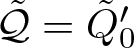 $\tilde{\mathcal{Q}}=\tilde Q'_0$. Therefore,
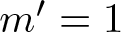 $m'=1$,
 \begin{equation}
\beta=\left[-\frac v{\mu}\tilde p_v\right]_{\bar w} \gt 0,
\end{equation}
and 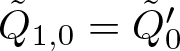 $\tilde Q_{1,0}=\tilde Q'_0$. To go back to the original variable
 $w$ we set
 \begin{equation}
Q_{1,0}=w_{\tilde w}\tilde Q'_0\tilde w_w=\begin{pmatrix}1&0&0&0\\0&0&0&0\\e+\frac{vT_{1v}}{T_{1e_1}}&0&0&0\\e_2&0&0&0\end{pmatrix}_{\bar w}.
\end{equation}
Using the information obtained in all four steps, we write the Green’s function of the Cauchy problem of (5.6), (5.8), given by Theorem 2.3, as
 \begin{equation}
\begin{aligned}
G(x,t)=&H(x,t;-\bar c,\mu_-)P_-+H(x,t;0,\mu_0)P_0+H(x,t;\bar c,\mu_+)P_+\\
&+O(1)(t+1)^{-\frac12}[H(x,t;-\bar c,C)+H(x,t;0,C)+H(x,t;\bar c,C)]\\
&+e^{[\frac v{\mu}\tilde p_v]_{\bar w}t}\delta(x)Q_{1,0},
\end{aligned}
\end{equation}
where  $\bar c,\mu_0,\mu_{\pm}, P_0,P_{\pm}$ and
 $Q_{1,0}$ are given in (5.16), (5.29), (5.31), (5.20) and (5.41), and
 $C \gt 0$ is some constant,
We comment that the heat kernels in (5.42) are common to all choices (a)–(f) of dissipation parameters, where  $\mu_0$ and
 $\mu_{\pm}$ have explicit dependence on those parameters in (5.29) and (5.31). On the other hand, the
 $\delta$-function in (5.42) is for the physically relevant case (a). From the point of view of PDE theory, we list corresponding results for other cases to illustrate how the matrix
 $B$ impacts the singular part in
 $G$. Since the construction for other cases is parallel to that of case (a), we omit details of the calculation.
We write  $G$ for all cases as
 \begin{equation}
\begin{aligned}
G(x,t)=&H(x,t;-\bar c,\mu_-)P_-+H(x,t;0,\mu_0)P_0+H(x,t;\bar c,\mu_+)P_+\\
&+O(1)(t+1)^{-\frac12}[H(x,t;-\bar c,C)+H(x,t;0,C)+H(x,t;\bar c,C)]+D.
\end{aligned}
\end{equation}
Then  $D$ is given below.
(b) For 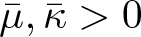 $\bar \mu,\bar\kappa \gt 0$ and
 $\bar\nu=0$,
 \begin{equation*}
D=e^{[\frac v{\mu}\tilde p_v]_{\bar w}t}\delta(x)Q_{1,0}+e^{-t/\bar\tau}\delta(x)Q_{2,0},
\end{equation*}
where  $Q_{1,0}$ is given in (5.41), and
 \begin{equation}
Q_{2,0}=(0,0,1,1)^t(-\bar e_2, 0,0,1).
\end{equation}
(c) For 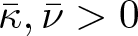 $\bar\kappa,\bar\nu \gt 0$ and
 $\bar\mu=0$,
 \begin{equation*}
D=e^{-\beta t}\delta(x+\alpha t)Q_{-,0}+e^{-\beta t}\delta(x-\alpha t)Q_{+,0},
\end{equation*}
where
 \begin{equation}
\begin{aligned}
&\alpha=\Big[v\sqrt{-\tilde p_v}\Big]_{\bar w} \gt 0,\qquad\beta=\left[\frac{vp_{e_1}^2T_1}{2\kappa T_{1e_1}^2}\right]_{\bar w} \gt 0,\\
&Q_{\pm,0}=\pm\frac1{2\alpha}(1,\pm\alpha,e+vT_{1v}/T_{1e_1},e_2)^t_{\bar w}(\pm\alpha,1,0,0).
\end{aligned}
\end{equation}
(d) For  $\bar\kappa \gt 0$ and
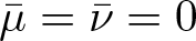 $\bar\mu=\bar\nu=0$,
 \begin{equation*}
D=e^{-\beta t}\delta(x+\alpha t)Q_{-,0}+e^{-t/\bar\tau}\delta(x)Q_{2,0}+e^{-\beta t}\delta(x-\alpha t)Q_{+,0},
\end{equation*}
where  $\alpha,\beta$ and
 $Q_{\pm,0}$ are those defined in (5.45), and
 $Q_{2,0}$ is defined in (5.44).
(e) We note that
 \begin{equation}
\begin{aligned}
c_f^2&\equiv(pp_{e_1}-p_v)v^2=-v^2\frac{\partial}{\partial v}p(v,e_1(v,s_1))=-v^2\frac{\partial}{\partial v}\tilde p(v,T_1(v,s_1))\\
&=-v^2\tilde p_v+v^2T_1\Big[\frac{\partial}{\partial T_1}\tilde p(v,T_1)\Big]^2T_{1e_1} \gt 0.
\end{aligned}
\end{equation}
In fact, 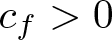 $c_f \gt 0$ is the frozen speed of sound. We set
 \begin{equation*}
\bar c_f=c_f\Big|_{\bar w}.
\end{equation*}
Then for 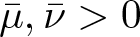 $\bar\mu,\bar\nu \gt 0$, and
 $\bar\kappa=0$,
 \begin{equation*}
D=e^{-\beta_- t}\delta(x)Q_{-,0}+e^{-\beta_+ t}\delta(x)Q_{+,0},
\end{equation*}
where
 \begin{equation}
\begin{aligned}
\beta_{\pm}&=\frac12(c_1\pm\sqrt c_2),\\
c_1&=\left[\frac{-vp_v+p_{e_1}vp}{\mu}+\frac{\omega'(T_1)T_{1e_1}}{\tau}\right]_{\bar w}=\left[\frac{c_f^2}{\mu v}+\frac{\omega'(T_1)T_{1e_1}}{\tau}\right]_{\bar w} \gt 0,\\
c_2&=c_1^2-4\left.\frac{\omega'(T_1)(-vp_vT_{1e_1}+p_{e_1}T_{1v}v)}{\mu\tau}\right|_{\bar w}\\
&=\left[\frac{-vp_v+p_{e_1}vp}{\mu}-\frac{\omega'(T_1)T_{1e_1}}{\tau}\right]^2_{\bar w}+4\left.\frac{\omega'(T_1)p_{e_1}^2vT_1}{\mu\tau}\right|_{\bar w} \gt 0,\\
Q_{\pm,0}&=\pm\frac1{\beta_+-\beta_-}\begin{pmatrix}1\\0\\e+\frac{vp_v+\mu\beta_{\pm}}{p_{e_1}}\\e_2\end{pmatrix}_{\bar w}\Big(\frac{-vp_v-p_{e_1}e_1}{\mu}-\beta_{\mp},0,\frac{p_{e_1}}{\mu},-\frac{p_{e_1}}{\mu}\Big)_{\bar w}.
\end{aligned}
\end{equation}
Here, we have used (5.15) for  $c_2$. We can also use (5.25) to write
 \begin{equation*}
c_2=c_1^2+4\frac{\omega'(T_1)T_{1e_1}v\tilde p_v}{\mu\tau} \lt c_1^2.
\end{equation*}
Thus,  $\beta_+ \gt \beta_- \gt 0$.
(f) For  $\bar\nu \gt 0$ and
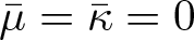 $\bar\mu=\bar\kappa=0$,
 \begin{equation*}
D=e^{-\beta t}\delta(x+\bar c_f t)Q_{-,0}+e^{-\beta_0t}\delta(x)Q_{0,0}+e^{-\beta t}\delta(x-\bar c_f t)Q_{+,0},
\end{equation*}
where
 \begin{equation*}
\begin{aligned}
&\beta=\left.\frac{v^2p_{e_1}^2T_1\omega'(T_1)}{2\tau c_f^2}\right|_{\bar w} \gt 0,\qquad\beta_0=\left.\frac{v^2T_{1e_1}(-\tilde p_v)\omega'(T_1)}{\tau c_f^2}\right|_{\bar w} \gt 0,\\
&Q_{\pm,0}=\frac1{2\bar c_f^2}\begin{pmatrix}1\\ \pm c_f\\e+vp\\e_2\end{pmatrix}_{\bar w}\Big(-v(vp_v+p_{e_1}e_1),\pm c_f,vp_{e_1},-vp_{e_1}\Big)_{\bar w},\\
&Q_{0,0}=\frac1{\bar c_f^2}\begin{pmatrix}vp_{e_1}\\0\\v(vp_v+p_{e_1}e)\\vp_{e_1}e_2\end{pmatrix}_{\bar w}
\Big(e_1+vp,0,-1,1\Big)_{\bar w}.
\end{aligned}
\end{equation*}
5.2. Two-temperature Navier–Stokes type model
Next, we consider the model (1.9), which is also in the form of (1.1),
 \begin{equation}
w_t+f(w)_x=[B(w)w_x]_x+r(w),
\end{equation}
where  $w=(\rho,\rho u,\rho E,\rho T_2)^t$ with
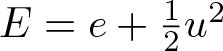 $E=e+\frac12 u^2$,
 \begin{equation}
\begin{aligned}
&f(w)=uw+p(0,1,u,0)^t,\qquad r(w)=\Big(0,0,0,\frac3{3+D}\theta A_c(T)\rho^2(T_1-T_2)\Big)^t,\\
&B(w)=\frac1{\rho}\big(\mu_{\rm tr} B_1+\lambda_{\rm tr}B_{21}+\frac2{DR}\lambda_{\rm int} B_{22}\big),\\
&B_1=\begin{pmatrix}0\\1\\u\\0\end{pmatrix}(-u,1,0,0),\qquad B_{22}=\begin{pmatrix}0\\0\\0\\1\end{pmatrix}(-T_2,0,0,1),\\
&B_{21}=\begin{pmatrix}0\\0\\1\\0\end{pmatrix}\Big(\frac{u^2}{3R}-T_1-\frac D5T_2,-\frac{2u}{3R},\frac2{3R},-\frac{2D}{15}\Big).
\end{aligned}
\end{equation}
Here, we have applied (1.10) and (1.12). Noting  $\lambda_{\rm int}$ and
 $\lambda_{\rm tr}$ are not independent, see (1.11), we further have
 \begin{equation}
B(w)=\frac1{\rho}\big(\mu_{\rm tr} B_1+\lambda_{\rm tr}B_{2}\big),
\end{equation}
where
 \begin{equation}
\begin{aligned}
B_2&=B_{21}+\frac2{5R}B_{22}\\
&=\begin{pmatrix}0\\0\\1\\0\end{pmatrix}\Big(\frac{u^2}{3R}-T_1-\frac D5T_2,-\frac{2u}{3R},\frac2{3R},-\frac{2D}{15}\Big)
+\begin{pmatrix}0\\0\\0\\1\end{pmatrix}(-\frac2{5R}T_2,0,0,\frac2{5R}).
\end{aligned}
\end{equation}
We recalled that a state is an equilibrium state if and only if  $T=T_1=T_2$. Thus, letting
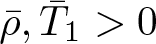 $\bar\rho,\bar T_1 \gt 0$ be constants, we take a constant equilibrium state as
 \begin{equation}
\bar w=(\bar\rho,0,\bar\rho\bar e,\bar\rho\bar T_1)^t,\qquad\bar e=\frac{3+D}2R\bar T_1.
\end{equation}
We linearize (5.48) around  $\bar w$ and reset
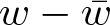 $w-\bar w$ as
 $w$ to have
 \begin{equation}
w_t+Aw_x=Bw_{xx}+Lw,
\end{equation}
where
 \begin{equation*}
A=f'(\bar w),\qquad B=B(\bar w), \qquad L=r'(\bar w).
\end{equation*}
From (5.49)-(5.51) and by direct calculation, we further have
 \begin{equation}
\begin{aligned}
A&=\begin{pmatrix}0&1&0&0\\0&0&\frac23&-\frac D3R\\0&\frac{5+D}2R\bar T_1&0&0\\0&\bar T_1&0&0\end{pmatrix},\\
B&=\begin{pmatrix}0&0&0&0\\0&\frac{\bar\mu_{\rm tr}} {\bar \rho}&0&0\\-\bar\lambda_{\rm tr}\frac{5+D}5\frac{\bar T_1}{\bar\rho}&0&\bar\lambda_{\rm tr}\frac2{3R\bar\rho}&-\bar\lambda_{\rm tr}\frac{2D}{15\bar\rho}\\-\bar\lambda_{\rm tr}\frac2{5R}\frac{\bar T_1}{\bar\rho}&0&0&\bar\lambda_{\rm tr}\frac2{5R\bar\rho}\end{pmatrix},\\
L&=-\frac3{3+D}\theta A_c(\bar T_1)\bar\rho\begin{pmatrix}0\\0\\0\\1\end{pmatrix}\Big(0,0,-\frac2{3R},\frac{3+D}3\Big),
\end{aligned}
\end{equation}
where  $\bar\mu_{\rm tr}=\mu_{\rm tr}(\bar T_1,\bar T_1)$ and
 $\bar\lambda_{\rm tr}=\lambda_{\rm tr}(\bar T_1,\bar T_1)$.
Lemma 5.2. The linearized two-temperature Navier–Stokes type model (5.53), with  $A,B$ and
 $L$ defined in (5.54), satisfies Assumption 2.1.
Proof. To verify condition (i) in Assumption 2.1, we take a symmetrizer
 \begin{equation*}
A_0=\begin{pmatrix}\frac{5+D}2R\bar T_1^2&0&-\bar T_1&0\\0&\bar T_1&0&0\\-\bar T_1&0&\frac2{3R}&-\frac D3\\0&0&-\frac D3&\frac{(3+D)D}6R\end{pmatrix},
\end{equation*}
which is symmetric, positive definite, with
 \begin{equation*}
\begin{aligned}
A_0A&=\begin{pmatrix}0&0&0&0\\0&0&\frac23\bar T_1&-\frac D3R\bar T_1\\0&\frac23\bar T_1&0&0&\\0&-\frac D3R\bar T_1&0&0\end{pmatrix},\\
A_0B&=\begin{pmatrix}\bar\lambda_{\rm tr}\frac{5+D}5\frac{\bar T_1^2}{\bar\rho}&0&-\bar\lambda_{\rm tr}\frac2{3R}\frac{\bar T_1}{\bar\rho}&\bar\lambda_{\rm tr}\frac{2D}{15}\frac{\bar T_1}{\bar\rho}\\0&\bar\mu_{\rm tr}\frac{\bar T_1}{\bar\rho}&0&0\\-\bar\lambda_{\rm tr}\frac2{3R}\frac{\bar T_1}{\bar\rho}&0&\bar\lambda_{\rm tr}\frac4{9R^2\bar\rho}&-\bar\lambda_{\rm tr}\frac{2D}{9R\bar\rho}\\ \bar\lambda_{\rm tr}\frac{2D}{15}\frac{\bar T_1}{\bar\rho}&0&-\bar\lambda_{\rm tr}\frac{2D}{9R\bar\rho}& \bar\lambda_{\rm tr}(\frac D9+\frac15)\frac D{\bar\rho}\end{pmatrix},\\
A_0L&=-\frac{3D}{2(3+D)}\theta A_c(\bar T_1)R\bar\rho\begin{pmatrix}0\\0\\-\frac2{3R}\\ \frac{3+D}3\end{pmatrix}\Big(0,0,-\frac2{3R},\frac{3+D}3\Big).
\end{aligned}
\end{equation*}
It is clear that  $A_0A$ and
 $A_0B$ are symmetric, and
 $A_0L$ is symmetric, negative semi-definite. Note that
 $A_0^{1/2}BA_0^{-1/2}=A_0^{-1/2}A_0BA_0^{-1/2}$ is symmetric and similar to
 $B$. From (5.54), all eigenvalues of
 $B$ are nonnegative. This implies that
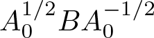 $A_0^{1/2}BA_0^{-1/2}$, and hence
 $A_0B$, is symmetric, positive semi-definite.
For condition (ii), from (5.54) it is clear that (5.53) has 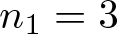 $n_1=3$ conservation laws, with
 $L_{22}=-\theta A_c(\bar T_1)\bar\rho \lt 0$.
To verify condition (iii), we note that the null space  $\mathbb N_1$ of
 $B$ is one-dimensional and the null space
 $\mathbb N_2$ of
 $L$ is three-dimensional, as zero is a simple eigenvalue of
 $B$ and a triple eigenvalue of
 $L$. By direct calculation one can find
 \begin{equation*}
\mathbb N_1={\rm span}\left\{\begin{pmatrix}1\\0\\ \frac{3+D}2R\bar T_1\\ \bar T_1\end{pmatrix}\right\},\qquad\mathbb N_2={\rm span}\left\{\begin{pmatrix}1\\0\\0\\0\end{pmatrix},\begin{pmatrix}0\\1\\0\\0\end{pmatrix},\begin{pmatrix}0\\0\\ \frac{3+D}2R\\1\end{pmatrix}\right\}.
\end{equation*}
Thus, 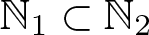 $\mathbb N_1\subset\mathbb N_2$ and hence
 $\mathbb N_1\cap\mathbb N_2=\mathbb N_1$. Again, by direct calculation one can verify that
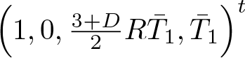 $\Big(1,0, \frac{3+D}2R\bar T_1,\bar T_1\Big)^t$ is not an eigenvector of
 $A$. That is,
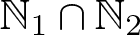 $\mathbb N_1\cap\mathbb N_2$ contains no eigenvectors of
 $A$.
Remark 5.3. In a recent paper [Reference Zeng36], it is shown that the two-temperature Navier–Stokes type model (1.9) and its multi-dimensional full system satisfy a set of structural conditions. The set is an extended, nonlinear version of Assumption 2.1. This allows the  $L^2$ theory for a general nonlinear system built in [Reference Zeng31]-[Reference Zeng34] to apply to small, classical solutions of (1.9) and its full system.
Next, we define the new variable  $\tilde w$ as in (2.9). Noting
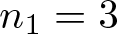 $n_1=3$ we write
 \begin{equation}
w=\begin{pmatrix}w_1\\w_2\\w_3\\w_4\end{pmatrix}=\begin{pmatrix}\rho-\bar\rho\\ \rho u\\ \rho E-\bar\rho\bar e\\ \rho T_2-\bar\rho \bar T_1\end{pmatrix},\qquad\tilde w=\begin{pmatrix}\tilde w_1\\ \tilde w_2\\ \tilde w_3\\ \tilde w_4\end{pmatrix},
\end{equation}
where
 \begin{equation}
\begin{aligned}
&\tilde w_1=w_1,\quad\tilde w_2=w_2,\quad\tilde w_3=w_3,\\
&\tilde w_4=-\frac{3}{3+D}\theta A_c(\bar T_1)\bar\rho\Big(-\frac2{3R}w_3+\frac{3+D}3w_4\Big)\equiv k_3w_3+k_4w_4.
\end{aligned}
\end{equation}
Then
 \begin{equation}
\tilde w_w=\begin{pmatrix}1&0&0&0\\0&1&0&0\\0&0&1&0\\0&0&k_3&k_4\end{pmatrix},\qquad w_{\tilde w}=\tilde w_w^{-1}=\begin{pmatrix}1&0&0&0\\0&1&0&0\\0&0&1&0\\0&0&-\frac{k_3}{k_4}&\frac1{k_4}\end{pmatrix}.
\end{equation}
Correspondingly, we define
 \begin{equation}
\tilde A=\tilde w_wAw_{\tilde w},\quad\tilde B=\tilde w_wBw_{\tilde w},\quad\tilde L=\tilde w_wLw_{\tilde w}={\rm diag}(0,0,0,k_4),
\end{equation}
which form the triple that satisfies Assumption 2.1’.
Now we follow Procedure 2.9 to construct the Green’s function for (5.53), (5.54). From (5.54) and (5.56)-(5.58) and by direct calculation,
 \begin{equation}
\begin{aligned}
&\tilde A=\begin{pmatrix}0&1&0&0\\0&0&a_{23}&a_{24}\\0&a_{32}&0&0\\0&a_{42}&0&0\end{pmatrix},\\
&a_{23}=\frac23+\frac D3R\frac{k_3}{k_4}=\frac2{3+D},\qquad a_{24}=-\frac D3R\frac1{k_4}=\frac{DR}{3\bar\rho}[\theta A_c(\bar T_1)]^{-1},\\
&a_{32}=\frac{5+D}2R\bar T_1,\qquad a_{42}=k_3\frac{5+D}2R\bar T_1+k_4\bar T_1=\frac2{3+D}\theta A_c(\bar T_1)\bar\rho\bar T_1.
\end{aligned}
\end{equation}
Thus, the third principal minor of  $\tilde A$ is
 \begin{equation*}
\tilde A^{(r)}=\begin{pmatrix}0&1&0\\0&0&\frac2{3+D}\\0&\frac{5+D}2R\bar T_1&0\end{pmatrix},
\end{equation*}
which has three distinct eigenvalues,
 \begin{equation}
\lambda_0^{(r)}=0,\qquad\lambda_{\pm}^{(r)}=\pm\bar c,\quad \bar c=\sqrt{\frac{5+D}{3+D}RT_1}.
\end{equation}
The normalized left eigenvectors and right eigenvectors are
 \begin{equation}
\begin{aligned}
&l_0^{(r)}=\frac1{\bar c^2}\Big(\frac{5+D}2R\bar T_1,0,-1\Big),\qquad l_{\pm}^{(r)}=\frac1{2\bar c^2}\Big(0,\pm\bar c,\frac2{3+D}\Big),\\
&r_0^{(r)}=\begin{pmatrix}\frac2{3+D}\\0\\0\end{pmatrix},\qquad r_{\pm}^{(r)}=\begin{pmatrix}1\\ \pm\bar c\\ \frac{5+D}2R\bar T_1\end{pmatrix}.
\end{aligned}
\end{equation}
The corresponding projections are
 \begin{equation}
\tilde P_0=\frac1{\bar c^2}\begin{pmatrix}\bar c^2&0&-\frac2{3+D}&0\\0&0&0&0\\0&0&0&0\\0&0&0&0\end{pmatrix},\qquad\tilde P_{\pm}=\frac1{2\bar c^2}\begin{pmatrix}0&\pm\bar c&\frac2{3+D}&0\\0&\bar c^2&\pm\frac2{3+D}\bar c&0\\0&\pm\frac{5+D}2R\bar T_1\bar c&\bar c^2&0\\0&0&0&0\end{pmatrix}.
\end{equation}
To go back to the original variable  $w$ we set
 \begin{equation}
P_0=w_{\tilde w}\tilde P_0\tilde w_w=\tilde P_0,\qquad P_{\pm}=w_{\tilde w}\tilde P_{\pm}\tilde w_w=\frac1{2\bar c^2}\begin{pmatrix}0&\pm\bar c&\frac2{3+D}&0\\0&\bar c^2&\pm\frac2{3+D}\bar c&0\\0&\pm\frac{5+D}2R\bar T_1\bar c&\bar c^2&0\\0&\pm\frac{\bar c^3}R&\frac{2\bar c^2}{(3+D)R}&0\end{pmatrix}.
\end{equation}
Next, we find diffusion coefficients. From (5.58), we have
 \begin{equation*}
\tilde S=-\frac1{k_4}{\rm diag}(0_{3\times3},1).
\end{equation*}
With (5.59) and (5.56), we further have
 \begin{equation*}
\tilde A\tilde S\tilde A=-\frac1{k_4}a_{42}a_{24}(0,1,0,0)^t(0,1,0,0)=\frac{2D}{3(3+D)}\frac{R\bar T_1}{\theta A_c(\bar T_1)\bar\rho}(0,1,0,0)^t(0,1,0,0).
\end{equation*}
Applying (5.61) gives us the contribution from the relaxation,
 \begin{equation}
\begin{aligned}
&(l_0^{(r)},0)\tilde A\tilde S\tilde A\begin{pmatrix}r_0^{(r)}\\0\end{pmatrix}=0,\\
&(l_{\pm}^{(r)},0)\tilde A\tilde S\tilde A\begin{pmatrix}r_{\pm}^{(r)}\\0\end{pmatrix}=\frac{DR\bar T_1}{3(3+D)\theta A_c(\bar T_1)\bar\rho}.
\end{aligned}
\end{equation}
Similarly, from (5.54), (5.56)–(5.58), (5.60), and (5.61), we have
 \begin{equation}
\begin{aligned}
&(l_0^{(r)},0)\tilde B\begin{pmatrix}r_0^{(r)}\\0\end{pmatrix}=\frac1{\bar c^2}\Big(\frac{5+D}2R\bar T_1, 0,-1,0\Big)B\begin{pmatrix}\frac2{3+D}\\0\\0\\0\end{pmatrix}=\frac{2\bar\lambda_{\rm tr}}{5R\bar\rho},\\
&(l_{\pm}^{(r)},0)\tilde B\begin{pmatrix}r_{\pm}^{(r)}\\0\end{pmatrix}=\frac1{2\bar c^2}\Big(0,\pm\bar c,\frac2{3+D},0\Big)B\begin{pmatrix}1\\ \pm\bar c\\ \frac{5+D}2R\bar T_1\\ \frac1R\bar c^2\end{pmatrix}=\frac{\bar\mu_{\rm tr}}{2\bar\rho}+\frac{2\bar\lambda_{\rm tr}}{5(3+D)R\bar\rho}.
\end{aligned}
\end{equation}
Combining (5.64) and (5.65) gives us
 \begin{equation}
\begin{aligned}
&\mu_0=\frac{2\bar\lambda_{\rm tr}}{5R\bar\rho} \gt 0,\\
&\mu_{\pm}=\frac{DR\bar T_1}{3(3+D)\theta A_c(\bar T_1)\bar\rho}+\frac{\bar\mu_{\rm tr}}{2\bar\rho}+\frac{2\bar\lambda_{\rm tr}}{5(3+D)R\bar\rho} \gt 0.
\end{aligned}
\end{equation}
Next, we find the singular part in the Green’s function. Note that  $B$ (and hence
 $\tilde B$) has four eigenvalues,
 \begin{equation*}
\sigma_0'=0,\qquad\sigma'_1=\frac{\bar\mu_{\rm tr}}{\bar\rho},\qquad\sigma_2'=\frac{2\bar\lambda_{\rm tr}}{3R\bar\rho},\qquad\sigma_3'=\frac{2\bar\lambda_{\rm tr}}{5R\bar\rho}.
\end{equation*}
By (5.54) and (5.56)-(5.58), the eigenprojection of  $\tilde B$ corresponding to
 $\sigma'_0$ is
 \begin{equation}
\begin{aligned}
\tilde Q_0'&=\tilde w_w\begin{pmatrix}1\\0\\ \frac{3+D}2R\bar T_1\\ \bar T_1\end{pmatrix}(1,0,0,0)w_{\tilde w}=\begin{pmatrix}1\\0\\ \frac{3+D}2R\bar T_1\\ 0\end{pmatrix}(1,0,0,0)\\
&\equiv\eta_1(1,0,0,0).
\end{aligned}
\end{equation}
This implies
 \begin{equation*}
\tilde Q_0'\tilde A\tilde Q_0'=0,
\end{equation*}
where the right-hand side is the spectral decomposition of 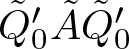 $\tilde Q_0'\tilde A\tilde Q_0'$ in the range of
 $\tilde Q_0'$. That is,
 $\alpha=0$ and
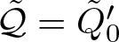 $\tilde{\mathcal{Q}}=\tilde Q_0'$.
The eigenprojection of  $\tilde B$ corresponding to
 $\sigma_i'$,
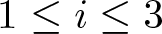 $1\le i\le3$, are
 \begin{equation*}
\begin{aligned}
&\tilde Q_1'=\tilde w_w(0,1,0,0)^t(0,1,0,0)w_{\tilde w},\\
&\tilde Q_2'=\tilde w_w(0,0,1,0)^t(-\frac32R\bar T_1,0,1,-\frac D2R)w_{\tilde w},\\
&\tilde Q_3'=\tilde w_w(0,0,\frac{DR}2,1)^t(-\bar T_1,0,0,1)w_{\tilde w},
\end{aligned}
\end{equation*}
and
 \begin{equation}
\tilde S'=\frac{\bar\rho}{\bar\mu_{\rm tr}}\tilde Q_1'+\frac{3R\bar\rho}{2\bar\lambda_{\rm tr}}\tilde Q_2'+\frac{5R\bar\rho}{2\bar\lambda_{\rm tr}}\tilde Q_3'.
\end{equation}
Thus, applying (5.67), (5.57)-(5.59) and (5.68), and by direct calculation,
 \begin{equation*}
\begin{aligned}
&\tilde{\mathcal{Q}}\tilde A\tilde S'\tilde A\tilde{\mathcal{Q}}=\tilde Q_0'\tilde A\tilde S'\tilde A\tilde Q_0'=\frac{\bar\rho}{\bar\mu_{\rm tr}}a_{23}\frac{3+D}2R\bar T_1\tilde Q_0'=\frac{\bar\rho}{\bar\mu_{\rm tr}}R\bar T_1\tilde Q_0',\\
&\tilde{\mathcal{Q}}\tilde L\tilde{\mathcal{Q}}=\tilde Q_0'\mbox{diag}(0,0,0,k_4)\tilde Q_0'=0.
\end{aligned}
\end{equation*}
These give us
 \begin{equation*}
\tilde{\mathcal{Q}}(\tilde A\tilde S'\tilde A-\tilde L)\tilde{\mathcal{Q}}=\frac{\bar\rho R\bar T_1}{\bar\mu_{\rm tr}}\tilde Q_0',
\end{equation*}
where the right-hand side is the spectral decomposition of the matrix on the left-hand side in the range of 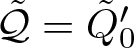 $\tilde{\mathcal{Q}}=\tilde Q_0'$. Therefore,
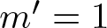 $m'=1$,
 \begin{equation*}
\beta=\frac{\bar\rho R\bar T_1}{\bar\mu_{\rm tr}} \gt 0,
\end{equation*}
and 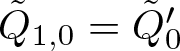 $\tilde Q_{1,0}=\tilde Q_0'$. To go back to the original variable
 $w$ we set
 \begin{equation}
Q_{1,0}=w_{\tilde w}\tilde Q_0'\tilde w_w=\begin{pmatrix}1\\0\\ \frac{3+D}2R\bar T_1\\ \bar T_1\end{pmatrix}(1,0,0,0).
\end{equation}
Gathering the information obtained above, we formulate the Green’s function for the Cauchy problem of (5.53), (5.54) as follows,
 \begin{align}
G(x,t)=& H(x,t;-\bar c,\mu_-)P_-+H(x,t;0,\mu_0)P_0+H(x,t;\bar c,\mu_+)P_+\nonumber\\
& +O(1)(t+1)^{-\frac12}[H(x,t;-\bar c,C)+H(x,t;0,C)+H(x,t;\bar c,C)] \nonumber\\
& +e^{-\beta t}\delta(x)Q_{1,0},
\end{align}
where
 \begin{equation}
\begin{aligned}
&\bar c=\sqrt{\frac{5+D}{3+D}R\bar T_1},\qquad \mu_0=\frac{2\bar\lambda_{\rm tr}}{5R\bar\rho},\\
&\mu_{\pm}=\frac{DR\bar T_1}{3(3+D)\theta A_c(\bar T_1)\bar\rho}+\frac{\bar\mu_{\rm tr}}{2\bar\rho}+\frac{2\bar\lambda_{\rm tr}}{5(3+D)R\bar\rho},\qquad
\beta=\frac{R\bar T_1\bar\rho}{\bar\mu_{\rm tr}},
\end{aligned}
\end{equation}
 $C \gt 0$ is a constant, and the projections
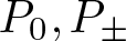 $P_0,P_{\pm}$ and
 $Q_{1,0}$ are given in (5.62), (5.63) and (5.69).
We comment that while the setup of the two-temperature Navier–Stokes type model (1.9) is different from that of the thermal nonequilibrium flow model (1.4), the two systems have similar structure. In particular, the linearized system (5.53), (5.54) is parallel to (5.6), (5.8). Indeed, if we symbolically make the following correspondence between the two systems,
 \begin{equation*}
\bar\mu\longleftrightarrow\bar\mu_{\rm tr}, \qquad\bar\kappa\longleftrightarrow\bar\lambda_{\rm tr},\qquad
\bar\nu\longleftrightarrow\frac{2\bar\lambda_{\rm tr}}{5R\bar\rho},\qquad\bar\tau\longleftrightarrow\frac{3+D}{3\theta A_c(\bar T_1)\bar\rho},
\end{equation*}
together with (1.10) and (1.12), we can derive the same formulation in (5.71) from (5.16), (5.29),(5.31) and (5.40).
Data availability statement
My manuscript has no associated data.
Acknowledgements
The author would like to thank the anonymous referee for constructive comments and suggestions, which helped improve the quality of the paper.
Funding statement
This work was supported by the National Science Foundation under grant DMS-1908195.
Appendix A. Alternative steps for procedure 2.9
If  $A^{(r)}$ defined in (2.19) has multiple eigenvalues, we modify Steps 1 and 2 of Procedure 2.9 to Steps 1
 $'$ and 2
 $'$ as follows.
Step 1 $'$. Let
 $\lambda^{(r)}_1 \lt \lambda^{(r)}_2 \lt \cdots \lt \lambda^{(r)}_{\tilde s}$ be distinct eigenvalues of
 $A^{(r)}$. Find the spectral decomposition
 \begin{equation}
A^{(r)}=\sum_{k=1}^{\tilde s} \lambda^{(r)}_kP^{(r)}_k,
\end{equation}
where  $P^{(r)}_k$,
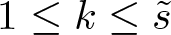 $1\le k\le\tilde s$, is the eigenprojection of
 $A^{(r)}$ corresponding to
 $\lambda^{(r)}_k$.
Step 2 $'$. Find the spectral decomposition of
 $L$,
 \begin{equation}
L=\sum^s_{j=1}-\sigma_jQ_j,
\end{equation}
with 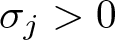 $\sigma_j \gt 0$,
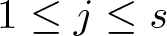 $1\le j\le s$. Here each
 $-\sigma_j$ is a negative eigenvalue of
 $L$, with the corresponding eigenprojection
 $Q_j$. Let
 $Q_0$ be the eigenprojection of
 $L$ corresponding to the eigenvalue zero,
 \begin{equation}
Q_0=\operatorname{diag}(I_{n_1\times n_1}, 0_{n_2\times n_2}).
\end{equation}
Define
 \begin{equation}
S=\sum_{j=1}^s\frac1{\sigma_j}Q_j,
\end{equation}
which is the value at zero of the reduced resolvent of  $-L$ with respect to the eigenvalue zero.
Now for each  $P^{(r)}_k$ associated with a distinct
 $\lambda^{(r)}_k$ in (A.1), we form a matrix
 $\operatorname{diag}(P^{(r)}_k,0_{n_2\times n_2})(ASA+B)\operatorname{diag}(P^{(r)}_k,0_{n_2\times n_2})$ and find its spectral decomposition in the range of
 $\operatorname{diag}(P^{(r)}_k,0_{n_2\times n_2})$,
 \begin{equation}
\begin{aligned}
&\operatorname{diag}(P^{(r)}_k,0_{n_2\times n_2})(ASA+B)\operatorname{diag}(P^{(r)}_k,0_{n_2\times n_2})=\sum_{k'=1}^{\tilde s_k}\mu_{kk'}P_{kk'},\\
&\sum_{k'=1}^{\tilde s_k}P_{kk'}=\operatorname{diag}(P^{(r)}_k,0_{n_2\times n_2}).
\end{aligned}
\end{equation}
Next, we collect all distinct pairs 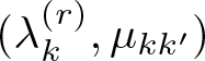 $(\lambda^{(r)}_k,\mu_{kk'})$,
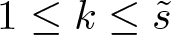 $1\le k\le \tilde s$,
 $1\le k'\le\tilde s_k$. The total number of those pairs is
 $m$ in th first term of (2.5), with
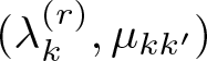 $(\lambda^{(r)}_k,\mu_{kk'})$ being
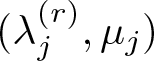 $(\lambda^{(r)}_j,\mu_j)$ and
 $P_{kk'}$ being
 $P_j$ therein.
After Steps 1 $'$ and 2
 $'$, one continues with Steps 3 and 4 in Procedure 2.9.
In case  $\alpha_k$,
 $1\le k\le s^{\prime\prime}$, in (2.27) are simple, we simplify Step 4 in Procedure 2.9 to Step 4
 $'$ as follows. This is regardless of using Steps 1 and 2 or Steps 1
 $'$ and 2
 $'$.
Step 4 $'$. If all
 $\alpha_k$ is (2.27) are simple, i.e., all
 $\mathcal{Q}_k$ are rank one, then
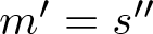 $m'=s^{\prime\prime}$ is the rank of
 $Q'_0$. Let the normalized left eigenvector (row vector) and right eigenvector of
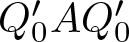 $Q'_0AQ'_0$ associated with
 $\alpha_j$ be
 $l'_j$ and
 $r'_j$, respectively,
 \begin{gather*}
Q'_0AQ'_0r'_j=\alpha_jr'_j,\qquad l'_jQ'_0AQ'_0=\alpha_jl'_j,\qquad1\le j\le m',\\
l'_ir'_j=\delta_{ij},\qquad 1\le i,j\le m'.
\end{gather*}
For each  $\alpha_j$ in the third term of (2.5), the corresponding
 $\beta_j$ and
 $Q_{j,0}$ are
 \begin{equation}
\beta_j=l'_j(AS'A-L)r'_j,\qquad Q_{j,0}=r'_jl'_j=\mathcal{Q}_j,
\end{equation}
where  $S'$ is defined by (2.28).


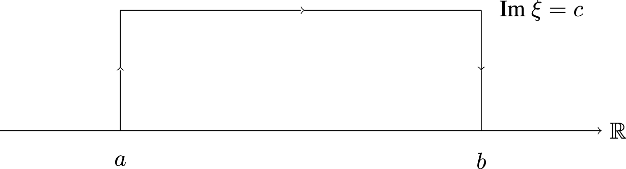

 Open access

