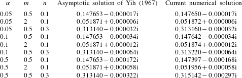
1 Introduction
The stability of two-layer fluid flows plays an important role in the behaviour of many natural phenomena, such as flows of magma, glaciers, the Earth’s outer core, ocean and atmosphere, as well as in many industrial applications, such as oil extraction, recovery and transportation (Saffman & Taylor Reference Saffman and Taylor1958; Joseph et al. Reference Joseph, Bai, Chen and Renardy1997), coating technology (Weinstein & Ruschak Reference Weinstein and Ruschak2004), co-extrusion of two molten polymers (Schrenk & Alfrey Reference Schrenk, Alfrey, Paul and Newman1978), displacement flow (Redapangu, Sahu & Vanka Reference Redapangu, Sahu and Vanka2013) and de-icing of airplane wings (Yih Reference Yih1990). A number of reviews have addressed the general mathematical theory and applications of two-fluid systems (Joseph & Renardy Reference Joseph and Renardy1993), the dynamics of thin liquid films (Craster & Matar Reference Craster and Matar2009), the physical mechanisms by which viscosity variations influence the flow stability (Govindarajan & Sahu Reference Govindarajan and Sahu2014), the stability of two-fluid boundary layers (Timoshin Reference Timoshin1997; Özgen, Degrez & Sarma Reference Özgen, Degrez and Sarma1998; Timoshin & Hooper Reference Timoshin and Hooper2000) and the stability of two-fluid parallel flows (Mohammadi & Smits Reference Mohammadi and Smits2016).
Two-fluid systems have received increased attention recently because of their relevance to understanding the drag reduction potential of superhydrophobic surfaces (SHS) (Rothstein Reference Rothstein2010; Busse et al. Reference Busse, Sandham, McHale and Newton2013) and liquid-infused surfaces (LIS) (Wong et al. Reference Wong, Kang, Tang, Smythe, Hatton, Grinthal and Aizenberg2011; Solomon, Khalil & Varanasi Reference Solomon, Khalil and Varanasi2014; Rosenberg et al. Reference Rosenberg, Van Buren, Fu and Smits2016). One of the principal challenges in these applications is maintaining the robustness and longevity of the interface between the water and air (SHS), or between the water and infused liquid (LIS). Such systems are susceptible to different failure mechanisms, including pressure-induced drainage, shear-induced drainage and gravity-induced drainage (Jacobi, Wexler & Stone Reference Jacobi, Wexler and Stone2015; Wexler et al. Reference Wexler, Grosskopf, Chow, Fan, Jacobi and Stone2015a ; Wexler, Jacobi & Stone Reference Wexler, Jacobi and Stone2015b ). Both SHS and LIS may also fail due to the presence of interfacial instabilities, and it is this particular failure mode that is the principal motivation for the current effort.
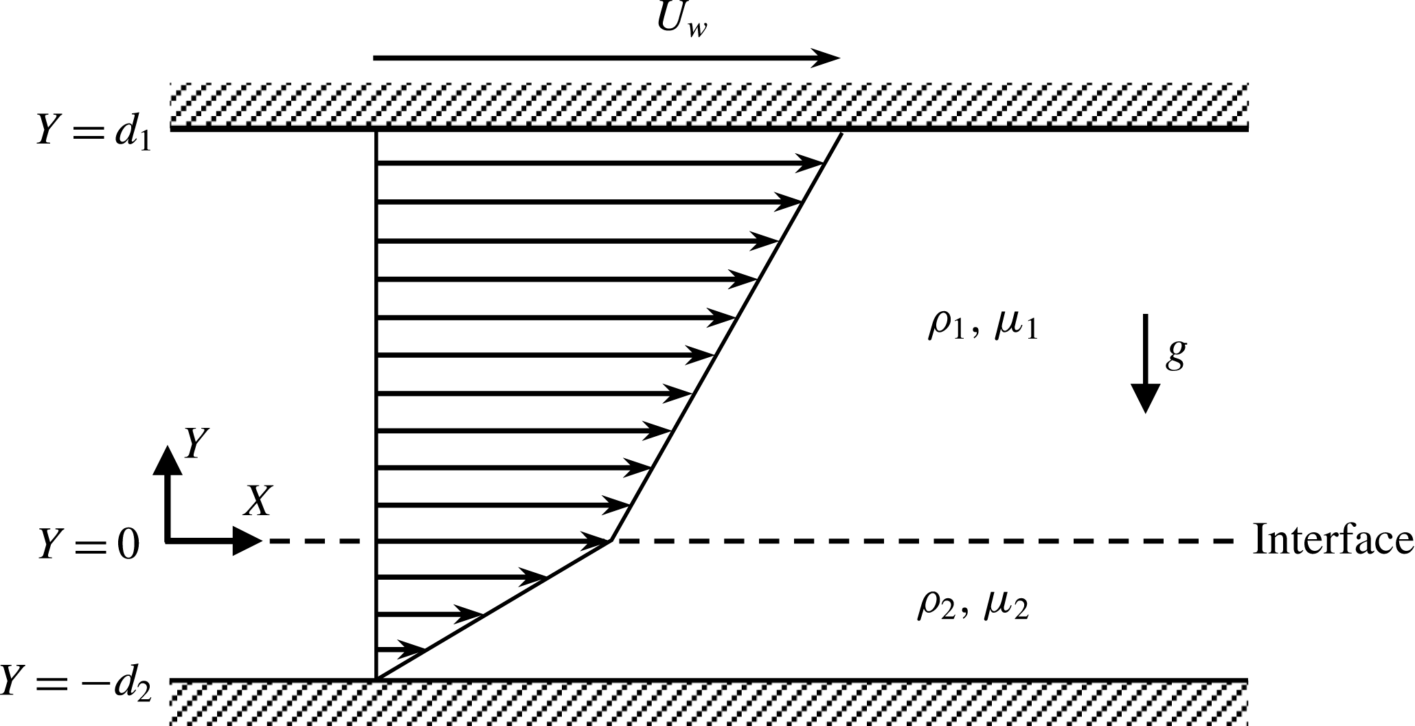
Sketch of the flow configuration, where
 $g$
is the acceleration due to gravity. Other parameters are defined in the text.

To better understand these failure modes, we focus on the linear stability analysis of two-layer Couette flow. Plane, single-layer Couette flow is known to be linearly stable for all values of Reynolds number (Schmid & Henningson Reference Schmid and Henningson2001). This is not true for two-layer systems. The stability of two-layer Couette flow in a channel (see figure 1) is governed by the density ratio (
 $r:=\unicode[STIX]{x1D70C}_{2}/\unicode[STIX]{x1D70C}_{1}$
), dynamic viscosity ratio (
 $m:=\unicode[STIX]{x1D707}_{2}/\unicode[STIX]{x1D707}_{1}$
), thickness ratio (
 $n:=d_{2}/d_{1}$
), inverse Froude number (
 $F$
), inverse Weber number (
 $\unicode[STIX]{x1D6E4}$
), Reynolds number (
 $Re$
) and the disturbance wavenumbers in the streamwise (
 $\unicode[STIX]{x1D6FC}$
) and spanwise (
 $\unicode[STIX]{x1D6FD}$
) directions. Here,
 $\unicode[STIX]{x1D70C}_{j}$
,
 $\unicode[STIX]{x1D707}_{j}$
and
 $d_{j}$
denote density, dynamic viscosity and thickness of fluid
 $j$
, respectively, where
 $j=1$
(upper fluid) or 2 (lower fluid). Definitions of the remaining parameters are given in § 2. Note that the stability of a single-fluid flow is described by only three parameters (
 $\unicode[STIX]{x1D6FC}$
,
 $\unicode[STIX]{x1D6FD}$
and
 $Re$
), but by adding the second layer of fluid five additional parameters (
 $r$
,
 $m$
,
 $n$
,
 $F$
and
 $\unicode[STIX]{x1D6E4}$
) appear, as given by Hooper (Reference Hooper1985) and Yiantsios & Higgins (Reference Yiantsios and Higgins1988).
Linear stability of two-layer fluid flows was first investigated by Yih (Reference Yih1963, Reference Yih1967), who obtained the complex wave speed in the limit of long-wavelength disturbances using the method of non-singular perturbation. Yih demonstrated that, for both plane Couette and Poiseuille flows, viscosity stratification can give rise to a new type of disturbance called the interfacial mode, which occurs near the interface and grows relatively faster in the less viscous fluid layer. Yih (Reference Yih1967) showed that the flow is unstable when the thickness of the more viscous fluid is smaller than the thickness of the less viscous fluid, and found that the rate of growth of the instability is
 $O(\unicode[STIX]{x1D6FC}^{2})$
. His analysis also showed that the flow is neutrally stable for
 $m=1$
and for all values of
 $n$
, and that for
 $n>2.5$
the interfacial mode stabilizes for all values of
 $m$
above 1 at least up to
 $m=70$
.
Hooper & Boyd (Reference Hooper and Boyd1983) investigated the linear stability of the concurrent flow of two superposed immiscible viscous fluids, each in uniform shearing motion in an unbounded domain. They derived analytical expressions for the complex phase speed of the short-wavelength and long-wavelength instabilities for two special cases: (i) fluids with
 $r=1$
,
 $\unicode[STIX]{x1D6E4}=0$
and different viscosities, and (ii) fluids with
 $r\neq 1$
,
 $\unicode[STIX]{x1D6E4}\neq 0$
and different viscosities. In case (i), they found that the flow is always unstable in the absence of interfacial tension in the limit of short-wavelength disturbances. In case (ii), increasing the interfacial tension always resulted in stabilization, whereas density stratification can either stabilize or destabilize the flow. When the lower fluid is the less viscous one (
 $m<1$
), the density difference has a destabilizing effect if the lower fluid is the more dense one (
 $r>1$
), and it has a stabilizing effect if the lower fluid is the less dense one (
 $r<1$
). The density difference has the opposite effect when
 $m>1$
. They did not find any instability in the limit of long-wavelength disturbances, and showed that these waves decay at the rate of
 $O(\unicode[STIX]{x1D6FC}^{2})$
. By analysing the energy equation for the unstable mode, they discovered that the instability is created in the vicinity of the interface in the fluid with the smaller viscosity, regardless of whether the less viscous fluid occupies the upper or the lower layer. The growth rate of the disturbances is very sensitive even to small values of interfacial tension but it is always slow, helping to explain why these disturbances have not been observed experimentally.
Hinch (Reference Hinch1984) discovered the mechanism driving the short-wave instability found by Hooper & Boyd (Reference Hooper and Boyd1983). Because the basic flow velocities are discontinuous at the perturbed interface, the disturbance velocities must be generated so as to compensate for the difference in velocities. The resulting disturbance vorticities that are initially in phase with the interface are advected by the basic flow and so slight out-of-phase components occur. These out-of-phase components create flow disturbances that can amplify the initial perturbation of the interface and cause the instability to develop.
Hooper (Reference Hooper1985) further studied these instabilities using long-wavelength perturbation analysis in a configuration where a thin layer of fluid is bounded from below by a solid wall moving at a constant speed
 $U_{0}$
, and an infinitely deep second fluid overlies the thin layer. Hooper showed that there are an infinite number of modes that govern the stability of this flow. Among all these modes, only one mode becomes unstable when the viscosity of the thin layer is greater than the viscosity of the overlying layer. The behaviour of the stable modes in the limit of long wavelength seems to be similar to the behaviour of the stable modes found in the case of single-fluid, semi-infinite Couette flow bounded by one wall. That is, long-wavelength modes are insensitive to the presence of the thin layer of fluid, and to these modes the thin layer just appears to be an extension of the solid wall.
The cases studied by Yih (Reference Yih1967), Hooper & Boyd (Reference Hooper and Boyd1983) and Hooper (Reference Hooper1985) demonstrate that the presence of at least one solid wall is sufficient for two-layer Couette flow to become unstable to a long-wave instability. The rate of growth of the disturbances, however, changes: for flow bounded by only one wall, it is
 $O(\unicode[STIX]{x1D6FC}^{4/3})$
, faster than in the case of two-layer Couette flow in a channel, where they grow at a rate
 $O(\unicode[STIX]{x1D6FC}^{2})$
(Yih Reference Yih1967). That is, adding a second wall has a stabilizing effect for the long-wavelength disturbances. The velocity field is always destabilizing because the disturbance vorticity in the upper fluid layer becomes out of phase with respect to the disturbance vorticity in the lower fluid layer as the flow is driven by the main shear.
Charru & Hinch (Reference Charru and Hinch2000) provided a unified view of the physical mechanisms responsible for the appearance of different types of instabilities in two-fluid Couette flows by means of a phase diagram, in essence a generalization of the flow regimes defined by Hooper & Boyd (Reference Hooper and Boyd1987). Charru & Hinch (Reference Charru and Hinch2000) constructed this view in analogy with single-fluid Couette flow over a wavy wall, which depends on only two parameters: (i) the dimensionless thickness (non-dimensionalized by the inverse wavenumber of the wavy wall), and (ii) a viscous diffusion length. Based on these parameters, three flow regimes emerge – the shallow viscous regime, the deep viscous regime, and the inviscid regime, characterized by an effective Reynolds number and a penetration depth defined for the vorticity disturbances. Charru & Hinch (Reference Charru and Hinch2000) showed that, for the case where interfacial tension and gravity are ignored, the problem of two-fluid Couette flow depends only on four parameters: the dimensionless thickness and viscous length for each layer of fluid. Similar flow regimes can be identified. A typical example of the shallow viscous regime is the long-wave disturbances discovered by Yih (Reference Yih1967), whereas the short-wave disturbances discovered by Hooper & Boyd (Reference Hooper and Boyd1983) belong to the deep viscous regime. For the inviscid regime corresponding to strong shear rates (large values of shear rate or small values of viscous length), there is no evidence for the interfacial instability, but this condition may give rise to a wall mode instability (Tollmien–Schlichting or TS wave).
Finally, Barthelet, Charru & Fabre (Reference Barthelet, Charru and Fabre1995) investigated the interfacial long-wave instability of double-layer Couette flow experimentally in a channel bent into an annular ring. This configuration enabled them to observe the wave evolution over very long periods of time and it also yielded a discrete wavenumber spectrum. Depending on the thickness ratio
 $n$
and the viscosity ratio
 $m$
, long-wave instabilities were observed with a wavelength equal to the perimeter of the test channel, while the critical values for the velocity of the upper plate were approximately three times smaller than the long-wavelength asymptotic solution given by Yih (Reference Yih1967). They argued that the differences between experiment and theory may be due to centrifugal effects (caused by the channel curvature modifying the base flow profile from Couette flow) and possibly the destabilizing effects of the secondary flow.
Almost all of the theoretical or numerical studies discussed above were limited to either short-wavelength or long-wavelength approximations, and for most cases either the density contrast or the interfacial tension were ignored. The experimental studies sometimes contradict each other or disagree at some level with the theoretical work. To better illuminate the full complexity of this problem, which is governed by a large number of parameters, we provide a spectral formulation for the linear stability of two-layer Couette flows and systematically address how the flow stability is affected by the full set of governing parameters.
2 Problem formulation
Consider fully developed Couette flow of two immiscible fluids between two parallel plates, as shown in figure 1. The problem can be non-dimensionalized using the half channel height
 $L=(d_{1}+d_{2})/2$
, the velocity of the upper plate
 $U_{w}$
and the reference pressure
 $\unicode[STIX]{x1D70C}_{1}U_{w}^{2}$
. The basic flow takes the form
 $$\begin{eqnarray}\displaystyle \displaystyle U_{1}(y) & = & \displaystyle A_{1}+B_{1}y,\quad 0\leqslant y\leqslant y_{U},\end{eqnarray}$$
 $$\begin{eqnarray}\displaystyle \displaystyle U_{2}(y) & = & \displaystyle A_{2}+B_{2}y,\quad y_{L}\leqslant y\leqslant 0,\end{eqnarray}$$
 $y=Y/L$
,
 $y_{U}=d_{1}/L=2/(1+n)$
and
 $y_{L}=-d_{2}/L=-2n/(1+n)$
. Coefficients
 $A_{j}$
and
 $B_{j}$
(
 $j=1,2$
) are determined by applying the boundary conditions at the walls and the continuity of velocity and shear stress at the interface, namely
 $$\begin{eqnarray}\displaystyle & \displaystyle U_{1}(y_{U})=1, & \displaystyle\end{eqnarray}$$
 $$\begin{eqnarray}\displaystyle & \displaystyle U_{2}(y_{L})=0, & \displaystyle\end{eqnarray}$$
 $$\begin{eqnarray}\displaystyle & \displaystyle U_{1}(0)=U_{2}(0), & \displaystyle\end{eqnarray}$$
 $$\begin{eqnarray}\displaystyle & \displaystyle \text{D}U_{1}(0)=m\text{D}U_{2}(0), & \displaystyle\end{eqnarray}$$
 $\text{D}=\text{d}/\text{d}y$
. Solutions of (2.2) give
 $A_{1}=A_{2}=n/(m+n)$
,
 $B_{1}=m(1+n)/[2(m+n)]$
and
 $B_{2}=B_{1}/m$
. The average velocity in each layer takes the form
 $$\begin{eqnarray}\displaystyle & \displaystyle U_{1,a}=\frac{\displaystyle \int _{0}^{y_{U}}U_{1}(y)\,\text{d}y}{\displaystyle \int _{0}^{y_{U}}\text{d}y}=\frac{m+2n}{2(m+n)}, & \displaystyle\end{eqnarray}$$
 $$\begin{eqnarray}\displaystyle & \displaystyle U_{2,a}=\frac{\displaystyle \int _{y_{L}}^{0}U_{2}(y)\,\text{d}y}{\displaystyle \int _{y_{L}}^{0}\text{d}y}=\frac{n}{2(m+n)}. & \displaystyle\end{eqnarray}$$
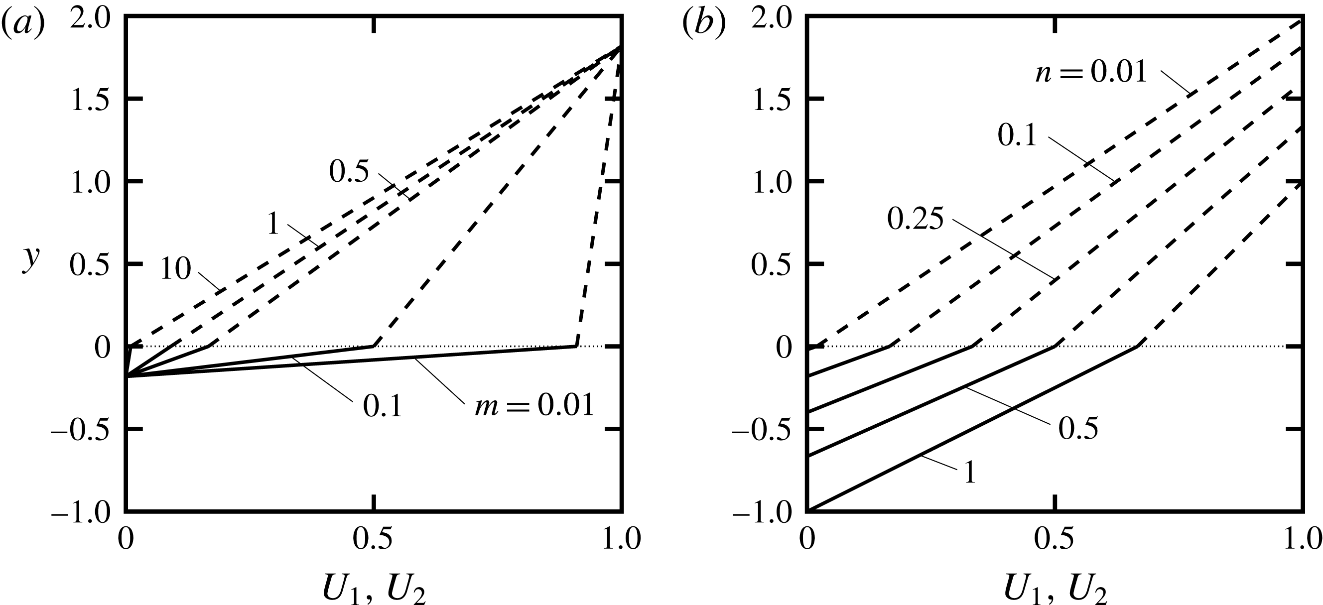
 $n=0.1$
. As the viscosity ratio
 $m$
increases, the interface velocity decreases, and the slope of the velocity profile in the upper layer increases while the slope of the velocity profile in the lower layer decreases.
Base flow velocity profiles for two-layer Couette flow: (a)
 $n=0.1$
and different
 $m$
; (b)
 $m=0.5$
and different
 $n$
. Dashed, solid and dotted lines denote
 $U_{1}$
,
 $U_{2}$
and the location of the interface, respectively.

Figure 2(b) shows the effect of thickness ratio
 $n$
on velocity profiles for the case where
 $m=0.5$
. The ratio of the slope of the upper velocity profile to the slope of the lower one is always
 $m$
(2.1), that is,
 $B_{1}/B_{2}=0.5$
. As
 $n$
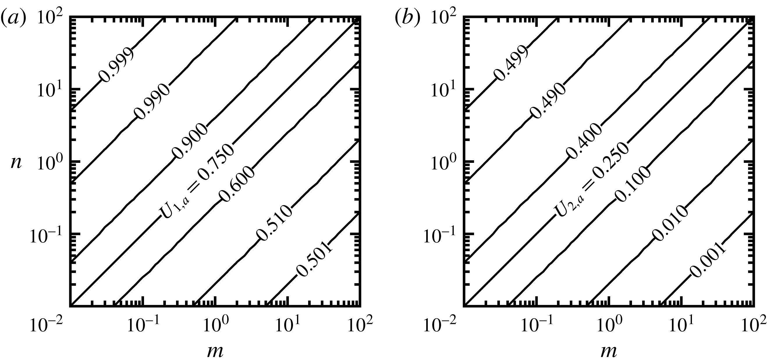
increases, the slopes of the upper and lower velocity profiles decrease. Note that the total channel height is always equal to 2, so that the difference between the highest and lowest points on each curve in figure 2(a,b) is always 2. The average velocities computed from (2.3) and shown in figure 3 indicate that, as
 $n$
increases for a fixed
 $m$
, the average velocity increases in both layers. Figure 3 also shows that, for a fixed
 $n$
, increasing
 $m$
leads to decrease in the average velocities. The limiting cases for average velocities can be found from (2.3), and take the form
 $$\begin{eqnarray}\displaystyle & \displaystyle \lim _{m\rightarrow 0}U_{1,a}=\lim _{n\rightarrow \infty }U_{1,a}=1, & \displaystyle\end{eqnarray}$$
 $$\begin{eqnarray}\displaystyle & \displaystyle \lim _{m\rightarrow n}U_{1,a}=0.75, & \displaystyle\end{eqnarray}$$
 $$\begin{eqnarray}\displaystyle & \displaystyle \lim _{m\rightarrow \infty }U_{1,a}=\lim _{n\rightarrow 0}U_{1,a}=0.5, & \displaystyle\end{eqnarray}$$
 $$\begin{eqnarray}\displaystyle & \displaystyle \lim _{m\rightarrow 0}U_{2,a}=\lim _{n\rightarrow \infty }U_{2,a}=0.5, & \displaystyle\end{eqnarray}$$
 $$\begin{eqnarray}\displaystyle & \displaystyle \lim _{m\rightarrow n}U_{2,a}=0.25, & \displaystyle\end{eqnarray}$$
 $$\begin{eqnarray}\displaystyle & \displaystyle \lim _{m\rightarrow \infty }U_{2,a}=\lim _{n\rightarrow 0}U_{2,a}=0. & \displaystyle\end{eqnarray}$$
Average velocities of basic flows for (a) upper layer
 $U_{1,a}$
, and (b) lower layer
 $U_{2,a}$
computed from (2.3).

The governing equations for the (three-dimensional) stability problem are the continuity and the linearized Navier–Stokes equations, which reduce to a set of Orr–Sommerfeld (normal velocity) and Squire (normal vorticity) equations for each layer of the two fluids. That is,
 $$\begin{eqnarray}\displaystyle & \displaystyle \left[\frac{\text{i}}{Re}\left(\text{D}^{2}-k^{2}\right)^{2}+\unicode[STIX]{x1D6FC}\left(U_{1}\text{D}^{2}-\text{D}^{2}U_{1}-k^{2}U_{1}\right)\right]v_{1}=\unicode[STIX]{x1D70E}(\text{D}^{2}-k^{2})v_{1}, & \displaystyle\end{eqnarray}$$
 $$\begin{eqnarray}\displaystyle & \displaystyle \left(\unicode[STIX]{x1D6FD}\text{D}U_{1}\right)v_{1}+\left[\frac{\text{i}}{Re}\left(\text{D}^{2}-k^{2}\right)+\unicode[STIX]{x1D6FC}U_{1}\right]\unicode[STIX]{x1D702}_{1}=\unicode[STIX]{x1D70E}\unicode[STIX]{x1D702}_{1}, & \displaystyle\end{eqnarray}$$
 $$\begin{eqnarray}\displaystyle & \displaystyle \left[\frac{\text{i}m}{Re}\left(\text{D}^{2}-k^{2}\right)^{2}+r\unicode[STIX]{x1D6FC}\left(U_{2}\text{D}^{2}-\text{D}^{2}U_{2}-k^{2}U_{2}\right)\right]v_{2}=\unicode[STIX]{x1D70E}[r(\text{D}^{2}-k^{2})]v_{2}, & \displaystyle\end{eqnarray}$$
 $$\begin{eqnarray}\displaystyle & \displaystyle \left(r\unicode[STIX]{x1D6FD}\text{D}U_{2}\right)v_{2}+\left[\frac{\text{i}m}{Re}\left(\text{D}^{2}-k^{2}\right)+r\unicode[STIX]{x1D6FC}U_{2}\right]\unicode[STIX]{x1D702}_{2}=\unicode[STIX]{x1D70E}r\unicode[STIX]{x1D702}_{2}, & \displaystyle \displaystyle\end{eqnarray}$$
 $$\begin{eqnarray}\displaystyle \displaystyle v_{j}^{\prime }(x,y,z,t) & = & \displaystyle v_{j}(y)\text{e}^{\text{i}(\unicode[STIX]{x1D6FC}x+\unicode[STIX]{x1D6FD}z-\unicode[STIX]{x1D70E}t)},\end{eqnarray}$$
 $$\begin{eqnarray}\displaystyle \displaystyle \unicode[STIX]{x1D702}_{j}^{\prime }(x,y,z,t) & = & \displaystyle \unicode[STIX]{x1D702}_{j}(y)\text{e}^{\text{i}(\unicode[STIX]{x1D6FC}x+\unicode[STIX]{x1D6FD}z-\unicode[STIX]{x1D70E}t)}.\end{eqnarray}$$
 $Re:=\unicode[STIX]{x1D70C}_{1}U_{w}d_{1}(1+n)/(2\unicode[STIX]{x1D707}_{1})$
is the Reynolds number,
 $\unicode[STIX]{x1D70E}=\unicode[STIX]{x1D70E}_{r}+\text{i}\unicode[STIX]{x1D70E}_{i}$
is the complex amplification rate,
 $\unicode[STIX]{x1D70E}_{r}$
is the angular frequency,
 $\unicode[STIX]{x1D70E}_{i}$
is the growth rate of disturbances,
 $c=\unicode[STIX]{x1D70E}/\unicode[STIX]{x1D6FC}$
is the complex phase speed,
 $v_{j}$
and
 $\unicode[STIX]{x1D702}_{j}$
(
 $j=1,2$
) denote eigenfunctions describing disturbance normal velocities (
 $v_{j}^{\prime }$
) and disturbance normal vorticities (
 $\unicode[STIX]{x1D702}_{j}^{\prime }$
), respectively,
 $\unicode[STIX]{x1D6FC}$
and
 $\unicode[STIX]{x1D6FD}$
are the disturbance wavenumbers in the x- and z-directions, respectively, and
 $k=\sqrt{\unicode[STIX]{x1D6FC}^{2}+\unicode[STIX]{x1D6FD}^{2}}$
.
Equations (2.5a )–(2.5d ) require a total of twelve boundary conditions. The no-slip and no-penetration conditions at the walls provide six conditions, given by
 $$\begin{eqnarray}\displaystyle & \displaystyle v_{1}(y_{U})=0, & \displaystyle\end{eqnarray}$$
 $$\begin{eqnarray}\displaystyle & \displaystyle \text{D}v_{1}(y_{U})=0, & \displaystyle\end{eqnarray}$$
 $$\begin{eqnarray}\displaystyle & \displaystyle \unicode[STIX]{x1D702}_{1}(y_{U})=0, & \displaystyle\end{eqnarray}$$
 $$\begin{eqnarray}\displaystyle & \displaystyle v_{2}(y_{L})=0, & \displaystyle\end{eqnarray}$$
 $$\begin{eqnarray}\displaystyle & \displaystyle \text{D}v_{2}(y_{L})=0, & \displaystyle\end{eqnarray}$$
 $$\begin{eqnarray}\displaystyle & \displaystyle \unicode[STIX]{x1D702}_{2}(y_{L})=0. & \displaystyle\end{eqnarray}$$
 $$\begin{eqnarray}\displaystyle & \displaystyle v_{1}(0)-v_{2}(0)=0, & \displaystyle\end{eqnarray}$$
 $$\begin{eqnarray}\displaystyle & \displaystyle \text{D}v_{1}(0)-\text{D}v_{2}(0)-\text{i}\unicode[STIX]{x1D6FC}\left[\text{D}U_{1}(0)-\text{D}U_{2}(0)\right]H=0, & \displaystyle\end{eqnarray}$$
 $$\begin{eqnarray}\displaystyle & \displaystyle \unicode[STIX]{x1D702}_{1}(0)-\unicode[STIX]{x1D702}_{2}(0)+\text{i}\unicode[STIX]{x1D6FD}\left[\text{D}U_{1}(0)-\text{D}U_{2}(0)\right]H=0, & \displaystyle\end{eqnarray}$$
 $$\begin{eqnarray}\displaystyle & \displaystyle \left(\text{D}^{2}+k^{2}\right)v_{1}(0)-m\left(\text{D}^{2}+k^{2}\right)v_{2}(0)=0, & \displaystyle\end{eqnarray}$$
 $$\begin{eqnarray}\displaystyle & \displaystyle \text{D}\unicode[STIX]{x1D702}_{1}(0)-m\text{D}\unicode[STIX]{x1D702}_{2}(0)=0, & \displaystyle\end{eqnarray}$$
 $$\begin{eqnarray}\displaystyle & & \displaystyle \{\text{D}^{3}-3k^{2}\text{D}+\text{i}\unicode[STIX]{x1D6FC}Re(r-1)[U_{1}(0)\text{D}-\text{D}U_{1}(0)]\}v_{1}(0)\nonumber\\ \displaystyle & & \displaystyle \qquad \quad -\,m(\text{D}^{3}-3k^{2}\text{D})v_{2}(0)+k^{2}Re(F+k^{2}\unicode[STIX]{x1D6E4})H=\unicode[STIX]{x1D70E}[\text{i}Re(r-1)\text{D}]v_{1}(0),\quad\end{eqnarray}$$
 $F:=(r-1)gd_{1}(1+n)/(2U_{w}^{2})$
is an inverse Froude number, g is the gravitational acceleration,
 $\unicode[STIX]{x1D6E4}:=2\unicode[STIX]{x1D6FE}/[\unicode[STIX]{x1D70C}_{1}d_{1}(1+n)U_{w}^{2}]$
is an inverse Weber number and
 $\unicode[STIX]{x1D6FE}$
is the interfacial tension. The kinematic condition at the interface takes the form
 $$\begin{eqnarray}\text{i}v_{1}(0)+[\unicode[STIX]{x1D6FC}U_{1}(0)]H=\unicode[STIX]{x1D70E}H,\end{eqnarray}$$
where H is the amplitude of the perturbed interface, which has a position h given by
 $$\begin{eqnarray}h(x,z,t)=H\text{e}^{\text{i}(\unicode[STIX]{x1D6FC}x+\unicode[STIX]{x1D6FD}z-\unicode[STIX]{x1D70E}t)}.\end{eqnarray}$$
Equations (2.5), along with boundary conditions (2.7) and (2.8), and the kinematic condition (2.9), construct a generalized eigenvalue problem of the form
 $$\begin{eqnarray}A\unicode[STIX]{x1D6F7}=\unicode[STIX]{x1D70E}B\unicode[STIX]{x1D6F7},\quad \unicode[STIX]{x1D6F7}=\{v_{1},\unicode[STIX]{x1D702}_{1},v_{2},\unicode[STIX]{x1D702}_{2},H\}.\end{eqnarray}$$
The parameter
 $H$
could be replaced with the help of (2.9), but it is essential for the construction of the generalized eigenvalue problem (2.11), and thereby allows the computation of the full spectrum of solutions for any combination of parameters. The other advantage of introducing
 $H$
, as noted by Malik & Hooper (Reference Malik and Hooper2007), is to achieve more accurate results for the eigenvalues
 $\unicode[STIX]{x1D70E}$
and the eigenfunctions
 $\unicode[STIX]{x1D6F7}$
.
The goal in linear stability analysis is to find the dispersion relation
 $\unicode[STIX]{x1D70E}=\unicode[STIX]{x1D70E}(r,m,n,F,\unicode[STIX]{x1D6E4},Re,\unicode[STIX]{x1D6FC},\unicode[STIX]{x1D6FD})$
that gives non-trivial solutions for the eigenfunctions
 $\unicode[STIX]{x1D6F7}$
. The flow is unstable if
 $\unicode[STIX]{x1D70E}_{i}>0$
, neutrally stable if
 $\unicode[STIX]{x1D70E}_{i}=0$
, and stable if
 $\unicode[STIX]{x1D70E}_{i}<0$
. While the complete solution can be found by solving the system (2.11) to determine all the unknowns simultaneously, it is also advantageous to solve for the Orr–Sommerfeld (OS) modes
 $\{\unicode[STIX]{x1D70E}_{p},v_{j,p},\unicode[STIX]{x1D702}_{j,p},H_{p}\}_{p=1}^{M}$
and the Squire (Sq) modes
 $\{\unicode[STIX]{x1D70E}_{q},v_{j}=0,\unicode[STIX]{x1D702}_{j,q},H=0\}_{q=1}^{N}$
separately, where M and N denote the number of OS and Sq modes, respectively. Finding OS modes consists of two steps. The first step is to find
 $\{\unicode[STIX]{x1D70E}_{p},v_{j,p},H_{p}\}_{p=1}^{M}$
by solving equations (2.5a
) and (2.5c
) subject to conditions (2.7a
), (2.7b
), (2.7d
), (2.7e
), (2.8a
), (2.8b
), (2.8d
), (2.8f
) and (2.9). The second step is to find
 $\{\unicode[STIX]{x1D702}_{j,p}\}_{p=1}^{M}$
by solving equations (2.5b
) and (2.5d
) subject to conditions (2.7c
), (2.7f
), (2.8c
) and (2.8e
) with known
 $\{\unicode[STIX]{x1D70E}_{p},v_{j,p},H_{p}\}_{p=1}^{M}$
. For the case of Sq modes, the solution to the OS equations is identically zero, that is,
 $v_{j}=0$
,
 $H=0$
, and
 $\{\unicode[STIX]{x1D70E}_{q},\unicode[STIX]{x1D702}_{j,q}\}_{q=1}^{N}$
are found by solving equations (2.5b
) and (2.5d
) subject to conditions (2.7c
), (2.7f
), (2.8c
) and (2.8e
). A brief description of the numerical discretization scheme is given in appendix A. Numerical parameters were chosen in such a way that they provide at least six digits of accuracy for the eigenvalues.
3 Results for two-dimensional waves
We now consider strictly two-dimensional disturbances, that is,
 $\unicode[STIX]{x1D6FD}=0$
. The formulation given in § 2 reduces to a single-fluid Couette flow if the fluid properties of the two layers are the same (
 $m=1$
,
 $r=1$
and
 $F=0$
) and there is no interfacial tension between them (
 $\unicode[STIX]{x1D6E4}=0$
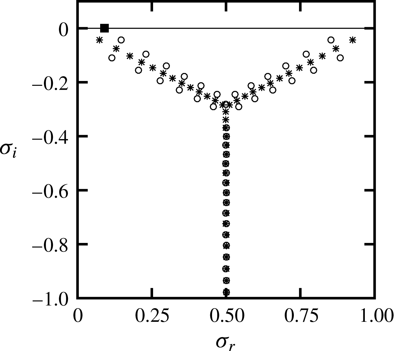
). Figure 4 shows the complete spectrum computed for the case where the same fluid occupies both layers with
 $Re=5000$
,
 $\unicode[STIX]{x1D6FC}=1$
,
 $\unicode[STIX]{x1D6FD}=0$
and
 $n=0.1$
. There is one neutrally stable mode for this case which corresponds to a solution with zero disturbance field (
 $v_{1}=v_{2}=\unicode[STIX]{x1D702}_{1}=\unicode[STIX]{x1D702}_{2}=0$
). The corresponding eigenvalue is the solution of the kinematic condition (2.9) which gives
 $\unicode[STIX]{x1D70E}=\unicode[STIX]{x1D6FC}n/(m+n)$
and
 $H=1$
. For this particular case there is no interface between the layers, and the kinematic condition is redundant. If one removes this neutrally stable mode, then the spectrum is identical to the single-layer Couette flow spectrum (Schmid & Henningson Reference Schmid and Henningson2001, p. 67), which confirms the consistency of our formulation in the limit of a single-fluid system.
Eigenvalue spectrum for
 $Re=5000$
,
 $\unicode[STIX]{x1D6FC}=1$
,
 $\unicode[STIX]{x1D6FD}=0$
,
 $m=1$
,
 $n=0.1$
,
 $r=1$
and
 $F=\unicode[STIX]{x1D6E4}=0$
. Symbols ○ and * denote OS and Sq modes, respectively; ▪ denotes the interfacial mode which is neutrally stable for this case with
 $\unicode[STIX]{x1D70E}=\unicode[STIX]{x1D6FC}n/(m+n)=0.090909$
.

Figure 5 shows the spectrum for two-fluid Couette flow where the only fluid property that is different between the two layers is the viscosity, that is,
 $m\neq 1$
. The spectra are shown for two cases with
 $m<1$
and for two cases with
 $m>1$
, all for
 $n=0.1$
. In contrast to the case with
 $m=1$
, the top eigenvalue for each case with
 $m\neq 1$
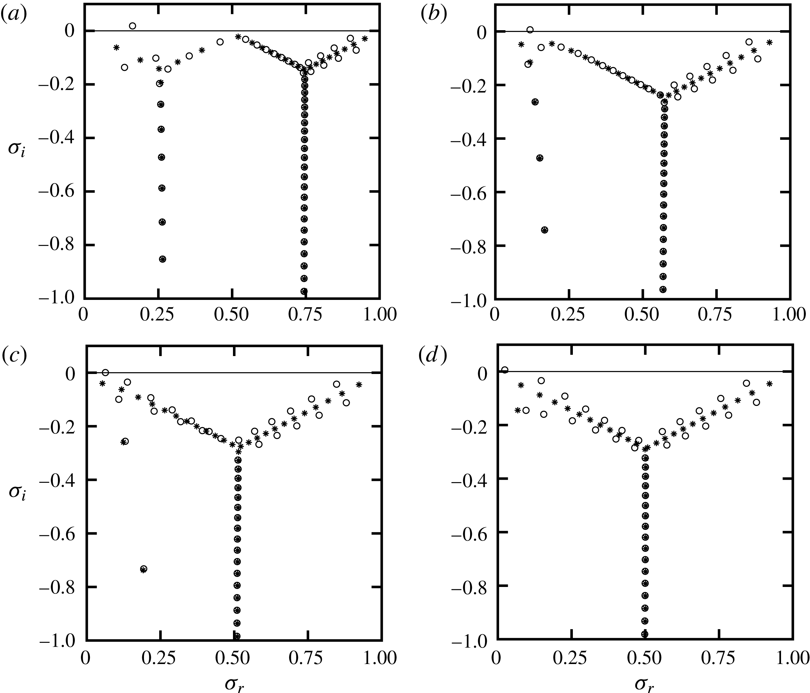
is a physical solution of the problem, commonly referred to as the interfacial mode, and it produces a non-zero disturbance field. The viscosity contrast causes the single Y-shaped spectrum to rearrange, and for some cases (depending on
 $m$
and
 $n$
) we observe two Y-shaped spectra. The base of each spectrum contains stable modes (modes that form a near-vertical line), sometimes referred to as mean modes because they travel with phase speeds that are approximately equal to the average velocity of the mean flow of that fluid layer. As
 $m$
exceeds 0.1, the average velocities of the upper and lower layers decrease from 0.75 and 0.25, and approach 0.5 and 0 at large
 $m$
, respectively (see figure 3). Figure 5 shows the same behaviour for the phase speeds of the mean modes of each fluid layer.
Eigenvalue spectra for
 $n=0.1$
: (a)
 $m=0.1$
; (b)
 $m=0.5$
; (c)
 $m=2$
; (d)
 $m=10$
. The top eigenvalue is
 $\unicode[STIX]{x1D70E}=0.163412+0.017153\text{i}$
,
 $0.118760+0.005008\text{i}$
,
 $0.064347-0.000628\text{i}$
and
 $0.024623+0.004714\text{i}$
in (a), (b), (c) and (d), respectively. Other conditions are as in figure 4.

We find that, for
 $Re=5000$
, thickness ratio
 $n=0.1$
and disturbance wavenumber of
 $\unicode[STIX]{x1D6FC}=1$
, the interfacial mode is stable when
 $1<m<2.44$
, and unstable for other values of
 $m$
. As the viscosity ratio
 $m$
increases, the left Y-shaped part of the spectrum containing modes with small phase speeds gradually disappears, and the spectrum for
 $m\gtrsim 10$
becomes very similar to the spectrum of single-fluid Couette flow (compare figures 5
d and 4). This is not unexpected because for this case we have a thin lower layer of very viscous fluid which for the upper bulk fluid appears almost as an extension of the solid wall. One of the important differences between the two spectra shown in figures 4 and 5(d) is that for
 $m=10$
we have an unstable interfacial mode with a very small phase speed, whereas for
 $m=1$
the interfacial mode is neutrally stable.
Eigenvalue spectra for
 $m=0.5$
: (a)
 $n=0.25$
; (b)
 $n=0.5$
; (c)
 $n=1$
; (d)
 $n=2$
. The top eigenvalue is
 $\unicode[STIX]{x1D70E}=0.222972+0.001265\text{i}$
,
 $0.370162+0.000025\text{i}$
,
 $0.540330-0.001096\text{i}$
and
 $0.696575-0.002493\text{i}$
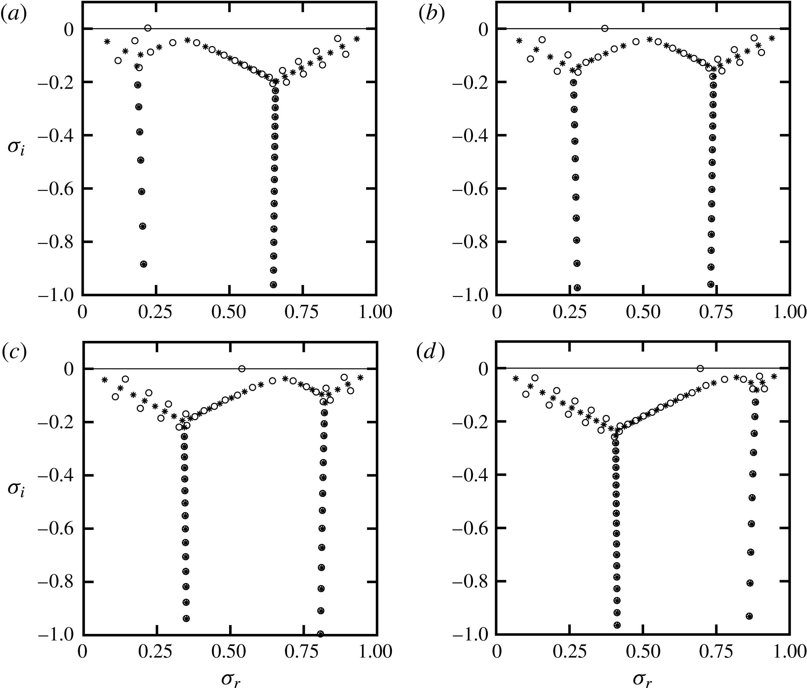
in (a), (b), (c) and (d), respectively. Other conditions are as in figure 4.

The thickness ratio
 $n$
also has a strong impact on the shape of the spectrum, as illustrated in figure 6 for
 $m=0.5$
. As discussed in § 2 and also shown in figure 3, increasing
 $n$
for a fixed
 $m$
results in a monotonic increase of both
 $U_{1,a}$
and
 $U_{2,a}$
. For instance, as
 $n$
increases from 0.1 to 2 (see figure 3),
 $U_{1,a}$
increases from approximately
 $0.6$
to approximately
 $0.9$
, while
 $U_{2,a}$
increases from approximately
 $0.1$
to approximately
 $0.4$
. We see that the phase speeds (
 $\unicode[STIX]{x1D70E}_{r}/\unicode[STIX]{x1D6FC}$
) of the mean modes of the right and left Y-shaped parts of the spectrum (figures 5 and 6) are approximately the same as
 $U_{1,a}$
and
 $U_{2,a}$
, respectively.
Eigenfunctions for the most unstable mode shown in figure 5(b): (a) real part of streamwise velocities
 $u_{1,r},u_{2,r}$
; (b) imaginary part of streamwise velocities
 $u_{1,i},u_{2,i}$
; (c) real part of normal velocities
 $v_{1,r},v_{2,r}$
; (d) imaginary part of normal velocities
 $v_{1,i},v_{2,i}$
. Eigenfunctions are normalized with
 $\max _{y_{L}\leqslant y\leqslant 0}|u_{2}(y)|$
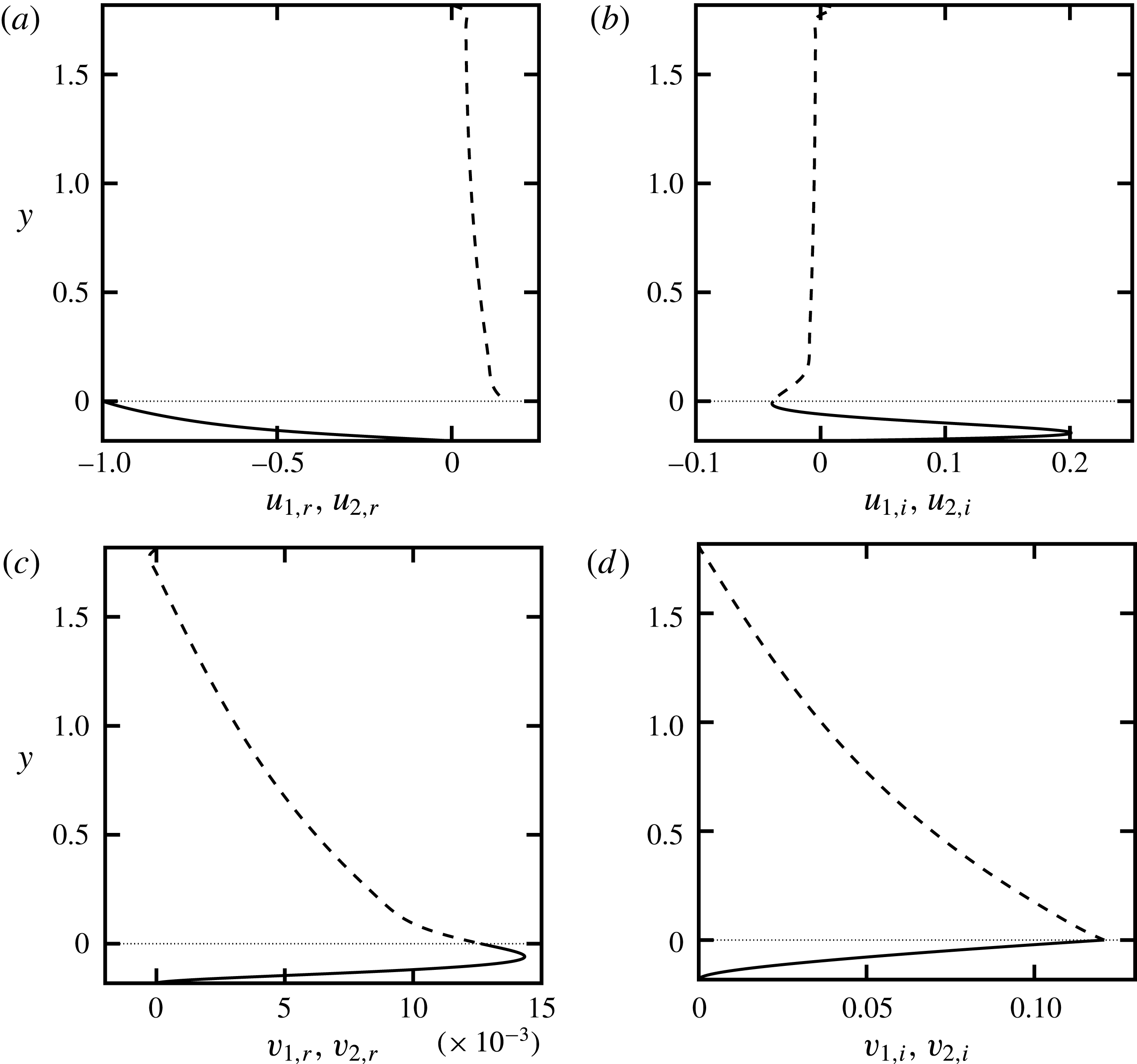
. Dashed and solid lines denote upper and lower fluid quantities, respectively, and dotted lines denote the location of the interface.

The eigenfunctions corresponding to the most unstable mode, that is, the interfacial mode of figure 5(b), are shown in figure 7 (for two-dimensional disturbances
 $w_{1}=w_{2}=0$
). When the base flows have different slopes at the interface, that is,
 $m\neq 1$
, it can be shown that the streamwise disturbance velocity (
 $u^{\prime }$
) becomes discontinuous at the interface (see appendix B), which can give rise to an unstable interfacial mode (Yih Reference Yih1967). Figure 7(a) clearly shows this discontinuity. The magnitudes of both
 $u_{2,r}$
and
 $u_{2,i}$
are much larger than
 $u_{1,r}$
and
 $u_{1,i}$
, and they are at least an order of magnitude larger than
 $v_{j,r}$
and
 $v_{j,i}$
(
 $j=1,2$
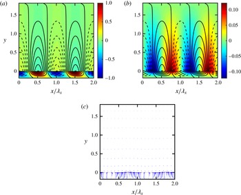
), so that the disturbance velocity field in the lower layer is nearly parallel to the wall. Figure 8(a,b) shows the disturbance streamwise and normal velocity components, respectively. The isocontours of disturbance streamfunction indicate that the flow structure consists of a set of spanwise rolls of alternating sign propagating in the streamwise direction. The streamfunction contours are much more closely packed in the lower layer, which again signals the much stronger flow in the lower layer compared to the upper layer, and figure 8(c) further reinforces this observation.
Disturbance field for the most unstable mode of figure 5(b) shown over two streamwise wavelengths,
 $2\unicode[STIX]{x1D706}_{x}$
, where
 $\unicode[STIX]{x1D706}_{x}=2\unicode[STIX]{x03C0}/\unicode[STIX]{x1D6FC}$
. (a) Colour contour: disturbance streamwise velocity components
 $u_{1}^{\prime }$
and
 $u_{2}^{\prime }$
. (b) Colour contour: disturbance normal velocity components
 $v_{1}^{\prime }$
and
 $v_{2}^{\prime }$
. Velocity components in (a) and (b) are normalized with the maximum value of
 $|u_{2}^{\prime }(x,y,0,0)|$
for
 $0\leqslant x\leqslant \unicode[STIX]{x1D706}_{x},y_{L}\leqslant y\leqslant 0$
. Isocontours in (a) and (b) denote the disturbance streamfunction placed apart by 0.02 increment (solid and dashed lines denote positive and negative values, respectively). (c) Disturbance velocity vectors at
 $z=t=0$
. Vectors are rescaled in such a way that they do not overlap. The dotted line denotes the location of the interface.

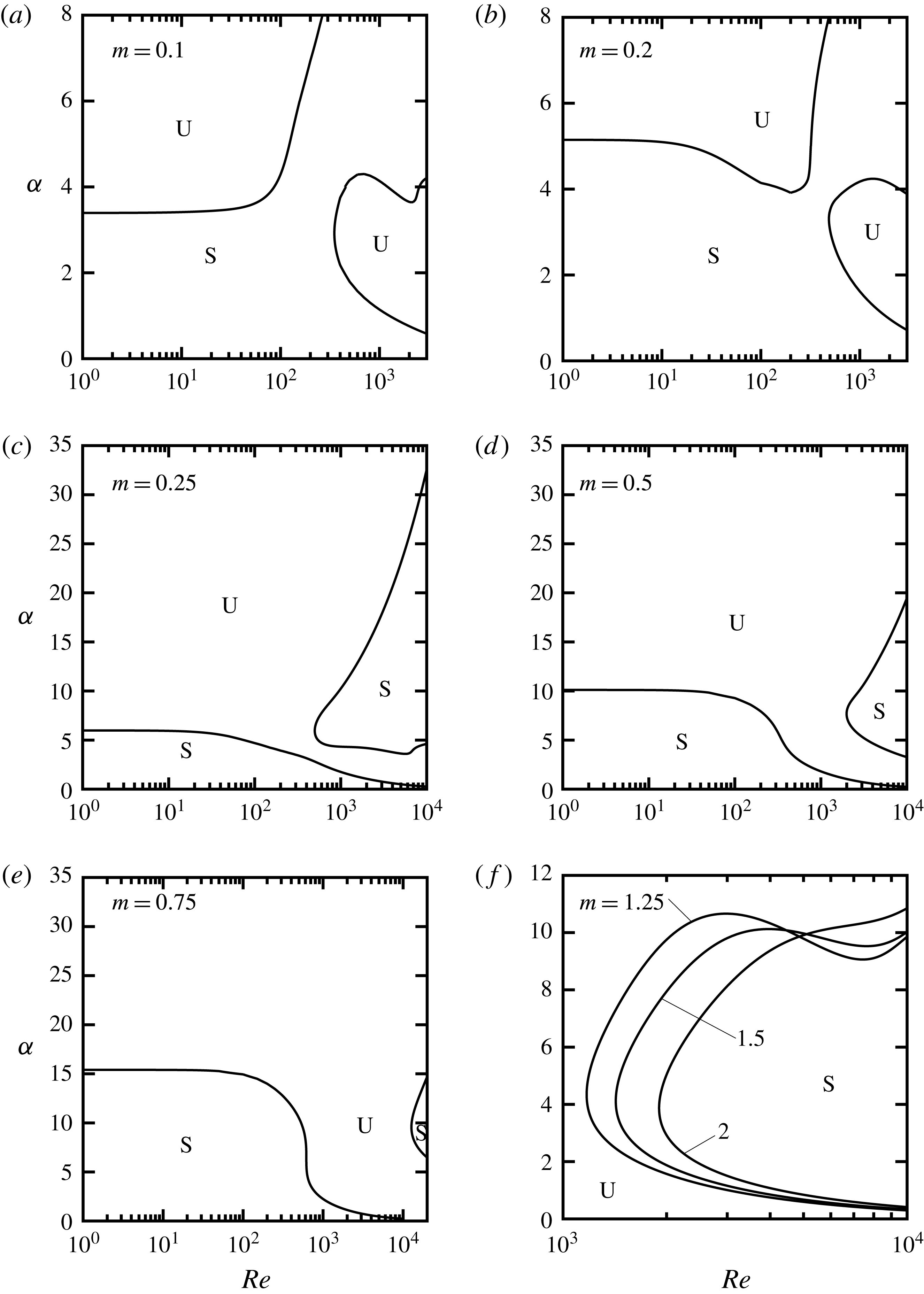
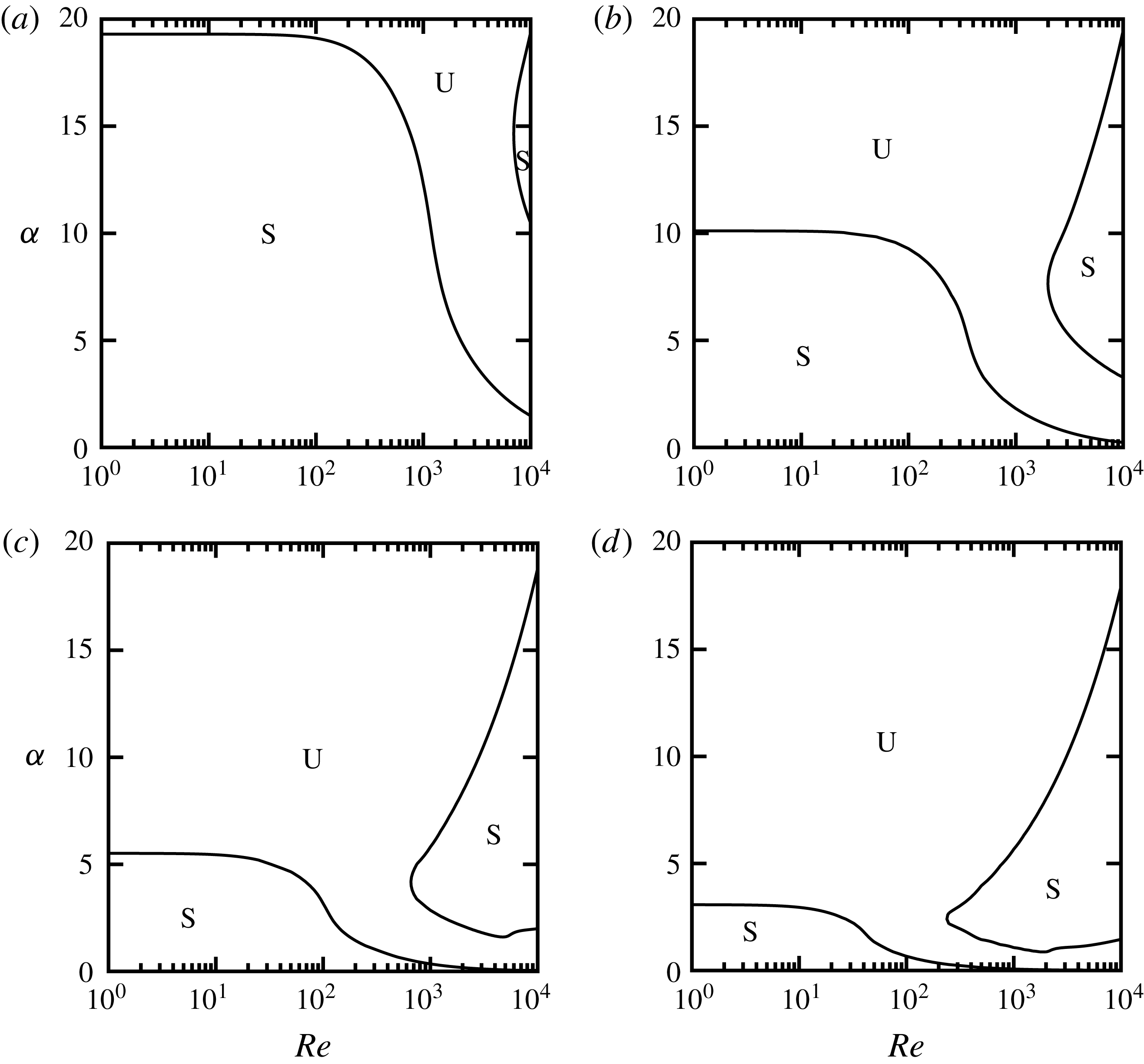
With the help of eigenvalue tracing methods such as inverse iteration or Newton–Raphson methods (Floryan Reference Floryan2002), we can produce neutral stability curves in any two-dimensional plane. Figure 9 shows neutral stability curves for the interfacial mode in the
 $(Re,\unicode[STIX]{x1D6FC})$
-plane. For viscosity ratios
 $m<1$
(see figure 9
a,b), the interfacial mode becomes unstable in two zones, one corresponding to short wavelengths (large
 $\unicode[STIX]{x1D6FC}$
) and small
 $Re$
, and one corresponding to moderate
 $\unicode[STIX]{x1D6FC}$
and large
 $Re$
. As
 $m$
increases while remaining less than one, the two unstable zones grow in size until they merge and form one large unstable zone, while the initial single stable zone (see figure 9
a,b) splits into two (see figure 9
c–e).
The neutral curves for
 $m<1$
in the limit of
 $Re$
going to zero become nearly horizontal, and the critical wavenumber
 $\unicode[STIX]{x1D6FC}_{cr}$
separating the stable and unstable zones increases with increasing
 $m$
. At
 $m=1$
, the interfacial mode becomes neutrally stable; for this particular case (where
 $r=1$
,
 $F=\unicode[STIX]{x1D6E4}=0$
), there is no interface. The shapes of the neutral curves are entirely different for
 $m>1$
(figure 9
f) compared with
 $m<1$
(figure 9
a–e). For
 $m>1$
, the stable zone is limited to moderate values of
 $\unicode[STIX]{x1D6FC}$
and large Reynolds number, and increasing
 $m$
increases the size of the unstable zone. The results shown in figure 9 agree with the long-wave (
 $\unicode[STIX]{x1D6FC}\rightarrow 0$
) solution of Yih (Reference Yih1967), who predicted that for
 $m<1$
and
 $n>1$
(or
 $m>1$
and
 $n<1$
) the interfacial mode is unstable, and that for
 $m<1$
and
 $n\lesssim 0.4$
(or
 $m>1$
and
 $n\gtrsim 2.5$
) the interfacial mode is stable in the limit of
 $\unicode[STIX]{x1D6FC}\rightarrow 0$
.
Neutral stability curves for
 $\unicode[STIX]{x1D6FD}=0$
,
 $n=0.1$
,
 $r=1$
and
 $F=\unicode[STIX]{x1D6E4}=0$
for moderate values of
 $m$
: (a)
 $m=0.1$
; (b)
 $m=0.2$
; (c)
 $m=0.25$
; (d)
 $m=0.5$
; (e)
 $m=0.75$
; (f)
 $m=1.25$
, 1.5, 2. Labels S and U denote stable and unstable zones, respectively.

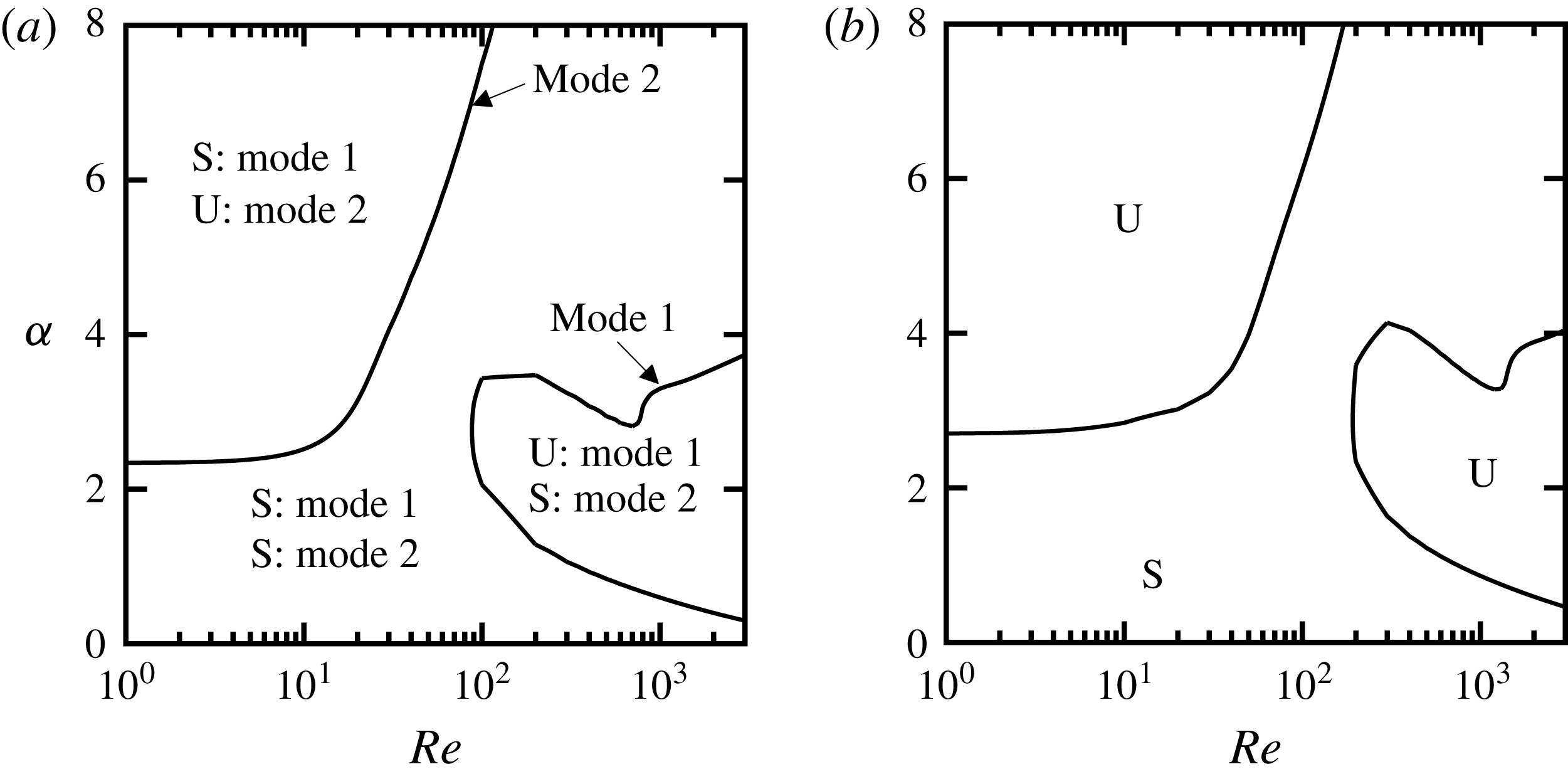
Figure 10 shows neutral curves for small viscosity ratios, specifically for
 $m=0.02$
and
 $m=0.05$
. The viscosity ratio
 $m=0.02$
corresponds to a film of air underlying a bulk flow of water, as found in drag reduction applications using SHS, although at this point we do not consider the effects of
 $r$
,
 $F$
and
 $\unicode[STIX]{x1D6E4}$
(these effects will be considered for a real water–air system later in the paper). As can be seen, the two cases are relatively similar in shape, but for
 $m<0.05$
the two unstable zones are created by two distinct modes of the spectrum. For
 $m\geqslant 0.05$
only one mode becomes unstable.
Neutral stability curves for
 $\unicode[STIX]{x1D6FD}=0$
,
 $n=0.1$
,
 $r=1$
and
 $F=\unicode[STIX]{x1D6E4}=0$
: (a)
 $m=0.02$
; (b)
 $m=0.05$
. Two distinct modes become unstable when
 $m=0.02$
; however, at
 $m=0.05$
the same interfacial mode becomes unstable in the two unstable zones. Labels S and U denote stable and unstable zones, respectively. Our results show that for
 $m<0.05$
two unstable zones are created by two separate modes, and for
 $m\geqslant 0.05$
, if two unstable zones exist, the same mode becomes unstable in those zones.

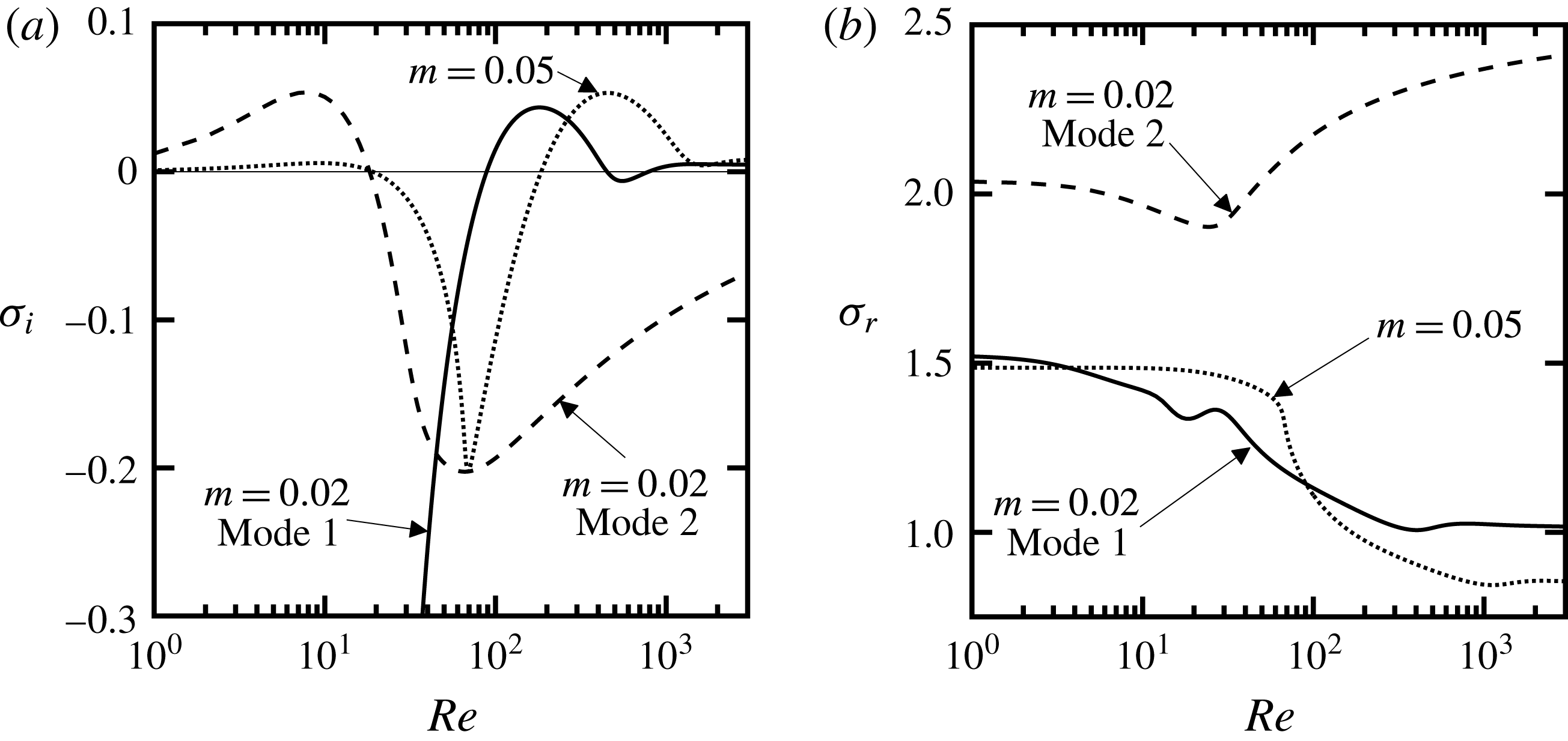
Variations of imaginary (a) and real (b) parts of the amplification rate of the most unstable modes as a function of
 $Re$
for
 $\unicode[STIX]{x1D6FC}=3$
,
 $\unicode[STIX]{x1D6FD}=0$
,
 $n=0.1$
,
 $r=1$
and
 $F=\unicode[STIX]{x1D6E4}=0$
. Solid and dashed lines denote modes 1 and 2 for
 $m=0.02$
, respectively, and dotted lines denote
 $m=0.05$
. Other conditions are as in figure 10.

To better demonstrate this phenomenon, we performed eigenvalue tracing of the top eigenvalue as a function of
 $Re$
for
 $\unicode[STIX]{x1D6FC}=3$
, chosen in such a way that it crosses both unstable zones of figure 10(a,b). This is equivalent to making horizontal cuts in figure 10(a,b) at
 $\unicode[STIX]{x1D6FC}=3$
. The results are shown in figure 11. Solid lines marked by mode 1 for
 $m=0.02$
are obtained by tracing the unstable mode from high
 $Re$
to low
 $Re$
, and dashed lines marking mode 2 for
 $m=0.02$
are obtained by tracing the unstable mode from low
 $Re$
to high
 $Re$
. These results clearly demonstrate that each unstable zone is created by a separate mode for
 $m=0.02$
. The real part of mode 2 is always greater than that of mode 1 (see figure 11
b), which indicates that mode 2 travels at faster phase speeds compared with mode 1. Performing the same test for
 $m=0.05$
, just one curve is obtained, regardless of whether we trace from high
 $Re$
to low
 $Re$
or the other way around (see dotted lines in figure 11). Additional tests confirmed that the second mode only becomes unstable at small
 $Re$
for
 $m<0.05$
and attenuates when mode 1 becomes unstable at high
 $Re$
(figure 11
a). Comparing
 $\unicode[STIX]{x1D70E}_{i}$
for
 $m=0.05$
(dotted line) with that of modes 1 and 2 reveals that at high
 $Re$
the amplification rate behaves like mode 1, but at low
 $Re$
its behaviour resembles mode 2. However,
 $\unicode[STIX]{x1D70E}_{r}$
for
 $m=0.05$
varies in the same manner as mode 1 for
 $m=0.02$
over the whole range of
 $Re$
considered here (figure 11
b).
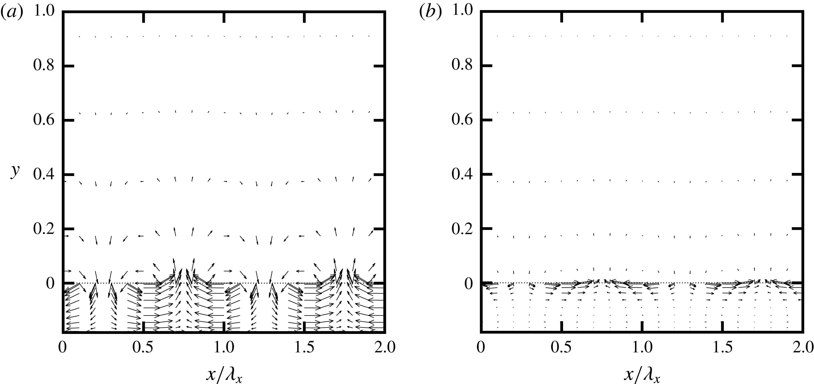
Figure 12(a,b) shows the flow topology created by modes 1 and 2, respectively, where the flow conditions were chosen based on the unstable zones of figure 10(a). For both cases, the disturbance flows are more intense in the lower layer. The disturbance field created by mode 1 extends almost across the whole thickness of the lower fluid, but for mode 2 it quickly diminishes as we move down from the interface. In the upper layer, mode 1 creates significant disturbances near the interface, but they rapidly diminish in magnitude away from the interface. In contrast, the disturbances in the upper layer created by mode 2 are very much smaller than those produced by the same mode in the lower layer.
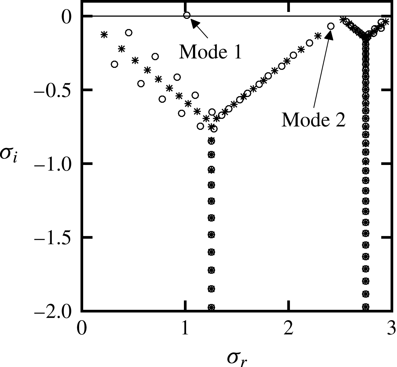
Figure 13 shows the position of modes 1 and 2 in the complete spectrum computed for
 $m=0.02$
. We see that mode 1 is the classic interfacial mode first discovered by Yih (Reference Yih1967). Mode 2 also has strong activity near the interface, but it is only active at low
 $Re$
, eliminating the possibility that it is a TS wave, and suggesting that this mode is another type of interfacial mode with properties that are different from Yih’s original interfacial mode. This appears to be a new result.
Disturbance velocity vectors at
 $z=t=0$
for the unstable mode 1 and mode 2 of figure 10(a) shown over two streamwise wavelengths,
 $2\unicode[STIX]{x1D706}_{x}$
: (a) mode 1 with
 $Re=3000$
,
 $\unicode[STIX]{x1D6FC}=3$
; (b) mode 2 with
 $Re=1$
,
 $\unicode[STIX]{x1D6FC}=3$
. Vectors are scaled in such a way that they do not overlap. Dotted line denotes the location of the interface. Other conditions are as in figure 10(a). Results are shown only in the range
 $y_{L}\leqslant y\leqslant 1$
for better legibility.


4 Similarity of the effects of thickness ratio
Two key observations can be made regarding changes in thickness ratio. First, if we interchange the layers and assume that the effects of gravity are not important, or that the fluids have equal density (that is,
 $r=1$
,
 $F=0$
), the growth rate of the disturbances in the new system is the same as that in the original system. The relations between the parameters of the flipped system and of the original system are given by
 $$\begin{eqnarray}\displaystyle & \displaystyle r^{\prime }=1/r, & \displaystyle\end{eqnarray}$$
 $$\begin{eqnarray}\displaystyle & \displaystyle m^{\prime }=1/m, & \displaystyle\end{eqnarray}$$
 $$\begin{eqnarray}\displaystyle & \displaystyle n^{\prime }=1/n, & \displaystyle\end{eqnarray}$$
 $$\begin{eqnarray}\displaystyle & \displaystyle F^{\prime }=F/r, & \displaystyle\end{eqnarray}$$
 $$\begin{eqnarray}\displaystyle & \displaystyle \unicode[STIX]{x1D6E4}^{\prime }=\unicode[STIX]{x1D6E4}/r, & \displaystyle\end{eqnarray}$$
 $$\begin{eqnarray}\displaystyle & \displaystyle Re^{\prime }=rRe/m, & \displaystyle\end{eqnarray}$$
 $$\begin{eqnarray}\displaystyle & \displaystyle \unicode[STIX]{x1D6FC}^{\prime }=\unicode[STIX]{x1D6FC}, & \displaystyle\end{eqnarray}$$
 $$\begin{eqnarray}\displaystyle & \displaystyle \unicode[STIX]{x1D6FD}^{\prime }=\unicode[STIX]{x1D6FD}, & \displaystyle\end{eqnarray}$$
 $$\begin{eqnarray}\displaystyle & \displaystyle \unicode[STIX]{x1D70E}_{r}^{\prime }=\unicode[STIX]{x1D6FC}-\unicode[STIX]{x1D70E}_{r}, & \displaystyle\end{eqnarray}$$
 $$\begin{eqnarray}\displaystyle & \displaystyle \unicode[STIX]{x1D70E}_{i}^{\prime }=\unicode[STIX]{x1D70E}_{i}, & \displaystyle\end{eqnarray}$$
 $n\leqslant 1$
and the results for
 $n>1$
can be deduced with the help of equations (4.1).
Neutral stability curves for
 $\unicode[STIX]{x1D6FD}=0$
,
 $m=0.5$
,
 $r=1$
and
 $F=\unicode[STIX]{x1D6E4}=0$
: (a)
 $n=0.05$
; (b)
 $n=0.1$
; (c)
 $n=0.2$
; (d)
 $n=0.4$
. Labels S and U denote stable and unstable zones, respectively.

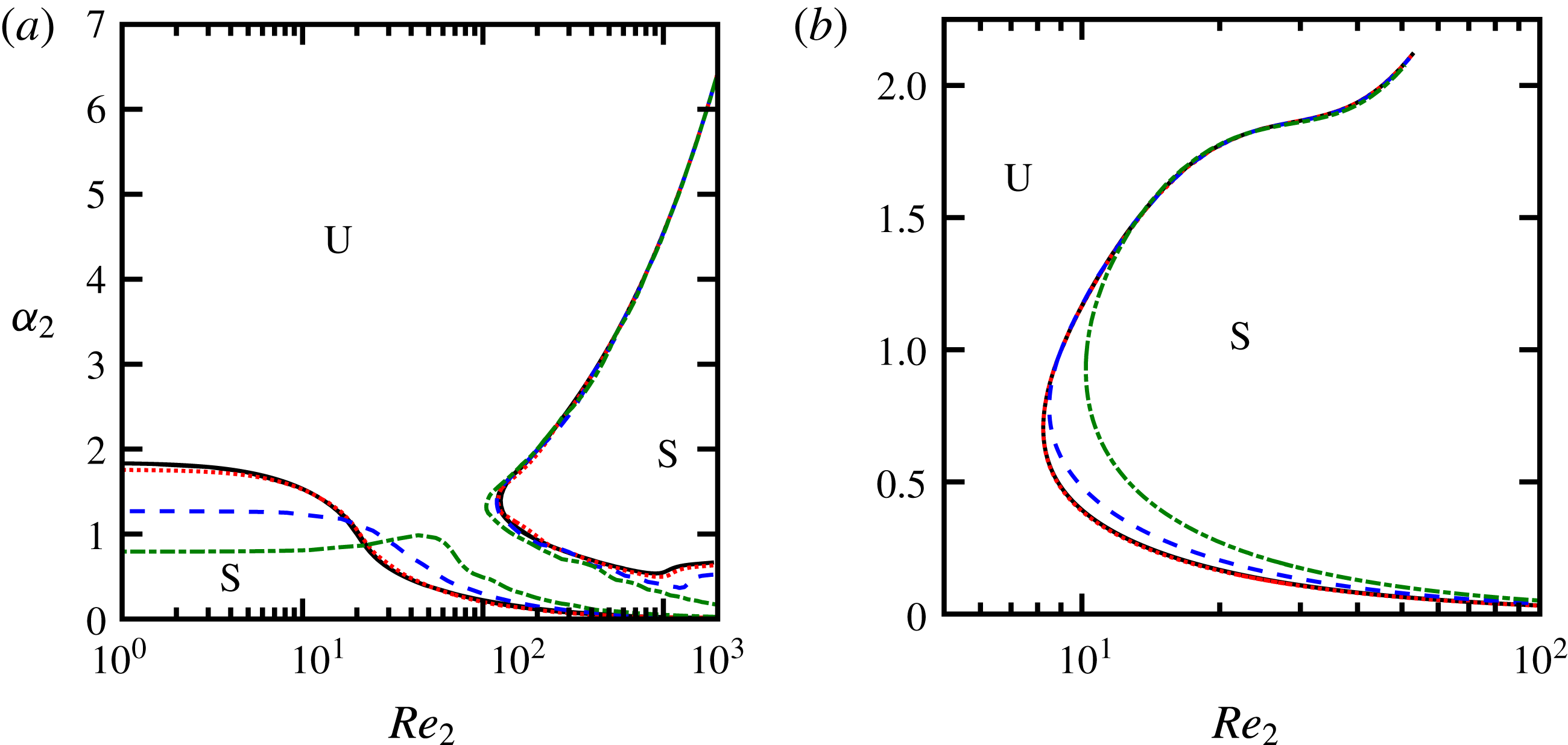
Neutral stability curves in
 $(Re_{2},\unicode[STIX]{x1D6FC}_{2})$
-plane for
 $\unicode[STIX]{x1D6FD}=0$
,
 $r=1$
and
 $F=\unicode[STIX]{x1D6E4}=0$
: (a)
 $m=0.5$
; (b)
 $m=2$
. See text and (4.2) for definitions of
 $Re_{2}$
and
 $\unicode[STIX]{x1D6FC}_{2}$
. Solid (black) lines denote
 $n=0.05$
, 0.1 and 0.2, which all are collapsed onto two curves in panel (a) and one curve in panel (b) within the resolution of these panels. Dotted (red), dashed (blue) and dashed-dotted (green) lines denote
 $n=0.4$
, 0.6 and 0.8, respectively. Labels S and U denote stable and unstable zones, respectively.

Second, we note an apparent self-similarity of the spectra for thin films. Figure 14 shows neutral curves in the
 $(Re,\unicode[STIX]{x1D6FC})$
-plane for some particular thickness ratios for
 $m=0.5$
. As
 $n$
increases,
 $\unicode[STIX]{x1D6FC}_{cr}$
decreases, and the size of the left stable zone shrinks while the unstable zone and the right stable zone expand. We see that
 $\unicode[STIX]{x1D6FC}_{cr}$
varies inversely with the thickness of the lower fluid
 $2n/(1+n)$
; as
 $n$
increases, the thickness of the less viscous fluid increases, allowing unstable waves of longer wavelengths to survive at low to moderate
 $Re$
. If we replot these results using the Reynolds number and wavenumber corresponding to the lower fluid, all curves collapse, as long as the thickness ratio
 $n\lesssim 0.4$
(figure 15). That is, the new Reynolds number
 $Re_{2}$
is defined based on the fluid properties of the lower layer (
 $\unicode[STIX]{x1D70C}_{2}$
and
 $\unicode[STIX]{x1D707}_{2}$
), the interface velocity (
 $U_{int}=n/(m+n)$
; see (2.1)) and the thickness of the lower layer (
 $d_{2}$
). The new wavenumber
 $\unicode[STIX]{x1D6FC}_{2}$
is the streamwise wavenumber non-dimensionalized with the thickness of the lower layer (
 $d_{2}$
). Specifically,
 $$\begin{eqnarray}\displaystyle & \displaystyle Re_{2}=\frac{\unicode[STIX]{x1D70C}_{2}U_{int}d_{2}}{\unicode[STIX]{x1D707}_{2}}=\left[\frac{2rn^{2}}{m(m+n)(1+n)}\right]Re, & \displaystyle\end{eqnarray}$$
 $$\begin{eqnarray}\displaystyle & \displaystyle \unicode[STIX]{x1D6FC}_{2}=\left(\frac{2n}{1+n}\right)\unicode[STIX]{x1D6FC}. & \displaystyle\end{eqnarray}$$
For
 $n>0.4$
, this self-similarity begins to fail, especially for small wavenumbers (
 $\unicode[STIX]{x1D6FC}_{2}\lesssim 1.5$
), indicating that the lower layer thickness no longer serves as a good length scale for long waves. Nevertheless, the scaling continues to work well for shorter waves (
 $\unicode[STIX]{x1D6FC}_{2}>2$
), even for thickness ratios as large as
 $n=0.8$
. The success of this scaling significantly reduces the computational cost for cases where small thickness ratios are of interest, such as in the study of LIS and SHS for drag reduction. For such problems, the neutral stability curves need to be computed for only one value of thickness ratio and then be generalized for other thickness ratios, reducing the total number of parameters by one.
No similar scaling can be found to collapse the neutral stability curves for changes in the viscosity ratio
 $m$
.
5 Results for three-dimensional waves
We now consider three-dimensional disturbances where both
 $\unicode[STIX]{x1D6FC}$
and
 $\unicode[STIX]{x1D6FD}$
are non-zero. The equations describing the stability of a three-dimensional flow can be reduced to an equivalent two-dimensional problem at a lower
 $Re$
, as long as Squire’s transformation exists for that problem (Squire Reference Squire1933). As a result, two-dimensional waves are most critical in regions of the parameter space where decreasing
 $Re$
has a stabilizing effect. However, in regions where decreasing
 $Re$
has a destabilizing effect, Squire’s theorem is no longer valid and a complete three-dimensional analysis is required. For example, Yiantsios & Higgins (Reference Yiantsios and Higgins1988) showed that for two-layer Poiseuille flow, even when Squire’s transformation exists for three-dimensional disturbances, Squire’s theorem is not valid for cases where
 $n<\sqrt{m}$
or
 $F<0$
, which correspond to cases where decreasing the Reynolds number has a destabilizing effect. Hence, no dimensional simplification can be made when considering the three-dimensional disturbance problem in two-layer systems.
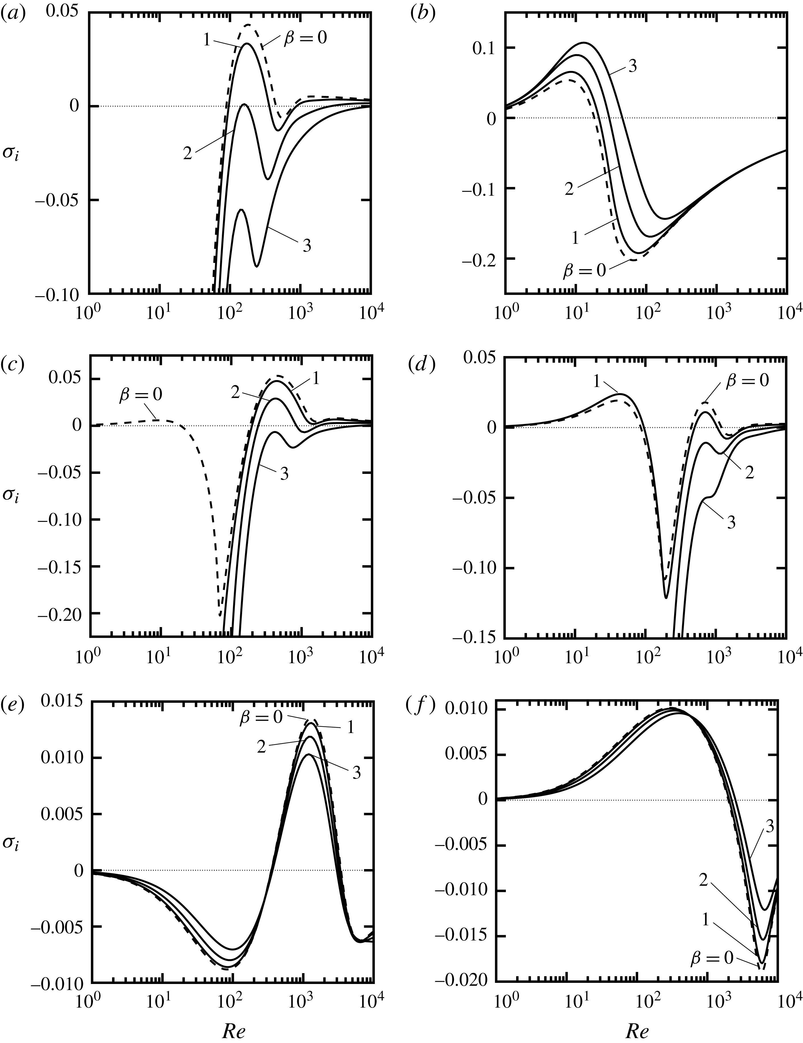
In figure 16 we show the growth rate
 $\unicode[STIX]{x1D70E}_{i}$
as a function of
 $Re$
for different spanwise disturbance wavenumbers
 $\unicode[STIX]{x1D6FD}$
. For each case, the streamwise wavenumber
 $\unicode[STIX]{x1D6FC}$
was chosen so that it crossed all stable/unstable zones of figures 9 and 10. For
 $m=0.02$
, two-dimensional waves are dominant for mode 1, whereas three-dimensional waves have higher growth rates for mode 2, as illustrated in figures 16(a) and 16(b), respectively. This result agrees with the role of
 $Re$
on stability discussed above; as seen in figure 10(a), decreasing
 $Re$
has a stabilizing effect for mode 1 and a destabilizing effect for mode 2.
At a slightly higher viscosity ratio (
 $m=0.05$
, see figure 16
c), two-dimensional waves are most critical for the whole range of
 $Re$
. For
 $m>0.05$
, the regions of dominance for either two- or three-dimensional waves are more complex (see figure 16
d–f). For instance with
 $m=0.1$
, unstable three-dimensional waves with
 $\unicode[STIX]{x1D6FD}=1$
are more critical than two-dimensional waves (
 $\unicode[STIX]{x1D6FD}=0$
) for
 $Re\lesssim 100$
, but three-dimensional waves with shorter wavelengths (
 $\unicode[STIX]{x1D6FD}=2,3$
) are highly attenuated in this Reynolds-number range. At higher
 $Re$
, three-dimensional waves are weaker than two-dimensional waves, as shown in figure 16(d). For
 $m=0.5$
, unstable two-dimensional waves dominate (figure 16
e). At even higher viscosity ratios, as shown for
 $m=2$
in figure 16(f), two-dimensional waves win over the range
 $Re\lesssim 600$
, while at higher
 $Re$
three-dimensional waves begin to dominate up to a point where all waves stabilize. This complex picture suggests that for each particular case the role of three-dimensional waves cannot be explained solely by considering the effect of Reynolds number, and all parameters need to be examined to appraise their individual effects on flow stability.
Effect of three-dimensional waves on the growth rate
 $\unicode[STIX]{x1D70E}_{i}$
for
 $n=0.1$
,
 $r=1$
and
 $F=\unicode[STIX]{x1D6E4}=0$
: (a)
 $m=0.02$
,
 $\unicode[STIX]{x1D6FC}=3$
, mode 1; (b)
 $m=0.02$
,
 $\unicode[STIX]{x1D6FC}=3$
, mode 2; (c)
 $m=0.05$
,
 $\unicode[STIX]{x1D6FC}=3$
; (d)
 $m=0.1$
,
 $\unicode[STIX]{x1D6FC}=4$
; (e)
 $m=0.5$
,
 $\unicode[STIX]{x1D6FC}=5$
; (f)
 $m=2$
,
 $\unicode[STIX]{x1D6FC}=5$
. Dashed lines denote the two-dimensional cases where
 $\unicode[STIX]{x1D6FD}=0$
.

6 Effects of interfacial tension and density ratio
Thus far, we have ignored the effects of interfacial tension and density ratio, that is, we have considered only cases where
 $r=1$
and
 $\unicode[STIX]{x1D6E4}=F=0$
. We nowbriefly analyse the effect of these parameters on the flow instability, starting with interfacial tension (
 $\unicode[STIX]{x1D6E4}\neq 0$
,
 $r=1$
and
 $F=0$
). We show the results for only one thickness ratio (
 $n=0.1$
) because the results for
 $n\lesssim 0.4$
can be determined if the scalings defined by (4.2) are used.
For
 $m=0.5$
(figure 17
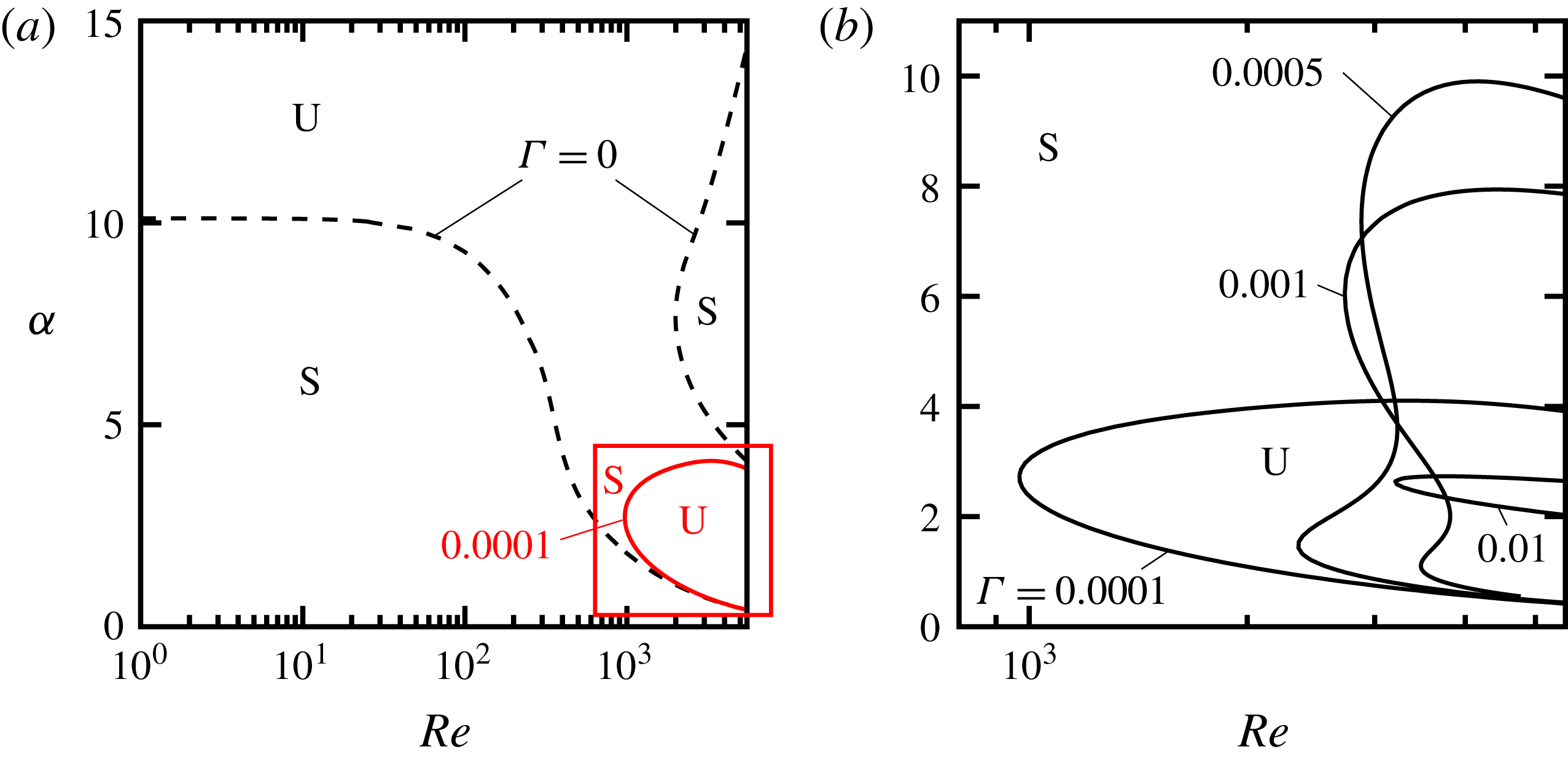
a), we see that even a very weak interfacial tension stabilizes all short waves with
 $\unicode[STIX]{x1D6FC}\gtrsim 4$
. As a result, the unstable zone is limited to long waves and high
 $Re$
, and the neutral stability curve becomes similar to the standard stability curves for TS waves. Increasing the interfacial tension leads to stronger stabilization, which manifests itself by a shift to higher
 $Re$
in the neutral curves, as shown in figure 17(b).
For
 $m=0.02$
and
 $\unicode[STIX]{x1D6E4}=0$
, two separate modes are active, as discussed in § 3 (also see figure 10
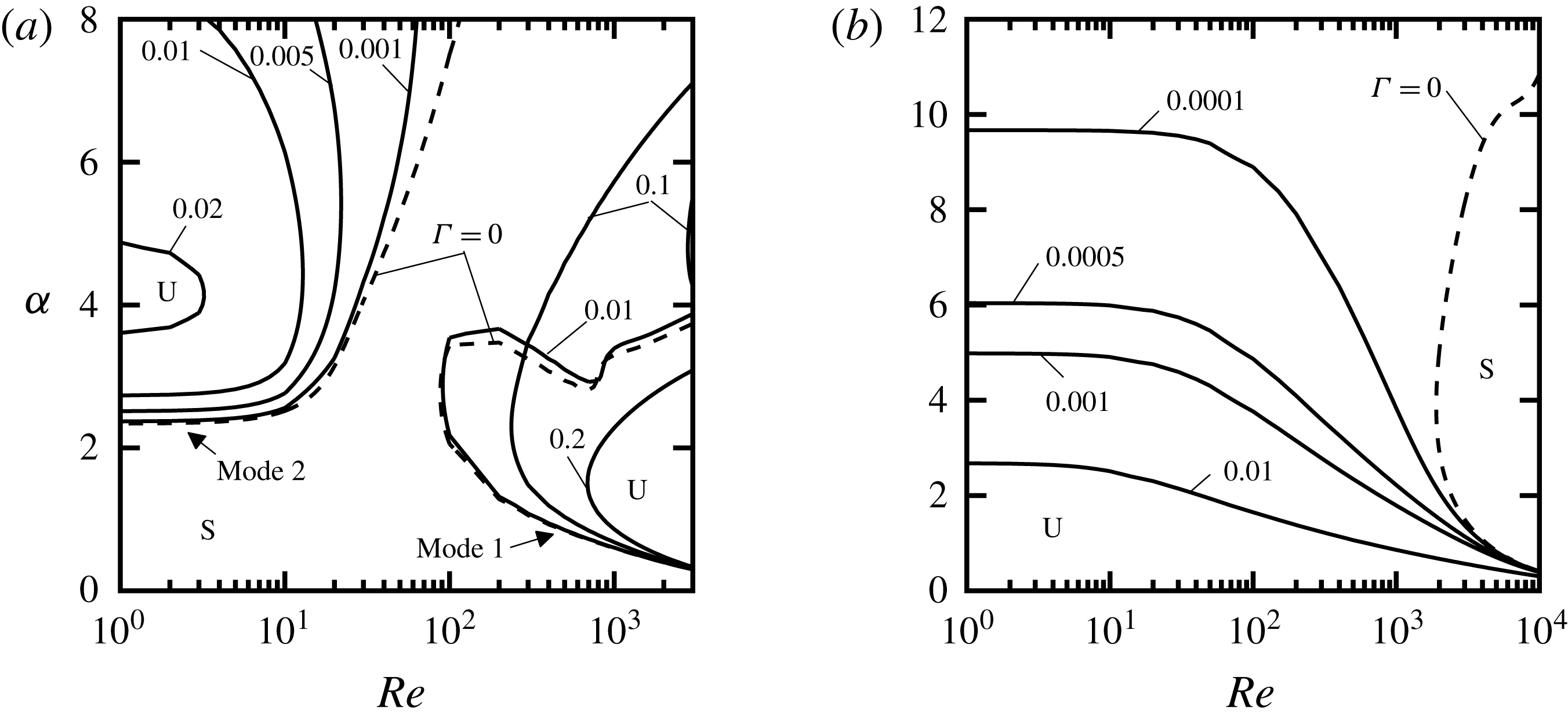
a). Figure 18(a) indicates that increasing
 $\unicode[STIX]{x1D6E4}$
decreases the size of both unstable zones. The unstable zone created by mode 2 shrinks as
 $\unicode[STIX]{x1D6E4}$
increases at a rate that is much faster than for the unstable zone generated by mode 1. For
 $m=2$
(figure 18
b), the interfacial tension stabilizes short unstable waves, and increasing
 $\unicode[STIX]{x1D6E4}$
reduces the size of the unstable zone and limits the unstable waves to waves with longer wavelengths. As a general result, interfacial tension has a significant effect on flow stability and always results in stabilization.
Neutral stability curves for varying interfacial tension, with
 $n=0.1$
,
 $r=1$
and
 $F=0$
: (a)
 $m=0.5$
; (b) enlargement of the box shown in panel (a). Dashed lines denote
 $\unicode[STIX]{x1D6E4}=0$
. Labels S and U denote stable and unstable zones, respectively.

Neutral stability curves for varying interfacial tension, with
 $n=0.1$
,
 $r=1$
and
 $F=0$
: (a)
 $m=0.02$
, results for mode 1 are shown for
 $\unicode[STIX]{x1D6E4}=0$
, 0.01, 0.1 and 0.2 while results for mode 2 are shown for
 $\unicode[STIX]{x1D6E4}=0$
, 0.001, 0.005, 0.01 and 0.02; (b)
 $m=2$
. Dashed lines denote
 $\unicode[STIX]{x1D6E4}=0$
. Labels S and U denote stable and unstable zones, respectively.

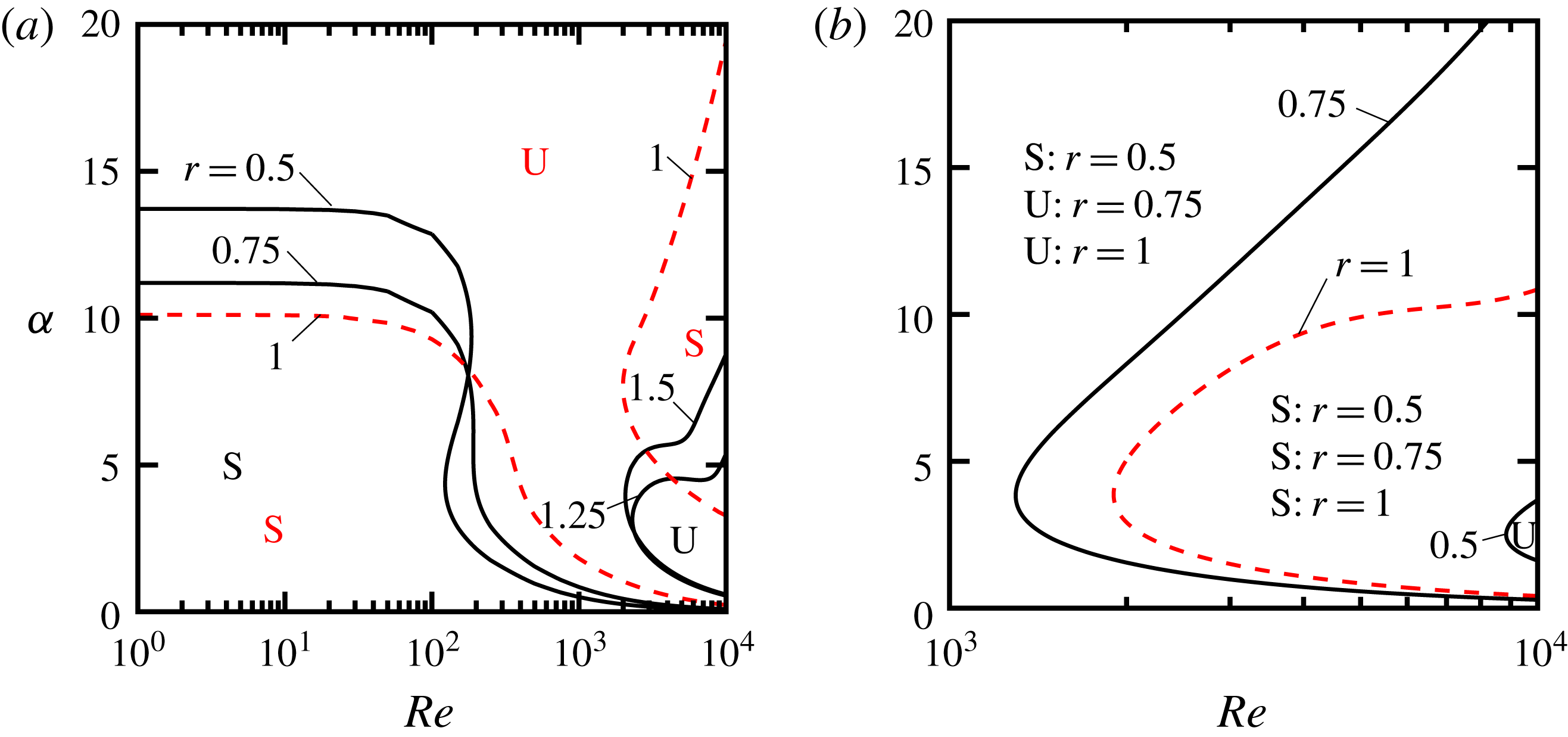
As to the effects of density ratio, figure 19 shows the effect of changing
 $r$
on the neutral curves for two viscosity ratios
 $m=0.5$
and 2 (neglecting the interfacial tension and gravity, that is,
 $\unicode[STIX]{x1D6E4}=F=0$
). The similarity scaling discussed in § 4 is still valid for these results and thus we pick only one thickness ratio,
 $n=0.1$
. For
 $m=0.5$
and
 $r=1$
, there exist two stable zones (see figure 19
a), but for
 $r<1$
only one stable zone exists and its size increases with decreasing
 $r$
. Long-wavelength disturbances are stable at low to moderate
 $Re$
while the short-wavelength disturbances are unstable at all
 $Re$
. For
 $r>1$
, the unstable zone is limited to moderate
 $\unicode[STIX]{x1D6FC}$
and high
 $Re$
, and the size of the unstable zone increases with increasing
 $r$
. For
 $m=2$
, flow is unstable for
 $r>1$
. Decreasing
 $r$
below 1 has a strong stabilization effect; the size of the stable region increases to the point where the whole region becomes stable for
 $r=0.5$
, except for a very small zone at high
 $Re$
(see figure 19
b).
Neutral stability curves for varying density ratio
 $r$
, with
 $n=0.1$
,
 $\unicode[STIX]{x1D6E4}=0$
and
 $F=0$
: (a)
 $m=0.5$
; (b)
 $m=2$
. Dashed lines denote
 $r=1$
. Labels S and U denote stable and unstable zones, respectively. Flow is unstable in the whole region of panel (b) for
 $m=2$
and
 $r=1.25$
and
 $1.5$
.

7 Results relevant to superhydrophobic surfaces and liquid-infused surfaces
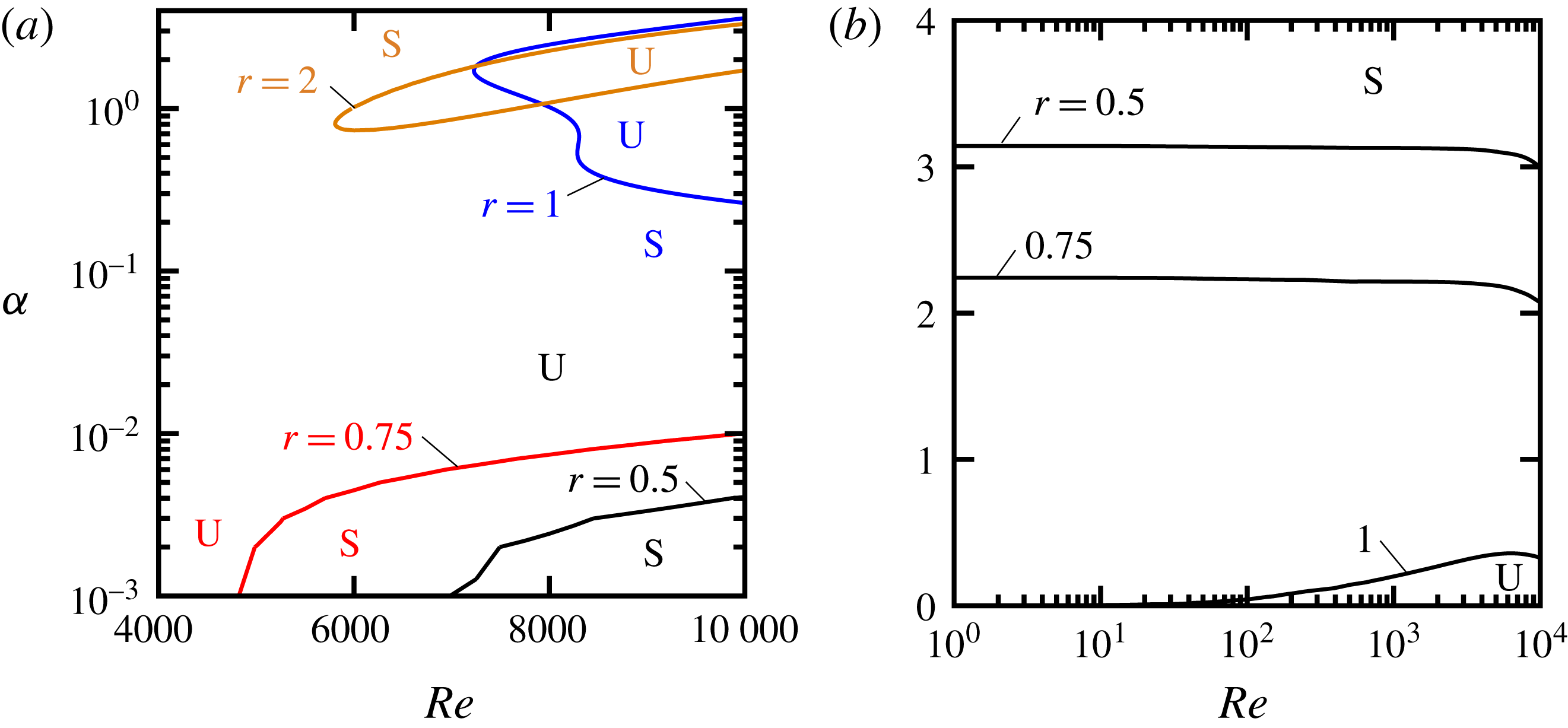
Finally, we present the neutral curves for cases that are of practical important for LIS and SHS applications. These results are computed for a channel with the half channel height of 10 mm. For LIS, we choose water as the bulk fluid (upper layer) and different alkanes as the lubricant (lower layer), as used in the experiments by Rosenberg et al. (Reference Rosenberg, Van Buren, Fu and Smits2016). For alkanes that are less viscous than water (figure 20
a) and are also less dense than water, the flow is only stable for very long waves (small
 $\unicode[STIX]{x1D6FC}$
) and moderate to high
 $Re$
. Increasing
 $r$
(for
 $r<1$
) has a stabilizing effect characterized by an increase in the size of the stable zone. For alkanes that are more dense than water (
 $r>1$
), the unstable zone is limited to
 $\unicode[STIX]{x1D6FC}$
of
 $O(1)$
and high
 $Re$
. The stability diagram changes dramatically as a function of viscosity ratio
 $m$
(compare figure 20
a and b). When the lubricant has higher viscosity than water (
 $m=2$
shown in figure 20
b), the flow stability depends largely on the disturbance wavenumber, in particular when
 $Re\lesssim 2000$
. The flow is stable for
 $\unicode[STIX]{x1D6FC}\gtrsim 3.15$
when
 $r=0.5$
and
 $Re\lesssim 2000$
. Increasing the density ratio
 $r$
has a strong stabilizing effect and, for example, the critical wavenumber separating the stable and unstable zones is reduced to
 $\unicode[STIX]{x1D6FC}_{cr}\approx 2.25$
when
 $r=0.75$
for
 $Re\lesssim 2000$
. As
 $r$
is further increased, the unstable zone becomes even smaller and is only limited to
 $\unicode[STIX]{x1D6FC}\lesssim 0.36$
and
 $Re\gtrsim 100$
. The unstable zone disappears for
 $r>1$
. For
 $r<1$
in figure 20(a) and (b) the instability is associated with the Rayleigh–Taylor instability, which is created when the gravity forces due to the density contrast are stronger than the opposing forces due to the interfacial tension (Boomkamp & Miesen Reference Boomkamp and Miesen1996).
Neutral stability curves for water as the bulk fluid (upper layer) with
 $\unicode[STIX]{x1D70C}_{1}=997~\text{kg}~\text{m}^{-3}$
and
 $\unicode[STIX]{x1D707}_{1}=0.00089~\text{kg}~(\text{m}~\text{s})^{-1}$
, and different alkanes as the lubricant (lower layer), with
 $n=0.1$
,
 $\unicode[STIX]{x1D6FE}=0.05~\text{N}~\text{m}^{-1}$
and half channel height
 $L=0.01$
m: (a)
 $m=0.5$
; (b)
 $m=2$
. Labels S and U denote stable and unstable zones, respectively. Flow is stable in the whole region of panel (b) for
 $r>1$
. Note that
 $\unicode[STIX]{x1D6E4}$
and
 $F$
vary along the curves according to
 $\unicode[STIX]{x1D6E4}=\unicode[STIX]{x1D6FE}\unicode[STIX]{x1D70C}_{1}L/(Re^{2}\unicode[STIX]{x1D707}_{1}^{2})=6.29340\times 10^{5}/Re^{2}$
and
 $F=(r-1)g\unicode[STIX]{x1D70C}_{1}^{2}L^{3}/(Re^{2}\unicode[STIX]{x1D707}_{1}^{2})=1.23106\times 10^{7}(r-1)/Re^{2}$
.

Neutral stability curves for water as the bulk fluid (upper layer) with
 $\unicode[STIX]{x1D70C}_{1}=997~\text{kg}~\text{m}^{-3}$
and
 $\unicode[STIX]{x1D707}_{1}=0.00089~\text{kg}~(\text{m}~\text{s})^{-1}$
, and air as the lower layer, with
 $m=0.0209$
,
 $n=0.1$
,
 $r=0.0012$
,
 $\unicode[STIX]{x1D6FE}=0.072~\text{N}~\text{m}^{-1}$
and half channel height
 $L=0.01~\text{m}$
. Labels S and U denote stable and unstable zones, respectively. Solid, dashed and dotted lines denote
 $n=0.1$
,
 $n=0.2$
and
 $n=0.5,1,2$
, respectively. The neutral curves corresponding to
 $n=0.5,1,2$
are very close and indistinguishable from one another within the figure resolution. Note that
 $\unicode[STIX]{x1D6E4}$
and
 $F$
vary along the curves according to
 $\unicode[STIX]{x1D6E4}=\unicode[STIX]{x1D6FE}\unicode[STIX]{x1D70C}_{1}L/(Re^{2}\unicode[STIX]{x1D707}_{1}^{2})=9.06249\times 10^{5}/Re^{2}$
and
 $F=(r-1)g\unicode[STIX]{x1D70C}_{1}^{2}L^{3}/(Re^{2}\unicode[STIX]{x1D707}_{1}^{2})=-1.22958\times 10^{7}/Re^{2}$
.

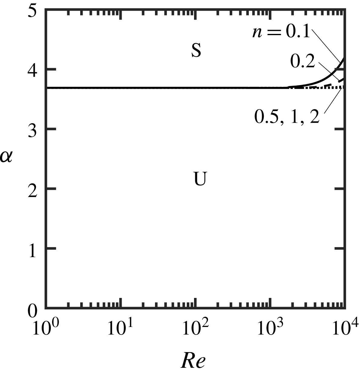
For SHS, figure 21 shows the neutral stability curves for the water–air system. There is one stable zone and one unstable zone, which persist throughout the whole range of
 $Re$
considered. The critical wavenumber separating these two zones is
 $\unicode[STIX]{x1D6FC}_{cr}\approx 3.7$
for
 $Re\lesssim 2000$
and varies in the range
 $3.7\lesssim \unicode[STIX]{x1D6FC}\lesssim 4.2$
for
 $Re\gtrsim 2000$
. The flow is unstable for wavenumbers less than the critical value, and the instabilities are again associated with the Rayleigh–Taylor instability. The neutral curves quickly lose their dependence on
 $Re$
for
 $Re\lesssim 2000$
and on
 $n$
for
 $n\gtrsim 0.5$
. The inverse Weber number
 $\unicode[STIX]{x1D6E4}$
and the gravity parameter
 $F$
vary as a function of
 $Re^{-2}$
, and at
 $Re=2000$
they are
 $\unicode[STIX]{x1D6E4}=0.23$
and
 $F=-3.07$
. The results depicted in figure 21 show that the variation of the neutral curves is already saturated at
 $Re=2000$
and further decrease of
 $Re$
(further increase of magnitudes of
 $\unicode[STIX]{x1D6E4}$
and
 $F$
) has nearly no impact on the neutral curves.
8 Conclusions
Our study of the stability of two-layer Couette flow encompassed variations in viscosity ratio, thickness ratio, density ratio and interfacial tension. It was shown that the average velocity in each layer has a strong effect on the shape of the eigenvalue spectrum by setting the phase speeds of the mean modes, and the average velocities themselves are functions of thickness and viscosity ratios. Depending on the parameters chosen, one may observe a single Y-shaped spectrum or two Y-shaped spectra. When the two fluids have different viscosities, that is,
 $m\neq 1$
, the streamwise disturbance velocity becomes discontinuous at the interface and it can give rise to an unstable interfacial mode. The disturbance velocity field created by an unstable interfacial mode shows an intense motion in the layer with lower viscosity and is characterized by normal disturbance velocities that are at least an order of magnitude smaller than the streamwise disturbance velocities.
Neutral stability diagrams were computed by eigenvalue tracings, and for low viscosity ratios, specifically
 $m=0.02$
, we found a type of interfacial mode with properties that are different from Yih’s original interfacial mode. This appears to be a new result.
When gravity is not important, the results for
 $n>1$
can be obtained from the results for
 $n<1$
by symmetry. Also, the neutral stability curves for thin films (
 $n\lesssim 0.4$
) can be collapsed onto a single curve if the Reynolds number and streamwise wavenumber are based on the properties of the lower fluid layer.
Surface tension always shrinks the unstable zones, more so for short wavelengths, and so stabilizes the flow. The effect of density ratio is more complex and cannot be easily generalized. For instance, for LIS applications with
 $m<1$
, increasing the density ratio has a stabilizing effect as long as
 $r<1$
, and a destabilizing effect for
 $r>1$
. However, for LIS with
 $m>1$
, increasing the density ratio has a stabilizing effect for all values of
 $r$
. The stability diagram for the water–air system (relevant for SHS) depends strongly on the disturbance wavenumber and the flow is stable for waves with wavenumbers greater than a critical value. The neutral curves for the water–air system lose their dependence on both
 $n$
and
 $Re$
for
 $Re\lesssim 2000$
. When the lower layer is the less dense fluid, the flow instability is governed by the Rayleigh–Taylor instabilities.
The three-dimensional stability analyses revealed that Squire’s theorem does not apply to all cases because there are regimes where increasing the Reynolds number stabilizes the flow. A full three-dimensional analysis is required.
Acknowledgements
This work was supported by the Natural Sciences and Engineering Research Council of Canada (NSERC) and the Office of Naval Research (ONR) through MURI Grant Nos. N00014-12-1-0875 and N00014-12-1-0962 (Program Manager Dr K.-H. Kim).
Appendix A. Numerical method
Standard Chebyshev polynomials defined in range
 $[-1,1]$
are used for discretization in the normal direction. The domain of each layer is mapped onto
 $[-1,1]$
using the transformation
 $$\begin{eqnarray}{\hat{y}}=\left\{\begin{array}{@{}ll@{}}E_{1}y-1,\quad & 0\leqslant y\leqslant y_{U},\\ E_{2}y-1,\quad & y_{L}\leqslant y\leqslant 0,\end{array}\right.\end{eqnarray}$$
where
 $E_{1}=1+n$
,
 $E_{2}=-(1+n)/n$
and
 ${\hat{y}}\in [-1,1]$
, the location of the interface is at
 ${\hat{y}}=-1$
and the walls are located at
 ${\hat{y}}=1$
. The basic flow, written in the
 ${\hat{y}}$
-coordinate, becomes
 $$\begin{eqnarray}\displaystyle \displaystyle U_{1}({\hat{y}}) & = & \displaystyle \hat{A}_{1}+\hat{B}_{1}{\hat{y}},\quad -1\leqslant {\hat{y}}\leqslant 1,\end{eqnarray}$$
 $$\begin{eqnarray}\displaystyle \displaystyle U_{2}({\hat{y}}) & = & \displaystyle \hat{A}_{2}+\hat{B}_{2}{\hat{y}},\quad -1\leqslant {\hat{y}}\leqslant 1,\end{eqnarray}$$
 $\hat{A}_{j}=A_{j}+(B_{j}/E_{j})$
,
 $\hat{B}_{j}=B_{j}/E_{j}$
and
 $j=1,2$
. The
 $y$
-derivatives in the new system take the form
 $$\begin{eqnarray}\text{D}^{q}=\left\{\begin{array}{@{}ll@{}}E_{1}^{q}\hat{\text{D}}^{q},\quad & \text{for the upper layer},\\ E_{2}^{q}\hat{\text{D}}^{q},\quad & \text{for the lower layer},\end{array}\right.\end{eqnarray}$$
where
 $\hat{\text{D}}^{q}=\text{d}^{q}/\text{d}{\hat{y}}^{q}$
and
 $q=1,2,3,\ldots .$
Substitution of (A 1)–(A 3) into (2.5) gives the governing equations in the computational coordinate system and takes the form
 $$\begin{eqnarray}\displaystyle & \displaystyle \left\{\frac{\text{i}}{Re}(E_{1}^{2}\hat{\text{D}}^{2}-k^{2})^{2}+\unicode[STIX]{x1D6FC}[E_{1}^{2}(U_{1}\hat{\text{D}}^{2}-\hat{\text{D}}^{2}U_{1})-k^{2}U_{1}]\right\}v_{1}=\unicode[STIX]{x1D70E}(E_{1}^{2}\hat{\text{D}}^{2}-k^{2})v_{1}, & \displaystyle \nonumber\\ \displaystyle & & \displaystyle\end{eqnarray}$$
 $$\begin{eqnarray}\displaystyle & \displaystyle (\unicode[STIX]{x1D6FD}E_{1}\hat{\text{D}}U_{1})v_{1}+\left[\frac{\text{i}}{Re}(E_{1}^{2}\hat{\text{D}}^{2}-k^{2})+\unicode[STIX]{x1D6FC}U_{1}\right]\unicode[STIX]{x1D702}_{1}=\unicode[STIX]{x1D70E}\unicode[STIX]{x1D702}_{1}, & \displaystyle\end{eqnarray}$$
 $$\begin{eqnarray}\displaystyle & \displaystyle \left\{\frac{\text{i}m}{Re}(E_{2}^{2}\hat{\text{D}}^{2}-k^{2})^{2}+r\unicode[STIX]{x1D6FC}[E_{2}^{2}(U_{2}\hat{\text{D}}^{2}-\hat{\text{D}}^{2}U_{2})-k^{2}U_{2}]\right\}v_{2}=\unicode[STIX]{x1D70E}[r(E_{2}^{2}\hat{\text{D}}^{2}-k^{2})]v_{2}, & \displaystyle \nonumber\\ \displaystyle & & \displaystyle\end{eqnarray}$$
 $$\begin{eqnarray}\displaystyle & \displaystyle (r\unicode[STIX]{x1D6FD}E_{2}\hat{\text{D}}U_{2})v_{2}+\left[\frac{\text{i}m}{Re}(E_{2}^{2}\hat{\text{D}}^{2}-k^{2})+r\unicode[STIX]{x1D6FC}U_{2}\right]\unicode[STIX]{x1D702}_{2}=\unicode[STIX]{x1D70E}r\unicode[STIX]{x1D702}_{2}. & \displaystyle\end{eqnarray}$$
The wall boundary conditions (2.7) take the form
 $$\begin{eqnarray}\displaystyle & \displaystyle v_{1}(1)=0, & \displaystyle\end{eqnarray}$$
 $$\begin{eqnarray}\displaystyle & \displaystyle \hat{\text{D}}v_{1}(1)=0, & \displaystyle\end{eqnarray}$$
 $$\begin{eqnarray}\displaystyle & \displaystyle \unicode[STIX]{x1D702}_{1}(1)=0, & \displaystyle\end{eqnarray}$$
 $$\begin{eqnarray}\displaystyle & \displaystyle v_{2}(1)=0, & \displaystyle\end{eqnarray}$$
 $$\begin{eqnarray}\displaystyle & \displaystyle \hat{\text{D}}v_{2}(1)=0, & \displaystyle\end{eqnarray}$$
 $$\begin{eqnarray}\displaystyle & \displaystyle \unicode[STIX]{x1D702}_{2}(1)=0. & \displaystyle\end{eqnarray}$$
The interfacial boundary conditions (2.8) become
 $$\begin{eqnarray}\displaystyle & \displaystyle v_{1}(-1)-v_{2}(-1)=0, & \displaystyle\end{eqnarray}$$
 $$\begin{eqnarray}\displaystyle & \displaystyle E_{1}\hat{\text{D}}v_{1}(-1)-E_{2}\hat{\text{D}}v_{2}(-1)-\text{i}\unicode[STIX]{x1D6FC}[E_{1}\hat{\text{D}}U_{1}(-1)-E_{2}\hat{\text{D}}U_{2}(-1)]H=0, & \displaystyle\end{eqnarray}$$
 $$\begin{eqnarray}\displaystyle & \displaystyle \unicode[STIX]{x1D702}_{1}(-1)-\unicode[STIX]{x1D702}_{2}(-1)+\text{i}\unicode[STIX]{x1D6FD}[E_{1}\hat{\text{D}}U_{1}(-1)-E_{2}\hat{\text{D}}U_{2}(-1)]H=0, & \displaystyle\end{eqnarray}$$
 $$\begin{eqnarray}\displaystyle & \displaystyle (E_{1}^{2}\hat{\text{D}}^{2}+k^{2})v_{1}(-1)-m(E_{2}^{2}\hat{\text{D}}^{2}+k^{2})v_{2}(-1)=0, & \displaystyle\end{eqnarray}$$
 $$\begin{eqnarray}\displaystyle & \displaystyle E_{1}\hat{\text{D}}\unicode[STIX]{x1D702}_{1}(-1)-mE_{2}\hat{\text{D}}\unicode[STIX]{x1D702}_{2}(-1)=0, & \displaystyle\end{eqnarray}$$
 $$\begin{eqnarray}\displaystyle & & \displaystyle \{E_{1}^{3}\hat{\text{D}}^{3}-3k^{2}E_{1}\hat{\text{D}}+\text{i}\unicode[STIX]{x1D6FC}Re(r-1)[U_{1}(-1)E_{1}\hat{\text{D}}-E_{1}\hat{\text{D}}U_{1}(-1)]\}v_{1}(-1)\nonumber\\ \displaystyle & & \displaystyle \qquad \quad -\,m(E_{2}^{3}\hat{\text{D}}^{3}-3k^{2}E_{2}\hat{\text{D}})v_{2}(-1)+k^{2}Re(F+k^{2}\unicode[STIX]{x1D6E4})H=\unicode[STIX]{x1D70E}[\text{i}Re(r-1)E_{1}\hat{\text{D}}]v_{1}(-1).\nonumber\\ \displaystyle & & \displaystyle\end{eqnarray}$$
The kinematic condition (2.9) in the new system takes the form
 $$\begin{eqnarray}\text{i}v_{1}(-1)+[\unicode[STIX]{x1D6FC}U_{1}(-1)]H=\unicode[STIX]{x1D70E}H.\end{eqnarray}$$
We express the unknowns as Chebyshev expansions, i.e.
 $$\begin{eqnarray}\displaystyle & \displaystyle v_{1}({\hat{y}})=\mathop{\sum }_{k=0}^{\infty }G_{v_{1},k}\,T_{k}({\hat{y}})\approx \mathop{\sum }_{k=0}^{K_{1}}G_{v_{1},k}\,T_{k}({\hat{y}}), & \displaystyle\end{eqnarray}$$
 $$\begin{eqnarray}\displaystyle & \displaystyle \unicode[STIX]{x1D702}_{1}({\hat{y}})=\mathop{\sum }_{k=0}^{\infty }G_{\unicode[STIX]{x1D702}_{1},k}\,T_{k}({\hat{y}})\approx \mathop{\sum }_{k=0}^{K_{1}}G_{\unicode[STIX]{x1D702}_{1},k}\,T_{k}({\hat{y}}), & \displaystyle\end{eqnarray}$$
 $$\begin{eqnarray}\displaystyle & \displaystyle v_{2}({\hat{y}})=\mathop{\sum }_{k=0}^{\infty }G_{v_{2},k}\,T_{k}({\hat{y}})\approx \mathop{\sum }_{k=0}^{K_{2}}G_{v_{2},k}\,T_{k}({\hat{y}}), & \displaystyle\end{eqnarray}$$
 $$\begin{eqnarray}\displaystyle & \displaystyle \unicode[STIX]{x1D702}_{2}({\hat{y}})=\mathop{\sum }_{k=0}^{\infty }G_{\unicode[STIX]{x1D702}_{2},k}\,T_{k}({\hat{y}})\approx \mathop{\sum }_{k=0}^{K_{2}}G_{\unicode[STIX]{x1D702}_{2},k}\,T_{k}({\hat{y}}), & \displaystyle\end{eqnarray}$$
 $T_{k}$
denotes the Chebyshev polynomial of the first kind of the
 $k$
th order (see Mason & Handscomb Reference Mason and Handscomb2002), and
 $G_{v_{j},k}$
and
 $G_{\unicode[STIX]{x1D702}_{j},k}$
(
 $j=1,\,2$
) are the Chebyshev coefficients. The expansions are truncated to orders
 $K_{1}$
and
 $K_{2}$
for the upper and lower fluid quantities, respectively. Substituting (A 8) into (A 4) and applying a Galerkin projection (Canuto et al.
Reference Canuto, Hussaini, Quarteroni and Zang2006) gives
 $$\begin{eqnarray}\displaystyle & & \displaystyle \mathop{\sum }_{k=0}^{K_{1}}\left\{\frac{\text{i}}{Re}(E_{1}^{4}\langle T_{j},\hat{\text{D}}^{4}T_{k}\rangle -2k^{2}E_{1}^{2}\langle T_{j},\hat{\text{D}}^{2}T_{k}\rangle +k^{4}\langle T_{j},T_{k}\rangle )\right.\nonumber\\ \displaystyle & & \displaystyle \qquad \quad \left.+\,\unicode[STIX]{x1D6FC}[E_{1}^{2}(\langle T_{j},U_{1}\hat{\text{D}}^{2}T_{k}\rangle -\langle T_{j},\hat{\text{D}}^{2}U_{1}T_{k}\rangle )-k^{2}\langle T_{j},U_{1}T_{k}\rangle ]\right\}G_{v_{1},k}\nonumber\\ \displaystyle & & \displaystyle \qquad =\unicode[STIX]{x1D70E}\mathop{\sum }_{k=0}^{K_{1}}(E_{1}^{2}\langle T_{j},\hat{\text{D}}^{2}T_{k}\rangle -k^{2}\langle T_{j},T_{k}\rangle )G_{v_{1},k},\end{eqnarray}$$
 $$\begin{eqnarray}\displaystyle & & \displaystyle \mathop{\sum }_{k=0}^{K_{1}}\left\{\unicode[STIX]{x1D6FD}E_{1}\langle T_{j},\hat{\text{D}}U_{1}T_{k}\rangle G_{v_{1},k}+\left[\frac{\text{i}}{Re}(E_{1}^{2}\langle T_{j},\hat{\text{D}}^{2}T_{k}\rangle -k^{2}\langle T_{j},T_{k}\rangle )+\unicode[STIX]{x1D6FC}\langle T_{j},U_{1}T_{k}\rangle \right]G_{\unicode[STIX]{x1D702}_{1},k}\right\}\nonumber\\ \displaystyle & & \displaystyle \qquad =\unicode[STIX]{x1D70E}\mathop{\sum }_{k=0}^{K_{1}}\langle T_{j},T_{k}\rangle G_{\unicode[STIX]{x1D702}_{1},k},\end{eqnarray}$$
 $$\begin{eqnarray}\displaystyle & & \displaystyle \mathop{\sum }_{k=0}^{K_{2}}\left\{\frac{\text{i}m}{Re}(E_{2}^{4}\langle T_{j},\hat{\text{D}}^{4}T_{k}\rangle -2k^{2}E_{2}^{2}\langle T_{j},\hat{\text{D}}^{2}T_{k}\rangle +k^{4}\langle T_{j},T_{k}\rangle )\right.\nonumber\\ \displaystyle & & \displaystyle \qquad \quad \left.+\,r\unicode[STIX]{x1D6FC}[E_{2}^{2}(\langle T_{j},U_{2}\hat{\text{D}}^{2}T_{k}\rangle -\langle T_{j},\hat{\text{D}}^{2}U_{2}T_{k}\rangle )-k^{2}\langle T_{j},U_{2}T_{k}\rangle ]\right\}G_{v_{2},k}\nonumber\\ \displaystyle & & \displaystyle \qquad =\unicode[STIX]{x1D70E}\mathop{\sum }_{k=0}^{K_{2}}r(E_{2}^{2}\langle T_{j},\hat{\text{D}}^{2}T_{k}\rangle -k^{2}\langle T_{j},T_{k}\rangle )G_{v_{2},k},\end{eqnarray}$$
 $$\begin{eqnarray}\displaystyle & & \displaystyle \mathop{\sum }_{k=0}^{K_{2}}\left\{r\unicode[STIX]{x1D6FD}E_{2}\langle T_{j},\hat{\text{D}}U_{2}T_{k}\rangle G_{v_{2},k}+\left[\frac{\text{i}m}{Re}(E_{2}^{2}\langle T_{j},\hat{\text{D}}^{2}T_{k}\rangle -k^{2}\langle T_{j},T_{k}\rangle )\right.\right.\nonumber\\ \displaystyle & & \displaystyle \qquad \quad \left.\left.+\,r\unicode[STIX]{x1D6FC}\langle T_{j},U_{2}T_{k}\rangle \right]G_{\unicode[STIX]{x1D702}_{2},k}\right\}=\unicode[STIX]{x1D70E}\mathop{\sum }_{k=0}^{K_{2}}r\langle T_{j},T_{k}\rangle G_{\unicode[STIX]{x1D702}_{2},k},\end{eqnarray}$$
 $j=0,1,2,\ldots ,K_{1}-4$
in (A 9a
),
 $j=0,1,2,\ldots ,K_{1}-2$
in (A 9b
),
 $j=0,1,2,\ldots ,K_{2}-4$
in (A 9c
) and
 $j=0,1,2,\ldots ,K_{2}-2$
in (A 9d
). The reason for removing 12 projection equations is to create space for the imposition of the 12 boundary conditions (A 5)–(A 6) (tau method; Canuto et al.
Reference Canuto, Hussaini, Quarteroni and Zang2006). In the above,
 $\langle \cdot \rangle$
denotes the inner product, which for two arbitrary functions
 $f$
and
 $g$
is defined by
 $$\begin{eqnarray}\langle f({\hat{y}}),g({\hat{y}})\rangle _{\unicode[STIX]{x1D714}}=\int _{-1}^{1}f({\hat{y}})g({\hat{y}})\unicode[STIX]{x1D714}({\hat{y}})\,\text{d}{\hat{y}},\end{eqnarray}$$
where
 $\unicode[STIX]{x1D714}({\hat{y}})=1/\sqrt{1-{\hat{y}}^{2}}$
is the weighting function. The method of evaluating different inner products can be found in Mohammadi (Reference Mohammadi2013, pp. 221–226). The discretized forms of the boundary conditions (A 5) become
 $$\begin{eqnarray}\displaystyle & \displaystyle \mathop{\sum }_{k=0}^{K_{1}}T_{k}(1)G_{v_{1},k}=0, & \displaystyle\end{eqnarray}$$
 $$\begin{eqnarray}\displaystyle & \displaystyle \mathop{\sum }_{k=0}^{K_{1}}\hat{\text{D}}T_{k}(1)G_{v_{1},k}=0, & \displaystyle\end{eqnarray}$$
 $$\begin{eqnarray}\displaystyle & \displaystyle \mathop{\sum }_{k=0}^{K_{1}}T_{k}(1)G_{\unicode[STIX]{x1D702}_{1},k}=0, & \displaystyle\end{eqnarray}$$
 $$\begin{eqnarray}\displaystyle & \displaystyle \mathop{\sum }_{k=0}^{K_{2}}T_{k}(1)G_{v_{2},k}=0, & \displaystyle\end{eqnarray}$$
 $$\begin{eqnarray}\displaystyle & \displaystyle \mathop{\sum }_{k=0}^{K_{2}}\hat{\text{D}}T_{k}(1)G_{v_{2},k}=0, & \displaystyle\end{eqnarray}$$
 $$\begin{eqnarray}\displaystyle & \displaystyle \mathop{\sum }_{k=0}^{K_{2}}T_{k}(1)G_{\unicode[STIX]{x1D702}_{2},k}=0. & \displaystyle\end{eqnarray}$$
Similarly, the discretized interfacial boundary conditions (A 6) take the form
 $$\begin{eqnarray}\displaystyle \mathop{\sum }_{k=0}^{K_{1}}T_{k}(-1)G_{v_{1},k}-\mathop{\sum }_{k=0}^{K_{2}}T_{k}(-1)G_{v_{2},k}=0, & & \displaystyle\end{eqnarray}$$
 $$\begin{eqnarray}\displaystyle & \displaystyle \mathop{\sum }_{k=0}^{K_{1}}E_{1}\hat{\text{D}}T_{k}(-1)G_{v_{1},k}-\mathop{\sum }_{k=0}^{K_{2}}E_{2}\hat{\text{D}}T_{k}(-1)G_{v_{2},k}-\text{i}\unicode[STIX]{x1D6FC}[E_{1}\hat{\text{D}}U_{1}(-1)-E_{2}\hat{\text{D}}U_{2}(-1)]H=0, & \displaystyle \nonumber\\ \displaystyle & & \displaystyle\end{eqnarray}$$
 $$\begin{eqnarray}\displaystyle & \displaystyle \mathop{\sum }_{k=0}^{K_{1}}T_{k}(-1)G_{\unicode[STIX]{x1D702}_{1},k}-\mathop{\sum }_{k=0}^{K_{2}}T_{k}(-1)G_{\unicode[STIX]{x1D702}_{2},k}+\text{i}\unicode[STIX]{x1D6FD}[E_{1}\hat{\text{D}}U_{1}(-1)-E_{2}\hat{\text{D}}U_{2}(-1)]H=0, & \displaystyle \nonumber\\ \displaystyle & & \displaystyle\end{eqnarray}$$
 $$\begin{eqnarray}\displaystyle & \displaystyle \mathop{\sum }_{k=0}^{K_{1}}(E_{1}^{2}\hat{\text{D}}^{2}+k^{2})T_{k}(-1)G_{v_{1},k}-\mathop{\sum }_{k=0}^{K_{2}}m(E_{2}^{2}\hat{\text{D}}^{2}+k^{2})T_{k}(-1)G_{v_{2},k}=0, & \displaystyle\end{eqnarray}$$
 $$\begin{eqnarray}\displaystyle & \displaystyle \mathop{\sum }_{k=0}^{K_{1}}E_{1}\hat{\text{D}}T_{k}(-1)G_{\unicode[STIX]{x1D702}_{1},k}-\mathop{\sum }_{k=0}^{K_{2}}mE_{2}\hat{\text{D}}T_{k}(-1)G_{\unicode[STIX]{x1D702}_{2},k}=0, & \displaystyle\end{eqnarray}$$
 $$\begin{eqnarray}\displaystyle & & \displaystyle \mathop{\sum }_{k=0}^{K_{1}}\{E_{1}^{3}\hat{\text{D}}^{3}-3k^{2}E_{1}\hat{\text{D}}+\text{i}\unicode[STIX]{x1D6FC}Re(r-1)[U_{1}(-1)E_{1}\hat{\text{D}}-E_{1}\hat{\text{D}}U_{1}(-1)]\}T_{k}(-1)G_{v_{1},k}\nonumber\\ \displaystyle & & \displaystyle \qquad \quad -\,\mathop{\sum }_{k=0}^{K_{2}}m(E_{2}^{3}\hat{\text{D}}^{3}-3k^{2}E_{2}\hat{\text{D}})T_{k}(-1)G_{v_{2},k}\nonumber\\ \displaystyle & & \displaystyle \qquad \quad +\,k^{2}Re(F+k^{2}\unicode[STIX]{x1D6E4})H=\unicode[STIX]{x1D70E}\mathop{\sum }_{k=0}^{K_{1}}[\text{i}Re(r-1)E_{1}\hat{\text{D}}T_{k}(-1)]G_{v_{1},k}.\end{eqnarray}$$
Finally, the discretized kinematic condition (A 7) becomes
 $$\begin{eqnarray}\mathop{\sum }_{k=0}^{K_{1}}\text{i}T_{k}(-1)G_{v_{1},k}+[\unicode[STIX]{x1D6FC}U_{1}(-1)]H=\unicode[STIX]{x1D70E}H.\end{eqnarray}$$
The above formulation is general and can be used to study linear stability of any canonical plane-parallel two-fluid system as long as the proper base flow is used. The accuracy of this formulation was verified by comparing the results with asymptotic solutions from the literature for both Couette flow (Yih Reference Yih1967) and Poiseuille flow (Yih Reference Yih1967; Yiantsios & Higgins Reference Yiantsios and Higgins1988; Kaffel & Riaz Reference Kaffel and Riaz2015). Table 1 shows an example from these tests comparing the asymptotic solution of Yih (Reference Yih1967) obtained in the limit of long-wavelength disturbances and the current numerical solution. Most of results presented in this paper have been computed using
 $K_{1}=K_{2}=100$
, which was sufficient to provide at least six digits of accuracy for the eigenvalues.
Asymptotic and numerical values of the complex wave speed
 $c$
for
 $Re=1$
,
 $\unicode[STIX]{x1D6FD}=0$
,
 $r=1$
,
 $F=0$
and
 $\unicode[STIX]{x1D6E4}=0$
.

Appendix B
In this appendix we show why the streamwise disturbance velocity is discontinuous at the interface. The total streamwise velocity is continuous at the interface, i.e.
 $$\begin{eqnarray}u_{1}(h)=u_{2}(h),\end{eqnarray}$$
where
 $h$
is the perturbed interface defined by (2.10). The total velocity can be written as a sum of the base flow plus disturbances, that is,
 $$\begin{eqnarray}U_{1}(h)+u_{1}^{\prime }(h)=U_{2}(h)+u_{2}^{\prime }(h).\end{eqnarray}$$
Using a Taylor expansion around
 $y=0$
in (B 2) gives
 $$\begin{eqnarray}\displaystyle & & \displaystyle U_{1}(0)+\frac{\text{d}U_{1}(0)}{\text{d}y}h+u_{1}^{\prime }(0)+\frac{\unicode[STIX]{x2202}u_{1}^{\prime }(0)}{\unicode[STIX]{x2202}y}h+O(h^{2})\nonumber\\ \displaystyle & & \displaystyle \qquad =U_{2}(0)+\frac{\text{d}U_{2}(0)}{\text{d}y}h+\,u_{2}^{\prime }(0)+\frac{\unicode[STIX]{x2202}u_{2}^{\prime }(0)}{\unicode[STIX]{x2202}y}h+O(h^{2}).\end{eqnarray}$$
If we ignore the nonlinear terms
 $(\unicode[STIX]{x2202}u_{j}^{\prime }(0)/\unicode[STIX]{x2202}y)h$
, where
 $j=1,\,2$
, and take into account that the base flow is continuous at the interface (
 $U_{1}(0)=U_{2}(0)$
; see (2.1)), we obtain
 $$\begin{eqnarray}\frac{\text{d}U_{1}(0)}{\text{d}y}h+u_{1}^{\prime }(0)=\frac{\text{d}U_{2}(0)}{\text{d}y}h+u_{2}^{\prime }(0).\end{eqnarray}$$
Equation (B 4) clearly shows that the streamwise disturbance velocity is discontinuous at the interface when the slope of the base flow is discontinuous, that is, when
 $m\neq 1$
. By following a similar procedure, we can show that the normal and spanwise components of the disturbance velocity are continuous at the interface.