1 Introduction
In the last century, Hakim developed a manifestly covariant statistical mechanics (Hakim I Reference Hakim1967; Hakim II Reference Hakim1967). A rigorous hierarchy of equations for suitable reduced densities is described by studying the electromagnetic interactions. In order to calculate the dispersion relations for a plasma, Prentice (Reference Prentice1968) presented an interesting work obtaining transverse and longitudinal modes including the relativistic Landau damping but without including the radiation reaction force and the internal magnetic field produced by the relativistic electrons. Later, by including the radiation reaction force calculated by Dirac (Reference Dirac1938) and all the interactions between the electrons of the plasma (retarded electric and magnetic fields), Hakim & Mangeney (Reference Hakim and Mangeney1968) obtained a relativistic Vlasov equation which permits us to obtain wave dispersion relations, the conductivity tensor and other properties. However, the use of the Lorentz–Dirac equation obligates us to consider the hyper-acceleration as an independent variable since it plays the same role as the position and the velocity. The phase space results in a
 $10N$
-dimensional space, where
 $N$
is the number of particles (
 $12N-2N$
, due to the kinematic relations). In an approximation process, by using the Lorentz–Dirac equation at first order in the characteristic time of the charges
 $\unicode[STIX]{x1D70F}_{o}$
and by considering absence of any correlation between particles, they obtained a modified Vlasov equation at first order in
 $ne^{2}\unicode[STIX]{x1D70F}_{o}$
where
 $n$
,
 $e$
and
 $\unicode[STIX]{x1D70F}_{o}=2e^{2}/3mc^{3}$
represent the density of particles, the charge of the electron and the characteristic time of the electron, respectively. Among other properties that can be derived, as we mentioned above, it has to be highlighted that this modified Vlasov equation can be linearized in order to obtain dispersion relations for electromechanical waves. They obtained general expressions for the transverse and longitudinal collective modes. In a later article, Hakim & Mangeney (Reference Hakim and Mangeney1971) used the continuity equation to obtain dispersion relations eliminating non-physical solutions. They give a series of approximations for the zero-temperature case, for low temperatures just for the neighbourhood of
 $k\simeq w_{p}$
, for supra-luminous and supra-thermal cases (non-relativistic and relativistic) but limited by some constraints. Interesting results in the relativistic case such as the shift of the plasma frequency are shown. In all these approximations they described the Landau damping (LD) or the damping due to the radiation reaction force (RRFD). Hakim & Mangeney (Reference Hakim and Mangeney1968) claimed that in an extreme relativistic plasma, their own expressions are no longer valid since the first-order approximation in
 $ne^{2}\unicode[STIX]{x1D70F}_{o}$
becomes meaningless if higher-order terms are considered and, consequently, the decay of the wave is accentuated. However, the order of the approximation is related to the value of
 $ne^{2}\unicode[STIX]{x1D70F}_{o}$
and many high-temperature systems can be considered within their model as long as the parameter
 $ne^{2}\unicode[STIX]{x1D70F}_{o}$
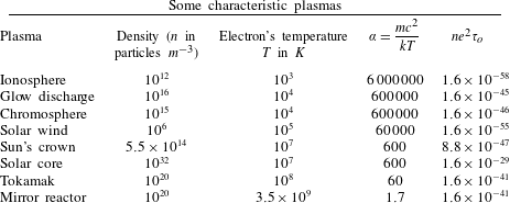
stays small (see table 1 and Riviere (Reference Riviere1971)).
All these different plasmas are such that
 $ne^{2}\unicode[STIX]{x1D70F}_{o}\ll 1$
. Mirror reactor data are from Riviere (Reference Riviere1971).

On the other hand, although the Landau–Lifshitz equation (Landau & Lifshitz Reference Landau and Lifshitz1962) is considered as a first-order approximation in
 $\unicode[STIX]{x1D70F}_{o}$
of the Lorentz–Dirac equation (Dirac Reference Dirac1938), many authors refer to it as the exact equation of motion for a charge particle. Indeed, for Spohn (Reference Spohn2000) and Rohrlich (Reference Rohrlich2000, Reference Rohrlich2001), the Lorentz–Dirac equation must be restricted to its critical surface yielding the Landau–Lifshitz equation and consequently this last one represents the correct equation of motion of a spinless classical point charge. Moreover, by considering a generalized quantum Langevin equation and by giving a structure to the electron with a form factor and a finite cutoff parameter, Ford & O’Connell (Reference Ford and O’Connell1991) derived a non-relativistic equation of motion for charged particles. Generalizing this equation to special relativity (Ford & O’Connell Reference Ford and O’Connell1993), they obtained an equation that Eliezer (Reference Eliezer1948) derived fifty years before using distinct arguments. Although, the Landau–Lifshitz equation and the Eliezer–Ford equation are mathematically different, their physical implications are equivalent (Di Piazza Reference Di Piazza2008; Di Piazza et al.
Reference Di Piazza, Müller, Hatsagortsyan and Keitel2012; Kravets, Noble & Jaroszynski Reference Kravets, Noble and Jaroszynski2013; García-Camacho et al.
Reference García-Camacho, Salinas, Avalos-Vargas and Ares de Parga2015) within Shen’s zone (Shen Reference Shen1972) where quantum effects are negligible. Albeit that the Landau–Lifshitz equation can be considered or not as an approximation at first order in
 $\unicode[STIX]{x1D70F}_{o}$
of the Lorentz–Dirac equation (Dirac Reference Dirac1938), the reality is that the differences with the Lorentz–Dirac equation or with the Eliezer–Ford–O’Connell equation (Eliezer Reference Eliezer1948; Ford & O’Connell Reference Ford and O’Connell1993), are negligible except in the cases of self-accelerations and pre-accelerations (Di Piazza Reference Di Piazza2008; Di Piazza et al.
Reference Di Piazza, Müller, Hatsagortsyan and Keitel2012; Kravets et al.
Reference Kravets, Noble and Jaroszynski2013; García-Camacho et al.
Reference García-Camacho, Salinas, Avalos-Vargas and Ares de Parga2015).
Once the Landau–Lifshitz equation is chosen to describe the motion of the charges, it is necessary to eliminate the degree of freedom represented by considering the hyper-acceleration as an independent variable in the deduction of the density function. Indeed, the hyper-acceleration does not appear anymore. Therefore, we can follow Hakim & Mangeney (Reference Hakim and Mangeney1968) in the deduction of the density just by considering the positions and the velocities of the particles as independent variables. The phase space results in a
 $7N$
-dimensional space (
 $8N-N$
, due to the kinematic relations). The final result coincides with Hakim’s generalization of the Vlasov equation in special relativity (Hakim & Mangeney Reference Hakim and Mangeney1968) giving, by a linearization process, the same dispersion relations. Moreover, in appendix A, a more general equation is deduced by including a constant external weak electric field. The dispersion relations are obtained for this case and the effects of the coupling between the constant external weak electric field and the interaction of the particle do not play an important role. The dispersion relations are not affected despite having very large Debye length at relativistic temperatures. Moreover, the LD can be deduced and compared with the RRFD. By giving an expansion in terms of
 $\unicode[STIX]{x1D707}=w/ck$
(
 $\unicode[STIX]{x1D707}\geqslant 1$
or
 $\unicode[STIX]{x1D707}<1$
) in the integrals involved in the dispersion relations, a general expression for the wave dispersion relations for the longitudinal mode can be expressed in order to give numerical solutions.
It has to be highlighted that in many articles these dispersion relations have been studied for different relativistic cases; such as for examples, hot relativistic beam–plasma systems (Magneville Reference Magneville1990), the one-dimensional tearing mode equation in tokamaks (Jovanović & Dimitrijević Reference Jovanović and Dimitrijević2013), the nonlinear case but at moderate plasma temperature (Pesch & Kull Reference Pesch and Kull2010). the nonlinear case of large amplitude electromagnetic waves coupled with electrostatic waves (Connor et al.
Reference Connor, Hastie, Marchetto and Roach2018) and the one-dimensional linear longitudinal case (Zhang et al.
Reference Zhang, Wu, Zhou, Zhu and He2013). Particularly, the work done by Zhang et al. (Reference Zhang, Wu, Zhou, Zhu and He2013) describes the relativistic dispersion relations for longitudinal modes in a one-dimensional model and it is an excellent opportunity to compare the latter with the dispersion relations obtained in this covariant approach where the magnetic field generated by the relativistic motions of the electrons is taken into account. Indeed, this procedure must give different results due to two reasons: the first one, as we noticed before, is related to the fact that the magnetic field generated by high velocity electrons must be considered; the second consists of using the covariant
 $4$
-dimension Jüttner distribution function (Jüttner Reference Jüttner1911; Synge Reference Synge1956; Cubero et al.
Reference Cubero, Casado-Pascual, Dunkel, Talkner and Hänggi2007; López-Carrera & Ares de Parga Reference López-Carrera and Ares de Parga2008). It has to be pointed out that in this paper a correct expansion is done in terms of
 $\unicode[STIX]{x1D707}$
(
 $\unicode[STIX]{x1D707}\geqslant 1$
or
 $\unicode[STIX]{x1D707}<1$
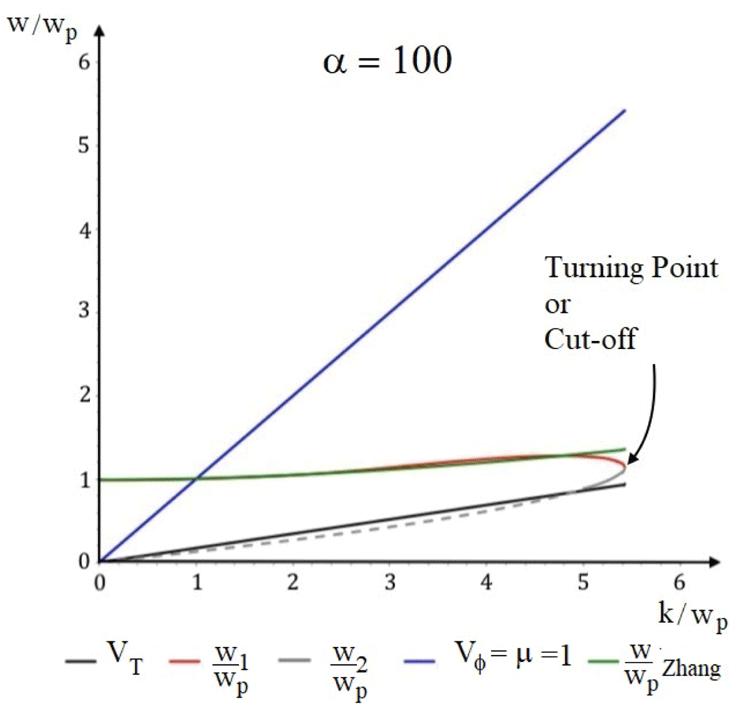
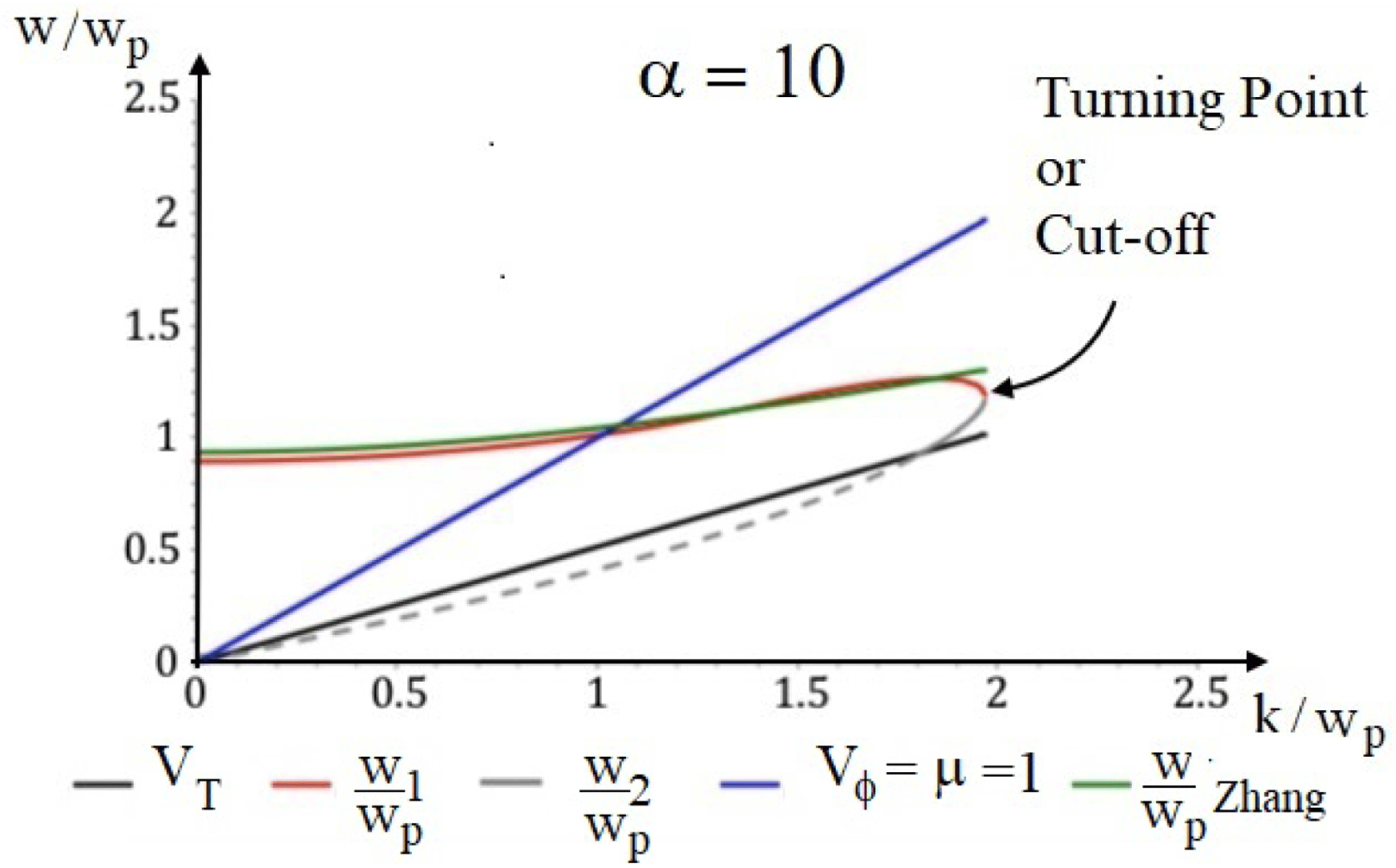
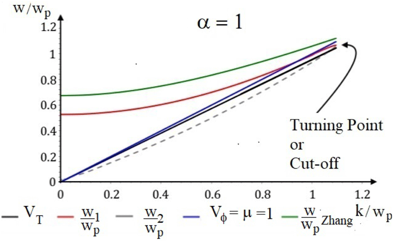
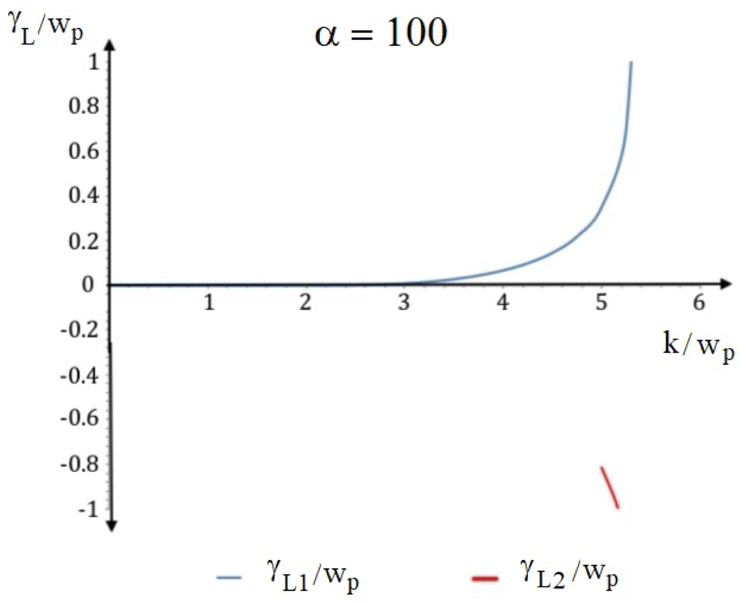
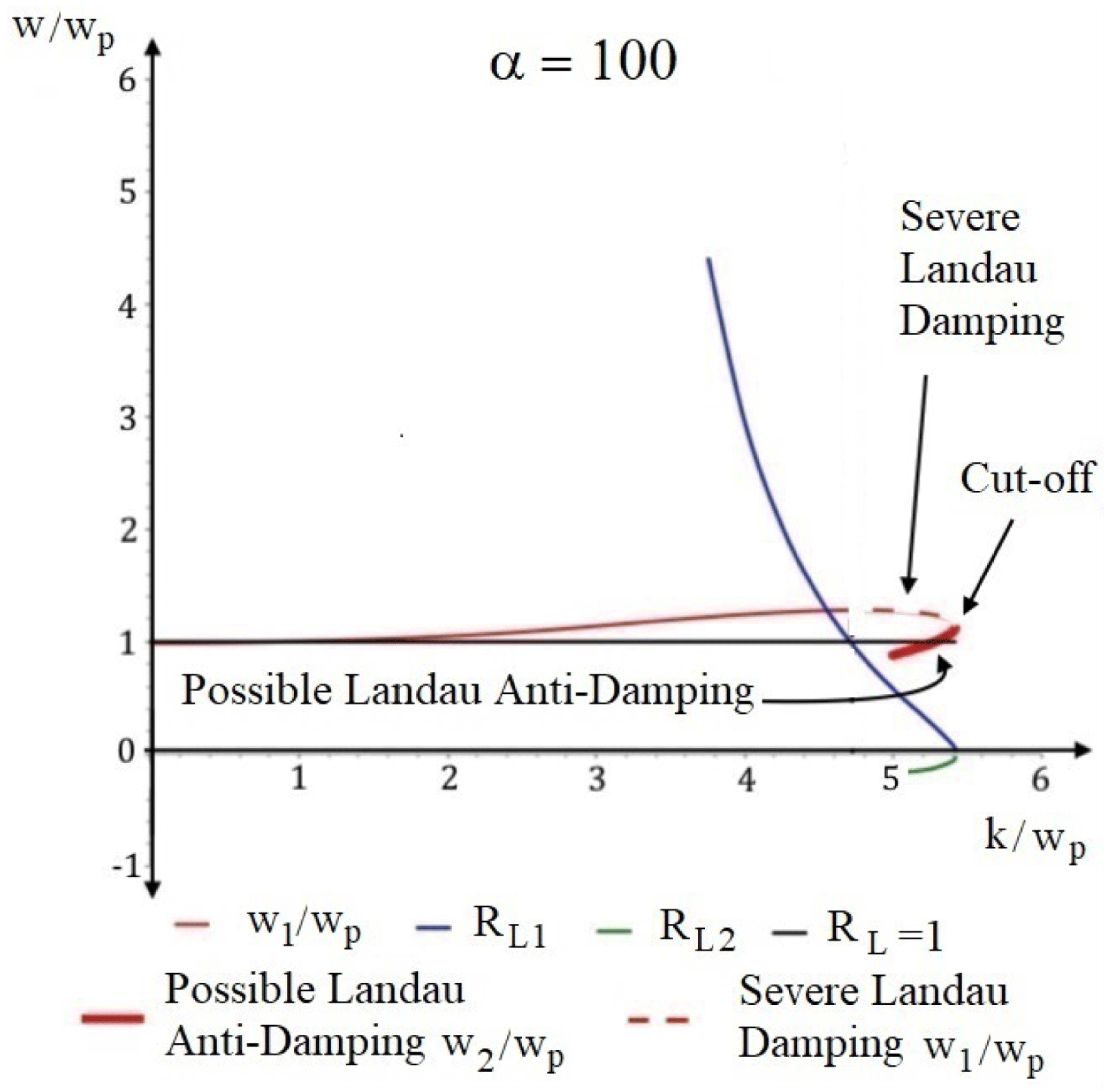
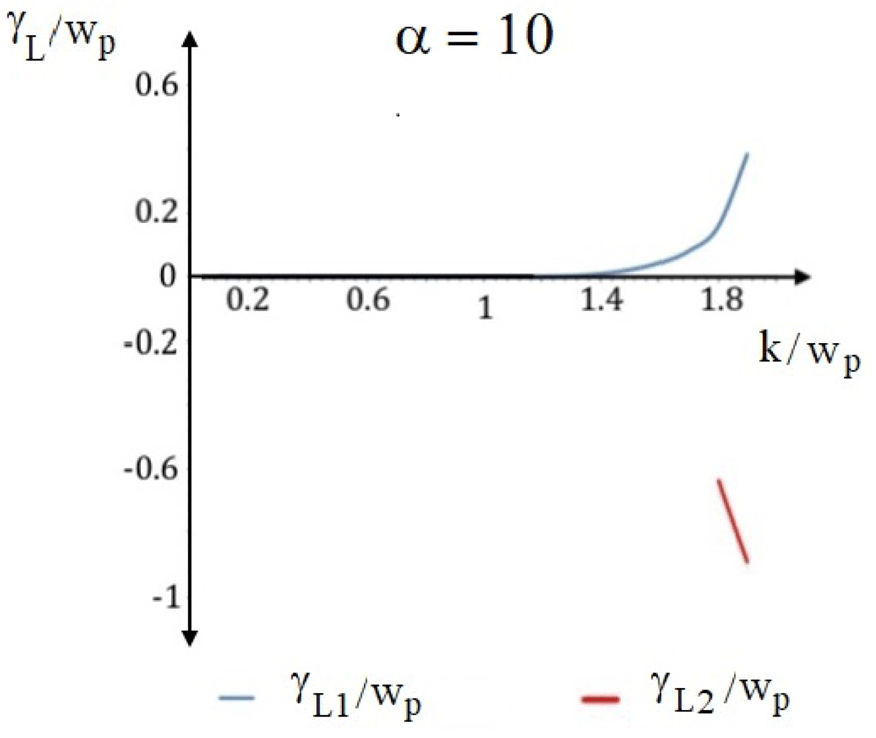
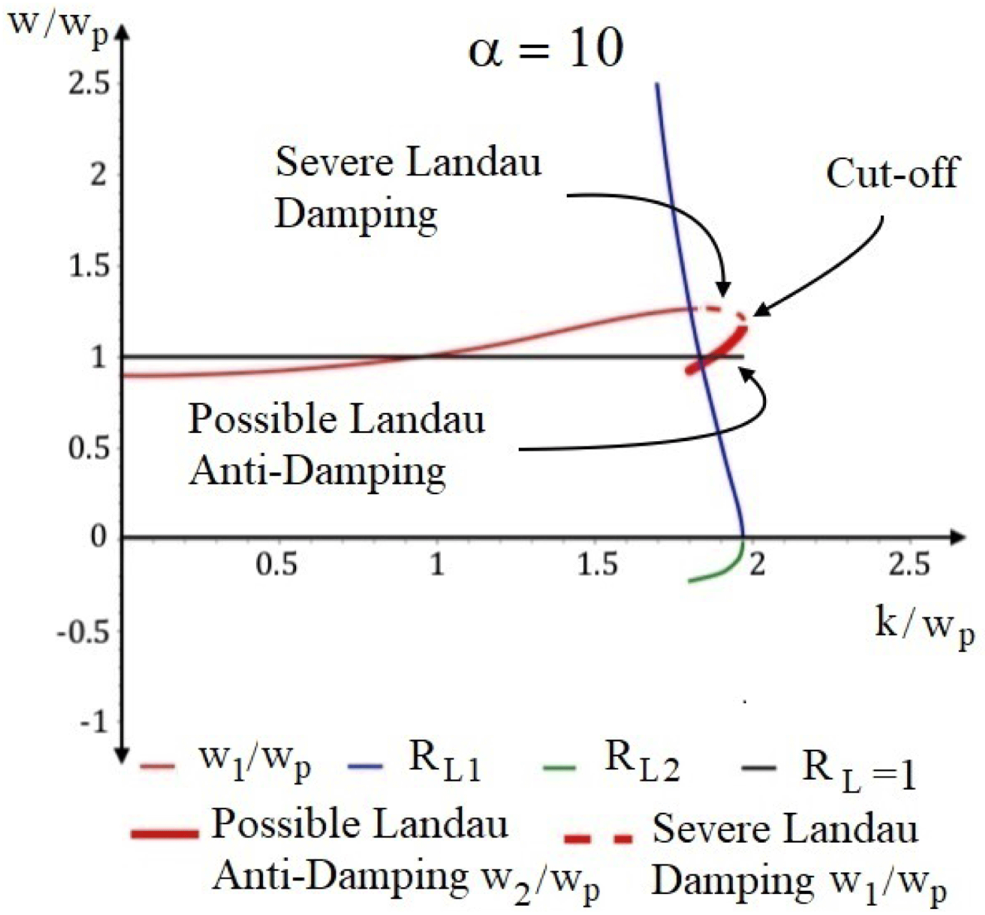
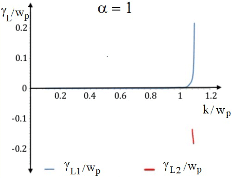
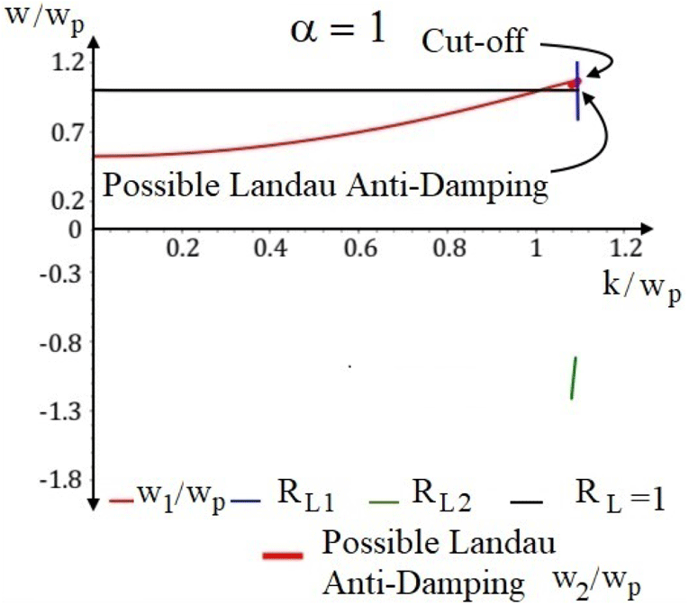
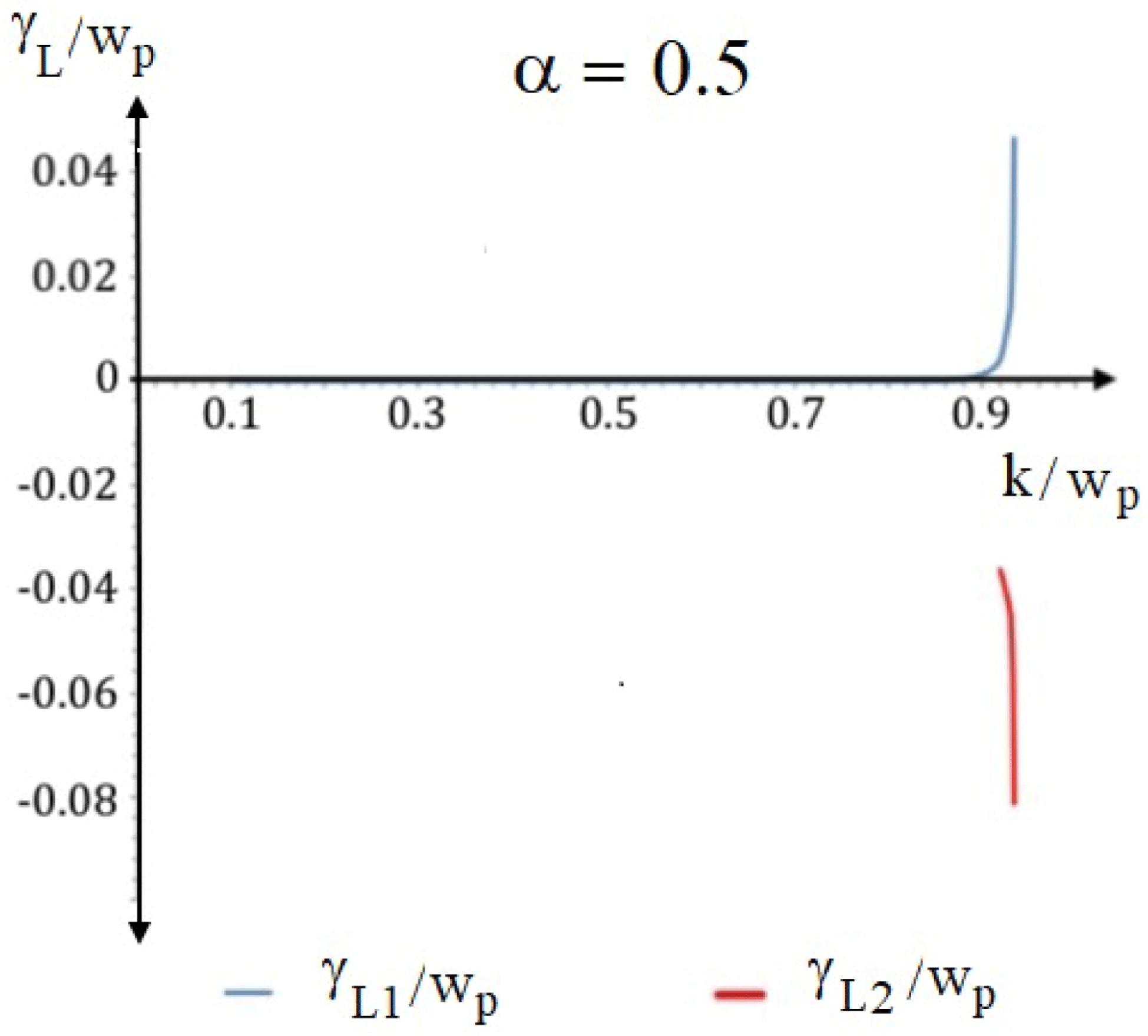
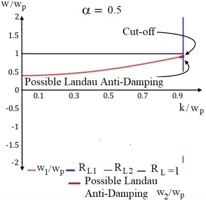
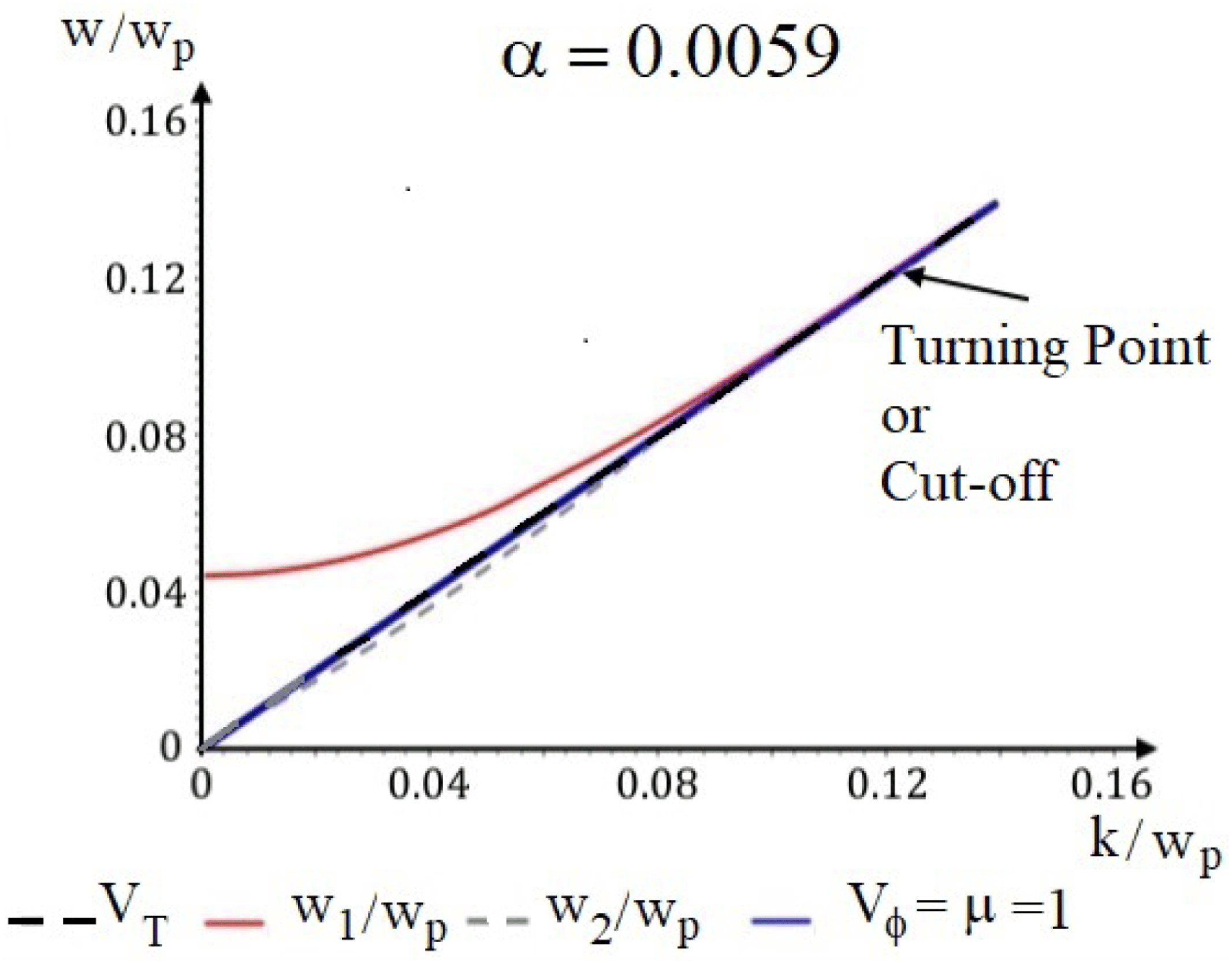
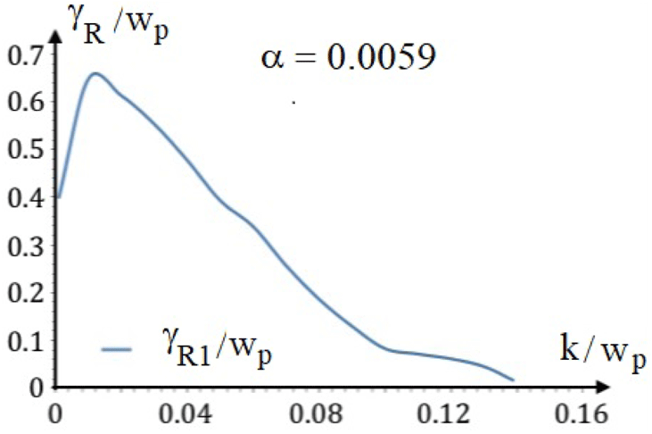
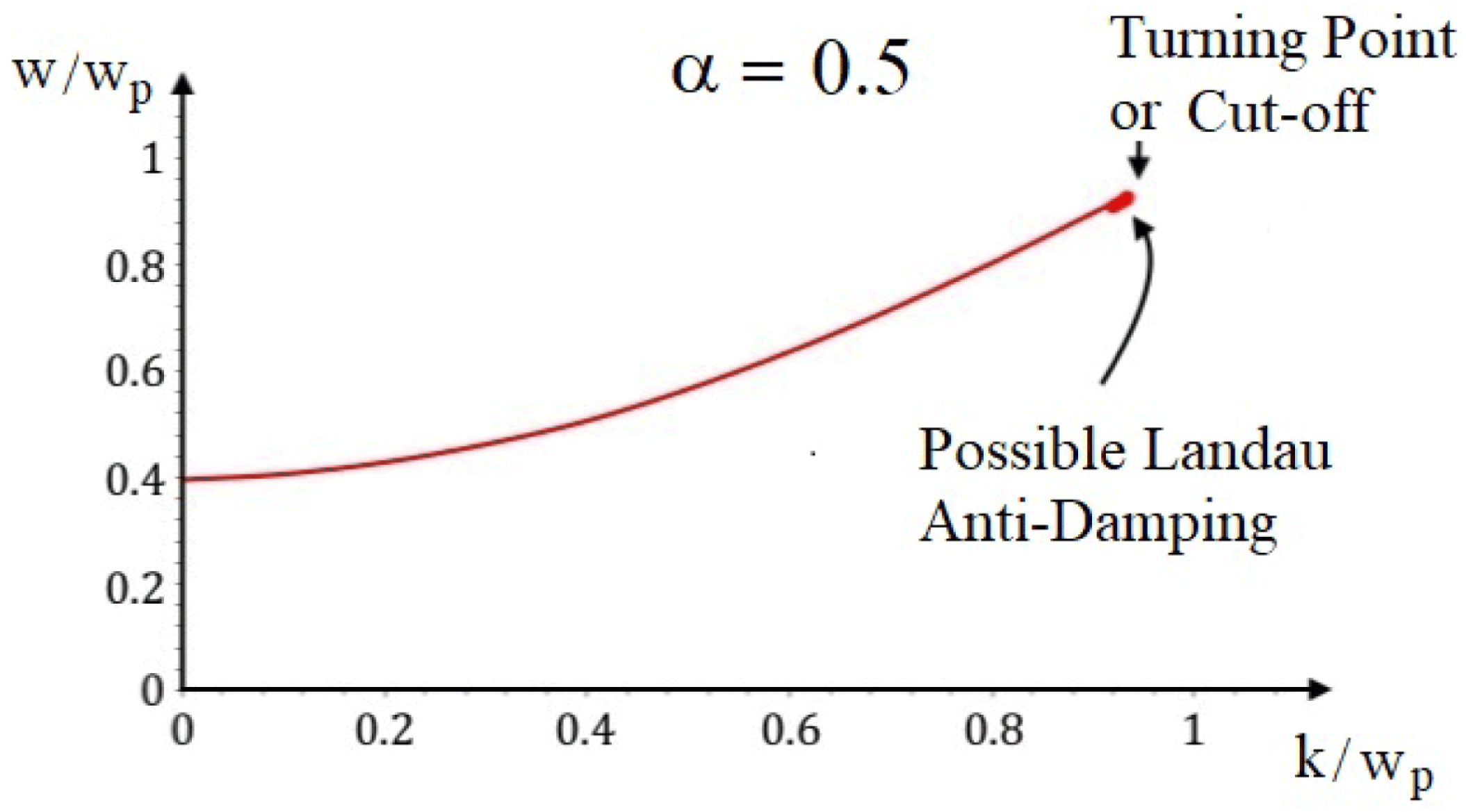
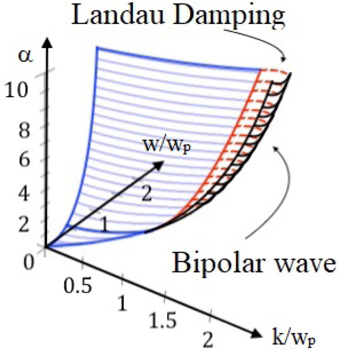
) in order to be able to calculate some integrals which appear in the dispersion relations, giving new loop types of solutions crossing the super-luminous region and the super-thermal region (two branches). The interesting result is that a cutoff for the wave appears for any value of the temperature. The LD vanishes in the super-luminous region as Hakim and Mangeney, and Zhang predicted (Hakim & Mangeney Reference Hakim and Mangeney1971; Zhang et al.
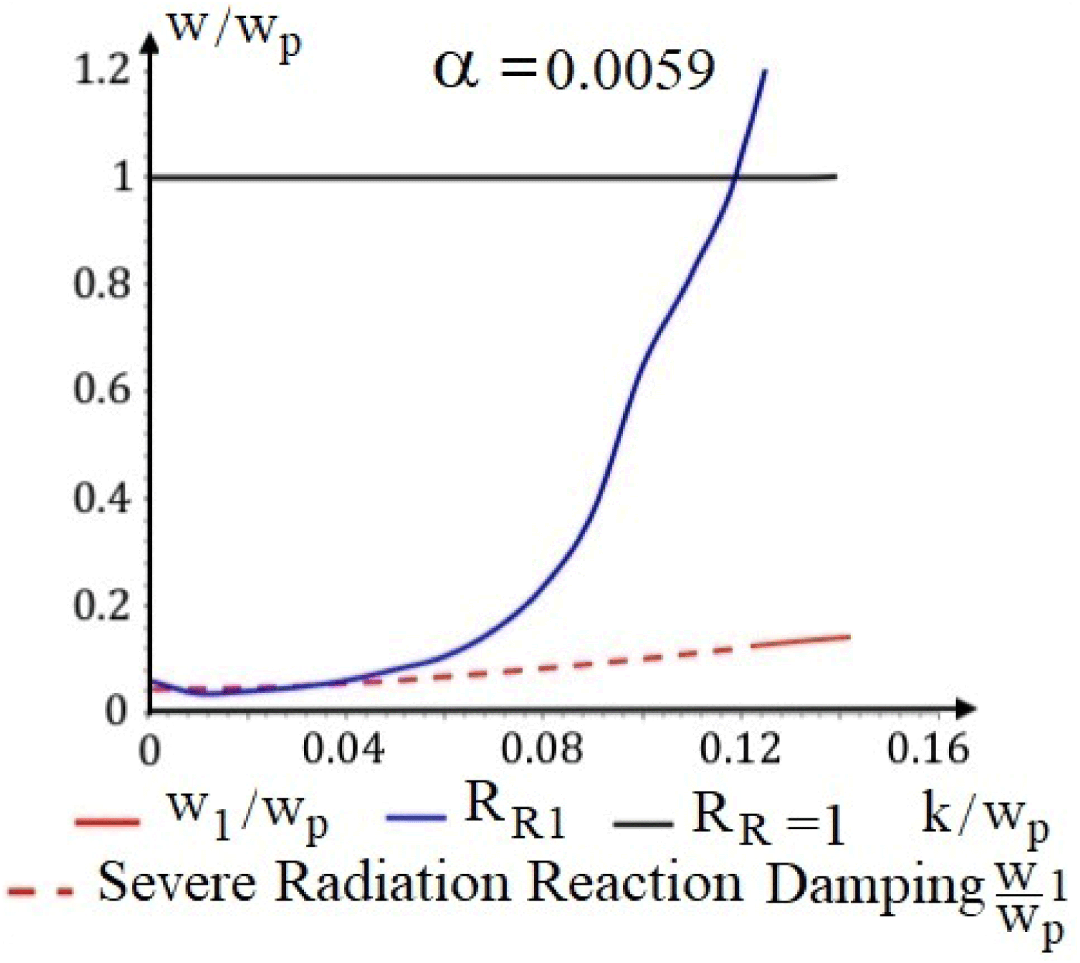
Reference Zhang, Wu, Zhou, Zhu and He2013). However, for the super-thermal region after the cutoff, that is in the second branch, the LD turns to be an anti-damping and possible resonance may appear. However, those possible anti-damping solutions are near to the damping solutions with different close temperatures. Indeed, the perturbation heats locally the plasma in such a way that the temperature cannot be considered as exact data and the wave suffers an anti-damping and a damping during a short period or disappears due to the cutoff. Therefore, those solutions will be called bipolar waves. This represents a novel result which is due to the existence of the second branch. For the RRFD, our general expression differs from the one obtained by Hakim & Mangeney (Reference Hakim and Mangeney1968, Reference Hakim and Mangeney1971) giving distinct behaviour of the damping. Indeed, the RRFD of Hakim and Mangeney is proportional to
 $w/k$
which permits us to obtain strong damping for high temperatures. However, our result neglects such important damping unless the plasma frequency is so high that the density and the temperature are close to the degenerate case and the Hagedorn temperature. The result to highlight is to show that the wave has a cutoff due to the dispersion relations and not due to the RRFD when the densities are low. The RRFD is important when high densities and temperatures are present.
The purpose of this paper is threefold: first, a deduction of a modified covariant relativistic Vlasov equation which includes the effect of the radiation reaction force in the plasma by using the Landau–Lifshitz equation. General dispersion relations are obtained for transverse and longitudinal modes; second, by making an exact expansion in terms of
 $\unicode[STIX]{x1D707}$
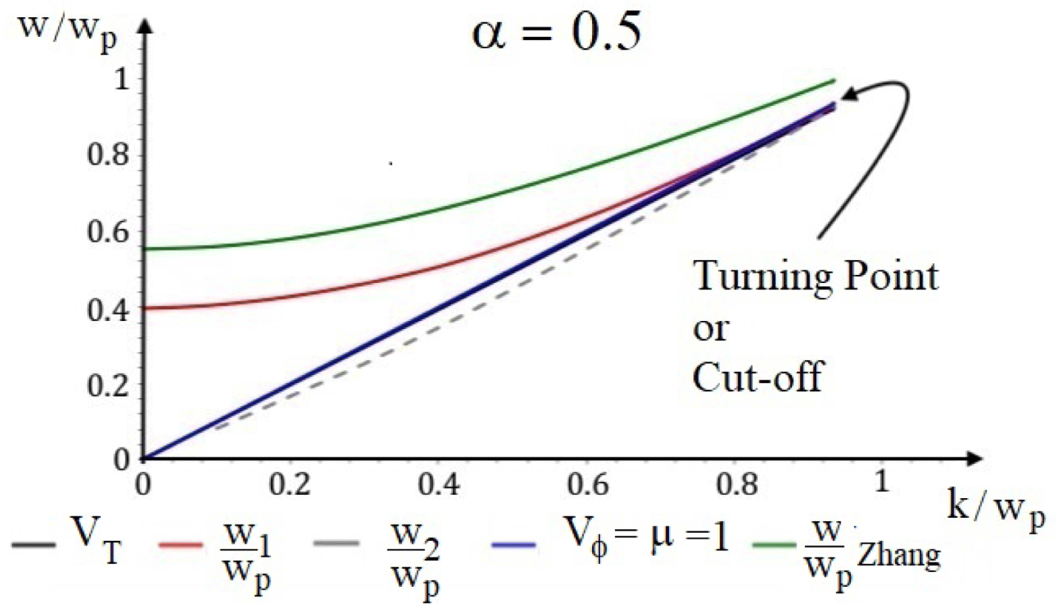
, numerically relations are described showing the shift of the plasma frequency, the existence of loop solutions (two branches with a turning point) crossing the super-luminous region and the super-thermal region, the difference with the Zhang model and the cutoff of the wave for a certain value of the wavenumber
 $k$
which depends on the parameter
 $\unicode[STIX]{x1D6FC}$
(
 $\unicode[STIX]{x1D6FC}$
is related to the inverse of the temperature); third, for the longitudinal mode, general expressions for the LD and the RRFD are obtained and the decay or growth of the waves due to these effects is analysed for different cases.
The article is organized as follows: in § 2, the modified Vlasov equation including the reaction force and an external weak constant electric field is derived. In § 3, the dispersion relations are derived for both transverse and longitudinal modes. The case of an external constant weak electric field is analysed in appendix A given the same dispersion relations. In § 4, the relativistic dispersion relations are expressed by using an expansion in terms of
 $\unicode[STIX]{x1D707}$
inside some integrals that appear in the dispersion relations and this permits us to describe numerically the dispersion relations and to compare them with the results obtained by Zhang et al. (Reference Zhang, Wu, Zhou, Zhu and He2013). Interesting cutoffs of the waves due to the existence of loop solutions with two branches crossing the super-luminous region and the super-thermal region are described. The decay of the waves due to the LD and the RRFD is taken into account to describe the final waves. In § 5, we provide a summary. Some concluding remarks are given in § 6.
2 The modified Vlasov equation including the radiation reaction force and an external weak constant electric field
In order to derive a relativistic modified Vlasov equation which includes the radiation reaction force and an external weak constant electric field, we will use the Landau–Lifshitz equation of motion. It is necessary to describe it for a system of
 $N$
charges. We limit our attention only to a system of electrons because the action of the ions are neglected. This implies that we deal with the constraint in the paper that the thermal velocity
 $V_{Te}$
is smaller than the phase velocity
 $V_{\unicode[STIX]{x1D719}}=w/ck=\unicode[STIX]{x1D707}$
,
 $V_{Ti}\leqslant V_{Te}<V_{\unicode[STIX]{x1D719}}$
.
2.1 Landau–Lifshitz equation
For a system of
 $N$
charged particles with the same mass
 $m$
and equal charge
 $e$
, for each particle the Lorentz–Dirac equation (Dirac Reference Dirac1938) is
 $$\begin{eqnarray}\displaystyle ma_{i}^{\unicode[STIX]{x1D707}}=\frac{e}{c}\unicode[STIX]{x1D641}_{(i)}^{\unicode[STIX]{x1D707}\unicode[STIX]{x1D708}}v_{\unicode[STIX]{x1D708}i}+m\unicode[STIX]{x1D70F}_{o}\left[{\dot{a}}_{i}^{\unicode[STIX]{x1D707}}+\frac{a_{i}^{2}}{c^{2}}v_{i}^{\unicode[STIX]{x1D707}}\right],\quad i=1,\ldots ,N, & & \displaystyle\end{eqnarray}$$
where
 $c$
,
 $\unicode[STIX]{x1D641}_{(i)}^{\unicode[STIX]{x1D707}\unicode[STIX]{x1D708}}$
and
 $\unicode[STIX]{x1D70F}_{o}=2e^{2}/3mc^{3}$
are the speed of light, the field strength tensor due to the action of the other particles, the external field on the
 $i$
th particle and the characteristic time of the charge
 $e$
, respectively. The subscript ‘
 $i$
’ represents the
 $i$
th particle and
 $v_{i}^{\unicode[STIX]{x1D707}}$
,
 $a_{i}^{\unicode[STIX]{x1D707}}$
and
 ${\dot{a}}_{i}^{\unicode[STIX]{x1D707}}=\text{d}a_{i}^{\unicode[STIX]{x1D707}}/\text{d}\unicode[STIX]{x1D70F}_{i}$
are the
 $4$
-velocity, the
 $4$
-acceleration and the
 $4$
-hyper-acceleration of the
 $i$
th particle, respectively, with
 $\unicode[STIX]{x1D70F}_{i}$
the proper time of the
 $i$
th particle. The equation can be expressed as
 $$\begin{eqnarray}\displaystyle ma_{i}^{\unicode[STIX]{x1D707}}=\frac{e}{c}\unicode[STIX]{x1D641}_{(i)}^{\unicode[STIX]{x1D707}\unicode[STIX]{x1D708}}v_{\unicode[STIX]{x1D708}i}+m\unicode[STIX]{x1D70F}_{o}\unicode[STIX]{x1D6E5}^{\unicode[STIX]{x1D707}\unicode[STIX]{x1D708}}(v_{i}){\dot{a}}_{\unicode[STIX]{x1D708}i},\quad i=1,\ldots ,N, & & \displaystyle\end{eqnarray}$$
where
 $$\begin{eqnarray}\displaystyle \unicode[STIX]{x1D6E5}^{\unicode[STIX]{x1D707}\unicode[STIX]{x1D708}}(v_{i})=g^{\unicode[STIX]{x1D707}\unicode[STIX]{x1D708}}-\frac{v_{i}^{\unicode[STIX]{x1D707}}v_{i}^{\unicode[STIX]{x1D708}}}{c^{2}}, & & \displaystyle\end{eqnarray}$$
with
 $g^{\unicode[STIX]{x1D707}\unicode[STIX]{x1D708}}$
representing the Minkowski metric and the kinematic relation
 $v^{\unicode[STIX]{x1D707}}{\dot{a}}_{\unicode[STIX]{x1D707}}+a^{\unicode[STIX]{x1D707}}a_{\unicode[STIX]{x1D707}}=0$
has been used. In order to incorporate the Landau–Lifshitz proposal in (2.2), the hyper-acceleration must be substituted by
 $$\begin{eqnarray}\displaystyle {\dot{a}}_{\unicode[STIX]{x1D708}i}\rightarrow \frac{e}{mc}\frac{\text{d}}{\text{d}\unicode[STIX]{x1D70F}_{i}}\unicode[STIX]{x1D641}_{\unicode[STIX]{x1D708}\unicode[STIX]{x1D6FC}}^{(i)}v_{i}^{\unicode[STIX]{x1D6FC}}=\frac{e}{mc}\left[\unicode[STIX]{x1D641}_{\unicode[STIX]{x1D708}\unicode[STIX]{x1D6FC}}^{(i)}a_{i}^{\unicode[STIX]{x1D6FC}}+v_{i}^{\unicode[STIX]{x1D70C}}v_{i}^{\unicode[STIX]{x1D6FC}}\frac{\unicode[STIX]{x2202}\unicode[STIX]{x1D641}_{\unicode[STIX]{x1D708}\unicode[STIX]{x1D6FC}}^{(i)}}{\unicode[STIX]{x2202}x_{i}^{\unicode[STIX]{x1D70C}}}\right], & & \displaystyle\end{eqnarray}$$
and in a second step, in the first term of the right-hand side of (2.4), the acceleration
 $a_{i}^{\unicode[STIX]{x1D6FC}}$
, must be substituted by the Lorentz force; that is:
 $$\begin{eqnarray}\displaystyle {\dot{a}}_{\unicode[STIX]{x1D708}i}\rightarrow \frac{e}{mc}\left[\frac{e}{mc}\unicode[STIX]{x1D641}_{\unicode[STIX]{x1D708}\unicode[STIX]{x1D6FC}}^{(i)}\unicode[STIX]{x1D641}_{(i)}^{\unicode[STIX]{x1D6FC}\unicode[STIX]{x1D6FD}}v_{\unicode[STIX]{x1D6FD}i}+v_{i}^{\unicode[STIX]{x1D70C}}v_{i}^{\unicode[STIX]{x1D6FC}}\frac{\unicode[STIX]{x2202}\unicode[STIX]{x1D641}_{\unicode[STIX]{x1D708}\unicode[STIX]{x1D6FC}}^{(i)}}{\unicode[STIX]{x2202}x_{i}^{\unicode[STIX]{x1D70C}}}\right]. & & \displaystyle\end{eqnarray}$$
Therefore, the Landau–Lifshitz equation of motion for each particle is (Ares de Parga Reference Ares de Parga2006)
 $i=1,\ldots ,N,$
 $$\begin{eqnarray}\displaystyle ma_{i}^{\unicode[STIX]{x1D707}}=\frac{e}{c}\unicode[STIX]{x1D641}_{(i)}^{\unicode[STIX]{x1D707}\unicode[STIX]{x1D708}}v_{\unicode[STIX]{x1D708}i}+m\unicode[STIX]{x1D70F}_{o}\unicode[STIX]{x1D6E5}^{\unicode[STIX]{x1D707}\unicode[STIX]{x1D708}}(v_{i})\frac{e}{mc}\left[\frac{e}{mc}\unicode[STIX]{x1D641}_{\unicode[STIX]{x1D708}\unicode[STIX]{x1D6FC}}^{(i)}\unicode[STIX]{x1D641}_{(i)}^{\unicode[STIX]{x1D6FC}\unicode[STIX]{x1D6FD}}v_{\unicode[STIX]{x1D6FD}i}+v_{i}^{\unicode[STIX]{x1D70C}}v_{i}^{\unicode[STIX]{x1D6FC}}\frac{\unicode[STIX]{x2202}\unicode[STIX]{x1D641}_{\unicode[STIX]{x1D708}\unicode[STIX]{x1D6FC}}^{(i)}}{\unicode[STIX]{x2202}x_{i}^{\unicode[STIX]{x1D70C}}}\right]. & & \displaystyle\end{eqnarray}$$
On the other hand, the force applied on each particle must be decomposed into two parts: the external field and the field produced by the other particles on the
 $i$
th particle; that is
 $$\begin{eqnarray}\displaystyle \unicode[STIX]{x1D641}_{(i)}^{\unicode[STIX]{x1D707}\unicode[STIX]{x1D708}}=\unicode[STIX]{x1D641}_{\text{ext}}^{\unicode[STIX]{x1D707}\unicode[STIX]{x1D708}}+\mathop{\sum }_{j\neq i}\unicode[STIX]{x1D641}_{ji}^{\unicode[STIX]{x1D707}\unicode[STIX]{x1D708}}(x_{\unicode[STIX]{x1D70C}}), & & \displaystyle\end{eqnarray}$$
where
 $$\begin{eqnarray}\displaystyle \unicode[STIX]{x1D641}_{ji}^{\unicode[STIX]{x1D707}\unicode[STIX]{x1D708}}(x_{\unicode[STIX]{x1D70C}}) & = & \displaystyle \frac{4\unicode[STIX]{x03C0}e}{c}\iiint \text{d}^{4}x^{\prime }\,\text{d}^{4}v^{\prime }\,\text{d}\unicode[STIX]{x1D70F}^{\prime }[v^{\prime \unicode[STIX]{x1D708}}\unicode[STIX]{x2202}^{\unicode[STIX]{x1D707}}-v^{\prime \unicode[STIX]{x1D707}}\unicode[STIX]{x2202}^{\unicode[STIX]{x1D708}}]D_{\text{ret}}(x_{\unicode[STIX]{x1D70C}}-x_{\unicode[STIX]{x1D70C}}^{\prime })\nonumber\\ \displaystyle & & \displaystyle \times \,\unicode[STIX]{x1D6FF}(x_{\unicode[STIX]{x1D70C}}^{\prime }-x_{\unicode[STIX]{x1D70C}j}(\unicode[STIX]{x1D70F}^{\prime }))\unicode[STIX]{x1D6FF}(v_{\unicode[STIX]{x1D70C}}^{\prime }-v_{\unicode[STIX]{x1D70C}j}(\unicode[STIX]{x1D70F}^{\prime })),\end{eqnarray}$$
where
 $D_{\text{ret}}$
represents the retarded Green function (Jackson Reference Jackson1998).
Finally, it is important to note that the equation of motion described by (2.6) does not depend on the hyper-acceleration and consequently the phase space is described by a
 $8N$
-dimensional space with the regular
 $N$
constraint,
 $v^{\unicode[STIX]{x1D707}}v_{\unicode[STIX]{x1D707}}=c^{2}$
. This point represents one of the different approaches to obtaining the relativistic Vlasov equation compared with the work done by Hakim & Mangeney (Reference Hakim and Mangeney1968).
2.2 Relativistic Vlasov equation including radiation reaction force
Different derivations of a hierarchy of statistical equations were developed during the last century, independently, by Bogolyubov, Born and Green, Kirkwood and Yvon (the so-called BBGKY hierarchy). Particularly, we can cite the work done by Bogolyubov (Reference Bogolyubov1946) in the early sixties. An important approach was done by Hakim I (Reference Hakim1967), Hakim II (Reference Hakim1967) which lead to a hierarchy of manifestly covariant equations for a system of charge particles including the radiation reaction force (Hakim & Mangeney Reference Hakim and Mangeney1968, Reference Hakim and Mangeney1971) with the constraint of the absence of any correlation between the particles and equations to first order in
 $ne^{2}\unicode[STIX]{x1D70F}_{o}$
. We will follow Hakim and Mangeney in order to obtain a relativistic covariant modified Vlasov equation but with the difference that we will start from a phase space without the hyper-acceleration as an independent variable and including a weak constant electric field. The fact of not considering the hyper-acceleration as an independent variable is because we consider the Landau–Lifshitz equation of motion, which does not contain such dependence.
Let us make a summary of the derivation of the modified Vlasov equation just to place emphasis on the differences between our method and the Hakim and Mangeney one. The phase space in special relativity must be constructed by following the dynamics of the particles in the system. By looking at the equation of motion, equation (2.6), it is clear that the phase space is composed of
 $$\begin{eqnarray}\displaystyle \unicode[STIX]{x1D6E4}={\{x_{\unicode[STIX]{x1D707}}\}}^{N}\times {\{v_{\unicode[STIX]{x1D707}}\}}^{N}, & & \displaystyle\end{eqnarray}$$
accompanied by the constraint
 $$\begin{eqnarray}\displaystyle v_{\unicode[STIX]{x1D707}}v^{\unicode[STIX]{x1D707}}=c^{2}, & & \displaystyle\end{eqnarray}$$
which can be incorporated directly in the densities by using a delta function. Notice that unlike Hakim & Mangeney (Reference Hakim and Mangeney1968) the hyper-acceleration is not taken as part of the phase space since the equation of motion to be considered is the Landau–Lifshitz equation which is a second-order differential equation. Using the regular assumptions of the Gibbs ensemble (Hakim I Reference Hakim1967; Hakim II Reference Hakim1967), it is possible to define a random one-particle density as
 $$\begin{eqnarray}\displaystyle R_{1}(x_{\unicode[STIX]{x1D707}},v_{\unicode[STIX]{x1D707}};\unicode[STIX]{x1D70F})=\mathop{\sum }_{i=1}^{N}\unicode[STIX]{x1D6FF}(x_{\unicode[STIX]{x1D707}}-x_{\unicode[STIX]{x1D707}i}(\unicode[STIX]{x1D70F}))\unicode[STIX]{x1D6FF}(v_{\unicode[STIX]{x1D707}}-v_{\unicode[STIX]{x1D707}i}(\unicode[STIX]{x1D70F})), & & \displaystyle\end{eqnarray}$$
where
 $\unicode[STIX]{x1D70F}$
represents a parameter which will describe the trajectory of each particle by means of
 $v_{\unicode[STIX]{x1D707}i}(\unicode[STIX]{x1D70F})=\text{d}x_{\unicode[STIX]{x1D707}i}(\unicode[STIX]{x1D70F})/\text{d}\unicode[STIX]{x1D70F}$
. Also, following Hakim & Mangeney (Reference Hakim and Mangeney1968), we define the proper time-dependent density,
 $$\begin{eqnarray}\displaystyle D_{1}(x_{\unicode[STIX]{x1D707}},v_{\unicode[STIX]{x1D707}};\unicode[STIX]{x1D70F})=N\langle R_{1}(x_{\unicode[STIX]{x1D707}},v_{\unicode[STIX]{x1D707}};\unicode[STIX]{x1D70F})\rangle , & & \displaystyle\end{eqnarray}$$
where the brackets
 $\langle R_{1}\rangle$
represent the regular average weighted by random initial conditions (Hakim I Reference Hakim1967; Hakim II Reference Hakim1967). Also, we will need
 $$\begin{eqnarray}\displaystyle R_{2}(x_{\unicode[STIX]{x1D707}},v_{\unicode[STIX]{x1D707}},\unicode[STIX]{x1D70F};x_{\unicode[STIX]{x1D707}}^{\prime },v_{\unicode[STIX]{x1D707}}^{\prime },\unicode[STIX]{x1D70F}^{\prime }) & = & \displaystyle \mathop{\sum }_{i\neq j}\unicode[STIX]{x1D6FF}(x_{\unicode[STIX]{x1D707}}-x_{\unicode[STIX]{x1D707}i}(\unicode[STIX]{x1D70F}))\nonumber\\ \displaystyle & & \displaystyle \times \,\unicode[STIX]{x1D6FF}(v_{\unicode[STIX]{x1D707}}-v_{\unicode[STIX]{x1D707}i}(\unicode[STIX]{x1D70F}))\unicode[STIX]{x1D6FF}(x_{\unicode[STIX]{x1D707}}^{\prime }-x_{\unicode[STIX]{x1D707}i}(\unicode[STIX]{x1D70F}^{\prime }))\unicode[STIX]{x1D6FF}(v_{\unicode[STIX]{x1D707}}^{\prime }-v_{\unicode[STIX]{x1D707}i}(\unicode[STIX]{x1D70F}^{\prime })),\quad\end{eqnarray}$$
and
 $$\begin{eqnarray}\displaystyle D_{2}=(x_{\unicode[STIX]{x1D707}},v_{\unicode[STIX]{x1D707}},\unicode[STIX]{x1D70F};x_{\unicode[STIX]{x1D707}}^{\prime },v_{\unicode[STIX]{x1D707}}^{\prime },\unicode[STIX]{x1D70F}^{\prime })=N(N-1)\langle R_{2}(x_{\unicode[STIX]{x1D707}},v_{\unicode[STIX]{x1D707}},\unicode[STIX]{x1D70F};x_{\unicode[STIX]{x1D707}}^{\prime },v_{\unicode[STIX]{x1D707}}^{\prime },\unicode[STIX]{x1D70F}^{\prime })\rangle . & & \displaystyle\end{eqnarray}$$
Finally, the relativistic one-particle density is
 $$\begin{eqnarray}\displaystyle {\mathcal{N}}_{1}(x_{\unicode[STIX]{x1D707}},v_{\unicode[STIX]{x1D707}})=\int _{-\infty }^{\infty }D_{1}(x_{\unicode[STIX]{x1D707}},v_{\unicode[STIX]{x1D707}};\unicode[STIX]{x1D70F})\,\text{d}\unicode[STIX]{x1D70F}. & & \displaystyle\end{eqnarray}$$
In order to obtain the continuity equation, let us follow the Klimontovich method (Klimontovich Reference Klimontovich1960), but with a difference since the force on each particle will not be the Lorentz force but the Lorentz force plus the radiation reaction force due to Landau and Lifshitz represented by (2.6). Starting from equation (2.11) in the equivalent following form
 $$\begin{eqnarray}\displaystyle R_{1}(x^{\unicode[STIX]{x1D707}},v^{\unicode[STIX]{x1D707}};\unicode[STIX]{x1D70F})=\mathop{\sum }_{i=1}^{N}\unicode[STIX]{x1D6FF}(x^{\unicode[STIX]{x1D707}}-x_{i}^{\unicode[STIX]{x1D707}}(\unicode[STIX]{x1D70F}))\unicode[STIX]{x1D6FF}(v^{\unicode[STIX]{x1D707}}-v_{i}^{\unicode[STIX]{x1D707}}(\unicode[STIX]{x1D70F})), & & \displaystyle\end{eqnarray}$$
and partially differentiating it with respect to
 $\unicode[STIX]{x1D70F}$
, we have,
 $$\begin{eqnarray}\displaystyle \frac{\unicode[STIX]{x2202}R_{1}(x^{\unicode[STIX]{x1D707}},v^{\unicode[STIX]{x1D707}};\unicode[STIX]{x1D70F})}{\unicode[STIX]{x2202}\unicode[STIX]{x1D70F}} & = & \displaystyle \mathop{\sum }_{i=1}^{N}\left\{\frac{\unicode[STIX]{x2202}}{\unicode[STIX]{x2202}\unicode[STIX]{x1D70F}}\unicode[STIX]{x1D6FF}(x^{\unicode[STIX]{x1D707}}-x_{i}^{\unicode[STIX]{x1D707}}(\unicode[STIX]{x1D70F}))\right\}\unicode[STIX]{x1D6FF}(v^{\unicode[STIX]{x1D707}}-v_{i}^{\unicode[STIX]{x1D707}}(\unicode[STIX]{x1D70F}))\nonumber\\ \displaystyle & & \displaystyle +\,\unicode[STIX]{x1D6FF}(x^{\unicode[STIX]{x1D707}}-x_{i}^{\unicode[STIX]{x1D707}}(\unicode[STIX]{x1D70F}))\left\{\frac{\unicode[STIX]{x2202}}{\unicode[STIX]{x2202}\unicode[STIX]{x1D70F}}\unicode[STIX]{x1D6FF}(v^{\unicode[STIX]{x1D707}}-v_{i}^{\unicode[STIX]{x1D707}}(\unicode[STIX]{x1D70F}))\right\}\nonumber\\ \displaystyle & = & \displaystyle \mathop{\sum }_{i=1}^{N}\left\{-\frac{\text{d}x_{i}^{\unicode[STIX]{x1D707}}(\unicode[STIX]{x1D70F})}{\text{d}\unicode[STIX]{x1D70F}}\frac{\unicode[STIX]{x2202}}{\unicode[STIX]{x2202}x^{\unicode[STIX]{x1D707}}}\unicode[STIX]{x1D6FF}(x^{\unicode[STIX]{x1D707}}-x_{i}^{\unicode[STIX]{x1D707}}(\unicode[STIX]{x1D70F}))\right\}\unicode[STIX]{x1D6FF}(v^{\unicode[STIX]{x1D707}}-v_{i}^{\unicode[STIX]{x1D707}}(\unicode[STIX]{x1D70F}))\nonumber\\ \displaystyle & & \displaystyle +\,\mathop{\sum }_{i=1}^{N}\unicode[STIX]{x1D6FF}(x^{\unicode[STIX]{x1D707}}-x_{i}^{\unicode[STIX]{x1D707}}(\unicode[STIX]{x1D70F}))\left\{-\frac{\text{d}v_{i}^{\unicode[STIX]{x1D707}}(\unicode[STIX]{x1D70F})}{\text{d}\unicode[STIX]{x1D70F}}\frac{\unicode[STIX]{x2202}}{\unicode[STIX]{x2202}v^{\unicode[STIX]{x1D707}}}\unicode[STIX]{x1D6FF}(v^{\unicode[STIX]{x1D707}}-v_{i}^{\unicode[STIX]{x1D707}}(\unicode[STIX]{x1D70F}))\right\}.\end{eqnarray}$$
Let us analyse the term in the second line of (2.17); first; it is necessary to take into account the property of the
 $\unicode[STIX]{x1D6FF}$
-function,
 $$\begin{eqnarray}\displaystyle f(a)\unicode[STIX]{x1D6FF}(a-b)=f(b)\unicode[STIX]{x1D6FF}(a-b). & & \displaystyle\end{eqnarray}$$
Then, since
 $\text{d}x_{i}^{\unicode[STIX]{x1D707}}(\unicode[STIX]{x1D70F})/\text{d}\unicode[STIX]{x1D70F}=v_{i}^{\unicode[STIX]{x1D707}}(\unicode[STIX]{x1D70F})$
, we obtain
 $$\begin{eqnarray}\displaystyle & & \displaystyle \displaystyle \left\{-\frac{\text{d}x_{i}^{\unicode[STIX]{x1D707}}(\unicode[STIX]{x1D70F})}{\text{d}\unicode[STIX]{x1D70F}}\frac{\unicode[STIX]{x2202}}{\unicode[STIX]{x2202}x^{\unicode[STIX]{x1D707}}}\unicode[STIX]{x1D6FF}(x^{\unicode[STIX]{x1D707}}-x_{i}^{\unicode[STIX]{x1D707}}(\unicode[STIX]{x1D70F}))\right\}\unicode[STIX]{x1D6FF}(v^{\unicode[STIX]{x1D707}}-v_{i}^{\unicode[STIX]{x1D707}}(\unicode[STIX]{x1D70F}))\nonumber\\ \displaystyle & & \displaystyle \displaystyle \quad =-v^{\unicode[STIX]{x1D707}}\unicode[STIX]{x1D6FF}(v^{\unicode[STIX]{x1D707}}-v_{i}^{\unicode[STIX]{x1D707}}(\unicode[STIX]{x1D70F}))\left\{\frac{\unicode[STIX]{x2202}}{\unicode[STIX]{x2202}x^{\unicode[STIX]{x1D707}}}\unicode[STIX]{x1D6FF}(x^{\unicode[STIX]{x1D707}}-x_{i}^{\unicode[STIX]{x1D707}}(\unicode[STIX]{x1D70F}))\right\}\nonumber\\ \displaystyle & & \displaystyle \displaystyle \quad =-v_{\unicode[STIX]{x1D707}}\left\{\frac{\unicode[STIX]{x2202}}{\unicode[STIX]{x2202}x^{\unicode[STIX]{x1D707}}}[\unicode[STIX]{x1D6FF}(x^{\unicode[STIX]{x1D707}}-x_{i}^{\unicode[STIX]{x1D707}}(\unicode[STIX]{x1D70F}))\unicode[STIX]{x1D6FF}(v^{\unicode[STIX]{x1D707}}-v_{i}^{\unicode[STIX]{x1D707}}(\unicode[STIX]{x1D70F}))]\right\}.\end{eqnarray}$$
Consequently,
 $$\begin{eqnarray}\displaystyle & & \displaystyle \mathop{\sum }_{i=1}^{N}\left\{-\frac{\text{d}x_{i}^{\unicode[STIX]{x1D707}}(\unicode[STIX]{x1D70F})}{\text{d}\unicode[STIX]{x1D70F}}\frac{\unicode[STIX]{x2202}}{\unicode[STIX]{x2202}x^{\unicode[STIX]{x1D707}}}\unicode[STIX]{x1D6FF}(x^{\unicode[STIX]{x1D707}}-x_{i}^{\unicode[STIX]{x1D707}}(\unicode[STIX]{x1D70F}))\right\}\unicode[STIX]{x1D6FF}(v^{\unicode[STIX]{x1D707}}-v_{i}^{\unicode[STIX]{x1D707}}(\unicode[STIX]{x1D70F}))\nonumber\\ \displaystyle & & \displaystyle \quad =\mathop{\sum }_{i=1}^{N}-v^{\unicode[STIX]{x1D707}}\left\{\frac{\unicode[STIX]{x2202}}{\unicode[STIX]{x2202}x^{\unicode[STIX]{x1D707}}}[\unicode[STIX]{x1D6FF}(x^{\unicode[STIX]{x1D707}}-x_{i}^{\unicode[STIX]{x1D707}}(\unicode[STIX]{x1D70F}))\unicode[STIX]{x1D6FF}(v^{\unicode[STIX]{x1D707}}-v_{i}^{\unicode[STIX]{x1D707}}(\unicode[STIX]{x1D70F}))]\right\}\nonumber\\ \displaystyle & & \displaystyle \quad =-v^{\unicode[STIX]{x1D707}}\left\{\frac{\unicode[STIX]{x2202}}{\unicode[STIX]{x2202}x^{\unicode[STIX]{x1D707}}}\mathop{\sum }_{i=1}^{N}[\unicode[STIX]{x1D6FF}(x^{\unicode[STIX]{x1D707}}-x_{i}^{\unicode[STIX]{x1D707}}(\unicode[STIX]{x1D70F}))\unicode[STIX]{x1D6FF}(v^{\unicode[STIX]{x1D707}}-v_{i}^{\unicode[STIX]{x1D707}}(\unicode[STIX]{x1D70F}))]\right\}\nonumber\\ \displaystyle & & \displaystyle \quad =-v^{\unicode[STIX]{x1D707}}{\displaystyle \frac{\unicode[STIX]{x2202}R_{1}(x^{\unicode[STIX]{x1D707}},v^{\unicode[STIX]{x1D707}};\unicode[STIX]{x1D70F})}{\unicode[STIX]{x2202}x^{\unicode[STIX]{x1D707}}}}.\end{eqnarray}$$
We must now analyse the term on the third line of (2.17),
 $$\begin{eqnarray}\displaystyle & & \displaystyle \unicode[STIX]{x1D6FF}(x^{\unicode[STIX]{x1D707}}-x_{i}^{\unicode[STIX]{x1D707}}(\unicode[STIX]{x1D70F}))\left\{-\frac{\text{d}v_{i}^{\unicode[STIX]{x1D707}}(\unicode[STIX]{x1D70F})}{\text{d}\unicode[STIX]{x1D70F}}\frac{\unicode[STIX]{x2202}}{\unicode[STIX]{x2202}v^{\unicode[STIX]{x1D707}}}\unicode[STIX]{x1D6FF}(v^{\unicode[STIX]{x1D707}}-v_{i}^{\unicode[STIX]{x1D707}}(\unicode[STIX]{x1D70F}))\right\}\nonumber\\ \displaystyle & & \displaystyle \quad =\unicode[STIX]{x1D6FF}(x^{\unicode[STIX]{x1D707}}-x_{i}^{\unicode[STIX]{x1D707}}(\unicode[STIX]{x1D70F}))\left\{-a_{i}^{\unicode[STIX]{x1D707}}(\unicode[STIX]{x1D70F})\frac{\unicode[STIX]{x2202}}{\unicode[STIX]{x2202}v^{\unicode[STIX]{x1D707}}}\unicode[STIX]{x1D6FF}(v^{\unicode[STIX]{x1D707}}-v_{i}^{\unicode[STIX]{x1D707}}(\unicode[STIX]{x1D70F}))\right\}\nonumber\\ \displaystyle & & \displaystyle \quad =\frac{\unicode[STIX]{x2202}}{\unicode[STIX]{x2202}v^{\unicode[STIX]{x1D707}}}\{-a_{i}^{\unicode[STIX]{x1D707}}(\unicode[STIX]{x1D70F})\unicode[STIX]{x1D6FF}(x^{\unicode[STIX]{x1D707}}-x_{i}^{\unicode[STIX]{x1D707}}(\unicode[STIX]{x1D70F}))\unicode[STIX]{x1D6FF}(v^{\unicode[STIX]{x1D707}}-v_{i}^{\unicode[STIX]{x1D707}}(\unicode[STIX]{x1D70F}))\},\end{eqnarray}$$
where
 $a_{i}^{\unicode[STIX]{x1D707}}(\unicode[STIX]{x1D70F})$
enters inside the partial derivative since it depends only on
 $\unicode[STIX]{x1D70F}$
. Therefore,
 $$\begin{eqnarray}\displaystyle & & \displaystyle \mathop{\sum }_{i=1}^{N}\unicode[STIX]{x1D6FF}(x^{\unicode[STIX]{x1D707}}-x_{i}^{\unicode[STIX]{x1D707}}(\unicode[STIX]{x1D70F}))\left\{-\frac{\text{d}v_{i}^{\unicode[STIX]{x1D707}}(\unicode[STIX]{x1D70F})}{\text{d}\unicode[STIX]{x1D70F}}\frac{\unicode[STIX]{x2202}}{\unicode[STIX]{x2202}v^{\unicode[STIX]{x1D707}}}\unicode[STIX]{x1D6FF}(v^{\unicode[STIX]{x1D707}}-v_{i}^{\unicode[STIX]{x1D707}}(\unicode[STIX]{x1D70F}))\right\}\nonumber\\ \displaystyle & & \displaystyle \quad =\mathop{\sum }_{i=1}^{N}\frac{\unicode[STIX]{x2202}}{\unicode[STIX]{x2202}v^{\unicode[STIX]{x1D707}}}\{-a_{i}^{\unicode[STIX]{x1D707}}(\unicode[STIX]{x1D70F})\unicode[STIX]{x1D6FF}(x^{\unicode[STIX]{x1D707}}-x_{i}^{\unicode[STIX]{x1D707}}(\unicode[STIX]{x1D70F}))\unicode[STIX]{x1D6FF}(v^{\unicode[STIX]{x1D707}}-v_{i}^{\unicode[STIX]{x1D707}}(\unicode[STIX]{x1D70F}))\}.\end{eqnarray}$$
Noticing that
 $a_{i}^{\unicode[STIX]{x1D707}}(\unicode[STIX]{x1D70F})=a_{i}^{\unicode[STIX]{x1D707}}(x_{i}^{\unicode[STIX]{x1D70C}}(\unicode[STIX]{x1D70F}),v_{i}^{\unicode[STIX]{x1D70C}}(\unicode[STIX]{x1D70F}))$
, we obtain
 $$\begin{eqnarray}\displaystyle & & \displaystyle \mathop{\sum }_{i=1}^{N}\unicode[STIX]{x1D6FF}(x^{\unicode[STIX]{x1D707}}-x_{i}^{\unicode[STIX]{x1D707}}(\unicode[STIX]{x1D70F}))\left\{-\frac{\text{d}v_{i}^{\unicode[STIX]{x1D707}}(\unicode[STIX]{x1D70F})}{\text{d}\unicode[STIX]{x1D70F}}\frac{\unicode[STIX]{x2202}}{\unicode[STIX]{x2202}v^{\unicode[STIX]{x1D707}}}\unicode[STIX]{x1D6FF}(v^{\unicode[STIX]{x1D707}}-v_{i}^{\unicode[STIX]{x1D707}}(\unicode[STIX]{x1D70F}))\right\}\nonumber\\ \displaystyle & & \displaystyle \quad =\mathop{\sum }_{i=1}^{N}\frac{\unicode[STIX]{x2202}}{\unicode[STIX]{x2202}v^{\unicode[STIX]{x1D707}}}\left\{\begin{array}{@{}c@{}}-a_{i}^{\unicode[STIX]{x1D707}}(x_{i}^{\unicode[STIX]{x1D70C}}(\unicode[STIX]{x1D70F}),v_{i}^{\unicode[STIX]{x1D70C}}(\unicode[STIX]{x1D70F}))\\ \times \,\unicode[STIX]{x1D6FF}(x^{\unicode[STIX]{x1D707}}-x_{i}^{\unicode[STIX]{x1D707}}(\unicode[STIX]{x1D70F}))\unicode[STIX]{x1D6FF}(v^{\unicode[STIX]{x1D707}}-v_{i}^{\unicode[STIX]{x1D707}}(\unicode[STIX]{x1D70F}))\end{array}\right\}.\end{eqnarray}$$
By using (2.18), we arrive at
 $$\begin{eqnarray}\displaystyle & & \displaystyle \mathop{\sum }_{i=1}^{N}\unicode[STIX]{x1D6FF}(x^{\unicode[STIX]{x1D707}}-x_{i}^{\unicode[STIX]{x1D707}}(\unicode[STIX]{x1D70F}))\left\{-\frac{\text{d}v_{i}^{\unicode[STIX]{x1D707}}(\unicode[STIX]{x1D70F})}{\text{d}\unicode[STIX]{x1D70F}}\frac{\unicode[STIX]{x2202}}{\unicode[STIX]{x2202}v^{\unicode[STIX]{x1D707}}}\unicode[STIX]{x1D6FF}(v^{\unicode[STIX]{x1D707}}-v_{i}^{\unicode[STIX]{x1D707}}(\unicode[STIX]{x1D70F}))\right\}\nonumber\\ \displaystyle & & \displaystyle \quad =\frac{\unicode[STIX]{x2202}}{\unicode[STIX]{x2202}v^{\unicode[STIX]{x1D707}}}\left\{-a^{\unicode[STIX]{x1D707}}(x^{\unicode[STIX]{x1D70C}},v^{\unicode[STIX]{x1D70C}})\left[\begin{array}{@{}c@{}}\displaystyle \mathop{\sum }_{i=1}^{N}\unicode[STIX]{x1D6FF}(x^{\unicode[STIX]{x1D707}}-x_{i}^{\unicode[STIX]{x1D707}}(\unicode[STIX]{x1D70F}))\\[12.0pt] \times \,\unicode[STIX]{x1D6FF}(v^{\unicode[STIX]{x1D707}}-v_{i}^{\unicode[STIX]{x1D707}}(\unicode[STIX]{x1D70F}))\end{array}\right]\right\}\nonumber\\ \displaystyle & & \displaystyle \quad =-\frac{\unicode[STIX]{x2202}}{\unicode[STIX]{x2202}v^{\unicode[STIX]{x1D707}}}[a^{\unicode[STIX]{x1D707}}(x^{\unicode[STIX]{x1D70C}},v^{\unicode[STIX]{x1D70C}})R].\end{eqnarray}$$
Here, it is important to analyse the following cases. First, let us consider that the force is the Lorentz force; that is,
 $$\begin{eqnarray}\displaystyle a^{\unicode[STIX]{x1D707}}(x^{\unicode[STIX]{x1D70C}},v^{\unicode[STIX]{x1D70C}})=\frac{e}{mc}\unicode[STIX]{x1D641}^{\unicode[STIX]{x1D707}\unicode[STIX]{x1D708}}(x^{\unicode[STIX]{x1D70C}})v_{\unicode[STIX]{x1D708}}. & & \displaystyle\end{eqnarray}$$
We can calculate the partial derivative of
 $a^{\unicode[STIX]{x1D707}}$
with respect to
 $v^{\unicode[STIX]{x1D707}}$
,
 $$\begin{eqnarray}\displaystyle \frac{\unicode[STIX]{x2202}}{\unicode[STIX]{x2202}v^{\unicode[STIX]{x1D707}}}a^{\unicode[STIX]{x1D707}}(x^{\unicode[STIX]{x1D70C}},v^{\unicode[STIX]{x1D70C}})=\frac{e}{mc}\unicode[STIX]{x1D641}^{\unicode[STIX]{x1D707}\unicode[STIX]{x1D708}}(x^{\unicode[STIX]{x1D70C}})\frac{\unicode[STIX]{x2202}v_{\unicode[STIX]{x1D708}}}{\unicode[STIX]{x2202}v^{\unicode[STIX]{x1D707}}}=\frac{e}{mc}\unicode[STIX]{x1D641}^{\unicode[STIX]{x1D707}\unicode[STIX]{x1D708}}(x_{\unicode[STIX]{x1D70C}})\unicode[STIX]{x1D6FF}_{\unicode[STIX]{x1D707}\unicode[STIX]{x1D708}}=\frac{e}{mc}\unicode[STIX]{x1D641}^{\unicode[STIX]{x1D707}\unicode[STIX]{x1D707}}(x_{\unicode[STIX]{x1D70C}})=0. & & \displaystyle\end{eqnarray}$$
Therefore, in this case
 $$\begin{eqnarray}\displaystyle \frac{\unicode[STIX]{x2202}}{\unicode[STIX]{x2202}v^{\unicode[STIX]{x1D707}}}[a^{\unicode[STIX]{x1D707}}(x^{\unicode[STIX]{x1D70C}},v^{\unicode[STIX]{x1D70C}})R]=a^{\unicode[STIX]{x1D707}}(x^{\unicode[STIX]{x1D70C}},v^{\unicode[STIX]{x1D70C}})\frac{\unicode[STIX]{x2202}}{\unicode[STIX]{x2202}v^{\unicode[STIX]{x1D707}}}R. & & \displaystyle\end{eqnarray}$$
Finally for the Lorentz force case and by using (2.17), (2.20), (2.24) and (2.27), we obtain the classical Klimontovich result (Klimontovich Reference Klimontovich1960) for the continuity equation written as
 $$\begin{eqnarray}\displaystyle \frac{\unicode[STIX]{x2202}R_{1}(x_{\unicode[STIX]{x1D707}},v_{\unicode[STIX]{x1D707}};\unicode[STIX]{x1D70F})}{\unicode[STIX]{x2202}\unicode[STIX]{x1D70F}}+v^{\unicode[STIX]{x1D707}}\frac{\unicode[STIX]{x2202}R_{1}(x_{\unicode[STIX]{x1D707}},v_{\unicode[STIX]{x1D707}};\unicode[STIX]{x1D70F})}{\unicode[STIX]{x2202}x^{\unicode[STIX]{x1D707}}}+a^{\unicode[STIX]{x1D707}}\frac{\unicode[STIX]{x2202}R_{1}(x_{\unicode[STIX]{x1D707}},v_{\unicode[STIX]{x1D707}};\unicode[STIX]{x1D70F})}{\unicode[STIX]{x2202}v^{\unicode[STIX]{x1D707}}}=0. & & \displaystyle\end{eqnarray}$$
However, when the equation of motion is governed by the Landau–Lifshitz equation, equation (2.6), (2.27) cannot be used due to the reaction radiation term. Therefore, by using (2.17), (2.20) and (2.24), in the case where the motion of the particles is governed by the Landau–Lifshitz equation, the classical Klimontovich result must be modified and the continuity equation can be expressed as
 $$\begin{eqnarray}\displaystyle \frac{\unicode[STIX]{x2202}R_{1}(x_{\unicode[STIX]{x1D707}},v_{\unicode[STIX]{x1D707}};\unicode[STIX]{x1D70F})}{\unicode[STIX]{x2202}\unicode[STIX]{x1D70F}}+v^{\unicode[STIX]{x1D707}}\frac{\unicode[STIX]{x2202}R_{1}(x_{\unicode[STIX]{x1D707}},v_{\unicode[STIX]{x1D707}};\unicode[STIX]{x1D70F})}{\unicode[STIX]{x2202}x^{\unicode[STIX]{x1D707}}}+\frac{\unicode[STIX]{x2202}a^{\unicode[STIX]{x1D707}}R_{1}(x_{\unicode[STIX]{x1D707}},v_{\unicode[STIX]{x1D707}};\unicode[STIX]{x1D70F})}{\unicode[STIX]{x2202}v^{\unicode[STIX]{x1D707}}}=0. & & \displaystyle\end{eqnarray}$$
Notice that a difference appears with the Hakim & Mangeney (Reference Hakim and Mangeney1968) dependence of
 $R_{1}$
since they obtained
 $R_{1}(x_{i}^{\unicode[STIX]{x1D707}},v_{i}^{\unicode[STIX]{x1D707}},{\dot{a}}_{\unicode[STIX]{x1D708}i})$
and our result is
 $R_{1}=R_{1}(x^{\unicode[STIX]{x1D707}},v^{\unicode[STIX]{x1D707}})$
. This is because the equation of motion is taken from the beginning as equation (2.6) which does not depend on
 ${\dot{a}}_{\unicode[STIX]{x1D708}i}$
. Therefore, by using (2.6) and (2.7), we arrive at,
 $$\begin{eqnarray}\displaystyle & & \displaystyle \frac{\unicode[STIX]{x2202}R_{1}(x_{\unicode[STIX]{x1D707}},v_{\unicode[STIX]{x1D707}};\unicode[STIX]{x1D70F})}{\unicode[STIX]{x2202}\unicode[STIX]{x1D70F}}+v^{\unicode[STIX]{x1D707}}\frac{\unicode[STIX]{x2202}R_{1}(x_{\unicode[STIX]{x1D707}},v_{\unicode[STIX]{x1D707}};\unicode[STIX]{x1D70F})}{\unicode[STIX]{x2202}x^{\unicode[STIX]{x1D707}}}\nonumber\\ \displaystyle & & \displaystyle \quad +\,\frac{e}{mc}\frac{\unicode[STIX]{x2202}}{\unicode[STIX]{x2202}v^{\unicode[STIX]{x1D707}}}\left[\begin{array}{@{}c@{}}\unicode[STIX]{x1D641}^{\unicode[STIX]{x1D707}\unicode[STIX]{x1D708}}v_{\unicode[STIX]{x1D708}}\\ \displaystyle +\,\unicode[STIX]{x1D70F}_{o}\unicode[STIX]{x1D6E5}^{\unicode[STIX]{x1D707}\unicode[STIX]{x1D708}}(v_{\unicode[STIX]{x1D70C}})\left[\frac{e}{mc}\unicode[STIX]{x1D641}_{\unicode[STIX]{x1D708}\unicode[STIX]{x1D6FC}}\unicode[STIX]{x1D641}^{\unicode[STIX]{x1D6FC}\unicode[STIX]{x1D6FD}}v_{\unicode[STIX]{x1D6FD}}+v^{\unicode[STIX]{x1D70C}}v^{\unicode[STIX]{x1D6FC}}\frac{\unicode[STIX]{x2202}\unicode[STIX]{x1D641}_{\unicode[STIX]{x1D708}\unicode[STIX]{x1D6FC}}}{\unicode[STIX]{x2202}x^{\unicode[STIX]{x1D70C}}}\right]R_{1}\end{array}\right]=0.\end{eqnarray}$$
Let us analyse the second line of (2.30). First, the strength tensor
 $\unicode[STIX]{x1D641}^{\unicode[STIX]{x1D707}\unicode[STIX]{x1D708}}$
must be decomposed into two terms corresponding to the external force and the internal force, see (2.7) and (2.8); second, the non-radiation terms are represented in the second line of (2.31). Finally, the radiation terms are represented in the third line of (2.31).
 $$\begin{eqnarray}\displaystyle & & \displaystyle \frac{\unicode[STIX]{x2202}R_{1}(x_{\unicode[STIX]{x1D707}},v_{\unicode[STIX]{x1D707}};\unicode[STIX]{x1D70F})}{\unicode[STIX]{x2202}\unicode[STIX]{x1D70F}}+v^{\unicode[STIX]{x1D707}}\frac{\unicode[STIX]{x2202}R_{1}(x_{\unicode[STIX]{x1D707}},v_{\unicode[STIX]{x1D707}};\unicode[STIX]{x1D70F})}{\unicode[STIX]{x2202}x^{\unicode[STIX]{x1D707}}}\nonumber\\ \displaystyle & & \displaystyle \quad +\,\frac{e}{mc}\frac{\unicode[STIX]{x2202}}{\unicode[STIX]{x2202}v^{\unicode[STIX]{x1D707}}}[\unicode[STIX]{x1D641}_{\text{ext}}^{\unicode[STIX]{x1D707}\unicode[STIX]{x1D708}}v_{\unicode[STIX]{x1D708}}R_{1}]+\frac{e}{mc}\frac{\unicode[STIX]{x2202}}{\unicode[STIX]{x2202}v^{\unicode[STIX]{x1D707}}}[\unicode[STIX]{x1D641}_{\text{int}}^{\unicode[STIX]{x1D707}\unicode[STIX]{x1D708}}v_{\unicode[STIX]{x1D708}}R_{1}]\nonumber\\ \displaystyle & & \displaystyle \quad +\,\frac{e}{mc}\unicode[STIX]{x1D70F}_{o}\frac{\unicode[STIX]{x2202}}{\unicode[STIX]{x2202}v^{\unicode[STIX]{x1D707}}}\left[\unicode[STIX]{x1D6E5}^{\unicode[STIX]{x1D707}\unicode[STIX]{x1D708}}(v_{\unicode[STIX]{x1D70C}})\left[\begin{array}{@{}c@{}}\displaystyle \frac{e}{mc}[\unicode[STIX]{x1D641}_{\unicode[STIX]{x1D708}\unicode[STIX]{x1D6FC}}^{\text{ext}}+\unicode[STIX]{x1D641}_{\unicode[STIX]{x1D708}\unicode[STIX]{x1D6FC}}^{\text{int}}]\\ \times \,[\unicode[STIX]{x1D641}_{\text{ext}}^{\unicode[STIX]{x1D6FC}\unicode[STIX]{x1D6FD}}+\unicode[STIX]{x1D641}_{\text{int}}^{\unicode[STIX]{x1D6FC}\unicode[STIX]{x1D6FD}}]v_{\unicode[STIX]{x1D6FD}}\\ \displaystyle +\,v^{\unicode[STIX]{x1D70C}}v^{\unicode[STIX]{x1D6FC}}\frac{\unicode[STIX]{x2202}[\unicode[STIX]{x1D641}_{\unicode[STIX]{x1D708}\unicode[STIX]{x1D6FC}}^{\text{ext}}+\unicode[STIX]{x1D641}_{\unicode[STIX]{x1D708}\unicode[STIX]{x1D6FC}}^{\text{int}}]}{\unicode[STIX]{x2202}x^{\unicode[STIX]{x1D70C}}}\end{array}\right]R_{1}\right]=0.\end{eqnarray}$$
By using (2.8), the first two lines of (2.31) are expressed in the first two lines of (2.32). The radiation term must be analysed as follows. Terms depending on a higher order of
 $e^{2}$
will be neglected. In this order of ideas, as we can notice in (2.8), the internal
 $\unicode[STIX]{x1D641}_{\text{int}}^{\unicode[STIX]{x1D6FC}\unicode[STIX]{x1D6FD}}$
depends on
 $e$
and consequently the product of the external
 $\unicode[STIX]{x1D641}_{\text{ext}}^{\unicode[STIX]{x1D6FC}\unicode[STIX]{x1D6FD}}$
with the internal
 $\unicode[STIX]{x1D641}_{\text{int}}^{\unicode[STIX]{x1D6FC}\unicode[STIX]{x1D6FD}}$
as well as the product of the internal
 $\unicode[STIX]{x1D641}_{\text{ext}}^{\unicode[STIX]{x1D6FC}\unicode[STIX]{x1D6FD}}$
with the internal
 $\unicode[STIX]{x1D641}_{\text{ext}}^{\unicode[STIX]{x1D6FC}\unicode[STIX]{x1D6FD}}$
will be neglected since there is a factor
 $e\unicode[STIX]{x1D70F}_{o}/mc$
in the radiation reaction term. Finally, the conserved terms are described in the third and fourth lines of (2.32).
 $$\begin{eqnarray}\displaystyle & & \displaystyle \frac{\unicode[STIX]{x2202}R_{1}(x_{\unicode[STIX]{x1D707}},v_{\unicode[STIX]{x1D707}};\unicode[STIX]{x1D70F})}{\unicode[STIX]{x2202}\unicode[STIX]{x1D70F}}+v^{\unicode[STIX]{x1D707}}\frac{\unicode[STIX]{x2202}R_{1}(x_{\unicode[STIX]{x1D707}},v_{\unicode[STIX]{x1D707}};\unicode[STIX]{x1D70F})}{\unicode[STIX]{x2202}x^{\unicode[STIX]{x1D707}}}+\frac{e}{mc}\frac{\unicode[STIX]{x2202}}{\unicode[STIX]{x2202}v^{\unicode[STIX]{x1D707}}}[\unicode[STIX]{x1D641}_{\text{ext}}^{\unicode[STIX]{x1D707}\unicode[STIX]{x1D708}}v_{\unicode[STIX]{x1D708}}R_{1}]\nonumber\\ \displaystyle & & \displaystyle \qquad +\,\frac{4\unicode[STIX]{x03C0}e^{2}}{mc^{2}}v_{\unicode[STIX]{x1D708}}\frac{\unicode[STIX]{x2202}}{\unicode[STIX]{x2202}v_{\unicode[STIX]{x1D707}}}\int \text{d}\unicode[STIX]{x1D70F}^{\prime }\,\text{d}^{4}x^{\prime }\,\text{d}^{4}v^{\prime }[\{v^{\unicode[STIX]{x1D708}\prime }\unicode[STIX]{x2202}^{\unicode[STIX]{x1D707}}-v^{\unicode[STIX]{x1D707}\prime }\unicode[STIX]{x2202}^{\unicode[STIX]{x1D708}}\}D_{\text{ret}}(x_{\unicode[STIX]{x1D70C}}-x_{\unicode[STIX]{x1D70C}}^{\prime })]\nonumber\\ \displaystyle & & \displaystyle \qquad \times \,R_{2}(x_{\unicode[STIX]{x1D707}},v_{\unicode[STIX]{x1D707}},\unicode[STIX]{x1D70F};x_{\unicode[STIX]{x1D707}}^{\prime },v_{\unicode[STIX]{x1D707}}^{\prime },\unicode[STIX]{x1D70F}^{\prime })\nonumber\\ \displaystyle & & \displaystyle \qquad +\,\frac{e}{mc}\unicode[STIX]{x1D70F}_{o}\frac{\unicode[STIX]{x2202}}{\unicode[STIX]{x2202}v^{\unicode[STIX]{x1D707}}}\left[\unicode[STIX]{x1D6E5}^{\unicode[STIX]{x1D707}\unicode[STIX]{x1D708}}(v_{\unicode[STIX]{x1D70C}})\left[\frac{e}{mc}[\unicode[STIX]{x1D641}_{\unicode[STIX]{x1D708}\unicode[STIX]{x1D6FC}}^{\text{ext}}][\unicode[STIX]{x1D641}_{\text{ext}}^{\unicode[STIX]{x1D6FC}\unicode[STIX]{x1D6FD}}]v_{\unicode[STIX]{x1D6FD}}+v^{\unicode[STIX]{x1D70C}}v^{\unicode[STIX]{x1D6FC}}\frac{\unicode[STIX]{x2202}\unicode[STIX]{x1D641}_{\unicode[STIX]{x1D708}\unicode[STIX]{x1D6FC}}^{\text{ext}}}{\unicode[STIX]{x2202}x^{\unicode[STIX]{x1D70C}}}\right]R_{1}\right]\nonumber\\ \displaystyle & & \displaystyle \qquad +\,\unicode[STIX]{x1D70F}_{o}\frac{\unicode[STIX]{x2202}}{\unicode[STIX]{x2202}v^{\unicode[STIX]{x1D707}}}\left\{\begin{array}{@{}c@{}}\displaystyle \unicode[STIX]{x1D6E5}^{\unicode[STIX]{x1D707}\unicode[STIX]{x1D708}}(v_{\unicode[STIX]{x1D70C}})\frac{4\unicode[STIX]{x03C0}e^{2}}{mc^{2}}v^{\unicode[STIX]{x1D70C}}v^{\unicode[STIX]{x1D6FC}}\int \text{d}\unicode[STIX]{x1D70F}^{\prime }\,\text{d}^{4}x^{\prime }\,\text{d}^{4}v^{\prime }\\ \displaystyle \left[\{v_{\unicode[STIX]{x1D6FC}}^{\prime }\unicode[STIX]{x2202}_{\unicode[STIX]{x1D708}}-v_{\unicode[STIX]{x1D708}}^{\prime }\unicode[STIX]{x2202}_{\unicode[STIX]{x1D6FC}}\}\frac{\unicode[STIX]{x2202}}{\unicode[STIX]{x2202}x^{\unicode[STIX]{x1D70C}}}D_{\text{ret}}(x_{\unicode[STIX]{x1D70C}}-x_{\unicode[STIX]{x1D70C}}^{\prime })\right]R_{2}(x_{\unicode[STIX]{x1D707}},v_{\unicode[STIX]{x1D707}},\unicode[STIX]{x1D70F};x_{\unicode[STIX]{x1D707}}^{\prime },v_{\unicode[STIX]{x1D707}}^{\prime },\unicode[STIX]{x1D70F}^{\prime })\end{array}\right\}\nonumber\\ \displaystyle & & \displaystyle \quad =0.\end{eqnarray}$$
In the following, we abandon the inclusion of an external weak constant electric field since the dispersion relations are not changed as long as the Debye length is sufficiently small compared with the external weak constant field (see appendix A). Therefore, in the following,
 $$\begin{eqnarray}\displaystyle \unicode[STIX]{x1D641}_{\text{ext}}^{\unicode[STIX]{x1D707}\unicode[STIX]{x1D708}}=0. & & \displaystyle\end{eqnarray}$$
We arrive at
 $$\begin{eqnarray}\displaystyle & & \displaystyle \frac{\unicode[STIX]{x2202}R_{1}(x_{\unicode[STIX]{x1D707}},v_{\unicode[STIX]{x1D707}};\unicode[STIX]{x1D70F})}{\unicode[STIX]{x2202}\unicode[STIX]{x1D70F}}+v^{\unicode[STIX]{x1D707}}\frac{\unicode[STIX]{x2202}R_{1}(x_{\unicode[STIX]{x1D707}},v_{\unicode[STIX]{x1D707}};\unicode[STIX]{x1D70F})}{\unicode[STIX]{x2202}x^{\unicode[STIX]{x1D707}}}\nonumber\\ \displaystyle & & \displaystyle \qquad +\,\frac{4\unicode[STIX]{x03C0}e^{2}}{mc^{2}}v_{\unicode[STIX]{x1D708}}\frac{\unicode[STIX]{x2202}}{\unicode[STIX]{x2202}v_{\unicode[STIX]{x1D707}}}\int \text{d}\unicode[STIX]{x1D70F}^{\prime }\,\text{d}^{4}x^{\prime }\,\text{d}^{4}v^{\prime }[\{v^{\unicode[STIX]{x1D708}\prime }\unicode[STIX]{x2202}^{\unicode[STIX]{x1D707}}-v^{\unicode[STIX]{x1D707}\prime }\unicode[STIX]{x2202}^{\unicode[STIX]{x1D708}}\}D_{\text{ret}}(x_{\unicode[STIX]{x1D70C}}-x_{\unicode[STIX]{x1D70C}}^{\prime })]\nonumber\\ \displaystyle & & \displaystyle \qquad \times \,R_{2}(x_{\unicode[STIX]{x1D707}},v_{\unicode[STIX]{x1D707}},\unicode[STIX]{x1D70F};x_{\unicode[STIX]{x1D707}}^{\prime },v_{\unicode[STIX]{x1D707}}^{\prime },\unicode[STIX]{x1D70F}^{\prime })\nonumber\\ \displaystyle & & \displaystyle \qquad +\,\unicode[STIX]{x1D70F}_{o}\frac{\unicode[STIX]{x2202}}{\unicode[STIX]{x2202}v^{\unicode[STIX]{x1D707}}}\left\{\begin{array}{@{}c@{}}\displaystyle \unicode[STIX]{x1D6E5}^{\unicode[STIX]{x1D707}\unicode[STIX]{x1D708}}(v_{\unicode[STIX]{x1D70C}})\frac{4\unicode[STIX]{x03C0}e^{2}}{mc^{2}}v^{\unicode[STIX]{x1D70C}}v^{\unicode[STIX]{x1D6FC}}\int \text{d}\unicode[STIX]{x1D70F}^{\prime }\,\text{d}^{4}x^{\prime }\,\text{d}^{4}v^{\prime }\\ \displaystyle \times \left[\{v_{\unicode[STIX]{x1D6FC}}^{\prime }\unicode[STIX]{x2202}_{\unicode[STIX]{x1D708}}-v_{\unicode[STIX]{x1D708}}^{\prime }\unicode[STIX]{x2202}_{\unicode[STIX]{x1D6FC}}\}\frac{\unicode[STIX]{x2202}}{\unicode[STIX]{x2202}x^{\unicode[STIX]{x1D70C}}}D_{\text{ret}}(x_{\unicode[STIX]{x1D70C}}-x_{\unicode[STIX]{x1D70C}}^{\prime })\right]R_{2}(x_{\unicode[STIX]{x1D707}},v_{\unicode[STIX]{x1D707}},\unicode[STIX]{x1D70F};x_{\unicode[STIX]{x1D707}}^{\prime },v_{\unicode[STIX]{x1D707}}^{\prime },\unicode[STIX]{x1D70F}^{\prime })\end{array}\right\}\nonumber\\ \displaystyle & & \displaystyle \quad =0.\end{eqnarray}$$
Considering that the correlation function vanishes or is of order
 $(ne^{2}\unicode[STIX]{x1D70F}_{o})^{2}$
; that is,
 $$\begin{eqnarray}\displaystyle D_{2}(x_{\unicode[STIX]{x1D707}},v_{\unicode[STIX]{x1D707}},\unicode[STIX]{x1D70F};x_{\unicode[STIX]{x1D707}}^{\prime },v_{\unicode[STIX]{x1D707}}^{\prime },\unicode[STIX]{x1D70F}^{\prime })=D_{1}(x_{\unicode[STIX]{x1D707}},v_{\unicode[STIX]{x1D707}};\unicode[STIX]{x1D70F})D_{1}(x_{\unicode[STIX]{x1D707}}^{\prime },v_{\unicode[STIX]{x1D707}}^{\prime };\unicode[STIX]{x1D70F}^{\prime }). & & \displaystyle\end{eqnarray}$$
By calculating the average of (2.12) and taking
 $N-1\simeq N$
, we arrive at
 $$\begin{eqnarray}\displaystyle & & \displaystyle \frac{\unicode[STIX]{x2202}D_{1}(x_{\unicode[STIX]{x1D707}},v_{\unicode[STIX]{x1D707}};\unicode[STIX]{x1D70F})}{\unicode[STIX]{x2202}\unicode[STIX]{x1D70F}}+v^{\unicode[STIX]{x1D707}}\frac{\unicode[STIX]{x2202}D_{1}(x_{\unicode[STIX]{x1D707}},v_{\unicode[STIX]{x1D707}};\unicode[STIX]{x1D70F})}{\unicode[STIX]{x2202}x^{\unicode[STIX]{x1D707}}}\nonumber\\ \displaystyle & & \displaystyle \qquad +\,\frac{4\unicode[STIX]{x03C0}e^{2}}{mc^{2}}Nv_{\unicode[STIX]{x1D708}}\frac{\unicode[STIX]{x2202}}{\unicode[STIX]{x2202}v_{\unicode[STIX]{x1D707}}}\int \text{d}\unicode[STIX]{x1D70F}^{\prime }\,\text{d}^{4}x^{\prime }\,\text{d}^{4}v^{\prime }[\{v^{\unicode[STIX]{x1D708}\prime }\unicode[STIX]{x2202}^{\unicode[STIX]{x1D707}}-v^{\unicode[STIX]{x1D707}\prime }\unicode[STIX]{x2202}^{\unicode[STIX]{x1D708}}\}D_{\text{ret}}(x_{\unicode[STIX]{x1D70C}}-x_{\unicode[STIX]{x1D70C}}^{\prime })]\nonumber\\ \displaystyle & & \displaystyle \qquad \times \,D_{1}(x_{\unicode[STIX]{x1D707}},v_{\unicode[STIX]{x1D707}};\unicode[STIX]{x1D70F})D_{1}(x_{\unicode[STIX]{x1D707}}^{\prime },v_{\unicode[STIX]{x1D707}}^{\prime };\unicode[STIX]{x1D70F}^{\prime })\nonumber\\ \displaystyle & & \displaystyle \qquad +\,\unicode[STIX]{x1D70F}_{o}\frac{4\unicode[STIX]{x03C0}e^{2}}{mc^{2}}N\frac{\unicode[STIX]{x2202}}{\unicode[STIX]{x2202}v^{\unicode[STIX]{x1D707}}}\left\{\begin{array}{@{}c@{}}\displaystyle \unicode[STIX]{x1D6E5}^{\unicode[STIX]{x1D707}\unicode[STIX]{x1D708}}(v_{\unicode[STIX]{x1D70C}})v^{\unicode[STIX]{x1D70C}}v^{\unicode[STIX]{x1D6FC}}\int \text{d}\unicode[STIX]{x1D70F}^{\prime }\,\text{d}^{4}x^{\prime }\,\text{d}^{4}v^{\prime }\\[9.0pt] \displaystyle \left[\{v_{\unicode[STIX]{x1D6FC}}^{\prime }\unicode[STIX]{x2202}_{\unicode[STIX]{x1D708}}-v_{\unicode[STIX]{x1D708}}^{\prime }\unicode[STIX]{x2202}_{\unicode[STIX]{x1D6FC}}\}\frac{\unicode[STIX]{x2202}}{\unicode[STIX]{x2202}x^{\unicode[STIX]{x1D70C}}}D_{\text{ret}}(x_{\unicode[STIX]{x1D70C}}-x_{\unicode[STIX]{x1D70C}}^{\prime })\right]\\[10.0pt] \times \,D_{1}(x_{\unicode[STIX]{x1D707}},v_{\unicode[STIX]{x1D707}};\unicode[STIX]{x1D70F})D_{1}(x_{\unicode[STIX]{x1D707}}^{\prime },v_{\unicode[STIX]{x1D707}}^{\prime };\unicode[STIX]{x1D70F}^{\prime })\end{array}\right\}\nonumber\\ \displaystyle & & \displaystyle \quad =0.\end{eqnarray}$$
Considering that
 $$\begin{eqnarray}\displaystyle \lim _{\unicode[STIX]{x1D70F}\rightarrow \mp \infty }D_{1}(x_{\unicode[STIX]{x1D707}},v_{\unicode[STIX]{x1D707}};\unicode[STIX]{x1D70F})=0, & & \displaystyle\end{eqnarray}$$
and integrating over the proper time
 $\unicode[STIX]{x1D70F}$
, we obtain
 $$\begin{eqnarray}\displaystyle & & \displaystyle v^{\unicode[STIX]{x1D707}}\frac{\unicode[STIX]{x2202}{\mathcal{N}}_{1}(x_{\unicode[STIX]{x1D707}},v_{\unicode[STIX]{x1D707}})}{\unicode[STIX]{x2202}x^{\unicode[STIX]{x1D707}}}+\frac{4\unicode[STIX]{x03C0}e^{2}}{mc^{2}}Nv_{\unicode[STIX]{x1D708}}\frac{\unicode[STIX]{x2202}}{\unicode[STIX]{x2202}v_{\unicode[STIX]{x1D707}}}{\mathcal{N}}_{1}(x_{\unicode[STIX]{x1D707}},v_{\unicode[STIX]{x1D707}})\nonumber\\ \displaystyle & & \displaystyle \qquad \times \int \text{d}^{4}x^{\prime }\,\text{d}^{4}v^{\prime }[\{v^{\prime \unicode[STIX]{x1D708}}\unicode[STIX]{x2202}^{\unicode[STIX]{x1D707}}-v^{\prime \unicode[STIX]{x1D707}}\unicode[STIX]{x2202}^{\unicode[STIX]{x1D708}}\}D_{\text{ret}}(x_{\unicode[STIX]{x1D70C}}-x_{\unicode[STIX]{x1D70C}}^{\prime })]{\mathcal{N}}_{1}(x_{\unicode[STIX]{x1D707}}^{\prime },v_{\unicode[STIX]{x1D707}}^{\prime })\nonumber\\ \displaystyle & & \displaystyle \qquad +\,\unicode[STIX]{x1D70F}_{o}\frac{4\unicode[STIX]{x03C0}e^{2}}{mc^{2}}N\frac{\unicode[STIX]{x2202}}{\unicode[STIX]{x2202}v^{\unicode[STIX]{x1D707}}}\left\{\begin{array}{@{}c@{}}\displaystyle \unicode[STIX]{x1D6E5}^{\unicode[STIX]{x1D707}\unicode[STIX]{x1D708}}(v_{\unicode[STIX]{x1D70C}})v^{\unicode[STIX]{x1D70C}}v^{\unicode[STIX]{x1D6FC}}\int \text{d}^{4}x^{\prime }\,\text{d}^{4}v^{\prime }\\[8.0pt] \displaystyle \left[\{v_{\unicode[STIX]{x1D6FC}}^{\prime }\unicode[STIX]{x2202}_{\unicode[STIX]{x1D708}}-v_{\unicode[STIX]{x1D708}}^{\prime }\unicode[STIX]{x2202}_{\unicode[STIX]{x1D6FC}}\}\frac{\unicode[STIX]{x2202}}{\unicode[STIX]{x2202}x^{\unicode[STIX]{x1D70C}}}D_{\text{ret}}(x_{\unicode[STIX]{x1D70C}}-x_{\unicode[STIX]{x1D70C}}^{\prime })\right]\\[9.0pt] \times \,{\mathcal{N}}_{1}(x_{\unicode[STIX]{x1D707}},v_{\unicode[STIX]{x1D707}}){\mathcal{N}}_{1}(x_{\unicode[STIX]{x1D707}}^{\prime },v_{\unicode[STIX]{x1D707}}^{\prime })\end{array}\right\}\nonumber\\ \displaystyle & & \displaystyle \quad =0,\end{eqnarray}$$
which represents a modified relativistic Vlasov equation up to the
 $ne^{2}\unicode[STIX]{x1D70F}_{o}$
order. It has to be highlighted that no collision term is obtained because all of the interactions are electromagnetic and there are no collisions or friction forces. Nevertheless, the radiation reaction term can be taken as a collision term because without it we recover the usual Vlasov equation with no collisions.
3 Dispersion relations
Once we obtain the modified relativistic Vlasov equation which includes the effect of the radiation reaction force, it is necessary to consider that the system is in equilibrium and our goal is to obtain the
 $4$
-current perturbation vector in order to calculate the dispersion relations.
3.1 First-order perturbation
We assume now that the plasma is in an equilibrium state described by the Jüttner distribution function (Jüttner Reference Jüttner1911; Synge Reference Synge1956; Cubero et al. Reference Cubero, Casado-Pascual, Dunkel, Talkner and Hänggi2007; López-Carrera & Ares de Parga Reference López-Carrera and Ares de Parga2008). Accordingly, a small perturbation can be described
 $$\begin{eqnarray}\displaystyle {\mathcal{N}}_{eq}+{\mathcal{N}}_{p}\simeq {\mathcal{N}}_{J}+{\mathcal{N}}_{p}, & & \displaystyle\end{eqnarray}$$
where
 ${\mathcal{N}}_{eq}$
,
 ${\mathcal{N}}_{p}$
and
 ${\mathcal{N}}_{J}$
represent the distribution function in equilibrium, the perturbed distribution function and the Jüttner distribution function (see appendix B). Therefore, applying this to (2.38), considering that
 ${\mathcal{N}}_{eq}\simeq {\mathcal{N}}_{J}$
is the solution of the unperturbed case which does not depend on
 $x_{\unicode[STIX]{x1D707}}$
, that is
 ${\mathcal{N}}_{eq}\neq {\mathcal{N}}_{eq}(x_{\unicode[STIX]{x1D707}})$
and taking into account that the derivatives of the perturbation and the product of the perturbations must both be neglected, we arrive at
 $$\begin{eqnarray}\displaystyle & & \displaystyle v^{\unicode[STIX]{x1D707}}\frac{\unicode[STIX]{x2202}{\mathcal{N}}_{p}(x_{\unicode[STIX]{x1D707}},v_{\unicode[STIX]{x1D707}})}{\unicode[STIX]{x2202}x^{\unicode[STIX]{x1D707}}}+\frac{4\unicode[STIX]{x03C0}e^{2}}{mc^{2}}Nv_{\unicode[STIX]{x1D708}}\frac{\unicode[STIX]{x2202}}{\unicode[STIX]{x2202}v_{\unicode[STIX]{x1D707}}}{\mathcal{N}}_{eq}(v_{\unicode[STIX]{x1D707}})\int \text{d}^{4}x^{\prime }\,\text{d}^{4}v^{\prime }\nonumber\\ \displaystyle & & \displaystyle \qquad \times \,[\{v^{\prime \unicode[STIX]{x1D708}}\unicode[STIX]{x2202}^{\unicode[STIX]{x1D707}}-v^{\prime \unicode[STIX]{x1D707}}\unicode[STIX]{x2202}^{\unicode[STIX]{x1D708}}\}D_{\text{ret}}(x_{\unicode[STIX]{x1D70C}}-x_{\unicode[STIX]{x1D70C}}^{\prime })]{\mathcal{N}}_{p}(x_{\unicode[STIX]{x1D706}}^{\prime },v_{\unicode[STIX]{x1D706}}^{\prime })\nonumber\\ \displaystyle & & \displaystyle \quad =-\unicode[STIX]{x1D70F}_{o}\frac{4\unicode[STIX]{x03C0}e^{2}}{mc^{2}}\frac{\unicode[STIX]{x2202}}{\unicode[STIX]{x2202}v^{\unicode[STIX]{x1D707}}}\left\{\begin{array}{@{}c@{}}\displaystyle \unicode[STIX]{x1D6E5}^{\unicode[STIX]{x1D707}\unicode[STIX]{x1D708}}(v_{\unicode[STIX]{x1D70C}})v^{\unicode[STIX]{x1D70C}}v^{\unicode[STIX]{x1D6FC}}\int \text{d}^{4}x^{\prime }\,\text{d}^{4}v^{\prime }\\[9.0pt] \displaystyle \left[\{v_{\unicode[STIX]{x1D6FC}}^{\prime }\unicode[STIX]{x2202}_{\unicode[STIX]{x1D708}}-v_{\unicode[STIX]{x1D708}}^{\prime }\unicode[STIX]{x2202}_{\unicode[STIX]{x1D6FC}}\}\frac{\unicode[STIX]{x2202}}{\unicode[STIX]{x2202}x^{\unicode[STIX]{x1D70C}}}D_{\text{ret}}(x_{\unicode[STIX]{x1D70C}}-x_{\unicode[STIX]{x1D70C}}^{\prime })\right]\\[9.0pt] \times \,{\mathcal{N}}_{eq}(v_{\unicode[STIX]{x1D706}}){\mathcal{N}}_{p}(x_{\unicode[STIX]{x1D70E}}^{\prime },v_{\unicode[STIX]{x1D70E}}^{\prime })\end{array}\right\}.\end{eqnarray}$$
Let us use the Fourier transformation in order to obtain the
 $4$
-current. We have
 $$\begin{eqnarray}\displaystyle \tilde{{\mathcal{N}}}_{p}(k_{\unicode[STIX]{x1D707}},v_{\unicode[STIX]{x1D707}})=\frac{1}{(2\unicode[STIX]{x03C0})^{2}}\int \text{d}^{4}x\exp [-\text{i}k^{\unicode[STIX]{x1D707}}x_{\unicode[STIX]{x1D707}}]{\mathcal{N}}_{p}(x_{\unicode[STIX]{x1D70C}},v_{\unicode[STIX]{x1D707}}^{\prime }). & & \displaystyle\end{eqnarray}$$
By using (3.2) and (3.3), we obtain
 $$\begin{eqnarray}\displaystyle & & \displaystyle \text{i}k^{\unicode[STIX]{x1D707}}v_{\unicode[STIX]{x1D707}}\tilde{{\mathcal{N}}}_{p}(k_{\unicode[STIX]{x1D707}},v_{\unicode[STIX]{x1D707}})+\text{i}\left(\frac{4\unicode[STIX]{x03C0}e^{2}}{mc^{2}}\right)v_{\unicode[STIX]{x1D708}}\frac{\unicode[STIX]{x2202}}{\unicode[STIX]{x2202}v_{\unicode[STIX]{x1D707}}}{\mathcal{N}}_{eq}(v_{\unicode[STIX]{x1D707}})\int \text{d}^{4}v^{\prime }\frac{k^{\unicode[STIX]{x1D707}}v^{\prime \unicode[STIX]{x1D708}}-k^{\unicode[STIX]{x1D708}}v^{\prime \unicode[STIX]{x1D707}}}{-k^{\unicode[STIX]{x1D706}}k_{\unicode[STIX]{x1D706}}}{\mathcal{N}}_{p}(k_{\unicode[STIX]{x1D70C}},v_{\unicode[STIX]{x1D70C}}^{\prime })\nonumber\\ \displaystyle & & \displaystyle \quad =\left(\frac{4\unicode[STIX]{x03C0}e^{2}}{mc^{2}}\unicode[STIX]{x1D70F}_{o}\right)\frac{\unicode[STIX]{x2202}}{\unicode[STIX]{x2202}v^{\unicode[STIX]{x1D707}}}\{\unicode[STIX]{x1D6E5}^{\unicode[STIX]{x1D707}\unicode[STIX]{x1D708}}(v_{\unicode[STIX]{x1D70C}})v^{\unicode[STIX]{x1D70C}}v^{\unicode[STIX]{x1D6FC}}{\mathcal{N}}_{eq}(v_{\unicode[STIX]{x1D706}})\}\nonumber\\ \displaystyle & & \displaystyle \qquad \times \int \text{d}^{4}v^{\prime }\frac{v_{\unicode[STIX]{x1D6FC}}^{\prime }k_{\unicode[STIX]{x1D708}}-v_{v}^{\prime }k_{\unicode[STIX]{x1D6FC}}}{-k^{\unicode[STIX]{x1D706}}k_{\unicode[STIX]{x1D706}}}k_{\unicode[STIX]{x1D70C}}{\mathcal{N}}_{p}(k_{\unicode[STIX]{x1D70E}},v_{\unicode[STIX]{x1D70E}}^{\prime }).\end{eqnarray}$$
Finally, we arrive at
 $$\begin{eqnarray}\displaystyle \tilde{{\mathcal{N}}}_{p}(k_{\unicode[STIX]{x1D707}},v_{\unicode[STIX]{x1D707}}) & = & \displaystyle \frac{\unicode[STIX]{x1D714}_{p}^{2}}{n_{o}}v_{\unicode[STIX]{x1D708}}\frac{\unicode[STIX]{x2202}}{\unicode[STIX]{x2202}v_{\unicode[STIX]{x1D707}}}{\mathcal{N}}_{eq}(v_{\unicode[STIX]{x1D707}})\nonumber\\ \displaystyle & & \displaystyle \times \,\frac{1}{k^{\unicode[STIX]{x1D707}}v_{\unicode[STIX]{x1D707}}}\int \text{d}^{4}v^{\prime }\frac{k^{\unicode[STIX]{x1D707}}v^{\prime \unicode[STIX]{x1D708}}-k^{\unicode[STIX]{x1D708}}v^{\prime \unicode[STIX]{x1D707}}}{k^{\unicode[STIX]{x1D706}}k_{\unicode[STIX]{x1D706}}}{\mathcal{N}}_{p}(x_{\unicode[STIX]{x1D70C}},v_{\unicode[STIX]{x1D70C}}^{\prime })\nonumber\\ \displaystyle & & \displaystyle +\,\text{i}\left(\frac{\unicode[STIX]{x1D714}_{p}^{2}}{n_{o}}\unicode[STIX]{x1D70F}_{o}\right)\frac{\unicode[STIX]{x2202}}{\unicode[STIX]{x2202}v^{\unicode[STIX]{x1D707}}}\{\unicode[STIX]{x1D6E5}^{\unicode[STIX]{x1D707}\unicode[STIX]{x1D708}}(v_{\unicode[STIX]{x1D70C}})v^{\unicode[STIX]{x1D70C}}v^{\unicode[STIX]{x1D6FC}}{\mathcal{N}}_{eq}(v_{\unicode[STIX]{x1D706}})\}\nonumber\\ \displaystyle & & \displaystyle \times \,\frac{1}{k^{\unicode[STIX]{x1D707}}v_{\unicode[STIX]{x1D707}}}\int \text{d}^{4}v^{\prime }\frac{v_{\unicode[STIX]{x1D6FC}}^{\prime }k_{\unicode[STIX]{x1D708}}-v_{v}^{\prime }k_{\unicode[STIX]{x1D6FC}}}{k^{\unicode[STIX]{x1D706}}k_{\unicode[STIX]{x1D706}}}k_{\unicode[STIX]{x1D70C}}{\mathcal{N}}_{p}(k_{\unicode[STIX]{x1D70E}},v_{\unicode[STIX]{x1D70E}}^{\prime }),\end{eqnarray}$$
where
 $\unicode[STIX]{x1D714}_{p}$
represents the regular plasma frequency. The Fourier component of the
 $4$
-current vector
 $J^{\unicode[STIX]{x1D6FD}}(k_{v})$
is
 $$\begin{eqnarray}\displaystyle J^{\unicode[STIX]{x1D6FD}}(k_{v})=\int \text{d}^{4}vv^{\unicode[STIX]{x1D6FD}}{\mathcal{N}}_{p}(k_{\unicode[STIX]{x1D708}},v_{\unicode[STIX]{x1D70E}}). & & \displaystyle\end{eqnarray}$$
By using (3.5), we arrive at
 $$\begin{eqnarray}\displaystyle J^{\unicode[STIX]{x1D6FD}}(k_{v})=\frac{w_{p}^{2}}{k^{\unicode[STIX]{x1D6FC}}k_{\unicode[STIX]{x1D6FC}}}\left\{\begin{array}{@{}c@{}}-I_{\unicode[STIX]{x1D706}}k^{\unicode[STIX]{x1D6FD}}-k^{\unicode[STIX]{x1D6FC}}k_{\unicode[STIX]{x1D6FC}}I_{\unicode[STIX]{x1D706}}^{\unicode[STIX]{x1D6FD}}+k^{\unicode[STIX]{x1D6FC}}I_{\unicode[STIX]{x1D6FC}}g_{\unicode[STIX]{x1D706}}^{\unicode[STIX]{x1D6FD}}\\ +\,\text{i}\unicode[STIX]{x1D70F}_{o}(k^{\unicode[STIX]{x1D6FC}}k_{\unicode[STIX]{x1D6FC}}J_{\unicode[STIX]{x1D706}}^{\unicode[STIX]{x1D6FD}}+\unicode[STIX]{x1D709}^{\unicode[STIX]{x1D6FC}}k_{\unicode[STIX]{x1D6FC}}\unicode[STIX]{x1D709}^{-1}g_{\unicode[STIX]{x1D706}}^{\unicode[STIX]{x1D6FD}}-k^{\unicode[STIX]{x1D6FD}}\unicode[STIX]{x1D709}_{\unicode[STIX]{x1D706}}\unicode[STIX]{x1D709}^{-1})\end{array}\right\}J^{\unicode[STIX]{x1D706}}(k_{v}), & & \displaystyle\end{eqnarray}$$
where
 $$\begin{eqnarray}\displaystyle I_{\unicode[STIX]{x1D708}}(k_{\unicode[STIX]{x1D70C}},\unicode[STIX]{x1D709}_{\unicode[STIX]{x1D70C}})=-\frac{1}{n_{o}}\int \text{d}v^{4}\frac{v_{v}}{k^{\unicode[STIX]{x1D706}}v_{\unicode[STIX]{x1D706}}}{\mathcal{N}}_{eq}(v_{\unicode[STIX]{x1D707}}), & & \displaystyle\end{eqnarray}$$
and
 $$\begin{eqnarray}\displaystyle I_{\unicode[STIX]{x1D707}}^{v}(k_{\unicode[STIX]{x1D70C}},\unicode[STIX]{x1D709}_{\unicode[STIX]{x1D70C}})=-\frac{1}{n_{o}}\int \text{d}v^{4}\frac{v_{\unicode[STIX]{x1D707}}v^{\unicode[STIX]{x1D708}}}{(k^{\unicode[STIX]{x1D706}}v_{\unicode[STIX]{x1D706}})^{2}}{\mathcal{N}}_{eq}(v_{\unicode[STIX]{x1D70C}}), & & \displaystyle\end{eqnarray}$$
and
 $$\begin{eqnarray}\displaystyle J_{\unicode[STIX]{x1D707}}^{\unicode[STIX]{x1D708}}(k_{\unicode[STIX]{x1D70C}},\unicode[STIX]{x1D709}_{\unicode[STIX]{x1D70C}})=-\frac{1}{n_{o}}\int \text{d}v^{4}\frac{v_{\unicode[STIX]{x1D707}}v^{\unicode[STIX]{x1D708}}}{k^{\unicode[STIX]{x1D706}}v_{\unicode[STIX]{x1D706}}}{\mathcal{N}}_{eq}(v_{\unicode[STIX]{x1D70C}}), & & \displaystyle\end{eqnarray}$$
where (see appendix B)
 $$\begin{eqnarray}\displaystyle n_{o}=\frac{K_{2}(m\unicode[STIX]{x1D709})}{K_{1}(m\unicode[STIX]{x1D709})}, & & \displaystyle\end{eqnarray}$$
where
 $K_{n}$
are is Kelvin function of order
 $n$
(Synge Reference Synge1956) and
 $$\begin{eqnarray}\displaystyle \unicode[STIX]{x1D709}=\frac{1}{\unicode[STIX]{x1D705}T_{o}}\quad \text{and}\quad \unicode[STIX]{x1D709}^{\unicode[STIX]{x1D707}}=\unicode[STIX]{x1D709}\bar{v}^{\unicode[STIX]{x1D707}}. & & \displaystyle\end{eqnarray}$$
It has to be noted that other works constrain the problem to one dimension and, consequently, they use the one-dimensional Jüttner distribution function (Zhang et al. Reference Zhang, Wu, Zhou, Zhu and He2013).
3.2 General dispersion relations
Once we obtain the expression for the
 $4$
-vector current, equation (3.7), we need just to calculate the determinant and equal it to zero; that is
 $$\begin{eqnarray}\displaystyle \det G_{\unicode[STIX]{x1D706}}^{\unicode[STIX]{x1D6FD}}=\det \left\{\begin{array}{@{}c@{}}\displaystyle g_{\unicode[STIX]{x1D706}}^{\unicode[STIX]{x1D6FD}}\left(1-w_{p}^{2}\frac{k^{\unicode[STIX]{x1D6FC}}I_{\unicode[STIX]{x1D6FC}}+\text{i}\unicode[STIX]{x1D70F}_{o}\unicode[STIX]{x1D709}^{\unicode[STIX]{x1D6FC}}k_{\unicode[STIX]{x1D6FC}}\unicode[STIX]{x1D709}^{-1}}{k^{\unicode[STIX]{x1D6FC}}k_{\unicode[STIX]{x1D6FC}}}\right)+w_{p}^{2}(I_{\unicode[STIX]{x1D706}}^{\unicode[STIX]{x1D6FD}}-\text{i}\unicode[STIX]{x1D70F}_{o}J_{\unicode[STIX]{x1D706}}^{\unicode[STIX]{x1D6FD}})\\[10.0pt] \displaystyle +\,w_{p}^{2}k^{\unicode[STIX]{x1D6FD}}\frac{I_{\unicode[STIX]{x1D706}}+\text{i}\unicode[STIX]{x1D70F}_{o}\unicode[STIX]{x1D709}_{\unicode[STIX]{x1D706}}\unicode[STIX]{x1D709}^{-1}}{k^{\unicode[STIX]{x1D6FC}}k_{\unicode[STIX]{x1D6FC}}}\end{array}\right\}=0. & & \displaystyle\end{eqnarray}$$
In a reference frame (the laboratory frame) where
 $$\begin{eqnarray}\displaystyle \unicode[STIX]{x1D709}^{\unicode[STIX]{x1D707}}=(\unicode[STIX]{x1D709},\mathbf{0}), & & \displaystyle\end{eqnarray}$$
and choosing the
 $z$
-axis as the direction of propagation of the perturbation mode, we have
 $$\begin{eqnarray}\displaystyle k^{\unicode[STIX]{x1D707}}=(k^{0},0,0,k^{3})=(w,0,0,k). & & \displaystyle\end{eqnarray}$$
For the longitudinal mode, we have
 $$\begin{eqnarray}\displaystyle & & \displaystyle \left\{\left[1-\frac{w_{p}^{2}}{k^{\unicode[STIX]{x1D6FC}}k_{\unicode[STIX]{x1D6FC}}}G\right]+w_{p}^{2}\{I_{0}^{0}-\text{i}\unicode[STIX]{x1D70F}_{o}J_{0}^{0}\}+\frac{w_{p}^{2}k^{0}}{k^{\unicode[STIX]{x1D6FC}}k_{\unicode[STIX]{x1D6FC}}}(I_{0}+\text{i}\unicode[STIX]{x1D70F}_{o})\right\}\nonumber\\ \displaystyle & & \displaystyle \qquad \times \left\{\left[1-\frac{w_{p}^{2}}{k^{\unicode[STIX]{x1D6FC}}k_{\unicode[STIX]{x1D6FC}}}G\right]+w_{p}^{2}\{I_{3}^{3}-\text{i}\unicode[STIX]{x1D70F}_{o}J_{3}^{3}\}+\frac{w_{p}^{2}k^{3}}{k^{\unicode[STIX]{x1D6FC}}k_{\unicode[STIX]{x1D6FC}}}(I_{3})\right\}\nonumber\\ \displaystyle & & \displaystyle \quad =w_{p}^{4}\left\{\frac{k^{3}}{k^{\unicode[STIX]{x1D6FC}}k_{\unicode[STIX]{x1D6FC}}}(I_{0}+\text{i}\unicode[STIX]{x1D70F}_{o})+I_{0}^{3}-\text{i}\unicode[STIX]{x1D70F}_{o}J_{0}^{3}\right\}\times \left\{I_{3}^{0}-\text{i}\unicode[STIX]{x1D70F}_{o}J_{3}^{0}+\frac{k^{0}I_{3}}{k^{\unicode[STIX]{x1D6FC}}k_{\unicode[STIX]{x1D6FC}}}\right\},\end{eqnarray}$$
where
 $$\begin{eqnarray}\displaystyle G=k^{\unicode[STIX]{x1D708}}I_{\unicode[STIX]{x1D708}}+\text{i}\unicode[STIX]{x1D70F}_{o}k^{\unicode[STIX]{x1D708}}\unicode[STIX]{x1D709}_{\unicode[STIX]{x1D708}}\unicode[STIX]{x1D709}^{-1}. & & \displaystyle\end{eqnarray}$$
For the transverse mode, we have
 $$\begin{eqnarray}\displaystyle \left\{1-\frac{w_{p}^{2}}{k^{\unicode[STIX]{x1D6FC}}k_{\unicode[STIX]{x1D6FC}}}G\right\}+w_{p}^{2}\{I_{1}^{1}+\text{i}\unicode[STIX]{x1D70F}_{o}J_{1}^{1}\}=0. & & \displaystyle\end{eqnarray}$$
We will now incorporate the continuity equation into the calculation of the dispersion relations. However, when the density of point particles is transformed to a continuous density, some properties can be lost and we must impose the continuity equation (see appendix C). Then, in (3.6) the continuity equation must be considered as a constraint embedded in the theory; that is,
 $$\begin{eqnarray}\displaystyle k^{\unicode[STIX]{x1D707}}J_{\unicode[STIX]{x1D707}}=wJ^{0}(k_{v})-\boldsymbol{k}\boldsymbol{\cdot }\boldsymbol{J}(k_{v})=0. & & \displaystyle\end{eqnarray}$$
This is equivalent to the procedure used in (2.9) and (2.10). Indeed, if we consider (3.7), (3.13) and (3.19), we have a system of equations
 $$\begin{eqnarray}\displaystyle \left\{\begin{array}{@{}c@{}}G_{\unicode[STIX]{x1D706}}^{\unicode[STIX]{x1D6FD}}J^{\unicode[STIX]{x1D706}}=0\\ \det G_{\unicode[STIX]{x1D706}}^{\unicode[STIX]{x1D6FD}}=0\\[3.0pt] k^{\unicode[STIX]{x1D707}}J_{\unicode[STIX]{x1D707}}=wJ^{0}-kJ^{3}=0\end{array}\right\}, & & \displaystyle\end{eqnarray}$$
and using (3.13), (3.14) and (3.15)), and noticing the parity of the integrals
 $I_{\unicode[STIX]{x1D706}}$
,
 $I_{\unicode[STIX]{x1D706}}^{\unicode[STIX]{x1D6FD}}$
,
 $J_{\unicode[STIX]{x1D706}}^{\unicode[STIX]{x1D6FD}}$
, we arrive at
 $$\begin{eqnarray}\displaystyle & \displaystyle G_{0}^{1}=G_{0}^{2}=G_{1}^{0}=G_{2}^{0}=G_{0}^{1}=G_{2}^{1}=G_{3}^{1}=G_{0}^{2}=G_{1}^{2}=G_{3}^{2}=G_{1}^{3}=G_{2}^{3}=0\quad \text{and}\quad G_{1}^{1}=G_{2}^{2}. & \displaystyle \nonumber\\ \displaystyle & & \displaystyle\end{eqnarray}$$
Then,
 $$\begin{eqnarray}\displaystyle G_{\unicode[STIX]{x1D708}}^{\unicode[STIX]{x1D707}}=\left(\begin{array}{@{}cccc@{}}G_{0}^{0} & 0 & 0 & G_{3}^{0}\\ 0 & G_{1}^{1} & 0 & 0\\ 0 & 0 & G_{1}^{1} & 0\\ G_{0}^{3} & 0 & 0 & G_{3}^{3}\end{array}\right). & & \displaystyle\end{eqnarray}$$
Finally, we obtain,
 $$\begin{eqnarray}\displaystyle [G_{1}^{1}]^{2}[G_{0}^{0}G_{3}^{3}-G_{3}^{0}G_{0}^{3}]=0. & & \displaystyle\end{eqnarray}$$
For the transverse mode, we have
 $$\begin{eqnarray}\displaystyle G_{1}^{1}G_{1}^{1}=0, & & \displaystyle\end{eqnarray}$$
and for the longitudinal mode, by using (3.20), we arrive at
 $$\begin{eqnarray}\displaystyle G_{0}^{0}G_{3}^{3}-G_{3}^{0}G_{0}^{3}=0,\quad wJ^{0}-kJ^{3}=0,\quad \text{and}\quad G_{0}^{0}w+G_{3}^{0}J=0. & & \displaystyle\end{eqnarray}$$
Therefore, by combining the last equations, we obtain
 $$\begin{eqnarray}\displaystyle wG_{3}^{0}+kG_{0}^{0}=0\quad \text{and}\quad wG_{3}^{3}+kG_{0}^{3}=0. & & \displaystyle\end{eqnarray}$$
However, these two equations are equivalent as we can see easily. Therefore, we will just use the first of the two equations. In this case, and after a long calculation and using the relations obtained in the appendix of Hakim & Mangeney (Reference Hakim and Mangeney1971), we arrive at
 $$\begin{eqnarray}\displaystyle G_{0}^{0}=\left(1-w_{p}^{2}\frac{k^{\unicode[STIX]{x1D6FC}}I_{\unicode[STIX]{x1D6FC}}+\text{i}\unicode[STIX]{x1D70F}_{o}\unicode[STIX]{x1D709}^{\unicode[STIX]{x1D6FC}}k_{\unicode[STIX]{x1D6FC}}\unicode[STIX]{x1D709}^{-1}}{k^{\unicode[STIX]{x1D6FC}}k_{\unicode[STIX]{x1D6FC}}}\right)+w_{p}^{2}(I_{0}^{0}-\text{i}\unicode[STIX]{x1D70F}_{o}J_{0}^{0})+w_{p}^{2}k^{0}\frac{I_{0}+\text{i}\unicode[STIX]{x1D70F}_{o}\unicode[STIX]{x1D709}_{0}\unicode[STIX]{x1D709}^{-1}}{k^{\unicode[STIX]{x1D6FC}}k_{\unicode[STIX]{x1D6FC}}}. & & \displaystyle\end{eqnarray}$$
Since we consider the system at rest,
 $$\begin{eqnarray}\displaystyle \unicode[STIX]{x1D709}_{0}=\unicode[STIX]{x1D709}\bar{v}_{0}=\unicode[STIX]{x1D709}, & & \displaystyle\end{eqnarray}$$
we have
 $$\begin{eqnarray}\displaystyle M=k^{\unicode[STIX]{x1D6FC}}I_{\unicode[STIX]{x1D6FC}}+\text{i}\unicode[STIX]{x1D70F}_{o}\unicode[STIX]{x1D709}^{\unicode[STIX]{x1D6FC}}k_{\unicode[STIX]{x1D6FC}}\unicode[STIX]{x1D709}^{-1}=k^{\unicode[STIX]{x1D6FC}}I_{\unicode[STIX]{x1D6FC}}+\text{i}\unicode[STIX]{x1D70F}_{o}w. & & \displaystyle\end{eqnarray}$$
Therefore,
 $$\begin{eqnarray}\displaystyle G_{0}^{0}=\left(1-\frac{w_{p}^{2}}{k^{\unicode[STIX]{x1D6FC}}k_{\unicode[STIX]{x1D6FC}}}M\right)+w_{p}^{2}(I_{0}^{0}-\text{i}\unicode[STIX]{x1D70F}_{o}J_{0}^{0})+w_{p}^{2}k^{0}\frac{I_{0}+\text{i}\unicode[STIX]{x1D70F}_{o}}{k^{\unicode[STIX]{x1D6FC}}k_{\unicode[STIX]{x1D6FC}}}. & & \displaystyle\end{eqnarray}$$
Noticing that for
 $\unicode[STIX]{x1D707}=1$
,
 $2$
,
 $3$
, we have
 $$\begin{eqnarray}\displaystyle \unicode[STIX]{x1D709}^{\unicode[STIX]{x1D707}}=\unicode[STIX]{x1D709}\bar{v}^{\unicode[STIX]{x1D707}}=0\quad \text{and}\quad I_{3}^{0}=J_{3}^{0}=0. & & \displaystyle\end{eqnarray}$$
Then,
 $$\begin{eqnarray}\displaystyle G_{3}^{0}=w_{p}^{2}(I_{3}^{0}-\text{i}\unicode[STIX]{x1D70F}_{o}J_{3}^{0})+w_{p}^{2}k^{0}\frac{I_{3}}{k^{\unicode[STIX]{x1D6FC}}k_{\unicode[STIX]{x1D6FC}}}. & & \displaystyle\end{eqnarray}$$
Therefore equation (3.26) can be written as,
 $$\begin{eqnarray}\displaystyle k\left(1-\frac{w_{p}^{2}}{k^{\unicode[STIX]{x1D6FC}}k_{\unicode[STIX]{x1D6FC}}}M+w_{p}^{2}(I_{0}^{0}-\text{i}\unicode[STIX]{x1D70F}_{o}J_{0}^{0})+w_{p}^{2}k^{0}\frac{I_{0}+\text{i}\unicode[STIX]{x1D70F}_{o}}{k^{\unicode[STIX]{x1D6FC}}k_{\unicode[STIX]{x1D6FC}}}\right)+ww_{p}^{2}\left(I_{3}^{0}-\text{i}\unicode[STIX]{x1D70F}_{o}J_{3}^{0}+k^{0}\frac{I_{3}}{k^{\unicode[STIX]{x1D6FC}}k_{\unicode[STIX]{x1D6FC}}}\right)=0, & & \displaystyle \nonumber\\ \displaystyle & & \displaystyle\end{eqnarray}$$
where
 $$\begin{eqnarray}\displaystyle \left.\begin{array}{@{}l@{}}\displaystyle I_{3}^{0}=-\frac{1}{k}\left\{w\frac{\unicode[STIX]{x2202}I_{0}}{\unicode[STIX]{x2202}w}+I_{0}\right\},\\[15.0pt] \displaystyle I_{3}=\frac{1}{k}\left\{\frac{K_{1}(\unicode[STIX]{x1D6FC})}{K_{2}(\unicode[STIX]{x1D6FC})}-wI_{0}\right\}=\frac{1}{k}\{k^{\unicode[STIX]{x1D6FC}}I_{\unicode[STIX]{x1D6FC}}-wI_{0}\},\\[15.0pt] \displaystyle I_{0}^{0}=\frac{\unicode[STIX]{x2202}I_{0}}{\unicode[STIX]{x2202}w},\\[3.0pt] \displaystyle J_{3}^{0}=-K\frac{\unicode[STIX]{x2202}}{\unicode[STIX]{x2202}\unicode[STIX]{x1D6FC}}(K^{-1}I_{3})=-K\frac{\unicode[STIX]{x2202}}{\unicode[STIX]{x2202}\unicode[STIX]{x1D6FC}}\left(\frac{4\unicode[STIX]{x03C0}K_{2}(\unicode[STIX]{x1D6FC})}{\unicode[STIX]{x1D6FC}k}\left\{\frac{K_{1}(\unicode[STIX]{x1D6FC})}{K_{2}(\unicode[STIX]{x1D6FC})}-wI_{0}\right\}\right)\\[15.0pt] \displaystyle \quad =-K\frac{\unicode[STIX]{x2202}}{\unicode[STIX]{x2202}\unicode[STIX]{x1D6FC}}\left(\frac{1}{Kk}\{k^{\unicode[STIX]{x1D707}}I_{\unicode[STIX]{x1D707}}-wI_{0}\}\right),\\[15.0pt] \displaystyle J_{0}^{0}=-K\frac{\unicode[STIX]{x2202}K^{-1}I_{0}}{\unicode[STIX]{x2202}\unicode[STIX]{x1D6FC}},\end{array}\right\} & & \displaystyle\end{eqnarray}$$
with
 $$\begin{eqnarray}\displaystyle K=\frac{m\unicode[STIX]{x1D709}}{4\unicode[STIX]{x03C0}K_{2}(m\unicode[STIX]{x1D709})}=\frac{\unicode[STIX]{x1D6FC}}{4\unicode[STIX]{x03C0}K_{2}(\unicode[STIX]{x1D6FC})}. & & \displaystyle\end{eqnarray}$$
Finally, the general dispersion relation for the longitudinal mode can be expressed as
 $$\begin{eqnarray}\displaystyle \frac{k^{2}+w_{p}^{2}k^{\unicode[STIX]{x1D6FC}}I_{\unicode[STIX]{x1D6FC}}}{k^{\unicode[STIX]{x1D6FC}}k_{\unicode[STIX]{x1D6FC}}} & = & \displaystyle \frac{2ww_{p}^{2}I_{o}}{k^{\unicode[STIX]{x1D6FC}}k_{\unicode[STIX]{x1D6FC}}}+w_{p}^{2}\frac{\unicode[STIX]{x2202}I_{o}}{\unicode[STIX]{x2202}w}\nonumber\\ \displaystyle & & \displaystyle +\,\text{i}\unicode[STIX]{x1D70F}_{o}\frac{w_{p}^{2}}{k^{\unicode[STIX]{x1D6FC}}k_{\unicode[STIX]{x1D6FC}}}\left(w+k^{\unicode[STIX]{x1D6FC}}k_{\unicode[STIX]{x1D6FC}}\frac{\unicode[STIX]{x2202}I_{o}}{\unicode[STIX]{x2202}\unicode[STIX]{x1D6FC}}-k^{\unicode[STIX]{x1D6FC}}k_{\unicode[STIX]{x1D6FC}}\left(k^{\unicode[STIX]{x1D6FC}}I_{\unicode[STIX]{x1D6FC}}+\frac{3}{\unicode[STIX]{x1D6FC}}\right)I_{o}\right),\end{eqnarray}$$
where
 $$\begin{eqnarray}\displaystyle \unicode[STIX]{x1D6FC}=m\unicode[STIX]{x1D709}=\frac{m}{\unicode[STIX]{x1D705}T_{o}}, & & \displaystyle\end{eqnarray}$$
with
 $\unicode[STIX]{x1D6FC}$
the so-called inverse temperature parameter. This result differs from Hakim & Mangeney (Reference Hakim and Mangeney1971) by an extra factor
 $w/k$
in the imaginary part which appears in their expression. However, Hakim and Mangeney always calculated the dispersion relations for
 $w\simeq k$
and the results are equivalent in this neighbourhood. Nevertheless, this implies a difference when the damping due to the radiation reaction force is calculated in the general case. This result permits us to understand some important aspects of the longitudinal modes.
4 Relativistic dispersion relation for the longitudinal case
4.1 Real part of the dispersion relation
Let us restrict our attention to the longitudinal case. First it has to be noted that in general
 $I_{0}$
is a complex function which can be written as:
 $$\begin{eqnarray}\displaystyle I_{0}=\text{Re}\,I_{0}+\text{i}\,\text{Im}\,I_{0}, & & \displaystyle\end{eqnarray}$$
which can be verified by making an inspection of (3.8) and noticing that the term
 $$\begin{eqnarray}\displaystyle \frac{1}{k^{\unicode[STIX]{x1D706}}u_{\unicode[STIX]{x1D706}}}=\text{i}\unicode[STIX]{x03C0}\left\{\unicode[STIX]{x1D6FF}(k^{\unicode[STIX]{x1D706}}u_{\unicode[STIX]{x1D706}})-\frac{\text{i}}{\unicode[STIX]{x03C0}}P.V.\left(\frac{1}{k^{\unicode[STIX]{x1D706}}u_{\unicode[STIX]{x1D706}}}\right)\right\}. & & \displaystyle\end{eqnarray}$$
This is inherited from the expression for
 $I_{0}$
, equation (3.8). Therefore, taking into account that
 $$\begin{eqnarray}\displaystyle k^{\unicode[STIX]{x1D706}}I_{\unicode[STIX]{x1D706}}=\frac{K_{2}(\unicode[STIX]{x1D6FC})}{K_{1}(\unicode[STIX]{x1D6FC})}, & & \displaystyle\end{eqnarray}$$
which is real, equation (3.36) can be written as:
 $$\begin{eqnarray}\displaystyle \frac{k^{2}+w_{p}^{2}k^{\unicode[STIX]{x1D6FC}}I_{\unicode[STIX]{x1D6FC}}}{k^{\unicode[STIX]{x1D6FC}}k_{\unicode[STIX]{x1D6FC}}} & = & \displaystyle \frac{2ww_{p}^{2}(\text{Re}\,I_{0}+\text{i}\,\text{Im}\,I_{0})}{k^{\unicode[STIX]{x1D6FC}}k_{\unicode[STIX]{x1D6FC}}}+w_{p}^{2}\frac{\unicode[STIX]{x2202}(\text{Re}\,I_{0}+\text{i}\,\text{Im}\,I_{0})}{\unicode[STIX]{x2202}w}+\text{i}\unicode[STIX]{x1D70F}_{o}\frac{w_{p}^{2}}{k^{\unicode[STIX]{x1D6FC}}k_{\unicode[STIX]{x1D6FC}}}\nonumber\\ \displaystyle & & \displaystyle \times \left(w+k^{\unicode[STIX]{x1D6FC}}k_{\unicode[STIX]{x1D6FC}}\frac{\unicode[STIX]{x2202}(\text{Re}\,I_{0}+\text{i}\,\text{Im}\,I_{0})}{\unicode[STIX]{x2202}\unicode[STIX]{x1D6FC}}-k^{\unicode[STIX]{x1D6FC}}k_{\unicode[STIX]{x1D6FC}}\left(k^{\unicode[STIX]{x1D6FC}}I_{\unicode[STIX]{x1D6FC}}+\frac{3}{\unicode[STIX]{x1D6FC}}\right)(\text{Re}\,I_{0}+\text{i}\,\text{Im}\,I_{0})\right).\nonumber\\ \displaystyle & & \displaystyle\end{eqnarray}$$
Therefore, we must consider that the frequency as a function of the wavelength is complex. However, we can consider that the complex part is smaller with respect the real part (
 $w=w_{o}+\text{i}\unicode[STIX]{x1D6FE}$
,
 $\unicode[STIX]{x1D6FE}\ll w_{o}$
). Accordingly, let us first calculate the dispersion relation without considering the imaginary parts; that is, to obtain a relation which can be calculated by using a numerical approach without making any approximation but only taking into consideration at first glance that
 $\text{Im}\,I_{o}$
is not big enough to change the fundamental relation. Notice that the term multiplied by
 $\unicode[STIX]{x1D70F}_{o}$
is also neglected. Then,
 $$\begin{eqnarray}\displaystyle \frac{k^{2}+w_{p}^{2}k^{\unicode[STIX]{x1D6FC}}I_{\unicode[STIX]{x1D6FC}}}{k^{\unicode[STIX]{x1D6FC}}k_{\unicode[STIX]{x1D6FC}}}=\frac{2ww_{p}^{2}\text{Re}\,I_{o}}{k^{\unicode[STIX]{x1D6FC}}k_{\unicode[STIX]{x1D6FC}}}+w_{p}^{2}\frac{\unicode[STIX]{x2202}\text{Re}\,I_{o}}{\unicode[STIX]{x2202}w}. & & \displaystyle\end{eqnarray}$$
It has to be noticed that for
 $\unicode[STIX]{x1D707}>1$
, as will be demonstrated later in the paper,
 $\text{Im}\,I_{o}=0$
and in this region this approximation is exact without taking into account the terms multiplied by
 $\unicode[STIX]{x1D70F}_{o}$
. We have to analyse the function
 $\text{Re}\,I_{o}$
and use the expression deduced by Hakim & Mangeney (Reference Hakim and Mangeney1968)
 $$\begin{eqnarray}\displaystyle \unicode[STIX]{x1D6FC}=m\unicode[STIX]{x1D709}=\frac{m}{\unicode[STIX]{x1D705}T_{o}},\quad \text{Re}\,\unicode[STIX]{x1D713}=\unicode[STIX]{x1D709}\text{Re}\,I_{o}=-\frac{\unicode[STIX]{x1D709}\unicode[STIX]{x1D707}\unicode[STIX]{x1D6FC}}{kK_{2}(\unicode[STIX]{x1D6FC})}\frac{\text{d}}{\text{d}\unicode[STIX]{x1D6FC}}\left[\frac{1}{\unicode[STIX]{x1D6FC}}\int _{0}^{\infty }\frac{\exp [-\unicode[STIX]{x1D6FC}\cosh \unicode[STIX]{x1D712}]}{(\unicode[STIX]{x1D707}^{2}-1)\cosh ^{2}\unicode[STIX]{x1D712}+1}\,\text{d}\unicode[STIX]{x1D712}\right]. & & \displaystyle \nonumber\\ \displaystyle & & \displaystyle\end{eqnarray}$$
From which
 $$\begin{eqnarray}\displaystyle \text{Re}\,I_{o} & = & \displaystyle -\frac{\unicode[STIX]{x1D707}\unicode[STIX]{x1D6FC}}{kK_{2}(\unicode[STIX]{x1D6FC})}\frac{\text{d}}{\text{d}\unicode[STIX]{x1D6FC}}\left[\frac{1}{\unicode[STIX]{x1D6FC}}\int _{0}^{\infty }\frac{\exp [-\unicode[STIX]{x1D6FC}\cosh \unicode[STIX]{x1D712}]}{(\unicode[STIX]{x1D707}^{2}-1)\cosh ^{2}\unicode[STIX]{x1D712}+1}\,\text{d}\unicode[STIX]{x1D712}\right]\nonumber\\ \displaystyle & = & \displaystyle \frac{\unicode[STIX]{x1D707}}{kK_{2}(\unicode[STIX]{x1D6FC})}\int _{0}^{\infty }\frac{[\unicode[STIX]{x1D6FC}^{-1}+\cosh \unicode[STIX]{x1D712}]\exp [-\unicode[STIX]{x1D6FC}\cosh \unicode[STIX]{x1D712}]}{(\unicode[STIX]{x1D707}^{2}-1)\cosh ^{2}\unicode[STIX]{x1D712}+1}\,\text{d}\unicode[STIX]{x1D712}.\end{eqnarray}$$
It has to be pointed out that this is an improper integral if
 $\unicode[STIX]{x1D707}<1$
and in this case it has to be calculated by using its principal value (the imaginary part
 $\text{Im}\,I_{o}$
is neglected as we mentioned above and
 $\text{Im}\,I_{o}=0$
for
 $\unicode[STIX]{x1D707}>1$
),
 $$\begin{eqnarray}\displaystyle \text{Re}\,I_{o}=\left\{\begin{array}{@{}c@{}}\displaystyle \frac{\unicode[STIX]{x1D707}}{kK_{2}(\unicode[STIX]{x1D6FC})}\int _{0}^{\infty }\frac{[\unicode[STIX]{x1D6FC}^{-1}+\cosh \unicode[STIX]{x1D712}]\exp [-\unicode[STIX]{x1D6FC}\cosh \unicode[STIX]{x1D712}]}{(\unicode[STIX]{x1D707}^{2}-1)\cosh ^{2}\unicode[STIX]{x1D712}+1}\,\text{d}\unicode[STIX]{x1D712}\quad \text{for }\unicode[STIX]{x1D707}\geqslant 1\\[10.0pt] \displaystyle P.V\frac{\unicode[STIX]{x1D707}}{kK_{2}(\unicode[STIX]{x1D6FC})}\int _{0}^{\infty }\frac{[\unicode[STIX]{x1D6FC}^{-1}+\cosh \unicode[STIX]{x1D712}]\exp [-\unicode[STIX]{x1D6FC}\cosh \unicode[STIX]{x1D712}]}{(\unicode[STIX]{x1D707}^{2}-1)\cosh ^{2}\unicode[STIX]{x1D712}+1}\,\text{d}\unicode[STIX]{x1D712}\quad \text{for }\unicode[STIX]{x1D707}<1\end{array}\right\}. & & \displaystyle\end{eqnarray}$$
A fundamental difference compared to the work done by Hakim & Mangeney (Reference Hakim and Mangeney1971) can be pointed out. Let us analyse the second line, that is for
 $\unicode[STIX]{x1D707}<1$
 $$\begin{eqnarray}\displaystyle \text{Re}\,I_{o}=\frac{\unicode[STIX]{x1D707}}{kK_{2}(\unicode[STIX]{x1D6FC})\unicode[STIX]{x1D6FC}}\left\{\begin{array}{@{}c@{}}\displaystyle \lim _{\unicode[STIX]{x1D700}\rightarrow 0}\int _{0}^{\unicode[STIX]{x1D712}_{c}-\unicode[STIX]{x1D700}}\frac{[\unicode[STIX]{x1D6FC}^{-1}+\cosh \unicode[STIX]{x1D712}]\exp [-\unicode[STIX]{x1D6FC}\cosh \unicode[STIX]{x1D712}]}{1-\unicode[STIX]{x1D70E}^{2}\cosh ^{2}\unicode[STIX]{x1D712}}\,\text{d}\unicode[STIX]{x1D712}\\[10.0pt] \displaystyle +\,\lim _{\unicode[STIX]{x1D700}\rightarrow 0}\int _{\unicode[STIX]{x1D712}_{c}+\unicode[STIX]{x1D700}}^{\infty }\frac{[\unicode[STIX]{x1D6FC}^{-1}+\cosh \unicode[STIX]{x1D712}]\exp [-\unicode[STIX]{x1D6FC}\cosh \unicode[STIX]{x1D712}]}{1-\unicode[STIX]{x1D70E}^{2}\cosh ^{2}\unicode[STIX]{x1D712}}\,\text{d}\unicode[STIX]{x1D712}\end{array}\right\}\quad \text{for }\unicode[STIX]{x1D707}<1,\quad & & \displaystyle\end{eqnarray}$$
where
 $$\begin{eqnarray}\displaystyle \unicode[STIX]{x1D70E}^{2}=(1-\unicode[STIX]{x1D707}^{2})<1\quad \text{and}\quad \unicode[STIX]{x1D712}_{c}=\text{arccosh}\sqrt{\frac{1}{(1-\unicode[STIX]{x1D707}^{2})}}. & & \displaystyle\end{eqnarray}$$
Equation (4.9) can be expressed as
 $$\begin{eqnarray}\displaystyle \text{Re}\,I_{o}=\frac{\unicode[STIX]{x1D707}}{kK_{2}(\unicode[STIX]{x1D6FC})\unicode[STIX]{x1D6FC}}[H_{1}+H_{2}],\quad \unicode[STIX]{x1D707}<1, & & \displaystyle\end{eqnarray}$$
where
 $H_{1}$
and
 $H_{2}$
represent the first and second integrals in (4.9), respectively. Now, in
 $H_{1}$
, we can make an expansion around
 $y=0$
, because
 $$\begin{eqnarray}\displaystyle \unicode[STIX]{x1D712}_{c}=\text{arccosh}\sqrt{\frac{1}{(1-\unicode[STIX]{x1D707}^{2})}}>\unicode[STIX]{x1D712}\quad \Rightarrow \quad y=\unicode[STIX]{x1D70E}^{2}\cosh ^{2}\unicode[STIX]{x1D712}=(1-\unicode[STIX]{x1D707}^{2})\cosh ^{2}\unicode[STIX]{x1D712}<1. & & \displaystyle \nonumber\\ \displaystyle & & \displaystyle\end{eqnarray}$$
Then, we can use
 $$\begin{eqnarray}\displaystyle \frac{1}{1-y}=\mathop{\sum }_{j=0}^{\infty }y^{j}, & & \displaystyle\end{eqnarray}$$
to obtain
 $$\begin{eqnarray}\displaystyle H_{1}=\lim _{\unicode[STIX]{x1D700}\rightarrow 0}\int _{0}^{\unicode[STIX]{x1D712}_{c}-\unicode[STIX]{x1D700}}\mathop{\sum }_{j=0}^{\infty }(1-\unicode[STIX]{x1D707}^{2})^{j}\cosh ^{2j}\unicode[STIX]{x1D712}[\unicode[STIX]{x1D6FC}^{-1}+\cosh \unicode[STIX]{x1D712}]\exp [-\unicode[STIX]{x1D6FC}\cosh \unicode[STIX]{x1D712}]\,\text{d}\unicode[STIX]{x1D712}. & & \displaystyle\end{eqnarray}$$
For
 $H_{2}$
, we have
 $$\begin{eqnarray}\displaystyle \unicode[STIX]{x1D712}_{c}=\text{arccosh}\sqrt{\frac{1}{(1-\unicode[STIX]{x1D707}^{2})}}<\unicode[STIX]{x1D712}\quad \Rightarrow \quad y=\unicode[STIX]{x1D70E}^{2}\cosh ^{2}\unicode[STIX]{x1D712}=(1-\unicode[STIX]{x1D707}^{2})\cosh ^{2}\unicode[STIX]{x1D712}>1. & & \displaystyle \nonumber\\ \displaystyle & & \displaystyle\end{eqnarray}$$
Then, we can use
 $$\begin{eqnarray}\displaystyle \frac{1}{1-\unicode[STIX]{x1D70E}^{2}\cosh ^{2}\unicode[STIX]{x1D712}} & = & \displaystyle -\frac{1}{\unicode[STIX]{x1D70E}^{2}\cosh ^{2}\unicode[STIX]{x1D712}-1}\nonumber\\ \displaystyle & = & \displaystyle -\frac{1}{\unicode[STIX]{x1D70E}^{2}\cosh ^{2}\unicode[STIX]{x1D712}\left(1-\displaystyle \frac{1}{\unicode[STIX]{x1D70E}^{2}\cosh ^{2}\unicode[STIX]{x1D712}}\right)}\nonumber\\ \displaystyle & = & \displaystyle -\frac{1}{\unicode[STIX]{x1D70E}^{2}\cosh ^{2}\unicode[STIX]{x1D712}}\left(\frac{1}{1-\displaystyle \frac{1}{\unicode[STIX]{x1D70E}^{2}\cosh ^{2}\unicode[STIX]{x1D712}}}\right),\end{eqnarray}$$
and
 $$\begin{eqnarray}\displaystyle -\frac{1}{y\left(1-\displaystyle \frac{1}{y}\right)}=-\frac{1}{y}\mathop{\sum }_{j=0}^{\infty }\left(\frac{1}{y}\right)^{j}. & & \displaystyle\end{eqnarray}$$
Therefore, we express
 $H_{2}$
as
 $$\begin{eqnarray}\displaystyle H_{2} & = & \displaystyle -\lim _{\unicode[STIX]{x1D700}\rightarrow 0}\int _{\unicode[STIX]{x1D712}_{c}-\unicode[STIX]{x1D700}}^{\infty }\frac{1}{(1-\unicode[STIX]{x1D707}^{2})\cosh ^{2}\unicode[STIX]{x1D712}}\mathop{\sum }_{j=0}^{\infty }\left(\frac{1}{(1-\unicode[STIX]{x1D707}^{2})\cosh ^{2}\unicode[STIX]{x1D712}}\right)^{j}\nonumber\\ \displaystyle & & \displaystyle \times \,[\unicode[STIX]{x1D6FC}^{-1}+\cosh \unicode[STIX]{x1D712}]\exp [-\unicode[STIX]{x1D6FC}\cosh \unicode[STIX]{x1D712}]\,\text{d}\unicode[STIX]{x1D712}\nonumber\\ \displaystyle & = & \displaystyle -\lim _{\unicode[STIX]{x1D700}\rightarrow 0}\int _{\unicode[STIX]{x1D712}_{c}-\unicode[STIX]{x1D700}}^{\infty }\mathop{\sum }_{j=1}^{\infty }\left(\frac{1}{(1-\unicode[STIX]{x1D707}^{2})\cosh ^{2}\unicode[STIX]{x1D712}}\right)^{j}[\unicode[STIX]{x1D6FC}^{-1}+\cosh \unicode[STIX]{x1D712}]\exp [-\unicode[STIX]{x1D6FC}\cosh \unicode[STIX]{x1D712}].\qquad\end{eqnarray}$$
There is no way to identify this term with Bessel functions as Hakim and Mangeney did (Hakim & Mangeney Reference Hakim and Mangeney1971). It has to be noted that the summatory cannot be put out of the integral unless the series converges uniformly and this depends on the value of
 $\unicode[STIX]{x1D707}$
. Given the complexity of (4.14) and (4.18) that include integrals of infinite series, and our inability to find an analytical result, we must use numerical calculation. In this case we need to cut off the series at some point and to evaluate the error induced by using a finite series. However, this procedure does not provide additional value compared to the numerical calculation of the whole integral in (4.8). For the evaluation of these integrals we used NIntegrate built-in symbol of Wolfram Mathematic, and particularly, for
 $\unicode[STIX]{x1D707}<1$
we used the ‘Principal Value’ method of NIntegrate. Since we are interested in high temperatures, let us present graphically the results for different values of
 $\unicode[STIX]{x1D6FC}$
. In figures 1, 2, 3, 4 and 13, we present such dispersion relations for
 $\unicode[STIX]{x1D6FC}=100$
,
 $10$
,
 $1$
,
 $0.5$
and the extreme case of the Hagedorn temperature
 $\unicode[STIX]{x1D6FC}=0.0059$
respectively.
Value of
 $w/w_{p}$
plotted against
 $k/w_{p}$
(red for the first branch
 $w_{1}/w_{p}$
and grey line for
 $w_{2}/w_{p}$
), Zhang curve (green line for
 $w_{\text{Zhang}}/w_{p}$
),
 $\unicode[STIX]{x1D707}=1$
(blue line) and
 $V_{Te}$
(black line). For
 $\unicode[STIX]{x1D6FC}=100$
, the Zhang curve coincides with the first branch
 $w_{1}/w_{p}$
until the cutoff. It has to be highlighted that the second branch
 $w_{2}/w_{p}$
crosses the line which represents the thermal velocity (
 $V_{T}$
) and consequently below this point the second branch is represented by a grey dashed line. In this region the dispersion relation is not valid anymore.

Same annotations than in figure 1. For
 $\unicode[STIX]{x1D6FC}=10$
, Zhang curve is close to the first branch
 $w_{1}/w_{p}$
until the cut-off. It has to be highlighted that the second branch
 $w_{2}/w_{p}$
crosses the line which represents the thermal velocity (
 $V_{T}$
) and consequently below this point the second branch is represented by a grey dashed line. In this region the dispersion relation is not anymore valid.

Same annotations as figure 1. For
 $\unicode[STIX]{x1D6FC}=1$
, the Zhang curve differs from the first branch
 $w_{1}/w_{p}$
. It has to be highlighted that the second branch
 $w_{2}/w_{p}$
crosses the line which represents the thermal velocity (
 $V_{T}$
) close to the turning point (cutoff) and therefore, just a very small part of the second branch
 $w_{2}/w_{p}$
subsists. The other part of the second branch is represented by a grey dashed line. In this region the dispersion relation is not anymore valid.

Same annotations as figure 1. For
 $\unicode[STIX]{x1D6FC}=0.5$
, the Zhang curve differs from the first branch
 $w_{1}/w_{p}$
. It has to be highlighted that the second branch
 $w_{2}/w_{p}$
crosses the line which represents the thermal velocity (
 $V_{T}$
) close to the turning point (cutoff) and therefore, just a very small part of the second branch
 $w_{2}/w_{p}$
subsists. The other part of the second branch is represented by a grey dashed line. In this region the dispersion relation is not anymore valid.

In figure 1, for
 $\unicode[STIX]{x1D6FC}=100$
, which is very close to a tokamak temperature (
 $\unicode[STIX]{x1D6FC}\simeq 59$
), we can notice that the dispersion relation gives a loop which represents one of the important results of the paper. The first part of the wave,
 $0<k/w_{p}<1$
, is equal to the classical result
 $w\simeq w_{p}$
. However, due to the correct expansions done in equations, (4.8), (4.9), (4.10), (4.14) and (4.18), after crossing the super-luminous region, the turning point appears and the loop is obtained contrary to other works. The main point is that, due to the existence of the turning point, it is not possible to find waves above a critical wavenumber and this is described by two branches: the first one is the red line in the figure 1 and it finishes at the turning point (or cutoff) where the second one begins which is represented by the grey line. It has to be highlighted that the Zhang dispersion relation (Zhang et al.
Reference Zhang, Wu, Zhou, Zhu and He2013) described by the green line coincides with the red line until the effects of the real dispersion relations, which include the effects of the magnetic field and the
 $3$
- dimension case, are present. The Zhang dispersion relation is considered for a maximum wavenumber
 $k/w_{p}=3$
, arguing that it is sufficient for typical relativistic plasma oscillations and not because a cutoff is predicted as happens in our approach. It has to be noticed that part of the two branches belongs to the super-thermal wave region (
 $V_{Te}<\unicode[STIX]{x1D707}<1$
). It should also be noted that the black line, which represents the identity between the phase velocity and the thermal velocity, indicates that below (
 $\unicode[STIX]{x1D707}<V_{Te}$
) this line the dispersion relation is not valid anymore and consequently the grey line, which corresponds to the second branch of the loop, is dashed when it crosses the boundary of the thermal velocity. Indeed, for
 $\unicode[STIX]{x1D707}<V_{Te}$
or
 $\unicode[STIX]{x1D707}<V_{Ti}$
different physical arguments have to be included in the dispersion relation, obtaining distinct types of waves. It is also important that the thermal velocity has to be expressed by using the Synge relation and not the regular non-relativistic one; that is
 $$\begin{eqnarray}\displaystyle V_{Te}^{2}=1-\left[\frac{3}{\unicode[STIX]{x1D6FC}}+\text{Re}\,G(\unicode[STIX]{x1D6FC})\right]^{-2}, & & \displaystyle\end{eqnarray}$$
where
 $$\begin{eqnarray}\displaystyle G=k^{\unicode[STIX]{x1D708}}I_{\unicode[STIX]{x1D708}}+\text{i}\unicode[STIX]{x1D70F}_{o}k^{\unicode[STIX]{x1D708}}\unicode[STIX]{x1D709}_{\unicode[STIX]{x1D708}}\unicode[STIX]{x1D709}^{-1}\quad \Rightarrow \quad \text{Re}\,G(\unicode[STIX]{x1D6FC})=k^{\unicode[STIX]{x1D708}}I_{\unicode[STIX]{x1D708}}=\frac{K_{2}(\unicode[STIX]{x1D6FC})}{K_{1}(\unicode[STIX]{x1D6FC})}. & & \displaystyle\end{eqnarray}$$
Notice that when
 $\unicode[STIX]{x1D6FC}$
tends to infinity,
 $$\begin{eqnarray}\displaystyle V_{Te}^{2}=\frac{3}{\unicode[STIX]{x1D6FC}}=\frac{3\unicode[STIX]{x1D705}T}{m}, & & \displaystyle\end{eqnarray}$$
which corresponds to the non-relativistic case. Finally, it has to be pointed out that the wave has a cutoff (or turning point) at
 $k_{\max }\simeq 5.4w_{p}$
.
In figure 2, for
 $\unicode[STIX]{x1D6FC}=10$
, the loop still exists but a difference with the Zhang result begins to appear. The wave has a cutoff at
 $k_{\max }\simeq 1.9w_{p}$
. Moreover, there is a shift of the plasma frequency when the wavenumber tends to zero; that is
 $$\begin{eqnarray}\displaystyle w(k\rightarrow 0)\neq w_{p}\quad \text{and}\quad w(k\rightarrow 0)=\unicode[STIX]{x1D712}w_{p}. & & \displaystyle\end{eqnarray}$$
Zhang obtained a similar result
 $$\begin{eqnarray}\displaystyle w(k\rightarrow 0)\neq w_{p}\quad \text{and}\quad w(k\rightarrow 0)=\unicode[STIX]{x1D712}_{z}w_{p}, & & \displaystyle\end{eqnarray}$$
but
 $$\begin{eqnarray}\displaystyle 1>\unicode[STIX]{x1D712}_{z}>\unicode[STIX]{x1D712}. & & \displaystyle\end{eqnarray}$$
This effect is increased when
 $\unicode[STIX]{x1D6FC}$
drops (temperature grows) as we can see for
 $\unicode[STIX]{x1D6FC}=1$
,
 $\unicode[STIX]{x1D6FC}=0.5$
and the extreme case of the Hagedorn temperature (
 $\unicode[STIX]{x1D6FC}=0.0059$
). We call this effect the frequency plasma shift.
In figure 3, for
 $\unicode[STIX]{x1D6FC}=1$
, the shift effect is more important and the difference from the Zhang result is increased. However, since the thermal velocity line (
 $\unicode[STIX]{x1D707}=V_{Te}$
) approaches the line of the plane wave (
 $\unicode[STIX]{x1D707}=1$
), the second branch exists just in a small neighbourhood around the turning point. This effect is more important for decreasing
 $\unicode[STIX]{x1D6FC}$
, as can be seen in the cases for
 $\unicode[STIX]{x1D6FC}=0.5$
and the Hagedorn temperature. The wave has a cutoff at
 $k_{\max }\simeq 1.1w_{p}$
.
In figure 4, for
 $\unicode[STIX]{x1D6FC}=0.5$
, as is expected due to the relativistic effect, the difference from the Zhang result is accentuated. However, the second branch disappears completely due to coincidence between the thermal velocity line and the supra-luminous edge wave line (
 $V_{T}\simeq \unicode[STIX]{x1D707}=1$
). The wave has a cutoff at
 $k_{\max }\simeq 0.95w_{p}$
.
In figure 13, for
 $\unicode[STIX]{x1D6FC}=0.0059$
, the Hagedorn temperature, which represents the boundary where hadronic matter is no longer stable and which is the limit of the theory, the second branch cannot be considered due to the thermal velocity line equalling the super-luminous region wave line. However the plasma frequency continues to decrease and the cutoff wavenumber also decreases; that is
 $$\begin{eqnarray}\displaystyle w(k\rightarrow 0)\simeq 0.044\quad \text{and}\quad k_{\max }\simeq 0.1w_{p}. & & \displaystyle\end{eqnarray}$$
Although for
 $w>k$
and for not very low
 $\unicode[STIX]{x1D6FC}$
our results coincide with Hakim & Mangeney (Reference Hakim and Mangeney1968, Reference Hakim and Mangeney1971) and Zhang et al. (Reference Zhang, Wu, Zhou, Zhu and He2013), for
 $w<k$
the existence of the loop was not predicted by Hakim and Mangeney, neither by Zhang. In the case of Hakim and Mangeney the differences came from the expansion done in an incorrect form and for Zhang due to the
 $1$
-dimension character of his model which cannot consider the effects of the magnetic field generated by high temperatures. Moreover, as the temperature grows, the turning or cutoff point tends to the point
 $(0,0)$
and the wave does not exist. Although, the Hagedorn temperature represents the lower limit for
 $\unicode[STIX]{x1D6FC}$
, it has to be noticed that when dealing with high temperatures care must be taken since the density must be such that there is no degeneracy. This point is considered later in the article when the RRFD is analysed.
4.2 Landau damping
Let us now consider the imaginary parts of (3.36) or (4.4). First, we will not take into account the terms containing
 $\unicode[STIX]{x1D70F}_{o}$
. We need now to consider that
 $$\begin{eqnarray}\displaystyle w=w_{o}+\text{i}\unicode[STIX]{x1D6FE}\quad k^{\unicode[STIX]{x1D6FC}}k_{\unicode[STIX]{x1D6FC}}=(w_{o}^{2}+2\text{i}\unicode[STIX]{x1D6FE}w-k^{2}), & & \displaystyle\end{eqnarray}$$
where
 $w_{o}$
and
 $\unicode[STIX]{x1D6FE}$
are real. It can be supposed that
 $w_{o}\gg \unicode[STIX]{x1D6FE}$
. Therefore, by neglecting terms of second power in
 $\unicode[STIX]{x1D6FE}$
(
 $\unicode[STIX]{x1D6FE}^{2}\simeq 0$
), and making an expansion in
 $i\unicode[STIX]{x1D6FE}$
, we have
 $$\begin{eqnarray}\displaystyle \left.\begin{array}{@{}l@{}}\text{Re}\,I_{0}(w_{o}+\text{i}\unicode[STIX]{x1D6FE})=[\text{Re}\,I_{0}]_{w=w_{o}}+\text{i}\unicode[STIX]{x1D6FE}\left[\displaystyle \frac{\unicode[STIX]{x2202}\text{Re}\,I_{0}}{\unicode[STIX]{x2202}w_{o}}\right]_{w=w_{o}}\quad \text{and}\\[11.0pt] \text{Im}\,I_{0}(w_{o}+\text{i}\unicode[STIX]{x1D6FE})=[\text{Im}\,I_{0}]_{w=w_{o}}+\text{i}\unicode[STIX]{x1D6FE}\left[\displaystyle \frac{\unicode[STIX]{x2202}\text{Im}\,I_{0}}{\unicode[STIX]{x2202}w_{o}}\right]_{w=w_{o}}.\end{array}\right\} & & \displaystyle\end{eqnarray}$$
In the following we will drop the parenthesis notation; that is for example
 $[\text{Re}\,I_{0}]_{w=w_{o}}=\text{Re}\,I_{0}$
, etc. We arrive at
 $$\begin{eqnarray}\displaystyle k^{2}+w_{p}^{2}k^{\unicode[STIX]{x1D6FC}}I_{\unicode[STIX]{x1D6FC}} & = & \displaystyle 2w_{o}w_{p}^{2}\left[\left(\text{Re}\,I_{0}+\text{i}\unicode[STIX]{x1D6FE}\frac{\unicode[STIX]{x2202}\text{Re}\,I_{0}}{\unicode[STIX]{x2202}w_{o}}\right)+\text{i}\left[\text{Im}\,I_{0}+\text{i}\unicode[STIX]{x1D6FE}\frac{\unicode[STIX]{x2202}\text{Im}\,I_{0}}{\unicode[STIX]{x2202}w_{o}}\right]\right]+w_{p}^{2}k^{\unicode[STIX]{x1D6FC}}k_{\unicode[STIX]{x1D6FC}}\nonumber\\ \displaystyle & & \displaystyle \times \left(\left(\frac{\unicode[STIX]{x2202}\text{Re}\,I_{o}}{\unicode[STIX]{x2202}w_{o}}+\text{i}\unicode[STIX]{x1D6FE}\frac{\unicode[STIX]{x2202}^{2}\text{Re}\,I_{0}}{\unicode[STIX]{x2202}w_{o}^{2}}\right)+\text{i}\left(\frac{\unicode[STIX]{x2202}\text{Im}\,I_{0}}{\unicode[STIX]{x2202}w_{o}}+\text{i}\unicode[STIX]{x1D6FE}\frac{\unicode[STIX]{x2202}^{2}\text{Im}\,I_{0}}{\unicode[STIX]{x2202}w_{o}^{2}}\right)\right).\end{eqnarray}$$
Therefore, we have
 $$\begin{eqnarray}\displaystyle k^{2}+w_{p}^{2}k^{\unicode[STIX]{x1D6FC}}I_{\unicode[STIX]{x1D6FC}} & = & \displaystyle 2(w_{o}+\text{i}\unicode[STIX]{x1D6FE})w_{p}^{2}\left[\text{Re}\,I_{0}-\unicode[STIX]{x1D6FE}\frac{\unicode[STIX]{x2202}\text{Im}\,I_{0}}{\unicode[STIX]{x2202}w_{o}}+\text{i}\left[\text{Im}\,I_{0}+\unicode[STIX]{x1D6FE}\frac{\unicode[STIX]{x2202}\text{Re}\,I_{0}}{\unicode[STIX]{x2202}w_{o}}\right]\right]\nonumber\\ \displaystyle & & \displaystyle +\,w_{p}^{2}[w_{o}^{2}+2\text{i}\unicode[STIX]{x1D6FE}w_{o}-k^{2}]\nonumber\\ \displaystyle & & \displaystyle \times \left(\frac{\unicode[STIX]{x2202}\text{Re}\,I_{0}}{\unicode[STIX]{x2202}w_{o}}-\unicode[STIX]{x1D6FE}\frac{\unicode[STIX]{x2202}^{2}\text{Im}\,I_{0}}{\unicode[STIX]{x2202}w_{o}^{2}}+\text{i}\left[\frac{\unicode[STIX]{x2202}\text{Im}\,I_{0}}{\unicode[STIX]{x2202}w_{o}}+\unicode[STIX]{x1D6FE}\frac{\unicode[STIX]{x2202}^{2}\text{Re}\,I_{0}}{\unicode[STIX]{x2202}w_{o}^{2}}\right]\right).\end{eqnarray}$$
The real part of this equation corrects the dispersion relation and it is:
 $$\begin{eqnarray}\displaystyle k^{2}+w_{p}^{2}k^{\unicode[STIX]{x1D6FC}}I_{\unicode[STIX]{x1D6FC}} & = & \displaystyle 2w_{p}^{2}\left(w_{o}\text{Re}\,I_{0}-\unicode[STIX]{x1D6FE}w_{o}\frac{\unicode[STIX]{x2202}\text{Im}\,I_{0}}{\unicode[STIX]{x2202}w_{o}}-\unicode[STIX]{x1D6FE}\text{Im}\,I_{0}\right)\nonumber\\ \displaystyle & & \displaystyle +\,w_{p}^{2}[w_{o}^{2}-k^{2}]\left[\frac{\unicode[STIX]{x2202}\text{Re}\,I_{0}}{\unicode[STIX]{x2202}w_{o}}-\unicode[STIX]{x1D6FE}\frac{\unicode[STIX]{x2202}^{2}\text{Im}\,I_{0}}{\unicode[STIX]{x2202}w_{o}^{2}}\right]+w_{p}^{2}\left[-2w_{o}\unicode[STIX]{x1D6FE}\frac{\unicode[STIX]{x2202}\text{Im}\,I_{0}}{\unicode[STIX]{x2202}w_{o}}\right],\qquad\end{eqnarray}$$
which can be solved numerically by firstly analysing the behaviour of both
 $\text{Re}\,I_{o}$
and
 $\text{Im}\,I_{0}$
, and knowing the value of
 $\unicode[STIX]{x1D6FE}$
. However, since
 $\unicode[STIX]{x1D6FE}\ll w_{o}$
the differences between (4.30) and (4.5) are negligible. This fact can be shown by solving (4.30) for different values of
 $\unicode[STIX]{x1D6FC}$
and comparing the results with those already obtained in § 4.1. However, for the imaginary part, the result is important as it leads to a damping.
For the imaginary part, we have
 $$\begin{eqnarray}\displaystyle 0 & = & \displaystyle 2\left(w_{o}\left[\text{Im}\,I_{0}+\unicode[STIX]{x1D6FE}\frac{\unicode[STIX]{x2202}\text{Re}\,I_{0}}{\unicode[STIX]{x2202}w_{o}}\right]+\unicode[STIX]{x1D6FE}\text{Re}\,I_{0}\right)\nonumber\\ \displaystyle & & \displaystyle +\,[w_{o}^{2}-k^{2}]\left[\frac{\unicode[STIX]{x2202}\text{Im}\,I_{0}}{\unicode[STIX]{x2202}w_{o}}+\unicode[STIX]{x1D6FE}\frac{\unicode[STIX]{x2202}^{2}\text{Re}\,I_{0}}{\unicode[STIX]{x2202}w_{o}^{2}}\right]+2\unicode[STIX]{x1D6FE}w_{o}\frac{\unicode[STIX]{x2202}(\text{Re}\,I_{0})}{\unicode[STIX]{x2202}w_{o}}.\end{eqnarray}$$
We obtain
 $$\begin{eqnarray}\displaystyle & & \displaystyle 2w_{o}\text{Im}\,I_{0}+[w_{o}^{2}-k^{2}]\frac{\unicode[STIX]{x2202}\text{Im}\,I_{0}}{\unicode[STIX]{x2202}w_{o}}=-2w_{o}\unicode[STIX]{x1D6FE}\frac{\unicode[STIX]{x2202}\text{Re}\,I_{0}}{\unicode[STIX]{x2202}w_{o}}-2\unicode[STIX]{x1D6FE}\text{Re}\,I_{0}\nonumber\\ \displaystyle & & \displaystyle \quad -\,[w_{o}^{2}-k^{2}]\unicode[STIX]{x1D6FE}\frac{\unicode[STIX]{x2202}^{2}\text{Re}\,I_{0}}{\unicode[STIX]{x2202}w_{o}^{2}}-2\unicode[STIX]{x1D6FE}w_{o}\frac{\unicode[STIX]{x2202}(\text{Re}\,I_{0})}{\unicode[STIX]{x2202}w_{o}}.\end{eqnarray}$$
Finally, The LD can be represented by the Landau factor
 $\unicode[STIX]{x1D6FE}_{L}$
,
 $$\begin{eqnarray}\displaystyle \unicode[STIX]{x1D6FE}_{L}=-\frac{2w_{o}\text{Im}\,I_{0}+[w_{o}^{2}-k^{2}]\displaystyle \frac{\unicode[STIX]{x2202}\text{Im}\,I_{0}}{\unicode[STIX]{x2202}w_{o}}}{2\left[\displaystyle 2w_{o}\frac{\unicode[STIX]{x2202}\text{Re}\,I_{0}}{\unicode[STIX]{x2202}w_{o}}+\text{Re}\,I_{0}+\frac{1}{2}[w_{o}^{2}-k^{2}]\frac{\unicode[STIX]{x2202}^{2}\text{Re}\,I_{0}}{\unicode[STIX]{x2202}w_{o}^{2}}\right]}. & & \displaystyle\end{eqnarray}$$
Before continuing, we need to analyse the value of
 $\text{Im}\,I_{o}$
(we have already analysed
 $\text{Re}\,I_{o}$
and see Hakim & Mangeney (Reference Hakim and Mangeney1968, Reference Hakim and Mangeney1971) for
 $\text{Im}\,I_{o}$
),
 $$\begin{eqnarray}\displaystyle \text{Im}\,I_{o}=\left\{\begin{array}{@{}c@{}}0\quad \text{for }\unicode[STIX]{x1D707}>1\\[5.0pt] \displaystyle \frac{\unicode[STIX]{x03C0}}{2kK_{2}(\unicode[STIX]{x1D6FC})}\exp \left\{\frac{-\unicode[STIX]{x1D6FC}}{(1-\unicode[STIX]{x1D707}^{2})^{1/2}}\right\}\left[\frac{1}{\unicode[STIX]{x1D6FC}}+\frac{1}{(1-\unicode[STIX]{x1D707}^{2})^{1/2}}\right]\quad \text{for }\unicode[STIX]{x1D707}<1\end{array}\right\}. & & \displaystyle\end{eqnarray}$$
Therefore,
 $$\begin{eqnarray}\displaystyle \unicode[STIX]{x1D6FE}_{L}=\left\{\begin{array}{@{}c@{}}0\quad \text{for }\unicode[STIX]{x1D707}>1\\[5.0pt] \displaystyle -\frac{2w_{o}\text{Im}\,I_{0}+[w_{o}^{2}-k^{2}]\displaystyle \frac{\unicode[STIX]{x2202}\text{Im}\,I_{0}}{\unicode[STIX]{x2202}w_{o}}}{2\left[\displaystyle 2w_{o}\frac{\unicode[STIX]{x2202}\text{Re}\,I_{0}}{\unicode[STIX]{x2202}w_{o}}+\text{Re}\,I_{0}+\frac{1}{2}[w_{o}^{2}-k^{2}]\frac{\unicode[STIX]{x2202}^{2}\text{Re}\,I_{0}}{\unicode[STIX]{x2202}w_{o}^{2}}\right]}\quad \text{for }\unicode[STIX]{x1D707}<1\end{array}\right\}. & & \displaystyle\end{eqnarray}$$
This means that Landau damping does not exist for
 $\unicode[STIX]{x1D707}>1$
; that is: there is no LD in the super-luminous region (see figures 5, 7, 9 and 11).
To understand the effect of the LD, it is necessary to compare the Landau decay time
 $T_{d}$
with the period
 $T=2\unicode[STIX]{x03C0}/w_{o}$
obtained from (4.5). This is
 $$\begin{eqnarray}\displaystyle T=\frac{2\unicode[STIX]{x03C0}}{w_{o}}\quad \text{and}\quad T_{d}=\frac{1}{\unicode[STIX]{x1D6FE}}, & & \displaystyle\end{eqnarray}$$
where the wave is damped in the cases where the ratio
 $$\begin{eqnarray}\displaystyle R_{L}=\frac{T_{d}}{T}<1. & & \displaystyle\end{eqnarray}$$
Do not confuse
 $R_{L}$
with the logarithmic damping decrement used in astrophysics, it is related to the inverse of it.
For
 $\unicode[STIX]{x1D6FC}=100$
, the blue line represents the Landau damping in the first branch (
 $\unicode[STIX]{x1D6FE}_{L}/w_{p}$
). For
 $k<2.5w_{p}$
,
 $\unicode[STIX]{x1D6FE}_{L}/w_{p}\simeq 0$
and for
 $k>2.5w_{p}$
,
 $\unicode[STIX]{x1D6FE}_{L}/w_{p}>0$
. The red line represents the Landau damping in the second branch (
 $\unicode[STIX]{x1D6FE}_{L}/w_{p}$
). For
 $k>5w_{p}$
,
 $\unicode[STIX]{x1D6FE}_{L}/w_{p}<0$
.

For
 $\unicode[STIX]{x1D6FC}=100$
, the red line represents a stable first branch since
 $R_{L1}>1$
when
 $k<4.7w_{p}$
. The dashed red line represents a damped first branch (severe Landau damping) since
 $0<R_{L1}<1$
when
 $k>4.7w_{p}$
. The thick red line represents an unstable second branch (possible anti-damping) since
 $0>R_{L2}>-1$
when
 $k>5w_{p}$
.

For
 $\unicode[STIX]{x1D6FC}=10$
, the blue line represents the Landau damping in the first branch (
 $\unicode[STIX]{x1D6FE}_{L}/w_{p}$
). For
 $k<1.25w_{p}$
,
 $\unicode[STIX]{x1D6FE}_{L}/w_{p}\simeq 0$
and for
 $k>1.25w_{p}$
,
 $\unicode[STIX]{x1D6FE}_{L}/w_{p}>0$
. The red line represents the Landau damping in the second branch (
 $\unicode[STIX]{x1D6FE}_{L}/w_{p}$
). For
 $k>1.8w_{p}$
,
 $\unicode[STIX]{x1D6FE}_{L}/w_{p}<0$
.

For
 $\unicode[STIX]{x1D6FC}=10$
, the red line represents a stable first branch since
 $R_{L1}>1$
when
 $k<1.8w_{p}$
. The dashed red line represents a damped first branch (severe Landau damping) since
 $0<R_{L1}<1$
when
 $k>1.8w_{p}$
. The thick red line represents an unstable second branch (possible anti-damping) since
 $0>R_{L2}>-1$
when
 $k>1.8w_{p}$
.

For
 $\unicode[STIX]{x1D6FC}=1$
, the blue line represents the Landau damping in the first branch (
 $\unicode[STIX]{x1D6FE}_{L}/w_{p}$
). For
 $k<1.04w_{p}$
,
 $\unicode[STIX]{x1D6FE}_{L}/w_{p}\simeq 0$
and for
 $k>1.04w_{p}$
,
 $\unicode[STIX]{x1D6FE}_{L}/w_{p}>0$
. The red line represents the Landau damping in the second branch (
 $\unicode[STIX]{x1D6FE}_{L2}/w_{p}$
). For
 $k>1.04w_{p}$
,
 $\unicode[STIX]{x1D6FE}_{L}/w_{p}<0$
.

For
 $\unicode[STIX]{x1D6FC}=1$
, the red line represents a stable first branch since
 $R_{L1}>1$
when
 $k<1.04w_{p}$
. There is not a dashed red line representing a damped wave since
 $0<R_{L1}<1$
practically coincides with the turning point at
 $k\simeq 1.04w_{p}$
. The thick red line represents an unstable second branch,
 $0>R_{L2}>-1$
(possible anti-damping), but it exists in a small neighbourhood around
 $k\simeq 1.04w_{p}$
.

For
 $\unicode[STIX]{x1D6FC}=0.5$
, the blue line represents the Landau damping in the first branch (
 $\unicode[STIX]{x1D6FE}_{L}/w_{p}$
). For
 $k<0.9w_{p}$
,
 $\unicode[STIX]{x1D6FE}_{L}/w_{p}\simeq 0$
and for
 $k>0.9w_{p}$
,
 $\unicode[STIX]{x1D6FE}_{L}/w_{p}>0$
. The red line represents the Landau damping in the second branch (
 $\unicode[STIX]{x1D6FE}_{L}/w_{p}$
). For
 $k>0.9w_{p}$
,
 $\unicode[STIX]{x1D6FE}_{L}/w_{p}<0$
.

For
 $\unicode[STIX]{x1D6FC}=0.5$
, the red line represents a stable first branch since
 $R_{L1}>1$
when
 $k<0.9w_{p}$
. There is not a dashed red line representing a damped wave since
 $0<R_{L1}<1$
practically coincides with the turning point at
 $k\simeq 0.9w_{p}$
. The thick red line represents an unstable second branch,
 $0>R_{L2}>-1$
(possible anti-damping), but it exists in a small neighbourhood around
 $k\simeq 0.9w_{p}$
.

Let us describe the properties of the waves for the different values of
 $R_{L}$
. It has to be noted that the definition of the Fourier transform implies that a positive
 $\unicode[STIX]{x1D6FE}$
corresponds to damped oscillations while a negative value corresponds to unstable oscillations (resonance). This means that for:
 $R_{L}>1$
the wave is practically not damped due to the LD and we will call it a stable wave;
 $0<R_{L}<1$
the wave is severely damped and it decays in a time less than its period and we will call it a damped wave;
 $0>R_{L}>-1$
the wave suffers a resonance and it is unstable and we will call it an unstable wave (below in the paper it will be called a bipolar wave due to the change of local temperature generated by itself).
4.2.1 Analysis of the stability of the first branch
Let us first analyse the first branches of the loops for different temperatures.
The LD ratio
 $R_{L}$
is represented in figures 6, 8, 10 and 12 by the blue lines and the wave is severely damped when (4.37) is satisfied. Therefore, below the horizontal black line (
 $R_{L}=1$
) the wave is damped and for this reason it is dashed (see figures 6, 8, 10 and 12). For each value of
 $\unicode[STIX]{x1D6FC}$
, we have:
(i)
 $\unicode[STIX]{x1D6FC}=100$
and
 $k<4.7w_{p}$
,
 $R_{L}>1$
and the wave is stable;
 $\unicode[STIX]{x1D6FC}=100$
and
 $k>4.7w_{p}$
,
 $0<R_{L}<1$
and the wave is damped;
(ii)
 $\unicode[STIX]{x1D6FC}=10$
and
 $k<1.8w_{p}$
,
 $R_{L}>1$
and the wave is stable;
 $\unicode[STIX]{x1D6FC}=10$
and
 $k>1.8w_{p}$
,
 $0<R_{L}<1$
and the wave is damped;
(iii)
 $\unicode[STIX]{x1D6FC}=1$
and
 $k>1.04w_{p}$
,
 $R_{L}>1$
; and the wave is stable;
 $\unicode[STIX]{x1D6FC}=1$
and
 $k>1.04w_{p}$
,
 $0<R_{L}<1$
and the wave is damped but just in a very small interval
 $1.05w_{p}>k>k_{T}$
, where
 $k_{T}$
is the wavenumber corresponding to the turning point;
(iv)
 $\unicode[STIX]{x1D6FC}=0.5$
and
 $k>0.9w_{p}$
,
 $R_{L}>1$
; and the wave is stable;
 $\unicode[STIX]{x1D6FC}=0.5$
and
 $k>0.9w_{p}$
,
 $0<R_{L}<1$
and the wave is damped but in a very small interval
 $0.9w_{p}>k>k_{T}$
, where
 $k_{T}$
is the wavenumber corresponding to the turning point.
For some values of
 $k$
, the
 $\unicode[STIX]{x1D6FE}$
values are close to
 $w_{o}$
which contradicts our supposition in (4.26). However, the idea consists of describing the tendency of the damping.
4.2.2 Analysis of the stability of the second branch
It has to be noted that the second branch is not completely present in the dispersion relation curve for values of
 $\unicode[STIX]{x1D6FC}=100$
and
 $\unicode[STIX]{x1D6FC}=10$
(see figures 6 and 8). Indeed, the second branches cross the thermal velocity line (
 $\unicode[STIX]{x1D707}=V_{\unicode[STIX]{x1D719}}=V_{Te}$
) and from this point the dispersion relation is not valid. For each value of
 $\unicode[STIX]{x1D6FC}$
, we have
(i)
 $\unicode[STIX]{x1D6FC}=100$
and
 $5w_{p}>k>k_{T}$
, where
 $k_{T}$
is the wavenumber corresponding to the turning point,
 $0>R_{L}>-1$
and the wave is unstable (possible anti-damping);
(ii)
 $\unicode[STIX]{x1D6FC}=10$
and
 $1.8w_{p}>k>k_{T}$
, where
 $k_{T}$
is the wavenumber corresponding to the turning point,
 $0>R_{L}>-1$
and the wave is unstable (possible anti-damping);
(iii)
 $\unicode[STIX]{x1D6FC}=1$
, the second branch exists in a small neighbourhood around
 $k\simeq 1.04w_{p}$
where
 $0>R_{L}>-1$
and the wave is unstable (possible anti-damping, see figure 10);
(iv)
 $\unicode[STIX]{x1D6FC}=0.5$
, the second branch exists in a small neighbourhood around
 $k\simeq 0.9w_{p}$
where
 $0>R_{L}>-1$
and the wave is unstable (possible anti-damping, see figure 12).
The wave at the Hagedorn temperature
 $\unicode[STIX]{x1D6FC}=0.0059$
and
 $w_{p}\simeq 5.085\times 10^{22}~\text{rad}~\text{sec}^{-1}$
. The red line represents the first branch
 $w_{1}/w_{p}$
. The second branch does not exist since it is below the line
 $\unicode[STIX]{x1D707}=V_{T}$
. The turning point corresponds to a wavenumber
 $k=0.12w_{p}$
.

The interesting point consists of noticing that in the second branch there is a possible anti-damping. However, the existence of this apparent resonance can be objected to for the following reasons: when a perturbation is made and a resonance may appear, the motion of the particles increases the temperature slightly. Therefore, we can consider that the wave exists in the plasma with a new
 $\unicode[STIX]{x1D6FC}$
which has decayed a little. Finally, the wavenumber at this increased temperature may give a frequency corresponding to the first branch which is damped by the LD effect in this region or disappears due to the cutoff. That is, the wave is alternatively anti-damped and damped or disappears, and a pulse can be detected. Therefore, those waves can be called bipolar waves.
4.3 Radiation reaction force damping
In order to calculate the RRFD, let us now consider the term which only contains
 $\unicode[STIX]{x1D70F}_{o}$
multiplied by
 $k^{\unicode[STIX]{x1D6FC}}k_{\unicode[STIX]{x1D6FC}}$
in order to calculate the imaginary part due to the radiation reaction force; that is,
 $$\begin{eqnarray}\displaystyle \unicode[STIX]{x1D6E4}=\text{i}\unicode[STIX]{x1D70F}_{o}w_{p}^{2}\left(w+k^{\unicode[STIX]{x1D6FC}}k_{\unicode[STIX]{x1D6FC}}\frac{\unicode[STIX]{x2202}(\text{Re}\,I_{0}+\text{i}\,\text{Im}\,I_{0})}{\unicode[STIX]{x2202}\unicode[STIX]{x1D6FC}}-k^{\unicode[STIX]{x1D6FC}}k_{\unicode[STIX]{x1D6FC}}\left(k^{\unicode[STIX]{x1D6FC}}I_{\unicode[STIX]{x1D6FC}}+\frac{3}{\unicode[STIX]{x1D6FC}}\right)(\text{Re}\,I_{0}+\text{i}\,\text{Im}\,I_{0})\right).\quad & & \displaystyle\end{eqnarray}$$
By using (4.26) and (4.27), we have
 $$\begin{eqnarray}\displaystyle \unicode[STIX]{x1D6E4}=\text{i}\unicode[STIX]{x1D70F}_{o}w_{p}^{2}\left(\begin{array}{@{}c@{}}\displaystyle w_{o}+\text{i}\unicode[STIX]{x1D6FE}+(w_{o}^{2}+2\text{i}\unicode[STIX]{x1D6FE}w_{o}-k^{2})\\[7.0pt] \displaystyle \left(\frac{\unicode[STIX]{x2202}\text{Re}\,I_{0}}{\unicode[STIX]{x2202}\unicode[STIX]{x1D6FC}}+\text{i}\unicode[STIX]{x1D6FE}\frac{\unicode[STIX]{x2202}^{2}\text{Re}\,I_{0}}{\unicode[STIX]{x2202}\unicode[STIX]{x1D6FC}\unicode[STIX]{x2202}w}+\text{i}\left(\frac{\unicode[STIX]{x2202}\text{Im}\,I_{0}}{\unicode[STIX]{x2202}\unicode[STIX]{x1D6FC}}+\text{i}\unicode[STIX]{x1D6FE}\frac{\unicode[STIX]{x2202}^{2}\text{Im}\,I_{0}}{\unicode[STIX]{x2202}\unicode[STIX]{x1D6FC}\unicode[STIX]{x2202}w}\right)\right)\\[10.0pt] \displaystyle -(w_{o}^{2}+2\text{i}\unicode[STIX]{x1D6FE}w_{o}-k^{2})\left(k^{\unicode[STIX]{x1D6FC}}I_{\unicode[STIX]{x1D6FC}}+\frac{3}{\unicode[STIX]{x1D6FC}}\right)\\[10.0pt] \displaystyle \left(\text{Re}\,I_{0}+\text{i}\unicode[STIX]{x1D6FE}\frac{\unicode[STIX]{x2202}\text{Re}\,I_{0}}{\unicode[STIX]{x2202}w_{o}}+\text{i}\left[\text{Im}\,I_{0}+\text{i}\unicode[STIX]{x1D6FE}\frac{\unicode[STIX]{x2202}\text{Im}\,I_{0}}{\unicode[STIX]{x2202}w_{o}}\right]\right)\end{array}\right). & & \displaystyle\end{eqnarray}$$
The real part generated by this term can be neglected due to the value of
 $\unicode[STIX]{x1D70F}_{o}$
. Therefore, let us put our attention just in the imaginary part.
 $$\begin{eqnarray}\displaystyle \text{i}\,\text{Im}\,\unicode[STIX]{x1D6E4}=\text{i}\unicode[STIX]{x1D70F}_{o}w_{p}^{2}\left[\begin{array}{@{}c@{}}\displaystyle w_{o}+(w_{o}^{2}-k^{2})\left(\frac{\unicode[STIX]{x2202}\text{Re}\,I_{0}}{\unicode[STIX]{x2202}\unicode[STIX]{x1D6FC}}-\unicode[STIX]{x1D6FE}\frac{\unicode[STIX]{x2202}^{2}\text{Im}\,I_{0}}{\unicode[STIX]{x2202}\unicode[STIX]{x1D6FC}\unicode[STIX]{x2202}w}\right)\\[10.0pt] \displaystyle -\,2\unicode[STIX]{x1D6FE}w_{o}\left(\frac{\unicode[STIX]{x2202}\text{Im}\,I_{0}}{\unicode[STIX]{x2202}\unicode[STIX]{x1D6FC}}\right)\\[10.0pt] \displaystyle -(w_{o}^{2}-k^{2})\left(k^{\unicode[STIX]{x1D6FC}}I_{\unicode[STIX]{x1D6FC}}+\frac{3}{\unicode[STIX]{x1D6FC}}\right)\left(\text{Re}\,I_{0}-\unicode[STIX]{x1D6FE}\frac{\unicode[STIX]{x2202}\text{Im}\,I_{0}}{\unicode[STIX]{x2202}w_{o}}\right)\\[10.0pt] \displaystyle -\,2\unicode[STIX]{x1D6FE}w_{o}\left(k^{\unicode[STIX]{x1D6FC}}I_{\unicode[STIX]{x1D6FC}}+\frac{3}{\unicode[STIX]{x1D6FC}}\right)\text{Im}\,I_{0}\end{array}\right]. & & \displaystyle\end{eqnarray}$$
This must equal the denominator of the Landau damping, equation (4.33); that is
 $$\begin{eqnarray}\displaystyle & & \displaystyle \unicode[STIX]{x1D70F}_{o}w_{p}^{2}\left[\begin{array}{@{}c@{}}\displaystyle w_{o}+(w_{o}^{2}-k^{2})\left(\frac{\unicode[STIX]{x2202}\text{Re}\,I_{0}}{\unicode[STIX]{x2202}\unicode[STIX]{x1D6FC}}-\unicode[STIX]{x1D6FE}\frac{\unicode[STIX]{x2202}^{2}\text{Im}\,I_{0}}{\unicode[STIX]{x2202}\unicode[STIX]{x1D6FC}\unicode[STIX]{x2202}w}\right)-2\unicode[STIX]{x1D6FE}w_{o}\left(\frac{\unicode[STIX]{x2202}\text{Im}\,I_{0}}{\unicode[STIX]{x2202}\unicode[STIX]{x1D6FC}}\right)\\[12.0pt] \displaystyle -(w_{o}^{2}-k^{2})\left(k^{\unicode[STIX]{x1D6FC}}I_{\unicode[STIX]{x1D6FC}}+\frac{3}{\unicode[STIX]{x1D6FC}}\right)\left(\text{Re}\,I_{0}-\unicode[STIX]{x1D6FE}\frac{\unicode[STIX]{x2202}\text{Im}\,I_{0}}{\unicode[STIX]{x2202}w_{o}}\right)-2\unicode[STIX]{x1D6FE}w_{o}\left[\left(k^{\unicode[STIX]{x1D6FC}}I_{\unicode[STIX]{x1D6FC}}+\frac{3}{\unicode[STIX]{x1D6FC}}\right)\text{Im}\,I_{0}\right]\end{array}\right]\nonumber\\ \displaystyle & & \displaystyle \quad =-2w_{p}^{2}\unicode[STIX]{x1D6FE}\left[2w_{o}\frac{\unicode[STIX]{x2202}\text{Re}\,I_{0}}{\unicode[STIX]{x2202}w_{o}}+\text{Re}\,I_{0}+\frac{1}{2}[w_{o}^{2}-k^{2}]\frac{\unicode[STIX]{x2202}^{2}\text{Re}\,I_{0}}{\unicode[STIX]{x2202}w_{o}^{2}}\right],\end{eqnarray}$$
which can be solved and the RRFD can be represented by the RRFD factor
 $\unicode[STIX]{x1D6FE}_{R}$
 $$\begin{eqnarray}\displaystyle \unicode[STIX]{x1D6FE}_{R}=-\frac{\unicode[STIX]{x1D70F}_{o}\left[w_{o}+(w_{o}^{2}-k^{2})\displaystyle \frac{\unicode[STIX]{x2202}\text{Re}\,I_{0}}{\unicode[STIX]{x2202}\unicode[STIX]{x1D6FC}}-(w_{o}^{2}-k^{2})\left(k^{\unicode[STIX]{x1D6FC}}I_{\unicode[STIX]{x1D6FC}}+\frac{3}{\unicode[STIX]{x1D6FC}}\right)\text{Re}\,I_{0}\right]}{\left[\begin{array}{@{}c@{}}\displaystyle 2\left[2w_{o}\frac{\unicode[STIX]{x2202}\text{Re}\,I_{0}}{\unicode[STIX]{x2202}w_{o}}+\text{Re}\,I_{0}+\frac{1}{2}[w_{o}^{2}-k^{2}]\frac{\unicode[STIX]{x2202}^{2}\text{Re}\,I_{0}}{\unicode[STIX]{x2202}w_{o}^{2}}\right]\\[10.0pt] -\unicode[STIX]{x1D70F}_{o}\left[\begin{array}{@{}c@{}}\displaystyle (w_{o}^{2}-k^{2})\left(\frac{\unicode[STIX]{x2202}^{2}\text{Im}\,I_{0}}{\unicode[STIX]{x2202}\unicode[STIX]{x1D6FC}\unicode[STIX]{x2202}w}\right)+2w_{o}\left(k^{\unicode[STIX]{x1D6FC}}I_{\unicode[STIX]{x1D6FC}}+\frac{3}{\unicode[STIX]{x1D6FC}}\right)\left(\text{Im}\,I_{0}+\frac{\unicode[STIX]{x2202}\text{Im}\,I_{0}}{\unicode[STIX]{x2202}\unicode[STIX]{x1D6FC}}\right)\\[10.0pt] \displaystyle -\frac{\unicode[STIX]{x2202}\text{Im}\,I_{0}}{\unicode[STIX]{x2202}w_{o}}(w_{o}^{2}-k^{2})\left(k^{\unicode[STIX]{x1D6FC}}I_{\unicode[STIX]{x1D6FC}}+\frac{3}{\unicode[STIX]{x1D6FC}}\right)\end{array}\right]\end{array}\right]}.\quad & & \displaystyle\end{eqnarray}$$
In the denominator the term with
 $\unicode[STIX]{x1D70F}_{o}$
may be neglected for some particular values of
 $w_{o}$
leading to a simple expression, see equation (4.43).
However, this damping due to the radiation is in general very small, unlike other works (Hakim & Mangeney Reference Hakim and Mangeney1968, Reference Hakim and Mangeney1971), unless the plasma frequency is very large. Indeed, for many authors the RRFD is increased for high temperatures (
 $\unicode[STIX]{x1D6FC}\ll 1$
) but, in these cases, the cutoff appears for
 $k\leqslant w_{p}$
. That is, for high temperatures (
 $\unicode[STIX]{x1D6FC}\ll 1$
), the wave exists just in the first branch where the LD vanishes. Moreover, for
 $k\leqslant w_{p}$
the RRFD is very small in general unless the value of
 $w_{p}$
is such that
 $\unicode[STIX]{x1D70F}_{o}w_{p}\simeq 1$
and not just for
 $\unicode[STIX]{x1D6FC}\ll 1$
. Let us see now why it is necessary that
 $\unicode[STIX]{x1D70F}_{o}w_{p}\simeq 1$
in order that the RRFD is important. To show this fact, let us consider
 $\unicode[STIX]{x1D6FC}\gg 1$
(low temperatures). For our purposes we can put
 $\unicode[STIX]{x1D6FC}=\infty$
. In this case
 $\text{Im}\,I_{o}\simeq 0$
and (4.42) turns out to be
 $$\begin{eqnarray}\displaystyle \unicode[STIX]{x1D6FE}_{R}=-\frac{\unicode[STIX]{x1D70F}_{o}\left[\displaystyle w_{o}+(w_{o}^{2}-k^{2})\left(\frac{\unicode[STIX]{x2202}\text{Re}\,I_{0}}{\unicode[STIX]{x2202}\unicode[STIX]{x1D6FC}}\right)-(w_{o}^{2}-k^{2})\left(k^{\unicode[STIX]{x1D6FC}}I_{\unicode[STIX]{x1D6FC}}+\frac{3}{\unicode[STIX]{x1D6FC}}\right)(\text{Re}\,I_{0})\right]}{2\left[\displaystyle 2w_{o}\frac{\unicode[STIX]{x2202}\text{Re}\,I_{0}}{\unicode[STIX]{x2202}w_{o}}+\text{Re}\,I_{0}+\frac{1}{2}[w_{o}^{2}-k^{2}]\frac{\unicode[STIX]{x2202}^{2}\text{Re}\,I_{0}}{\unicode[STIX]{x2202}w_{o}^{2}}\right]}. & & \displaystyle\end{eqnarray}$$
Additionally, for
 $\unicode[STIX]{x1D6FC}=\infty$
, we have
 $$\begin{eqnarray}\displaystyle I_{o}=\frac{1}{w_{o}},\quad \frac{\unicode[STIX]{x2202}\text{Re}\,I_{0}}{\unicode[STIX]{x2202}w_{o}}=-\frac{1}{w^{2}},\quad \frac{K_{1}(\infty )}{K_{2}(\infty )}=\frac{1}{n_{o}}=1\quad \text{and}\quad w_{o}=w_{p}. & & \displaystyle\end{eqnarray}$$
Using these approximations, we arrive at
 $$\begin{eqnarray}\displaystyle \unicode[STIX]{x1D6FE}_{R}=\frac{\unicode[STIX]{x1D70F}_{o}w_{p}^{2}}{2}. & & \displaystyle\end{eqnarray}$$
Therefore, since
 $\unicode[STIX]{x1D70F}_{o}\simeq 6.26\times 10^{-24}\sec$
, the plasma frequency must be big enough in order that the damping can be appreciable. Since the RRFD is important only when its decay time
 $T_{R}=1/\unicode[STIX]{x1D6FE}_{R}$
is smaller than the corresponding period of the wave; then
 $$\begin{eqnarray}\displaystyle R_{R}=\frac{T_{R}}{T}<1. & & \displaystyle\end{eqnarray}$$
In this case
 $$\begin{eqnarray}\displaystyle R_{R}=\frac{1}{\unicode[STIX]{x03C0}\unicode[STIX]{x1D70F}_{o}w_{p}}<1. & & \displaystyle\end{eqnarray}$$
Therefore, in order that the RRFD is important we need
 $$\begin{eqnarray}\displaystyle w_{p}>\frac{1}{\unicode[STIX]{x03C0}\unicode[STIX]{x1D70F}_{o}}. & & \displaystyle\end{eqnarray}$$
Consequently, it is necessary that for a system of electrons,
 $$\begin{eqnarray}\displaystyle w_{p}\simeq 5.085\times 10^{22}~\text{rad}~\text{sec}^{-1}. & & \displaystyle\end{eqnarray}$$
However, with this kind of frequency we risk having a degenerate plasma and the applied theory is meaningless. Indeed (in international system of units (SI)),
 $$\begin{eqnarray}\displaystyle \unicode[STIX]{x1D70F}_{o}w_{p}=\unicode[STIX]{x1D70F}_{o}\sqrt{\frac{ne^{2}}{m_{e}\unicode[STIX]{x1D700}_{o}}}\simeq \frac{1}{\unicode[STIX]{x03C0}}, & & \displaystyle\end{eqnarray}$$
where
 $n$
,
 $e$
,
 $m_{e}$
and
 $\unicode[STIX]{x1D700}_{o}$
are the density of electrons, the charge of the electron, the electron mass and the dielectric constant in a vacuum, respectively. Accordingly,
 $$\begin{eqnarray}\displaystyle n=\frac{m_{e}\unicode[STIX]{x1D700}_{o}}{\unicode[STIX]{x03C0}^{2}\unicode[STIX]{x1D70F}_{o}^{2}e^{2}}\simeq 0.8124\times 10^{42}. & & \displaystyle\end{eqnarray}$$
However, following Phillips (Reference Phillips, Ellison, Mandl and Sandiford1998), Brown (Reference Brown2005) the limit between the degenerate and the non-degenerate cases is represented by equation
 $$\begin{eqnarray}\displaystyle \frac{1}{\unicode[STIX]{x1D6FC}}=\frac{\unicode[STIX]{x1D705}T}{mc^{2}}>\left[\left(\frac{n}{n_{o}}\right)^{2/3}+1\right]^{1/2}, & & \displaystyle\end{eqnarray}$$
where
 $n_{o}=5.88\times 10^{35}$
particles per cubic metre. This means that for the limit case of the Hagedorn temperature (
 $T=1.005\times 10^{12}$
or
 $\unicode[STIX]{x1D6FC}=0.0059$
), the permitted limit for the density of particles per cubic metre is such that
 $$\begin{eqnarray}\displaystyle \left[\left(\frac{n_{\max }}{5.88\times 10^{35}}\right)^{2/3}+1\right]^{1/2}=169.5, & & \displaystyle\end{eqnarray}$$
which corresponds to
 $n_{\max }=2.8633\times 10^{42}$
particles per cubic metre, Therefore,
 $$\begin{eqnarray}\displaystyle n=\frac{m_{e}\unicode[STIX]{x1D700}_{o}}{\unicode[STIX]{x03C0}^{2}\unicode[STIX]{x1D70F}_{o}^{2}e^{2}}\simeq 0.8124\times 10^{42}<n_{\max }. & & \displaystyle\end{eqnarray}$$
In astrophysical systems it may be possible to find such conditions.
For
 $\unicode[STIX]{x1D6FC}=0.0059$
and
 $w_{p}\simeq 5.085\times 10^{22}~\text{rad}~\text{sec}^{-1}$
,
 $\unicode[STIX]{x1D6FE}_{L1}/w_{p}=0$
and
 $\unicode[STIX]{x1D6FE}_{R1}/w_{p}$
is represented by the blue line.

For
 $\unicode[STIX]{x1D6FC}=0.0059$
and
 $w_{p}\simeq 5.085\times 10^{22}~\text{rad}~\text{sec}^{-1}$
. The dashed red line represents the damped first branch since
 $0<R_{R1}<1$
for
 $k<0.12w_{p}$
. The red line corresponds to a stable wave in the first branch since
 $R_{R1}>1$
when
 $k>0.12w_{p}$
.

Final wave for
 $\unicode[STIX]{x1D6FC}=0.0059$
and
 $w_{p}\simeq 5.085\times 10^{22}~\text{rad}~\text{sec}^{-1}$
. The wave is stable just when
 $0.12w_{p}>k>0.14w_{p}$
.

Final wave for
 $\unicode[STIX]{x1D6FC}=100$
. The red line represents the stable first branch; the dashed red line represents the damped first branch wave (severe Landau damping); the thick red line represents the unstable second branch (possible anti-damping).

We can now evaluate the RRFD by using
 $w_{p}\simeq 5.085\times 10^{22}~\text{rad}~\text{sec}^{-1}$
, and
 $\bar{\unicode[STIX]{x1D6FE}}_{R}=\unicode[STIX]{x1D6FE}_{R}/w_{p}$
and the value of
 $R_{R}$
(see figures 14 and 15). In these conditions, the RRFD cancels the wave for
 $\unicode[STIX]{x1D6FC}=0.0059$
(see figure 15) from
 $k=0$
until
 $k=0.12w_{p}$
and permits the existence of the wave from
 $k=0.12w_{p}$
until the cutoff point (see figure 16). However, since in these circumstances the thermal velocity
 $V_{Te}$
is very close to the phase velocity
 $V_{\unicode[STIX]{x1D719}}=w/ck=\unicode[STIX]{x1D707}=1$
, we cannot ensure the existence of this part of the wave.
It has to be noticed that for
 $\unicode[STIX]{x1D6FC}=100$
,
 $10$
,
 $1$
and
 $0.5$
, by using (4.52) and (4.53), it is necessary to have very small
 $n_{\max }$
and consequently
 $\unicode[STIX]{x1D70F}_{o}w_{p}\ll 1$
and the RRFD is neglected.
5 Summary
The dispersion relations have been found for the different temperatures accompanied by the distinct damping. The waves are bounded by the existence of the cutoffs obtained from the dispersion relationships themselves, from the different damping and from the restriction with respect to the thermal velocity. We have also seen the existence of special waves that due to an analysis of the local increase of the temperature cannot be considered as resonances. In figures 17, 18, 19, 20 and 16, the final resulting waves for
 $\unicode[STIX]{x1D6FC}=100,10,1,0.5,0.0059$
, are shown, respectively.
In figure 21, the surface generated by the waves as a function of
 $w$
,
 $k$
and
 $\unicode[STIX]{x1D6FC}$
for low densities, is described. We can see the regular waves, the damping region of the waves due to the LD, the bipolar wave region, the plasma frequency shifts and how the wave disappears for very high values of temperature.
6 Concluding remarks
In this paper we have proved many properties of a relativistic plasma under the considerations that the thermal velocities of the electrons and ions are smaller than the phase velocity of the electrons and that
 $ne^{2}\unicode[STIX]{x1D70F}_{o}\ll 1$
; they are the followings:
Final wave for
 $\unicode[STIX]{x1D6FC}=10$
. The red line represents the stable first branch; the dashed red line represents the damped first branch wave (severe Landau damping); the thick red line represents the unstable second branch (possible anti-damping).

Final wave for
 $\unicode[STIX]{x1D6FC}=1$
. The red line represents the stable first branch; the thick red line represents the unstable second branch (possible anti-damping).

Final wave for
 $\unicode[STIX]{x1D6FC}=0.5$
. The red line represents the stable first branch; the thick red line represents the unstable second branch (possible anti-damping).

The surface of the waves.

(i) A modified covariant Vlasov equation was obtained by means of the Landau–Lifshitz equation including a weak constant electric field.
(ii) General dispersion relations are deduced for transverse and longitudinal modes, yielding a difference from the literature (Hakim & Mangeney Reference Hakim and Mangeney1968, Reference Hakim and Mangeney1971) in the RRFD term.
(iii) For each value of the temperature, a turning point (loop) is described as the solution of the dispersion relation for the longitudinal mode due to correct expansions in the integrals involved (two branches).
(iv) A general expression for the LD is exposed and its behaviour is computed for different temperatures. Although it vanishes for
 $\unicode[STIX]{x1D707}>1$
as other authors predict, it is shown that it practically continues to vanish for an important interval of
 $k$
in the
 $\unicode[STIX]{x1D707}<1$
region; then it grows, not permitting the wave to attain the turning point of the loop for values of
 $\unicode[STIX]{x1D6FC}$
close to
 $1$
. For values of
 $\unicode[STIX]{x1D6FC}$
much lower than
 $1$
, the LD vanishes since the wave only exists in the first branch of the loop.
(v) In the second branch of the loop, the LD turns out to be an anti-damping; however, this effect just exists in a neighbourhood between the region of the turning point and the crossing point of the second branch with the thermal velocity line; the apparent resonance locally produces a few increments in the temperature giving a frequency corresponding to the first branch which is damped by the LD effect in this region or sending the frequency above the cutoff where a wave does not exist. These waves that can be detected as pulses, we called them bipolar waves.
(vi) Regularly, it is thought that for very low
 $\unicode[STIX]{x1D6FC}$
(high temperatures), when the LD decays, the RRFD begins to be important; nevertheless, the RRFD is negligible unless
 $w_{p}>(1/\unicode[STIX]{x03C0}\unicode[STIX]{x1D70F}_{o})$
which implies high densities. The Hagedorn temperature is taken as a limit for finding the necessary conditions for the applicability of our model and the predominant role of the RRFD. For low densities and high temperatures, the disappearance of the wave is due to the existence of the cutoff and not due to the RRFD. Only for high densities and temperatures is the RRFD important.
(vii) A general surface in a
 $\unicode[STIX]{x1D6FC}$
,
 $w$
,
 $k$
diagram is presented showing the edges and the critical regions of the surface including the LD and the bipolar wave regions.
Acknowledgements
This work was partially supported by EDI-IPN, COFAA-IPN, SIP 20190135 IPN and CONACYT.
Appendix A
In the following, we will consider the case of an external constant electric field in the
 $x$
-axis. Therefore, due to the antisymmetry of
 $\unicode[STIX]{x1D641}_{\text{ext}}^{\unicode[STIX]{x1D707}\unicode[STIX]{x1D708}}$
and remembering that the
 $4$
-current which produces the external field is outside of the volume and is constant with respect the velocity, we have
 $$\begin{eqnarray}\displaystyle \frac{e}{mc}\frac{\unicode[STIX]{x2202}}{\unicode[STIX]{x2202}v^{\unicode[STIX]{x1D707}}}[\unicode[STIX]{x1D641}_{\text{ext}}^{\unicode[STIX]{x1D707}\unicode[STIX]{x1D708}}v_{\unicode[STIX]{x1D708}}R_{1}]=\frac{e}{mc}\unicode[STIX]{x1D641}_{\text{ext}}^{\unicode[STIX]{x1D707}\unicode[STIX]{x1D708}}v_{\unicode[STIX]{x1D708}}\frac{\unicode[STIX]{x2202}}{\unicode[STIX]{x2202}v^{\unicode[STIX]{x1D707}}}R_{1}. & & \displaystyle\end{eqnarray}$$
On the other hand, for a constant electric field it is a well-known fact that the radiation term vanishes, as has been proved by many authors (Ares de Parga, Mares & Domínguez-Hernández Reference Ares de Parga, Mares and Domínguez-Hernández2005b ). Indeed, consider the part of the external radiation reaction term, since the electric field is constant, we have
 $$\begin{eqnarray}\displaystyle \unicode[STIX]{x1D6E5}^{\unicode[STIX]{x1D707}\unicode[STIX]{x1D708}}(v_{\unicode[STIX]{x1D70C}})\left[\frac{e}{mc}[\unicode[STIX]{x1D641}_{\unicode[STIX]{x1D708}\unicode[STIX]{x1D6FC}}^{\text{ext}}][\unicode[STIX]{x1D641}_{\text{ext}}^{\unicode[STIX]{x1D6FC}\unicode[STIX]{x1D6FD}}]v_{\unicode[STIX]{x1D6FD}}+v^{\unicode[STIX]{x1D70C}}v^{\unicode[STIX]{x1D6FC}}\frac{\unicode[STIX]{x2202}\unicode[STIX]{x1D641}_{\unicode[STIX]{x1D708}\unicode[STIX]{x1D6FC}}^{\text{ext}}}{\unicode[STIX]{x2202}x^{\unicode[STIX]{x1D6FC}}}\right]=\unicode[STIX]{x1D6E5}^{\unicode[STIX]{x1D707}\unicode[STIX]{x1D708}}(v_{\unicode[STIX]{x1D70C}})\left[\frac{e}{mc}[\unicode[STIX]{x1D641}_{\unicode[STIX]{x1D708}\unicode[STIX]{x1D6FC}}^{\text{ext}}][\unicode[STIX]{x1D641}_{\text{ext}}^{\unicode[STIX]{x1D6FC}\unicode[STIX]{x1D6FD}}]v_{\unicode[STIX]{x1D6FD}}\right], & & \displaystyle\end{eqnarray}$$
then,
 $$\begin{eqnarray}\displaystyle \unicode[STIX]{x1D6E5}^{\unicode[STIX]{x1D707}\unicode[STIX]{x1D708}}(v_{\unicode[STIX]{x1D70C}})\left[\frac{e}{mc}[\unicode[STIX]{x1D641}_{\unicode[STIX]{x1D708}\unicode[STIX]{x1D6FC}}^{\text{ext}}][\unicode[STIX]{x1D641}_{\text{ext}}^{\unicode[STIX]{x1D6FC}\unicode[STIX]{x1D6FD}}]v_{\unicode[STIX]{x1D6FD}}+v^{\unicode[STIX]{x1D70C}}v^{\unicode[STIX]{x1D6FC}}\frac{\unicode[STIX]{x2202}\unicode[STIX]{x1D641}_{\unicode[STIX]{x1D708}\unicode[STIX]{x1D6FC}}^{\text{ext}}}{\unicode[STIX]{x2202}x^{\unicode[STIX]{x1D6FC}}}\right] & = & \displaystyle \left(n^{\unicode[STIX]{x1D707}\unicode[STIX]{x1D708}}-\frac{v^{\unicode[STIX]{x1D707}}v^{\unicode[STIX]{x1D708}}}{c^{2}}\right)\left[\frac{e}{mc}[\unicode[STIX]{x1D641}_{\unicode[STIX]{x1D708}\unicode[STIX]{x1D6FC}}^{\text{ext}}][\unicode[STIX]{x1D641}_{\text{ext}}^{\unicode[STIX]{x1D6FC}\unicode[STIX]{x1D6FD}}]v_{\unicode[STIX]{x1D6FD}}\right]\nonumber\\ \displaystyle & = & \displaystyle E^{2}v^{\unicode[STIX]{x1D707}}\left(1-\frac{c^{2}}{c^{2}}\right)=0,\end{eqnarray}$$
where
 $E$
represents the constant electric field. Notice that within Hammond theory (Hammond Reference Hammond2010a
,Reference Hammond
b
) the radiation reaction force does not vanish for a constant electric field and this will predict different dispersion relations. Starting from (2.32), we arrive at
 $$\begin{eqnarray}\displaystyle & & \displaystyle \frac{\unicode[STIX]{x2202}R_{1}(x_{\unicode[STIX]{x1D707}},v_{\unicode[STIX]{x1D707}};\unicode[STIX]{x1D70F})}{\unicode[STIX]{x2202}\unicode[STIX]{x1D70F}}+v^{\unicode[STIX]{x1D707}}\frac{\unicode[STIX]{x2202}R_{1}(x_{\unicode[STIX]{x1D707}},v_{\unicode[STIX]{x1D707}};\unicode[STIX]{x1D70F})}{\unicode[STIX]{x2202}x^{\unicode[STIX]{x1D707}}}+\frac{e}{mc}\unicode[STIX]{x1D641}_{\text{ext}}^{\unicode[STIX]{x1D707}\unicode[STIX]{x1D708}}v_{\unicode[STIX]{x1D708}}\frac{\unicode[STIX]{x2202}}{\unicode[STIX]{x2202}v^{\unicode[STIX]{x1D707}}}R_{1}\nonumber\\ \displaystyle & & \displaystyle \qquad +\,\frac{4\unicode[STIX]{x03C0}e^{2}}{mc^{2}}v_{\unicode[STIX]{x1D708}}\frac{\unicode[STIX]{x2202}}{\unicode[STIX]{x2202}v_{\unicode[STIX]{x1D707}}}\int \text{d}\unicode[STIX]{x1D70F}^{\prime }\,\text{d}^{4}x\prime \,\text{d}^{4}v^{\prime }[\{v^{\prime \unicode[STIX]{x1D708}}\unicode[STIX]{x2202}^{\unicode[STIX]{x1D707}}-v^{\prime \unicode[STIX]{x1D707}}\unicode[STIX]{x2202}^{\unicode[STIX]{x1D708}}\}D_{\text{ret}}(x_{\unicode[STIX]{x1D70C}}-x_{\unicode[STIX]{x1D70C}}^{\prime })]\nonumber\\ \displaystyle & & \displaystyle \qquad \times \,R_{2}(x_{\unicode[STIX]{x1D707}},v_{\unicode[STIX]{x1D707}},\unicode[STIX]{x1D70F};x_{\unicode[STIX]{x1D707}}^{\prime },v_{\unicode[STIX]{x1D707}}^{\prime },\unicode[STIX]{x1D70F}^{\prime })\nonumber\\ \displaystyle & & \displaystyle \qquad +\,\unicode[STIX]{x1D70F}_{o}\frac{\unicode[STIX]{x2202}}{\unicode[STIX]{x2202}v^{\unicode[STIX]{x1D707}}}\left\{\begin{array}{@{}c@{}}\displaystyle \unicode[STIX]{x1D6E5}^{\unicode[STIX]{x1D707}\unicode[STIX]{x1D708}}(v_{\unicode[STIX]{x1D70C}})\frac{4\unicode[STIX]{x03C0}e^{2}}{mc^{2}}v^{\unicode[STIX]{x1D70C}}v^{\unicode[STIX]{x1D6FC}}\int \text{d}\unicode[STIX]{x1D70F}^{\prime }\,\text{d}^{4}x^{\prime }\,\text{d}^{4}v^{\prime }\\[10.0pt] \displaystyle \times \left[\{v_{\unicode[STIX]{x1D6FC}}^{\prime }\unicode[STIX]{x2202}_{\unicode[STIX]{x1D708}}-v_{\unicode[STIX]{x1D708}}^{\prime }\unicode[STIX]{x2202}_{\unicode[STIX]{x1D6FC}}\}\frac{\unicode[STIX]{x2202}}{\unicode[STIX]{x2202}x^{\unicode[STIX]{x1D70C}}}D_{\text{ret}}(x_{\unicode[STIX]{x1D70C}}-x_{\unicode[STIX]{x1D70C}}^{\prime })\right]R_{2}(x_{\unicode[STIX]{x1D707}},v_{\unicode[STIX]{x1D707}},\unicode[STIX]{x1D70F};x_{\unicode[STIX]{x1D707}}^{\prime },v_{\unicode[STIX]{x1D707}}^{\prime },\unicode[STIX]{x1D70F}^{\prime })\end{array}\right\}\nonumber\\ \displaystyle & & \displaystyle \quad =O((ne^{2}\unicode[STIX]{x1D70F}_{o})^{2}).\end{eqnarray}$$
Considering that the correlation function vanishes or is of order
 $(ne^{2}\unicode[STIX]{x1D70F}_{o})^{2}$
; that is,
 $$\begin{eqnarray}\displaystyle D_{2}(x_{\unicode[STIX]{x1D707}},v_{\unicode[STIX]{x1D707}},\unicode[STIX]{x1D70F};x_{\unicode[STIX]{x1D707}}^{\prime },v_{\unicode[STIX]{x1D707}}^{\prime },\unicode[STIX]{x1D70F}^{\prime })=D_{1}(x_{\unicode[STIX]{x1D707}},v_{\unicode[STIX]{x1D707}};\unicode[STIX]{x1D70F})D_{1}(x_{\unicode[STIX]{x1D707}}^{\prime },v_{\unicode[STIX]{x1D707}}^{\prime };\unicode[STIX]{x1D70F}^{\prime }). & & \displaystyle\end{eqnarray}$$
By calculating the average of (2.12) and taking
 $N-1\simeq N$
, we arrive at
 $$\begin{eqnarray}\displaystyle & & \displaystyle \frac{\unicode[STIX]{x2202}D_{1}(x_{\unicode[STIX]{x1D707}},v_{\unicode[STIX]{x1D707}};\unicode[STIX]{x1D70F})}{\unicode[STIX]{x2202}\unicode[STIX]{x1D70F}}+v^{\unicode[STIX]{x1D707}}\frac{\unicode[STIX]{x2202}D_{1}(x_{\unicode[STIX]{x1D707}},v_{\unicode[STIX]{x1D707}};\unicode[STIX]{x1D70F})}{\unicode[STIX]{x2202}x^{\unicode[STIX]{x1D707}}}+\frac{e}{mc}\unicode[STIX]{x1D641}_{\text{ext}}^{\unicode[STIX]{x1D707}\unicode[STIX]{x1D708}}v_{\unicode[STIX]{x1D708}}\frac{\unicode[STIX]{x2202}}{\unicode[STIX]{x2202}v^{\unicode[STIX]{x1D707}}}D_{1}\nonumber\\ \displaystyle & & \displaystyle \qquad +\,\frac{4\unicode[STIX]{x03C0}e^{2}}{mc^{2}}Nv_{\unicode[STIX]{x1D708}}\frac{\unicode[STIX]{x2202}}{\unicode[STIX]{x2202}v_{\unicode[STIX]{x1D707}}}\int \text{d}\unicode[STIX]{x1D70F}^{\prime }\,\text{d}^{4}x^{\prime }\,\text{d}^{4}v^{\prime }[\{v^{\prime \unicode[STIX]{x1D708}}\unicode[STIX]{x2202}^{\unicode[STIX]{x1D707}}-v^{\prime \unicode[STIX]{x1D707}}\unicode[STIX]{x2202}^{\unicode[STIX]{x1D708}}\}D_{\text{ret}}(x_{\unicode[STIX]{x1D70C}}-x_{\unicode[STIX]{x1D70C}}^{\prime })]\nonumber\\ \displaystyle & & \displaystyle \qquad \times \,D_{1}(x_{\unicode[STIX]{x1D707}},v_{\unicode[STIX]{x1D707}};\unicode[STIX]{x1D70F})D_{1}(x_{\unicode[STIX]{x1D707}}^{\prime },v_{\unicode[STIX]{x1D707}}^{\prime };\unicode[STIX]{x1D70F}^{\prime })\nonumber\\ \displaystyle & & \displaystyle \qquad +\,\unicode[STIX]{x1D70F}_{o}\frac{4\unicode[STIX]{x03C0}e^{2}}{mc^{2}}N\frac{\unicode[STIX]{x2202}}{\unicode[STIX]{x2202}v^{\unicode[STIX]{x1D707}}}\left\{\begin{array}{@{}c@{}}\displaystyle \unicode[STIX]{x1D6E5}^{\unicode[STIX]{x1D707}\unicode[STIX]{x1D708}}(v_{\unicode[STIX]{x1D70C}})v^{\unicode[STIX]{x1D70C}}v^{\unicode[STIX]{x1D6FC}}\int \text{d}\unicode[STIX]{x1D70F}^{\prime }\,\text{d}^{4}x^{\prime }\,\text{d}^{4}v^{4\prime }\\[9.0pt] \displaystyle \left[\{v_{\unicode[STIX]{x1D6FC}}^{\prime }\unicode[STIX]{x2202}_{\unicode[STIX]{x1D708}}-v_{\unicode[STIX]{x1D708}}^{\prime }\unicode[STIX]{x2202}_{\unicode[STIX]{x1D6FC}}\}\frac{\unicode[STIX]{x2202}}{\unicode[STIX]{x2202}x^{\unicode[STIX]{x1D70C}}}D_{\text{ret}}(x_{\unicode[STIX]{x1D70C}}-x_{\unicode[STIX]{x1D70C}}^{\prime })\right]\\[10.0pt] \times \,D_{1}(x_{\unicode[STIX]{x1D707}},v_{\unicode[STIX]{x1D707}};\unicode[STIX]{x1D70F})D_{1}(x_{\unicode[STIX]{x1D707}}^{\prime },v_{\unicode[STIX]{x1D707}}^{\prime };\unicode[STIX]{x1D70F}^{\prime })\end{array}\right\}\nonumber\\ \displaystyle & & \displaystyle \quad =0.\end{eqnarray}$$
Considering that
 $$\begin{eqnarray}\displaystyle \lim _{\unicode[STIX]{x1D70F}\rightarrow \mp \infty }D_{1}(x_{\unicode[STIX]{x1D707}},v_{\unicode[STIX]{x1D707}};\unicode[STIX]{x1D70F})=0, & & \displaystyle\end{eqnarray}$$
and integrating over the proper time
 $\unicode[STIX]{x1D70F}$
, we obtain
 $$\begin{eqnarray}\displaystyle & & \displaystyle v^{\unicode[STIX]{x1D707}}\frac{\unicode[STIX]{x2202}{\mathcal{N}}_{1}(x_{\unicode[STIX]{x1D707}},v_{\unicode[STIX]{x1D707}})}{\unicode[STIX]{x2202}x^{\unicode[STIX]{x1D707}}}+\frac{e}{mc}\unicode[STIX]{x1D641}_{\text{ext}}^{\unicode[STIX]{x1D707}\unicode[STIX]{x1D708}}v_{\unicode[STIX]{x1D708}}\frac{\unicode[STIX]{x2202}}{\unicode[STIX]{x2202}v^{\unicode[STIX]{x1D707}}}{\mathcal{N}}_{1}(x_{\unicode[STIX]{x1D707}},v_{\unicode[STIX]{x1D707}})\nonumber\\ \displaystyle & & \displaystyle \qquad +\,\frac{4\unicode[STIX]{x03C0}e^{2}}{mc^{2}}Nv_{\unicode[STIX]{x1D708}}\frac{\unicode[STIX]{x2202}}{\unicode[STIX]{x2202}v_{\unicode[STIX]{x1D707}}}{\mathcal{N}}_{1}(x_{\unicode[STIX]{x1D707}},v_{\unicode[STIX]{x1D707}})\nonumber\\ \displaystyle & & \displaystyle \qquad \times \int \text{d}^{4}x^{\prime }\,\text{d}^{4}v^{\prime }[\{v^{\prime \unicode[STIX]{x1D708}}\unicode[STIX]{x2202}^{\unicode[STIX]{x1D707}}-v^{\prime \unicode[STIX]{x1D707}}\unicode[STIX]{x2202}^{\unicode[STIX]{x1D708}}\}D_{\text{ret}}(x_{\unicode[STIX]{x1D70C}}-x_{\unicode[STIX]{x1D70C}}^{\prime })]{\mathcal{N}}_{1}(x_{\unicode[STIX]{x1D707}}^{\prime },v_{\unicode[STIX]{x1D707}}^{\prime })\nonumber\\ \displaystyle & & \displaystyle \qquad +\,\unicode[STIX]{x1D70F}_{o}\frac{4\unicode[STIX]{x03C0}e^{2}}{mc^{2}}N\frac{\unicode[STIX]{x2202}}{\unicode[STIX]{x2202}v^{\unicode[STIX]{x1D707}}}\left\{\begin{array}{@{}c@{}}\displaystyle \unicode[STIX]{x1D6E5}^{\unicode[STIX]{x1D707}\unicode[STIX]{x1D708}}(v_{\unicode[STIX]{x1D70C}})v^{\unicode[STIX]{x1D70C}}v^{\unicode[STIX]{x1D6FC}}\int \text{d}^{4}x^{\prime }\,\text{d}^{4}v^{\prime }\\[9.0pt] \displaystyle \left[\{v_{\unicode[STIX]{x1D6FC}}^{\prime }\unicode[STIX]{x2202}_{\unicode[STIX]{x1D708}}-v_{\unicode[STIX]{x1D708}}^{\prime }\unicode[STIX]{x2202}_{\unicode[STIX]{x1D6FC}}\}\frac{\unicode[STIX]{x2202}}{\unicode[STIX]{x2202}x^{\unicode[STIX]{x1D70C}}}D_{\text{ret}}(x_{\unicode[STIX]{x1D70C}}-x_{\unicode[STIX]{x1D70C}}^{\prime })\right]\\[10.0pt] \times \,{\mathcal{N}}_{1}(x_{\unicode[STIX]{x1D707}},v_{\unicode[STIX]{x1D707}}){\mathcal{N}}_{1}(x_{\unicode[STIX]{x1D707}}^{\prime },v_{\unicode[STIX]{x1D707}}^{\prime })\end{array}\right\}\nonumber\\ \displaystyle & & \displaystyle \quad =0,\end{eqnarray}$$
which represents a modified Vlasov equation with an external constant electric field up to the
 $ne^{2}\unicode[STIX]{x1D70F}_{o}$
order.
On the other hand, when a constant electric field is present the distribution function may be weighted by an exponential factor which takes into account the potential due to the electric constant field in the
 $x$
-axis (Krall & Trivelpiece Reference Krall and Trivelpiece1973); that is,
 $$\begin{eqnarray}\displaystyle \unicode[STIX]{x1D719}=\unicode[STIX]{x1D719}_{o}\frac{\displaystyle \exp \frac{x}{\unicode[STIX]{x1D706}}-\exp -\frac{x}{\unicode[STIX]{x1D706}}}{\displaystyle \exp \frac{R}{\unicode[STIX]{x1D706}}-\exp -\frac{R}{\unicode[STIX]{x1D706}}}, & & \displaystyle\end{eqnarray}$$
where
 $\unicode[STIX]{x1D719}_{o}$
,
 $\unicode[STIX]{x1D706}=(8\unicode[STIX]{x03C0}e^{2}n/\unicode[STIX]{x1D705}T)^{-1/2}$
and
 $R$
correspond to the potential in one of the plates (
 $\unicode[STIX]{x1D705}$
the Boltzmann constant), to the Debye length of the plasma in equilibrium and the length between the plates of the capacitor which generates the electric constant field, respectively. For
 $R\ll \unicode[STIX]{x1D706}$
, the potential becomes
 $$\begin{eqnarray}\displaystyle \unicode[STIX]{x1D719}\simeq \unicode[STIX]{x1D719}_{o}\frac{x}{\unicode[STIX]{x1D706}}, & & \displaystyle\end{eqnarray}$$
and there is no shielding. It cannot be considered that we have a plasma in equilibrium. Even if we have a weak constant electric field but a high temperature such that
 $R\ll \unicode[STIX]{x1D706}$
, the electric field cannot be neglected. However, when
 $R\gg \unicode[STIX]{x1D706}$
, the potential is
 $$\begin{eqnarray}\displaystyle \unicode[STIX]{x1D719}\simeq \unicode[STIX]{x1D719}_{o}\frac{\displaystyle \exp \frac{x}{\unicode[STIX]{x1D706}}-\exp -\frac{x}{\unicode[STIX]{x1D706}}}{\displaystyle \exp \frac{R}{\unicode[STIX]{x1D706}}}. & & \displaystyle\end{eqnarray}$$
Accordingly, the electric field is very small and the current generated by it can be neglected. Therefore, the equilibrium distribution function may be considered as
 $$\begin{eqnarray}\displaystyle {\mathcal{N}}_{eq}\simeq {\mathcal{N}}_{J}\exp -\frac{\unicode[STIX]{x1D719}}{\unicode[STIX]{x1D705}T}\simeq {\mathcal{N}}_{J}, & & \displaystyle\end{eqnarray}$$
where
 ${\mathcal{N}}_{eq}$
,
 ${\mathcal{N}}_{J}$
and
 $T$
correspond to the equilibrium distribution function, the Jüttner distribution function and the temperature, respectively. We assume now that the plasma is in an equilibrium state described by the Jüttner distribution function which may be considered good enough to describe an equilibrium plasma with an external weak constant electric field.
The external constant electric field represented by
 $\unicode[STIX]{x1D641}_{\text{ext}}^{\unicode[STIX]{x1D707}\unicode[STIX]{x1D708}}v_{\unicode[STIX]{x1D708}}$
is much smaller than it would (3.2) be if there were no plasma due to the shielding. Accordingly, when the perturbed distribution function is considered following the same procedure as in (3.1) and (3.2), the term
 $$\begin{eqnarray}\displaystyle \frac{e}{mc}\unicode[STIX]{x1D641}_{\text{ext}}^{\unicode[STIX]{x1D707}\unicode[STIX]{x1D708}}v_{\unicode[STIX]{x1D708}}\frac{\unicode[STIX]{x2202}}{\unicode[STIX]{x2202}v^{\unicode[STIX]{x1D707}}}{\mathcal{N}}_{p}(x_{\unicode[STIX]{x1D707}},v_{\unicode[STIX]{x1D707}}), & & \displaystyle\end{eqnarray}$$
can be withdrawn because for high volume and external weak constant electric field with
 $R\gg \unicode[STIX]{x1D706}$
, it represents the product of two small quantities. This means that the perturbed plasma will not be affected by an external weak constant electric field and (A 8) leads after the perturbation process to (3.2) as in the case without a weak constant electric field.
Appendix B
The Jüttner distribution function is expressed by Hakim & Mangeney (Reference Hakim and Mangeney1968) as
 $$\begin{eqnarray}\displaystyle N_{J}=\frac{n_{o}m\unicode[STIX]{x1D709}}{4\unicode[STIX]{x03C0}K_{2}(m\unicode[STIX]{x1D709})}[\exp -m\unicode[STIX]{x1D709}^{\unicode[STIX]{x1D707}}v_{\unicode[STIX]{x1D707}}]2\unicode[STIX]{x1D6E9}(v^{0})\unicode[STIX]{x1D6FF}(v^{\unicode[STIX]{x1D707}}v_{\unicode[STIX]{x1D707}}-1), & & \displaystyle\end{eqnarray}$$
with
 $$\begin{eqnarray}\displaystyle \unicode[STIX]{x1D709}=\frac{1}{\unicode[STIX]{x1D705}T_{o}},\quad \text{and}\quad \unicode[STIX]{x1D709}^{\unicode[STIX]{x1D707}}=\unicode[STIX]{x1D709}\bar{v}^{\unicode[STIX]{x1D707}}. & & \displaystyle\end{eqnarray}$$
 $K_{2}$
represents the Kelvin function (normally, the Hankel function of second order is used in order to describes the Jüttner function (Jüttner Reference Jüttner1911; Synge Reference Synge1956; Cubero et al.
Reference Cubero, Casado-Pascual, Dunkel, Talkner and Hänggi2007; López-Carrera & Ares de Parga Reference López-Carrera and Ares de Parga2008)),
 $\unicode[STIX]{x1D6FE}(\boldsymbol{u})=(1-u^{2})^{-1/2}$
and
 $\unicode[STIX]{x1D6E9}$
represents the Heaviside function. Notice that
 $T_{o}$
is defined in the comoving frame of the space where the particles are moving with a velocity
 $\bar{\boldsymbol{u}}$
where
 $\boldsymbol{u}=\text{d}\boldsymbol{r}/\text{d}t$
and
 $\boldsymbol{v}=\unicode[STIX]{x1D6FE}(\boldsymbol{u})\boldsymbol{u}$
with
 $\unicode[STIX]{x1D6FE}(\boldsymbol{u})=(1-u^{2})^{-1/2}$
; that is, the rest frame
 $K_{o}$
where the system is at rest and the temperature is
 $T_{o}$
. The existence of such a rest frame is assured because in the free particle system there is no interaction and a rest frame can be defined. However, when there is interaction between the particles it is necessary to define a volume in a particular frame and in such a frame the instantaneity is considered (Gamba Reference Gamba1967; Ares de Parga, López-Carrera & Angulo-Brown Reference Ares de Parga, López-Carrera and Angulo-Brown2005a
; Nakamura Reference Nakamura2006; López-Carrera & Ares de Parga Reference López-Carrera and Ares de Parga2008; Ares de Parga & López-Carrera Reference Ares de Parga and López-Carrera2011). This means that the Jüttner distribution function can be used even if there is interaction as long as the temperature is defined in a particular frame. In our case, the temperature is in the rest frame
 $K_{o}$
where
 $\bar{\boldsymbol{u}}=\mathbf{0}$
. Therefore, the Jüttner distribution function takes into account the effects of relativistic thermodynamics.
Appendix C
Before continuing with the development, it is necessary to note some properties of the
 $4$
-vector current. Actually, we define the
 $4$
-vector point particle current for a system of point particles,
 $$\begin{eqnarray}\displaystyle J^{\unicode[STIX]{x1D6FC}}(x_{\unicode[STIX]{x1D70C}})=\int \text{d}\unicode[STIX]{x1D70F}\left\{\mathop{\sum }_{i=1}^{n}e_{i}\unicode[STIX]{x1D6FF}^{4}(x_{\unicode[STIX]{x1D70C}}-x_{i\unicode[STIX]{x1D70C}}(\unicode[STIX]{x1D70F}))\frac{\text{d}x_{i}^{\unicode[STIX]{x1D6FC}}(\unicode[STIX]{x1D70F})}{\text{d}\unicode[STIX]{x1D70F}}\right\}, & & \displaystyle\end{eqnarray}$$
which represents a well-defined
 $4$
-vector. It can be decomposed and written as:
 $$\begin{eqnarray}\displaystyle \boldsymbol{J}(x,t)=\mathop{\sum }_{i=1}^{n}e_{i}\unicode[STIX]{x1D6FF}^{3}(\boldsymbol{x}-\boldsymbol{x}_{i}(t))\frac{\text{d}\boldsymbol{x}_{i}(t)}{\text{d}t}\quad \text{and}\quad \unicode[STIX]{x1D70C}(x,t)=\mathop{\sum }_{i=1}^{n}e_{i}\unicode[STIX]{x1D6FF}^{3}(\boldsymbol{x}-\boldsymbol{x}_{i}(t)).\quad & & \displaystyle\end{eqnarray}$$
It is easy to show that
 $$\begin{eqnarray}\displaystyle \frac{\unicode[STIX]{x2202}\unicode[STIX]{x1D70C}(x,t)}{\unicode[STIX]{x2202}t}+\unicode[STIX]{x1D735}\boldsymbol{\cdot }\boldsymbol{J}(x,t)=0. & & \displaystyle\end{eqnarray}$$
That is, the continuity equation is satisfied. If we take the Fourier transform of the
 $4$
-vector point particle current, the continuity equation must be satisfied. If we want to pass to a continuous system of particles with the same charge
 $e$
, we put
 $$\begin{eqnarray}\displaystyle \frac{\unicode[STIX]{x2202}e{\mathcal{N}}}{\unicode[STIX]{x2202}t}+\unicode[STIX]{x1D735}\boldsymbol{\cdot }\boldsymbol{J}(x,t)=0, & & \displaystyle\end{eqnarray}$$
where
 ${\mathcal{N}}$
represents a continuous particle density such as the one introduced in (2.38). Of course, the continuity equation must be accomplished if we use the Maxwell equations. However, when the density of point particles is transformed to a continuous density, some properties can be lost and we must impose the continuity equation. Then, in (3.6) the continuity equation must be considered as a constraint embedded in the theory; that is,
 $$\begin{eqnarray}\displaystyle k^{\unicode[STIX]{x1D707}}J_{\unicode[STIX]{x1D707}}=wJ^{0}(k_{v})-\boldsymbol{k}\boldsymbol{\cdot }\boldsymbol{J}(k_{v})=0. & & \displaystyle\end{eqnarray}$$
This is equivalent to the procedure used in (2.9) and (2.10).