2. SETUP, ASSUMPTIONS, AND NOTATION

The model under consideration is

where B is the backshift operator, BX_t = X_t−1,

and ε_t ∼ NID(0,σ_ε²). Let θ = (σ_ε²,Φ₁,…,Φ_j,Ψ₁,…,Ψ_l,d), dim(θ) = p. Denote the true covariance parameter of the process by θ₀. Formally, the assumption on the process is as follows.

Assumption 1.

is a stationary Gaussian process with mean

, covariance parameters

, spectral density

The functions Φ(w) and Ψ(w) do not have common roots, and all their roots lie outside the unit circle.

We remark that all the results of the present paper hold in fact for models more general than ARFIMA(j,d,l). This model is a special case of more general long-memory models considered by Fox and Taqqu (1986), Dahlhaus (1989), and Lieberman, Rousseau, and Zucker (2003). In all of these studies, the spectral density of the process is assumed to behave as

where 0 < α(θ) < 1 and L_θ(λ) = O(|λ|^δ) as |λ| → 0, ∀δ > 0. The spectral density of the ARFIMA(j,d,l) model satisfies all the assumptions in the aforementioned papers. We only work with the ARFIMA(j,d,l) model for the sake of simplicity and clarity of the exposition.

Where no ambiguity arises, we shall omit the dependence on n and on θ for brevity. For log-likelihood derivatives and their expectations, we use index notation and write U_μ = ∂L/∂μ, U_μμ = ∂²L/∂μ², U_r = ∂L/∂θ^r, U_rs = ∂²L/∂θ^r∂θ^s, U_rst = ∂³L/∂θ^r∂θ^s∂θ^t, and so on. The indices r,s,t run from 1 to p. The null cumulants are denoted by κ_μ = n⁻¹E_θ,μU_μ, κ_μμ = n⁻¹E_θ,μU_μμ, κ_r = n⁻¹E_θ,μU_r, κ_rs = n⁻¹E_θ,μU_rs, κ_r,s = n⁻¹E_θ,μU_rU_s, κ_rs,t = n⁻¹E_θ,μU_rsU_t, and so on, and (κ^r,s ) in the inverse matrix of (κ_r,s)_1≤r,s≤p. To avoid unnecessary use of additional notation, we shall not distinguish between null cumulants associated with (2) when the mean is either known or not.

The plug-in log-likelihood is denoted by

, and the quantities associated with it are

, and so on. Finally, derivatives of the covariance matrix will be denoted by

.

To give a precise exposition of the problem of joint estimation of (μ,θ), we will need the basic results:

The term B_rst is defined and derived similarly. The first- and second-order partial log-likelihood derivatives with respect to the θ components are

The first- and second-order partial log-likelihood derivatives with respect to μ are

Lemma 1 follows immediately from Dahlhaus (1989, Theorem 5.1) and Adenstedt (1974, Theorem 5.2).

LEMMA 1. Under Assumption 1, κ_rs = (1/n)E_θ,μU_rs = O(1) and κ_μμ = (1/n)E_θ,μU_μμ = O(n^−2d).

Because d > 0, the lemma implies that lim_n→∞ κ_μμ = 0 and that the asymptotic n⁻¹-normalized information matrix of the full parameter vector (θ,μ) is degenerate. This problem does not occur in the short-memory case.

3. EXPANSIONS FOR THE EMLE

In this section we outline some well-known results concerning

and relate them to

in the following sections. Set

. Formal expansions for regular MLEs are given by, among others, Lawley (1956), McCullagh (1987), and Taniguchi (1991). All of these results are based on the assumption that at least one solution to the first-order conditions exists with probability that goes to unity at a fast rate. With this assumption, we can expand

around θ₀ and then extract

. Although most work in the area is done under the independent and identical distribution (i.i.d.) assumption, the following proposition also holds for long-memory processes.

PROPOSITION 2. Under Assumption 1, the stochastic expansion to

is given by

Equation (8) is the one appearing in McCullagh (1987, p. 209) with the exception that his κ's are covariances between log-likelihood derivatives, whereas our κ's are expectations of (product) log-likelihood derivatives, normalized by n⁻¹. Lieberman et al. (2003) showed that the κ's are O(1) uniformly in any compact subset of Θ. They also proved the validity of the Edgeworth expansion for the distribution of

under a class of models more general than the ARFIMA(j,d,l) type. We note that the first term in (8) is O_p(1) and the second and third terms are O_p(n^−1/2).

Taking expectations, the bias and covariance of

are given by

and

Formula (9) is given by Cox and Snell (1968). Two remarks are in order. First, the moment expansions (9) and (10) are only formal. There are delicate issues in showing that (9) and (10) are indeed valid asymptotic expansions, and we do not attempt to do it in this paper. Second, the development of (9) hinges on the fact that the first and second Bartlett identities hold for (2) and that the matrix (κ_r,s)_1≤r,s≤p is invertible.

4. EXPANSIONS FOR THE PMLE

We consider the plug-in likelihood

. The most popular choice of

, in both theoretical and empirical research, is

. It is stressed that in this case,

is not even a profile likelihood. Although our developments are more general than this case, we shall concentrate on it to illustrate the main points. Here,

where

and I_n is the identity matrix of order n. Because 1_n′M_n = 0, x_n′M_n = (x_n − μ1_n)′M_n. Consequently, the object L_n(θ,x_n) is invariant to μ, and we may set μ = 0 without loss of generality. We obtain the following lemma.

LEMMA 3. Under Assumption 1, for

and for each δ > 0,

Thus, the first and second Bartlett identities associated with L_n(θ,x_n) hold only asymptotically. The result plays a critical role in the derivation of the expansions for

.

Set

and let

. The term d_rs is then the discrepancy between the plug-in information per observation and the information per observation corresponding to (2) with known μ. We show in Lemma 8 that d_rs = O(n^−1+δ), ∀δ > 0. As in the regular case, we assume that there exists at least one solution to

, with probability that goes to one at a sufficiently fast rate.

PROPOSITION 4: Under Assumption 1

The first term on the right-hand side of (13) is O_p(1), the second and third terms are O_p(n^−1/2), and the fourth term is O_p(n^−1+δ), ∀δ > 0. Comparing (8) to (13), we observe that to order O_p(n⁻¹), (13) contains

, which, by Lemma 3, does not have a zero mean, and

. In addition, the second term on the right-hand side of (13) involves

, which differs from κ_st by an order of O(n^−1+δ), ∀δ > 0.

Taking expectations, the formal moment expansions are

and

Note that on the right-hand side of (14) all terms apart from

are null cumulants associated with L_n(θ). In contrast with (9), the bias of

to order O(n^−3/2+δ) includes the additional term

. This probably explains the huge difference between the biases of the PMLE and the EMLE; see Cheung and Diebold (1994). The error rate in this case is actually O(n^−3/2+δ), which is slightly different from the O(n^−3/2) rate in the regular case.

The expression (14) can provide a basis for bias correction. The bias-corrected estimator is

The correction is generally sufficient for the removal of the first-order bias.

5. EXPANSIONS FOR THE WMLE

We proceed to investigate the WMLE, which is another estimator using the plug-in principle. We use the notation

, and so on. The analogue of Lemma 3 is the following result.

LEMMA 5. Under Assumption 1, for each δ > 0,

Thus, the first and second Bartlett identities associated with L_W,n(θ) hold only asymptotically.

As in the regular case, let

and assume the existence of at least one solution to the U_W,r = 0 with probability that tends to unity fast.

PROPOSITION 6. Under Assumption 1

We show in the Appendix that

It follows from Theorems 1 and 3 of Andrews and Lieberman (2005) and from Lemma 5 of the present paper that the first term in (17) is O(n^−1+δ) and the second and third are O(n⁻¹). Comparing the last expression to (14), we see that the bias expansion is also contaminated by the additional, nonnegligible term κ_W^r,s κ_W,s, because of the failure of the first Bartlett identity to hold. The variance of

is easily shown to be

Similar to (16), we can construct the Whittle-based bias-corrected estimator of θ as

6. TESTING IMPLICATIONS

The foregoing analysis has implications for hypothesis testing. Half the likelihood ratio test is given by

which can be expanded as

A substituting of the third-order stochastic expansion for

in (19) and taking termwise expectations leads to the well-known formula

where b_n(θ) is O(1). A full formula for b_n(θ) is given by Lawley (1956). This result provides the basis for the Bartlett correction of the likelihood ratio test, namely,

The mean correction corrects for the distribution also, and it is well known that the distribution of W′(θ) is χ²(p) with an error of the order O(n⁻²).

As analyzed in Section 4, the stochastic expansion to the PMLE and moment expansions of it are nonstandard, containing additional terms that do not appear in the regular case. As a consequence, the Bartlett correction (1 + b_n(θ)/n) appearing in (20) is not valid when the plug-in principle is employed. A similar argument holds when the likelihood ratio test is based on the Whittle estimator.

7. AN APPLICATION

Consider the ARFIMA(0,d,0) model (1 − B)^dX_t = ε_t,ε_t ∼ NID(0,1) and d ∈ (0,½). The true mean of the process in this example is taken to be zero. In this section we develop explicit bias and variance approximations for the EMLE, PMLE, and WMLE. For the former, we treat the mean as known, whereas for the PMLE and WMLE, we treat the mean as unknown. The spectral density can be written as

with

First, we deal with the EMLE of d. The first bias approximation to the EMLE, based on (9), is shown in the Appendix to be

so that

This formula can be simplified by using integral limit approximations to the traces. An approximation to (23), based on an application of Theorem 7 of Lieberman and Phillips (2004b), gives

so that

Note that

is independent of d, which is a manifestation of the result of Lieberman and Phillips (2004a) that

is second-order pivotal in this model. The bias-corrected EMLE in this model is simply

In view of (10) and (A.13) in the Appendix, the first variance approximation for

is

so that

Using (A.17), the simplified variance approximation is

which is just the well-known asymptotic variance of

.

Next, we investigate the PMLE. The additional bias term in (14) is, using Lemma 7(i) in the Appendix, (7), and (A.13),

The first bias approximation to

is the sum of (27) and

. The simplified bias approximation will be based on

The reason that

is not simplified any further is that its limit is zero. The first and second bias approximations to the variance of the PMLE are identical to those of the MLE, as follows from (15). We can construct a bias-corrected estimator by subtracting from

the right-hand side of (28), evaluated at

. Note that unlike the corrected EMLE, in this case the correction depends on

. Finally, we deal with the WMLE. For the ARFIMA(0,d,0) model,

Together with (A.14) and (A.6) in the Appendix, this implies that

and

The first bias approximation to the WMLE is obtained upon substitution of (A.9), (29), and (30) into (17). To obtain a simplified approximation to the bias of the WMLE, we apply Proposition 2 and Theorem 3 of Andrews and Lieberman (2005). This yields

We remark that the second summand in

is just

. We could also replace κ_W^r,s by 6/π², but empirically the first choice seems to perform better. Bias correction can easily be based on the last formula.

The first variance approximation of

is given by

and the integral limit gives the simplified version

8. SIMULATIONS

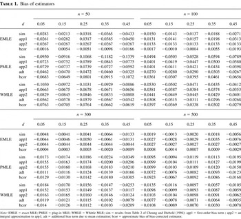
We compute the various approximations presented in the previous section and compare them to the simulated results obtained by Cheung and Diebold (1994). Table 1 contains bias of the three estimators for the ARFIMA(0,d,0) model with n = 50, 100, 300, and 500 and d in the range [0.05, 0.45] at a 0.1 grid. The terms app1 and app2 correspond to the first and second type approximations for each of the estimators, as described in the previous section. The adt terms correspond to the additional bias terms

, for the PMLE and WMLE, respectively. The simulated values of Cheung and Diebold (1994) are taken to be the benchmark. Note that for the Whittle likelihood, Cheung and Diebold (1994, p. 305) considered a minimization of

This term is simply a numerical version of the second term in (5). When σ² = 1, the first term in (5) reduces to a constant.

Bias of estimators

We start with Table 1. In general, all the approximations improve with n, and the approximations of the first type are superior to those of the second type. However, the latter are much simpler to compute, especially for large n. The main feature of the table is that the additional bias term of the PMLE captures much of the difference between the simulated biases of the EMLE and the PMLE. This shows that the additional term is not only nonnegligible but in fact dominant in terms of real magnitude (as opposed to order of magnitude) for the sample sizes under consideration. The simplified bias approximations of all estimators deteriorate as d increases. The reason is that

is the leading term in the approximation of

and although the former is independent of d, the same does not hold for higher order terms in the expansion for

. See Lieberman and Phillips (2004b) for discussion. Both

are based on

, so that the deterioration as d increases affects the bias of these estimators also. As seen from the bcor entries in the table, the reduction in the bias of the bias-corrected estimators can be dramatic.

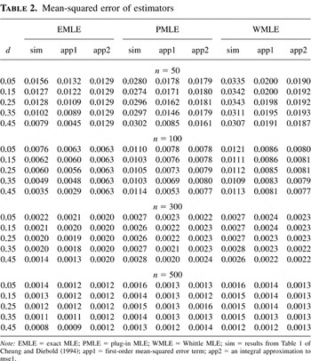
Mean-squared errors are considered in Table 2. It appears that the approximations of the first type are accurate for all estimators and that the approximation errors diminish with n, as expected. The variance approximation

is constant, but the mean-squared errors of the PMLE and the WMLE differ slightly as they involve their nonconstant bias approximations. When n = 500, all approximations are excellent and are practically indistinguishable from the simulated values.

Mean-squared error of estimators

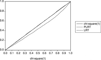
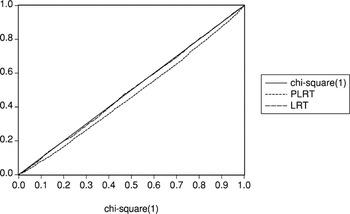
Figures 1 and 2 contain PP plots of the likelihood ratio tests based on the EMLE (LRT) and the PMLE (PLRT) against the asymptotic χ²(1) distribution, with sample sizes of n = 50 and 100. At the 0.01, 0.05, and 0.1 levels of the χ²(1) distribution, the null rejection rates of the ELRT are 0.012, 0.042, 0.096 when n = 50 and 0.01, 0.046, 0.098 when n = 100, respectively. For the PLRT, the values are 0.021, 0.085, 0.154 when n = 50 and 0.016, 0.069, 0.127 when n = 100, respectively. Although the LRT does not seem to need the Bartlett correction for this model and sample sizes, it appears that the curve associated with the PLRT lies markedly underneath the 45° line. It is comforting to know that the first-order distortion in the distribution approximation diminishes when we move from the n = 50 to the n = 100 case. However, the effect of the plugging-in on the χ²(1) approximation to the distribution of the PLRT is substantial and cannot be ignored.

PP plot for the LRT and PLRT in the ARFIMA (0,d,0) model with n = 50 and μ = 0.

PP plot for the LRT and PLRT in the ARFIMA (0,d,0) model with n = 100 and μ = 0.