


1. Introduction
Vortices are coherent fluid entities that can transport properties and mass through an ambient fluid. A number of geometries such as vortex columns, vortex rings and helical vortices have been the focus of specific studies. Given their apparent vulnerability to small fluctuations and susceptibility to disruption, their stability has drawn attentions from scientists and engineers, including the laboratory experiments of Maxworthy (Reference Maxworthy1972, Reference Maxworthy1977), Widnall & Sullivan (Reference Widnall and Sullivan1973) on vortex rings and the theoretical studies of Widnall & Bliss (Reference Widnall and Bliss1971) and Widnall (Reference Widnall1972) on helical vortices. For vortex rings, Widnall, Bliss & Tsai (Reference Widnall, Bliss and Tsai1974) found that a vortex ring is unstable to bending waves (see also Widnall & Tsai Reference Widnall and Tsai1977; Saffman Reference Saffman1978).
We start our discussion with the simplest three-dimensional geometry. A straight vortex column with uniform vorticity inside its core is the simplest geometry in which to study the three-dimensional instabilities of vortices. Infinitesimal disturbances of this basic state of a vortex column are found to be neutrally stable and called Kelvin waves (see Saffman Reference Saffman1992, § 12.1). However, an instability mechanism proposed by Widnall et al. (Reference Widnall, Bliss and Tsai1974) showed the potential for instability: if a vortex column is perturbed by a small parameter,  $\epsilon$, to account for a small geometric or physical effect, the resulting steady-state solution can be written as a perturbation series of
 $\epsilon$. This basic solution is then disturbed by Kelvin waves, which can interact with the
 $O(\epsilon )$ part of the basic state, potentially leading to instabilities. For example, a vortex column subjected to the external strain field
 $(\epsilon y, -\epsilon x,0)$ perpendicular to the axis of the vortex column, is unstable as was discovered by Moore & Saffman (Reference Moore and Saffman1975) and Tsai & Widnall (Reference Tsai and Widnall1976). This is known as the Moore–Saffman–Tsai–Widnall (MSTW) instability. The strained vortex column disturbed by Kelvin waves whose interaction leads to a resonance between two Kelvin waves with azimuthal wavenumber separated by two. This resonance leads to the exponential growth of infinitesimal waves. The MSTW instability has been studied extensively by, for example, Eloy & Le Dizès (Reference Eloy and Le Dizès2001) and Fukumoto (Reference Fukumoto2003), and is related to the elliptic instability in the short-wave limit (see Bayly Reference Bayly1986; Waleffe Reference Waleffe1990; Leweke & Williamson Reference Leweke and Williamson1998).
The same perturbation expansion in  $\epsilon$ can be used for the stability analysis of a thin vortex ring. For a thin vortex ring,
 $\epsilon$ is defined as
 \begin{equation} \epsilon = \frac{a}{R}, \end{equation}
where  $a$ is its core size and
 $R$ is the ring radius. If
 $\epsilon \ll 1$, the ring appears locally as a vortex tube perturbed by small curvature
 $\epsilon$. We obtain the basic state solution for a vortex ring as an expansion in
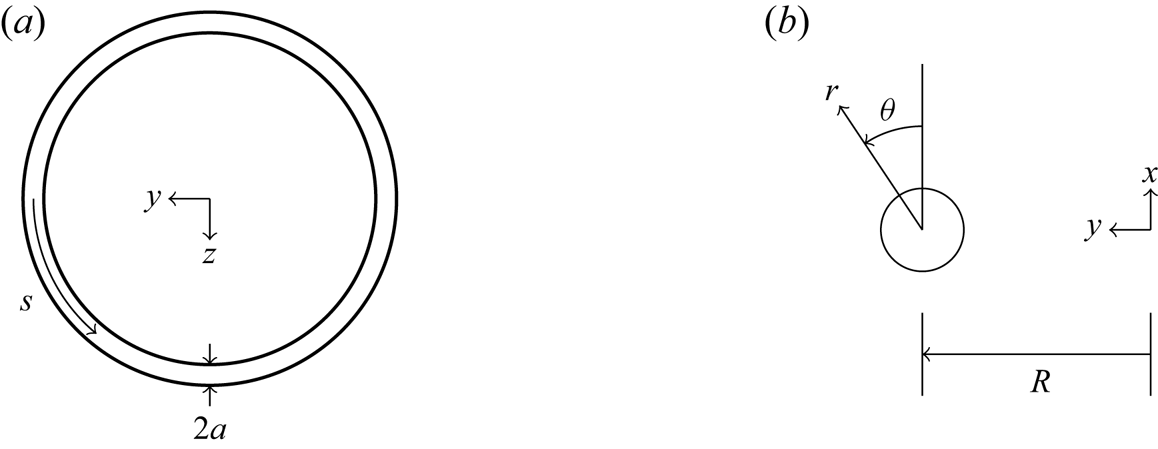
 $\epsilon$. Using the coordinates in figure 1, the resulting instability problem was first set up for a thin vortex ring with an uniform core in Widnall & Tsai (Reference Widnall and Tsai1977). Their short-wavelength analysis shows that the MSTW instability arises from the interaction between Kelvin waves and the basic state at
 $O(\epsilon ^2)$. They concluded that the MSTW instability is responsible for the instability of a thin vortex ring observed in the experiments of Widnall & Sullivan (Reference Widnall and Sullivan1973). However, Hattori & Fukumoto (Reference Hattori and Fukumoto2003) discovered another instability that they named curvature instability. They showed that disturbances are then also unstable in the short-wavelength limit by calculating the growth rate using the geometric optics method. Fukumoto & Hattori (Reference Fukumoto and Hattori2005) then carried out a normal mode analysis using the setup of Widnall & Tsai (Reference Widnall and Tsai1977). A dipole field arising from the basic state in
 $O(\epsilon )$ leads to resonances between two Kelvin waves of wavenumber separated by
 $1$ and instability emerges. All possible resonant pairs of Kelvin waves with azimuthal wavenumber
 $m$ and
 $m+1$ were examined, and larger
 $m$ were found to be more unstable. Fukumoto & Hattori (Reference Fukumoto and Hattori2005) also argued that curvature instability is more unstable than the MSTW instability for a uniform core when
 $\epsilon \ll 1$.
(a) Top view of a thin vortex ring and (b) a cross-section view of the  $xy$-plane. The ring moves in the
 $x$-direction (
 $\theta =0$).

Recent studies have examined vortices with a non-uniform core. Blanco-Rodriguez & Le Dizès (Reference Blanco-Rodriguez and Le Dizès2016, Reference Blanco-Rodriguez and Le Dizès2017) used Gaussian distributions of vorticity for the vortex core and subjected to elliptic and curvature instabilities. Hattori, Blanco-Rodriguez & Le Dizès (Reference Hattori, Blanco-Rodriguez and Le Dizès2019) studied the short-wavelength instabilities of a vortex ring with Gaussian distributions of vorticity and swirl. They found from direct numerical simulations that only the elliptic instability is observed when there is no swirl flow, while the curvature instability emerges when swirl is present but is limited to certain wavenumber range. This is the first numerical evidence confirming the curvature instability of a vortex ring.
All the studies cited previously are for constant-density flows. There are, however, many example of vortex rings in natural and industrial situations for which density effects are important. Vortex rings generated by density differences are examples of thermals (Turner Reference Turner1973), and are important in geological and environmental safety applications. Saffman (Reference Saffman1992, § 5.8) discussed the motion of buoyant vortex rings using conserved quantities, while Baumann, Joseph & Mohr (Reference Baumann, Joseph and Mohr1992) examined their fall. Dolphins are known to create air-filled bubble rings (Marten et al. Reference Marten, Shariff, Psarakos and White1996). Once created, these thin hollow rings seem to survive until the dolphins destroy them, raising the question of their stability. Here we aim to extend the linear stability analysis to a vortex ring with density differing from that of its ambient.
The densities are unequal but constant inside and outside the core. Surface tension is also considered. This configuration is consistent with previous work, and we follow them by taking a Rankine vortex as the ring's core. In part 1 of the present work, we follow the calculation in Fukumoto & Hattori (Reference Fukumoto and Hattori2005) and carry out a normal mode analysis for the curvature instability. In § 2, the linearised governing equations and boundary conditions for infinitesimal disturbances are given. The basic state solution as a perturbation series up to  $O(\epsilon )$ is also given. We discuss Kelvin waves with densities and surface tension in § 3. The growth rate and the half-bandwidth of the curvature instability and numerical examples are presented in § 4. We draw conclusions in § 5, while some technical results are presented in the appendices and a symbolic computer algebra code is available as supplementary material available at https://doi.org/10.1017/jfm.2020.845. We return to the MSTW instability in Part 2 (Chang & Llewellyn Smith Reference Chang and Llewellyn Smith2021).
2. Formulation
A vortex ring with radius  $R$ and core size
 $a$ is considered. The core is taken to be thin, so that
 $\epsilon =a/R \ll 1$. The outer region and the vortical core have constant densities
 $\rho _1$ and
 $\rho _2$ respectively. The circulation around the core is
 $\varGamma$. The problem is non-dimensionalised using length scale
 $a$, velocity scale
 $U_c=\varGamma /(2 {\rm \pi}a)$ and time scale
 $2{\rm \pi} a^2/\varGamma$, while the pressure scale is taken to be
 $\rho _2 (\varGamma /2{\rm \pi} a)^2$. The velocity potential describing the outer irrotational flow is scaled by
 $\varGamma /2 {\rm \pi}$.
Density differences in the presence of a gravity field lead to buoyancy effects acting on the vortex ring. However, buoyant vortex rings (whether light or heavy,  $\rho _1\ne \rho _2$) do not move steadily (see e.g. Turner Reference Turner1957; Pedley Reference Pedley1968; Chang & Llewellyn Smith Reference Chang and Llewellyn Smith2018). Light vortex rings expand with the radius growing like
 $\sqrt {t}$, and the speed slows down as
 $t^{-1/2}\ln t$. To avoid this complication, we consider buoyancy to have a slowly-varying effect so that the mean flow is ‘frozen’ in time. This is justified on the basis that the Froude number
 \begin{equation} Fr = \frac{\varGamma/(2{\rm \pi} a)}{\sqrt{ag}} \end{equation}
is very large. The time scale of the rotational motion inside the core  $\sim a^2/\varGamma$, while the time scale of buoyant motion is
 $\sim \sqrt {a/g}$. Then
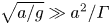 $\sqrt {a/g}\gg a^2/\varGamma$ is equivalent to
 $Fr \gg 1$, so the vortex ring can be considered frozen on the time scale of
 $a^2/\varGamma$. Therefore, the gravity term is omitted in the governing equations.
2.1. Governing equations
Following Fukumoto & Hattori (Reference Fukumoto and Hattori2005), we use a coordinate system  $(r, \theta , s)$ co-moving with the ring, as shown in figure 1, with velocity
 $\boldsymbol {u}=(u,v,w)$. The undisturbed core boundary is taken to be
 $r = 1$. Since the core is rotational, the governing equations in the inner region are the Euler equations,
 \begin{equation} \boldsymbol{\nabla} \boldsymbol{\cdot} \boldsymbol{u} = 0, \quad \frac{\partial \boldsymbol{u}}{\partial t} + \boldsymbol{u} \boldsymbol{\cdot} \boldsymbol{\nabla} \boldsymbol{u} = - \boldsymbol{\nabla} p. \end{equation}
Vorticity is zero outside the core of the vortex ring, and the Laplace equation in the outer irrotational region is
 \begin{equation} \nabla^2 \varPhi = 0, \end{equation}
where  $\varPhi$ is the velocity potential.
In the  $(r, \theta , s)$ coordinates, the Euler equations become
 \begin{gather} \frac{\partial u}{\partial t} +\boldsymbol{u} \boldsymbol{\cdot} \boldsymbol{\nabla} u-\frac{v^2}{r} -\epsilon\frac{w^2 \sin \theta}{h_s} = -\frac{\partial p}{\partial r}, \end{gather}
 \begin{gather}\frac{\partial v}{\partial t} +\boldsymbol{u} \boldsymbol{\cdot} \boldsymbol{\nabla} v+\frac{uv}{r} -\epsilon\frac{w^2 \cos \theta}{h_s} = -\frac{1}{r}\frac{\partial p}{\partial \theta}, \end{gather}
 \begin{gather}\frac{\partial w}{\partial t} +\boldsymbol{u} \boldsymbol{\cdot} \boldsymbol{\nabla} w+\epsilon\frac{w(u \sin \theta+v \cos \theta)}{h_s} = -\frac{1}{h_s}\frac{\partial p}{\partial s}, \end{gather}
where  $h_s = 1+\epsilon r \sin \theta$, and
 \begin{equation} \boldsymbol{u} \boldsymbol{\cdot} \boldsymbol{\nabla} = u\frac{\partial}{\partial r} +\frac{v}{r}\frac{\partial}{\partial \theta}+\frac{w}{h_s}\frac{\partial}{\partial s}. \end{equation}
The continuity equation is
 \begin{equation} \frac{1}{r}\frac{\partial}{\partial r}(ru) +\frac{1}{r}\frac{\partial v}{\partial \theta}+\frac{1}{h_s}\frac{\partial w}{\partial s}+\frac{\epsilon}{h_s} (u \sin \theta+v \cos \theta) = 0. \end{equation}
Outside the core, Laplace's equation becomes
 \begin{equation} \frac{1}{r}\frac{\partial}{\partial r}\left(r\frac{\partial \varPhi}{\partial r}\right) +\frac{1}{r^2}\frac{\partial^2 \varPhi}{\partial \theta^2}+\frac{1}{h_s^2}\frac{\partial^2 \varPhi}{\partial s^2}+\frac{\epsilon}{h_s} \left(\sin \theta\frac{\partial \varPhi}{\partial r}+\frac{\cos \theta}{r}\frac{\partial \varPhi}{\partial \theta}\right) = 0. \end{equation}
2.2. Boundary conditions
The boundary of the vortex is taken to be  $r=F(\theta \; \epsilon)$, where
 $F(\theta \; \epsilon )$ will be found as part of the solution. The inner and outer solutions are matched on the core boundary. For inviscid flows, the matching conditions are given by the kinematic and the dynamic conditions. The kinematic condition is
 \begin{equation} \left. \frac{\mathrm{D} }{\mathrm{D} t}(r-F) \right |_{r\to F^-} = \left. \frac{\mathrm{D} }{\mathrm{D} t}(r-F) \right |_{r\to F^+} = 0, \end{equation}
where  $\mathrm {D}/\mathrm {D} t$ is the usual Lagrangian time derivative and
 $\pm$ represent the inside and outside of the boundary, respectively.
The dynamic condition relates the jump in pressure across the boundary to surface tension. Because the outer flow is irrotational, we can use the unsteady Bernoulli equation to express the pressure there in terms of a velocity potential. Taking pressure to vanish at infinity without loss of generality, one obtains
 \begin{equation} \frac{\rho_2}{\rho_1} p + \frac{\partial \varPhi}{\partial t} + {\frac{1}{2}} |\boldsymbol{\nabla} \varPhi|^2 = S \boldsymbol{\nabla} \boldsymbol{\cdot} \boldsymbol{n}. \end{equation}
Here  $S$ is dimensionless surface tension
 $\sigma /[\rho _1 a(\varGamma /2{\rm \pi} a)^2]$ and
 $\boldsymbol {n}=\boldsymbol {\nabla } (r-F)/|\boldsymbol {\nabla } (r-F)|$ is the outward normal vector on the boundary.
2.3. The mean flow solution
Linear stability analysis needs a steady-state solution as a base to be ‘perturbed’ by infinitesimal disturbances. At  $O(1)$, a steady-state solution exists describing the vortex ring in a moving coordinate system. The solution (written using uppercase letters) can be obtained as a perturbation series in
 $\epsilon$:
 \begin{equation} \boldsymbol{U} = \boldsymbol{U}_0 +\epsilon \boldsymbol{U}_1+\cdots, \quad P = P_0 +\epsilon P_1+\cdots, \quad \varPhi = \varPhi_0 +\epsilon \varPhi_1+\cdots, \end{equation}
as in § 2 of Fukumoto & Hattori (Reference Fukumoto and Hattori2005) who take  $\rho _1=\rho _2$. The leading-order solution corresponds to a vortex column perturbed by the small dimensionless curvature of the vortical core. The shape of the boundary is formally expanded in
 $\epsilon$, but is taken to be circular, so that the expansion is redundant.
Here we use the same basic state with a correction for  $\rho _1\ne \rho _2$. A normal mode analysis of the disturbances then leads to a dispersion relation and possible instability. We now obtain the basic solution for the stability calculation using (2.12a–c). The leading-order mean flow solution is the Rankine vortex with velocity and pressure fields
 \begin{equation} (U_0, V_0, W_0) = (0, r, 0), \quad P_0 = \frac{1}{2}\left(r^2-1-\frac{\rho_1}{\rho_2}\right) +\frac{\rho_1}{\rho_2}S \end{equation}
inside the core ( $r<1$). The boundary of the vortex is circular, so that
 $F_0=1$. The velocity potential outside (
 $r>1$) is
 \begin{equation} \varPhi_0 = \theta. \end{equation}
Curvature leads to the following  $O(\epsilon )$ contribution to the mean flow:
 \begin{equation} U_1 = \tfrac{5}{8}(1-r^2) \cos{\theta}, \quad V_1 = \tfrac{1}{8}(7r^2-5) \sin{\theta}, \quad P_1 = \left(\tfrac{3}{8}r^3-\tfrac{5}{8}r \right) \sin{\theta} \end{equation}
in the inner region, while the outer solution is a dipole field:
 \begin{equation} \varPhi_1 = \frac{1}{8}\left[ 2\left(r-\frac{1}{r}\right) -\frac{\rho_2}{\rho_1}\left(r+\frac{1}{r}\right) -4S\left(r+\frac{1}{r}\right) -4r \log r \right] \cos \theta. \end{equation}
The shape of the boundary has been taken to remain circular to  $O(\epsilon )$, that is,
 $F_1=0$. See appendix A for detailed calculations yielding (2.13a,b)–(2.16). The mean flow solution can be compared with the result of Fukumoto & Hattori (Reference Fukumoto and Hattori2005) by taking
 $\rho _2/\rho _1=1$ and
 $S=0$.
2.4. Linearised equations and boundary conditions for infinitesimal disturbances
We disturb the mean flow derived in the previous subsection, and write
 \begin{equation} U+\tilde{u}, \quad V+\tilde{v}, \quad W+\tilde{w}, \quad P+\tilde{p}, \quad \varPhi+\tilde{\phi}, \end{equation}
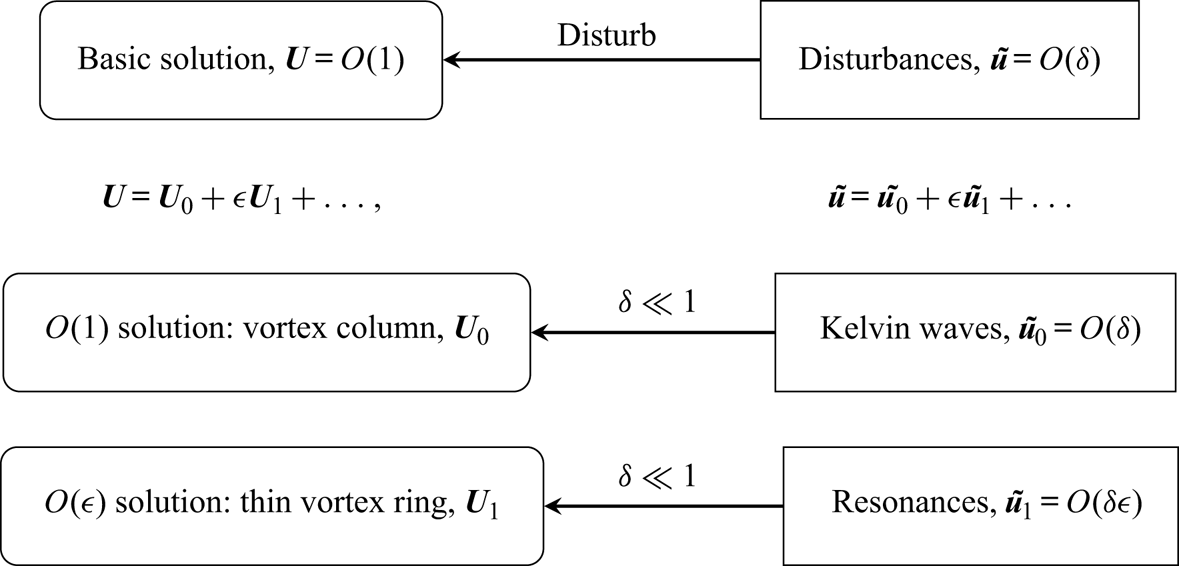
where the disturbed boundary is  $r=F+\tilde {f}$. The structure of the solution is outlined in figure 2. Disturbances, denoted by tilde, are
 $O(\delta )$ compared with the mean flow with
 $\delta \ll 1$. In parallel, the solution is expanded in
 $\epsilon$, the small non-dimensional core size. For this stability analysis, we are interested in disturbances at
 $O(\delta )$ and
 $O(\delta \epsilon )$. The vortex column solution given by
 $\boldsymbol {U}_0$ is neutrally stable, supporting Kelvin waves
 $\tilde {\boldsymbol {u}}_0$. However, when a small parameter
 $\epsilon$ is introduced, instability can be excited corresponding to resonance or parametric instability. Disturbances are decomposed into normal modes in
 $s$ and
 $t$, that are expanded in
 $\epsilon$ as
 \begin{gather} \tilde{\boldsymbol{u}} = \left(\tilde{\boldsymbol{u}}_0 +\epsilon\tilde{\boldsymbol{u}}_1 +\cdots\right) \mathrm{e}^{\mathrm{i}(ks-\omega t)}, \end{gather}
 \begin{gather}\tilde{p} = \left(\tilde{p}_0 +\epsilon \tilde{p}_1 +\cdots\right) \mathrm{e}^{\mathrm{i}(ks-\omega t)}, \end{gather}
 \begin{gather}\tilde{\phi} = (\tilde{\phi}_0 +\epsilon\tilde{\phi}_1 +\cdots)\,\mathrm{e}^{\mathrm{i}(ks-\omega t)}, \end{gather}
where the real part is implicit with no loss of generality. The wavenumber and the frequency are also expanded as
 \begin{equation} k = k_0 +\epsilon k_1 +\cdots, \quad \omega = \omega_0 +\epsilon\omega_1 +\cdots. \end{equation}
The core boundary disturbance is
 \begin{equation} \tilde{f} = (\,\tilde{f}_0 +\epsilon \tilde{f}_1 + \cdots)\,\mathrm{e}^{\mathrm{i}(ks-\omega t)}. \end{equation}
As the disturbances  $(\tilde {\boldsymbol {u}}, \tilde {p}, \tilde {\phi })$ are small compared with the basic solution
 $(\boldsymbol {U}, P, \varPhi )$, (2.6)–(2.9) can be linearised.
Schematic structure of the present calculation.

2.4.1.  $O(\delta )$ linearised equations and boundary conditions

The linearised equations for disturbances at  $O(\delta )$ are
 \begin{gather} -\mathrm{i} \omega_0 \tilde{u}_0 +\frac{V_0}{r}\frac{\partial \tilde{u}_0}{\partial \theta} -\frac{2 V_0 \tilde{v}_0}{r} = -\frac{\partial \tilde{p}_0}{\partial r}, \end{gather}
 \begin{gather}-\mathrm{i} \omega_0 \tilde{v}_0 +\frac{V_0}{r}\frac{\partial \tilde{v}_0}{\partial \theta} + \left( \frac{\partial V_0}{\partial r} + \frac{V_0}{r} \right) \tilde{u}_0 = -\frac{1}{r}\frac{\partial \tilde{p}_0}{\partial \theta}, \end{gather}
 \begin{gather}-\mathrm{i} \omega_0 \tilde{w}_0 +\frac{V_0}{r}\frac{\partial \tilde{w}_0}{\partial \theta} = -\frac{\partial \tilde{p}_0}{\partial s}, \end{gather}
 \begin{gather}\frac{1}{r}\frac{\partial}{\partial r}(r \tilde{u}_0) +\frac{1}{r}\frac{\partial \tilde{v}_0}{\partial \theta}+\frac{\partial \tilde{w}_0}{\partial s} =0 \end{gather}
inside and
 \begin{equation} \frac{1}{r}\frac{\partial}{\partial r}\left(r \frac{\partial \tilde{\phi}_0}{\partial r}\right) +\frac{1}{r^2}\frac{\partial^2 \tilde{\phi}_0}{\partial \theta^2}+\frac{\partial^2 \tilde{\phi}_0}{\partial s^2}=0 \end{equation}
outside the core. The linearised boundary conditions at  $r=1$ are
 \begin{gather} \tilde{u}_0 = \frac{\partial \tilde{\phi}_0}{\partial r} = -\mathrm{i} \omega_0\,\tilde{f}_0 +\frac{\partial \tilde{f}_0}{\partial \theta}, \end{gather}
 \begin{gather}\frac{\rho_2}{\rho_1} \tilde{p}_0 -\mathrm{i}\omega_0\tilde{\phi}_0 +\frac{\partial \tilde{\phi}_0}{\partial \theta} = \left(1-\frac{\rho_2}{\rho_1} \right) \tilde{f}_0 -S \left(\frac{\partial^2 \tilde{f}_0}{\partial \theta^2} -k_0^2\,\tilde{f}_0 \right). \end{gather}
The solutions to this problem are Kelvin waves, as detailed in the following and in appendix B.
2.4.2. $O(\delta \epsilon )$ linearised equations and boundary conditions

We proceed to  $O(\delta \epsilon )$. The inner solution satisfies
 \begin{align} -\mathrm{i} \omega_0 \tilde{u}_1+\frac{\partial \tilde{u}_1}{\partial \theta} -2\tilde{v}_1+\frac{\partial \tilde{p}_1}{\partial r} &= \left( \mathrm{i} \omega_1-\frac{\partial U_1}{\partial r}\right)\tilde{u}_0 -U_1\frac{\partial \tilde{u}_0}{\partial r}-\frac{V_1}{r}\frac{\partial \tilde{u}_0}{\partial \theta} \nonumber\\ &\quad-\left(\frac{1}{r}\frac{\partial U_1}{\partial \theta}-\frac{2V_1}{r}\right) \tilde{v}_0, \end{align}
 \begin{align} -\mathrm{i} \omega_0 \tilde{v}_1 +2\tilde{u}_1+\frac{\partial \tilde{v}_1}{\partial \theta}+\frac{1}{r}\frac{\partial \tilde{p}_1}{\partial \theta} &= \left( \mathrm{i} \omega_1-\frac{1}{r}\frac{\partial V_1}{\partial \theta}-\frac{V_1}{r}\right)\tilde{v}_0 -U_1\frac{\partial \tilde{v}_0}{\partial r}-\frac{V_1}{r}\frac{\partial \tilde{v}_0}{\partial \theta} \nonumber\\ &\quad-\left(\frac{\partial V_1}{\partial r}+\frac{V_1}{r}\right) \tilde{u}_0, \end{align}
 \begin{align}-\mathrm{i} \omega_0 \tilde{w}_1+\frac{\partial \tilde{w}_1}{\partial \theta} +\mathrm{i} k_0 \tilde{p}_1 &= -\mathrm{i} (k_1 -k_0 r\sin \theta) \tilde{p}_0 +(\mathrm{i} \omega_1-r\cos \theta)\tilde{w}_0\nonumber\\ &\quad-U_1\frac{\partial \tilde{w}_0}{\partial r}-\frac{V_1}{r}\frac{\partial \tilde{w}_0}{\partial \theta}, \end{align}
 \begin{gather}\frac{\partial \tilde{u}_1}{\partial r} +\frac{\tilde{u}_1}{r} +\frac{1}{r}\frac{\partial \tilde{v}_1}{\partial \theta}+\mathrm{i} k_0 \tilde{w}_1 = -\mathrm{i} (k_1-k_0 r\sin \theta) \tilde{w}_0 -\tilde{u}_0 \sin \theta -\tilde{v}_0\cos \theta. \end{gather}
The velocity potential outside satisfies
 \begin{align} \frac{\partial^2 \tilde{\phi}_1}{\partial r^2}+\frac{1}{r}\frac{\partial \tilde{\phi}_1}{\partial r} +\frac{1}{r^2}\frac{\partial^2 \tilde{\phi}_1}{\partial \theta^2} -k_0^2 \tilde{\phi}_1 = 2(k_0 k_1 -k_0^2r\sin \theta) \tilde{\phi}_0 -\sin \theta \frac{\partial \tilde{\phi}_0}{\partial r} -\frac{\cos \theta}{r} \frac{\partial \tilde{\phi}_0}{\partial \theta}. \end{align}
The linearised boundary conditions at  $r=1$ are
 \begin{gather} -\mathrm{i} \omega_0\,\tilde{f}_1 +\frac{\partial \tilde{f}_1}{\partial \theta} -\tilde{u}_1 = \mathrm{i}\omega_1\,\tilde{f}_0 -V_1\frac{\partial \tilde{f}_0}{\partial \theta} +\frac{\partial U_1}{\partial r}\tilde{f}_0, \end{gather}
 \begin{gather}\tilde{u}_1 = \frac{\partial \tilde{\phi}_1}{\partial r}, \end{gather}
 \begin{align} \frac{\rho_2}{\rho_1} \tilde{p}_1 &-\mathrm{i}\omega_0\tilde{\phi}_1 +\frac{\partial \tilde{\phi}_1}{\partial \theta} = \mathrm{i} \omega_1\tilde{\phi}_0 -\frac{\partial \varPhi_1}{\partial \theta} \frac{\partial \tilde{\phi}_0}{\partial \theta} +\left(1-\frac{\rho_2}{\rho_1} \right) \tilde{f}_1 +2S\sin \theta \tilde{f}_0 \nonumber\\ &\quad -S \left(\frac{\partial^2 \tilde{f}_1}{\partial \theta^2}-k_0^2\, \tilde{f}_1 -2k_0 k_1\, \tilde{f}_0 +2\sin\theta ~k_0^2 \,\tilde{f}_0 +\cos \theta\frac{\partial \tilde{f}_0}{\partial \theta} \right). \end{align}
The dispersion relations at  $O(\delta )$ and
 $O(\delta \epsilon )$ are obtained from ((2.28)–(2.29)), and ((2.36)–(2.37)) respectively. The condition (2.35) is used only to determine the boundary shape
 $\tilde {f}_1$, and is not required to calculate the dispersion relation when surface tension term vanishes (Fukumoto & Hattori Reference Fukumoto and Hattori2005).
3. $O(\delta )$ solution: Kelvin waves on a vortex column

The disturbances satisfying (2.23)–(2.27) are written as
 \begin{equation} \tilde{\boldsymbol{u}}_0(r,\theta) = \boldsymbol{u}_0^{(m)}(r) \mathrm{e}^{\mathrm{i} m\theta}, \quad \tilde{p}_0(r,\theta) = p_0^{(m)}(r) \mathrm{e}^{\mathrm{i} m\theta}, \quad \tilde{\phi}_0(r,\theta) = \phi_0^{(m)}(r) \mathrm{e}^{\mathrm{i} m\theta}, \end{equation}
where  $m$ is the azimuthal wavenumber. The solution at leading order is a Kelvin wave, described in appendix B. The Kelvin waves are coupled to the dipole field (2.15a–c)–(2.16) through the right-hand sides of (2.30)–(2.34). When two Kelvin waves with wavenumber
 $m$ and
 $m+1$ appear in the forcing terms on the right-hand side of (2.30)–(2.34), the solution at the
 $O(\delta \epsilon )$ will possess modes for
 $m-1$,
 $m$,
 $m+1$ and
 $m+2$. We focus on the resonance between pairs of Kelvin waves
 $(m,m+1)$ in this paper.
The solution (B 1) and (B 3) contains the amplitudes of Kelvin waves,  $\alpha _0$,
 $\beta _0$, that are determined using the boundary conditions. The boundary conditions (2.28) and (2.29) for wavenumber
 $m$ become
 \begin{gather} -\mathrm{i}(\omega_0-m) f_0^{(m)} = u_0^{(m)} = \frac{\mathrm{d} \phi_0}{\mathrm{d} r}^{(m)}, \end{gather}
 \begin{gather}\frac{\rho_2}{\rho_1} p_0^{(m)} -\mathrm{i} (\omega_0 -m) \phi_0^{(m)} =\left(1-\frac{\rho_2}{\rho_1} \right) f_0^{(m)} +S (m^2+k_0^2) f_0^{(m)}. \end{gather}
Substituting  $p_0^{(m)}$,
 $u_0^{(m)}$,
 $\phi _0^{(m)}$ and
 $f_0^{(m)}$ (see appendix B) into the previous equations, we obtain a set of homogeneous linear equations for
 $\alpha _0^{(m)}$ and
 $\beta _0^{(m)}$. For non-trivial
 $\alpha _0^{(m)}$ and
 $\beta _0^{(m)}$, the determinant must be zero, which gives the dispersion relation for mode
 $m$:
 \begin{align} &\left[ 1 +\frac{E_{1}}{(\omega_{0}-m)^2} \left(m -k_{0} \frac{\textrm{K}_{m+1}(k_{0})}{\textrm{K}_{m}(k_{0})}\right) \right] \textrm{J}_{m+1}(\eta_{1}) = \left\{ -m\frac{\omega_{0}-m}{\omega_{0}-m+2} \right. \notag\\ &\quad +\left. \left[\frac{\rho_{2}}{\rho_{1}}-E_{1} \frac{m}{(\omega_{0}-m)(\omega_{0}-m+2)}\right] \left(m -k_{0} \frac{\textrm{K}_{m+1}(k_{0})}{\textrm{K}_{m}(k_{0})}\right) \right\} \frac{\eta_{1}}{k_{0}^{2}} \textrm{J}_{m}(\eta_{1}), \end{align}
where
 \begin{equation} E_1 = 1-\frac{\rho_2}{\rho_1} +S(k_0^2+m^2). \end{equation}
Here  $\textrm{J}_m$ is the Bessel function of the first kind and
 $\textrm{K}_m$ is the modified Bessel function of the second kind;
 $\eta _1$ is the radial wavenumber for the Kelvin wave defined in (B 2). For the
 $m+1$ wave, the boundary conditions are the same formulae as in (3.3) except that
 $m$ is replaced by
 $m+1$, and similarly for the solution in appendix B. Using the boundary conditions and the solution for the
 $m+1$-mode, we obtain the dispersion relation,
 \begin{align}
&\left[ 1 - \frac{E_2}{(\omega_0-m-1)^2} \left(m+1 +k_0
\frac{\textrm{K}_{m}(k_0)}{\textrm{K}_{m+1}(k_0)}\right) \right]
\textrm{J}_{m}(\eta_2) =
\left\{-(m+1)\frac{\omega_0-m-1}{\omega_0-m-3} \right.
\nonumber\\ &\quad +\left.\left[\frac{\rho_2}{\rho_1}+E_2
\frac{m+1}{(\omega_0-m-1)(\omega_0-m-3)}\right] \left(m+1
+k_0 \frac{\textrm{K}_{m}(k_0)}{\textrm{K}_{m+1}(k_0)}\right) \right\}
\frac{\eta_2}{k_0^2}~\textrm{J}_{m+1}(\eta_2),
\end{align}
for it, where  $E_2 = 1-\rho _2/\rho _1 +S[k_0^2+(m+1)^2]$ and
 $\eta _2$ is also the radial wavenumber for
 $m+1$.
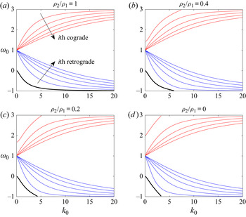
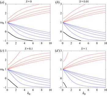
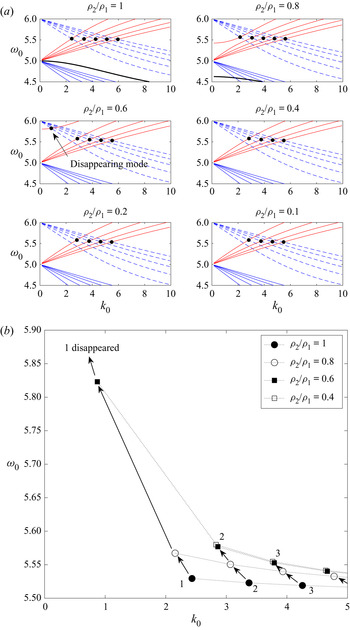
If we set the density ratio to one and surface tension to zero, we can easily recover (3.6) and (3.4) from the dispersion relation for Kelvin waves ((B 6) and (B 7) in Fukumoto & Hattori Reference Fukumoto and Hattori2005). The dispersion curves for modes for  $m=1$ are plotted in figures 3 and 4 as functions of density ratio and surface tension. There are infinitely many branches of cograde and retrograde modes for each Kelvin wave with wavenumber
 $m$. Figures 3 and 4 show the first five branches in each of the cograde and the retrograde modes. An isolated branch is also shown. We designate the branch with the largest value of
 $|\omega _0-m|$ for a given
 $k_0$ as the first cograde/retrograde branch and then counting the branches toward
 $\omega _0=m$. Thus, the uppermost cograde branch and the bottommost retrograde branch are the first cograde and first retrograde modes. Every mode of
 $m$ has cograde branches going upward where
 $\omega _0>m$ and retrograde branches going downward where
 $\omega _0 < m$, plotted in red and blue, respectively. All the cograde and retrograde branches radiate out from
 $(k_0,\omega _0)=(0,m)$ when
 $\rho _2/\rho _1=1$. There is an isolated branch starting from
 $(0,m-1)$ that only appears when
 $m\ne 0$. In figure 3, we can see how decreasing the density ratio from one to zero changes the dispersion relation of Kelvin waves: all the branches move away from the centreline
 $\omega _0=m$, the cograde branches shift toward
 $\omega _0=m+2$ and the retrograde and isolated branches shift toward
 $\omega _0=m-2$. While the branches shift, the starting point of all the branches remains the same. One exception is the outermost cograde branch: its starting point moves from
 $(0,m)$ upward to
 $(0,m+1)$ when
 $\rho _2/\rho _1$ drops to zero in figure 3. We refer this as ‘isolation’ of the cograde mode. Similar changes are also observed when surface tension increases from zero to one in figure 4: the cograde branches move toward
 $\omega _0=m+2$, the retrograde and isolated branches move toward
 $\omega _0=m-2$. The uppermost cograde mode departs from the other cograde modes and becomes isolated. The effect of this change is that a intersection point could disappear when
 $(\rho _2/\rho _1,S)$ deviates from
 $(1,0)$ (see figure 5).
Dispersion curves for the Kelvin wave with  $m=1$ for density ratios from one to zero. Red curves are cograde branches and blue curves are retrograde branches. Only the first five branches are plotted, which have the largest value of
 $|\omega _0-m|$ in each of the cograde and retrograde modes. An isolated branch (thick black curve) can be seen emanating from
 $(k_0,\omega _0)=(0,m-1)$. Surface tension is zero for all plots.

Dispersion curves for the Kelvin wave with  $m=1$ as surface tension increases from zero to one. The density ratio is fixed at
 $\rho _2/\rho _1=0.4$; other ratios give qualitatively similar results.

(a) Dispersion curves for a pair of Kelvin waves  $m=(5,6)$ for density ratio varying from one to zero; surface tension is zero. Solid curves are for
 $m=5$ and dotted curves for
 $m=6$; red is for cograde branches, blue is for retrograde branches and the black thick curve is the isolated branch. The black dots represent the first five principal modes. One of the back dots disappears when
 $\rho _2/\rho _1$ drops to
 $0.4$ or less. (b) The migration of the principal modes as density ratio decreases. There is no mode ‘1’ when
 $\rho _2/\rho _1=0.4$.

There is another significant change to the Kelvin waves with density and surface tension: the top branches and the bottom downward branches, that is, the first cograde mode and the isolated mode, respectively, have a real part  $\omega _0$ that disappears at some point
 $(k_0, m\pm 2)$ on the top or the bottom edge of the plot. Since
 $k_0$ is always real, the radial wavenumber
 $\eta _1 = k_0\sqrt {4/(\omega _0-m)^2-1}$ is real only if
 $\omega _0 \in (m-2, m+2)$. For the case of
 $\rho _2/\rho _1=1$ and
 $S=0$, all the branches lie between
 $\omega _0=m-2$ and
 $m+2$, so the Kelvin waves are always neutrally stable. When
 $\rho _2/\rho _1<1$ and
 $S\ne 0$, the isolated branch reaches
 $\omega _0=m-2$ on the edge of the plot, for example at
 $k_0=4.2$ in the plot for
 $S=0.01$ of figure 4. The uppermost cograde branch reaches
 $\omega _0=m+2$ at
 $k_0 \approx 5.2$. For
 $|\omega _0-m|>2$, the radial wavenumber
 $\eta _1$ becomes pure imaginary. We can replace it by
 $\mathrm {i} \lambda _1$ where
 $\lambda _1$ is real, then replace the Bessel function of the first kind
 $\textrm{J}_m$ in (3.4) by
 $\mathrm {i}^m I_m(\lambda _1)$. The new dispersion relation is real for
 $|\omega _0-m|>2$, and the upward cograde branch and the downward isolated branch extend beyond
 $\omega _0=m\pm 2$.
When two Kelvin waves for wavenumber differing by  $1$ resonate, all their branches result in infinitely many intersection points when they cross through each other. As mentioned in Fukumoto & Hattori (Reference Fukumoto and Hattori2005), only the intersection points between the cograde modes
 $m$ and the retrograde modes
 $m+1$ are candidates for curvature instability; see figure 5(a) for an example. For the convenience of discussion, we follow Fukumoto & Hattori (Reference Fukumoto and Hattori2005) to define ‘principal modes’. The
 $i$th principal mode is referred to as the intersection point of
 $i$th cograde and
 $i$th retrograde modes, and we indicate the first five principal modes by black dots in figure 5. Their growth rates are larger than those of other intersection points when
 $\rho _2/\rho _1=1$ and
 $S=0$, so they will be the focus of our curvature instability calculations. Although we will show later that they do not always dominate over other intersection points when
 $\rho _2/\rho _1\ne 1$ or
 $S\ne 0$ (see § 4.4). The reader should be aware of that only four dots are shown for
 $\rho _2/\rho _1=0.4$ or below. This is due to the ‘isolation’ of the first cograde branch of
 $m$ as discussed earlier. As it is moving away from the other cograde branches, it no longer crosses the first retrograde branch of
 $m+1$. The first principal mode then disappears. The migration of first few principal modes and the disappearance of the first mode are demonstrated in figure 5(b).
Note that the ‘principal modes’ refer here to the set of principal modes when  $\rho _2/\rho _1=1$ and
 $S=0$. If we choose an arbitrary value of density ratio and plot its dispersion curve, we will obtain a plot like that for
 $\rho _2/\rho _1=0.4$ in figure 5. By looking at that single plot, we would not be able to see that a process of isolation had taken place, and another sequence of intersection points (just below the back dots) would have been taken as principal modes by definition. Since our goal is to investigate the effects of density and surface tension, we to keep track of the same sequence of intersection points, the principal modes for
 $\rho _2/\rho _1=1$ and
 $S=0$.
4. $O(\delta \epsilon )$ solution: curvature as a small perturbation

The solution of the  $O(\delta \epsilon )$ disturbances governed by (2.30)–(2.34) is given in appendix C of Fukumoto & Hattori (Reference Fukumoto and Hattori2005). We do not reproduce it here, given its complexity. The solution contains undetermined coefficients (wave amplitudes)
 $\alpha _1$,
 $\beta _1$, which must be non-zero. The boundary conditions in (2.36) and (2.37) are used to obtain the dispersion relation. Note that in order to include surface tension, we need to compute
 $\tilde {f}_1$ from (2.35) before using the second and the third equations for the dispersion relation. In Fukumoto & Hattori (Reference Fukumoto and Hattori2005),
 $\tilde {f}_1$ is not necessary since surface tension is omitted.
The result of substituting the  $O(\delta \epsilon )$ solutions for modes
 $m$ and
 $m+1$ into (2.36) and (2.37) and the
 $O(\delta \epsilon )$ boundary disturbance
 $\tilde {f}_1$ for the two modes is given in appendix C. Using these results and requiring the coefficients
 $\alpha _1$,
 $\beta _1$ not to vanish leads to the dispersion relation for
 $k_1$ and
 $\omega _1$. The detailed calculation is outlined in appendix C. The dispersion relation takes the form given in (C 14). Given the cumbersome algebra, which is impractical to carry out manually, we use computer-aided symbolic algebra. We validate the result obtained from symbolic algebra with the formulae for the maximum growth rate
 $\sigma _{1max}$ and the instability half-bandwidth
 $\Delta k_1$ given in (2.23) and (2.24) of Fukumoto & Hattori (Reference Fukumoto and Hattori2005). Unfortunately, the two new parameters,
 $\rho _2/\rho _1$ and
 $S$, lead to too much complexity to check the formulae algebraically. Hence, we compare our results with those of Fukumoto & Hattori (Reference Fukumoto and Hattori2005) for specific values. Using the formulae returned by the symbolic algebra, we calculate
 $\sigma _{1max}$ and
 $\Delta k_1$ for given values of
 $m$ and
 $(k_0,\omega _0)$. Then we set
 $\rho _2/\rho _1=1$ and
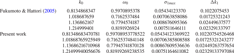
 $S=0$ and compared the numbers with those from Fukumoto & Hattori (Reference Fukumoto and Hattori2005), as listed in table 1 for
 $m=0$ and table 2 for
 $m=5$. Each row in the tables represents a mode of resonance between a
 $(m,m+1)$ pair, while the first row corresponds to the first principal mode. The results agree very well with Fukumoto & Hattori (Reference Fukumoto and Hattori2005) for each of wavenumber
 $m$ and principal modes.
For the  $m=0$ and
 $1$ resonances, present results for
 $\rho _2/\rho _1=1$ compared with table 1 of Fukumoto & Hattori (Reference Fukumoto and Hattori2005).

For the  $m=5$ and
 $6$ resonances, present results for
 $\rho _2/\rho _1=1$ compared with table 2 of Fukumoto & Hattori (Reference Fukumoto and Hattori2005).

4.1. Effect of density variations
In this section, we set surface tension to  $0$ and focus on the effect of density differences.
4.1.1. Heavy core: $\rho _2/\rho _1>1$

We first examine  $\rho _2/\rho _1>1$. In this case, the vortex ring core is denser than the fluid surrounding it (for instance Rayleigh–Taylor instability could create vortex rings when heavier fluid falls through a lighter fluid and rolls up; see, e.g., Baker, Meiron & Orszag Reference Baker, Meiron and Orszag1980; Joly, Fontane & Chassaing Reference Joly, Fontane and Chassaing2005). The first five principal modes for the resonance between
 $(0,1)$ and
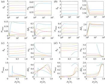
 $(5,6)$ are shown in figures 6(a) and 6(b) respectively. For the
 $(0,1)$ resonance pair, the first principal mode (blue) is most unstable. The growth rates of all five modes decrease sharply as
 $\rho _2/\rho _1$ increases from
 $1$ to
 $1.2$. The first, second (red) and fifth (green) principal modes then climb up and flatten out as
 $\rho _2/\rho _1$ further increases to
 $100$. The third (amber) principal mode has a stable region between
 $\rho _2/\rho _1=5.4$ and
 $9.8$, while the fourth (purple) principal modes has a stable points at
 $\rho _2/\rho _1=1.8$.
First five principal modes  $(k_0,\omega _0)$ for (a,c)
 $(0,1)$ and (b,d)
 $(5,6)$, the maximum growth rate
 $\sigma _{1max}$ and the instability half-bandwidth
 $\Delta k_1$ are plotted versus density ratio
 $\rho _2/\rho _1$ between (a,b)
 $[1,100]$ and (c,d)
 $[0,1]$. The first to fifth principal modes are blue, red, amber, purple and green curves.

For the resonance between the higher pair  $(m,m+1)=(5,6)$ shown in figure 6(b), the growth rate of all the modes increase between
 $\rho _2/\rho _1=1$ and
 $1.38$, then remain almost constant beyond
 $\rho _2/\rho _1=2$. Hence, a dense vortex core is more unstable than one with
 $\rho _2/\rho _1=1$.
4.1.2. Light core: $\rho _2/\rho _1<1$

We then set the density ratio  $\rho _2/\rho _1$ between
 $0$ and
 $1$, where zero corresponds to a hollow core and one to for constant-density flow. For resonances between
 $m=0$ and
 $1$, we calculate the first five principal modes (see figure 6c). The plot shows that instability exists for the whole range of density ratios. The maximum growth rate of each principal mode exhibits a maximum value between
 $\rho _2/\rho _1=0.5$ and
 $0.8$, except for the first principal mode (blue line) which has a maximum at
 $\rho _2/\rho _1=0.2$. The instability disappears for the first principal mode when the density ratio is between
 $0.15$ and
 $0.2$.
The calculation is extended to include more principal modes of the  $(0,1)$ pair with wavenumber
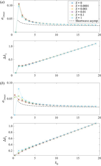
 $k_0$ up to
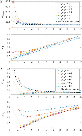
 $20$ in figure 7(a). Each cross represents a principal mode and the spectrum is discrete. The dotted line connects the principal modes with the same density ratio. Note that for different curves, the value of
 $k_0$ of the same
 $i$th principal mode will vary because the position of principal mode shifts from case to case. The first five data points of each curve correspond to the first five principal modes we showed in figure 6(c). In general, the maximum growth rate
 $\sigma _{1max}$ decreases as
 $k_0$ increases for all density ratios, and they all tend to a same value roughly
 $0.02487$ for large
 $k_0$. The increase of instability half-bandwidth is almost linear in
 $k_0$.
Maximum growth rate  $\sigma _{1max}$ and unstable half-bandwidth
 $\Delta k_1$ of principal modes
 $k_0<20$ for (a)
 $(m,m+1)=(0,1)$ and (b)
 $(m,m+1)=(5,6)$. The black dashed line is the short-wavelength asymptote (4.1) for
 $\rho _2/\rho _1=1$.

For the higher wavenumber resonance pair for  $m=5$ and
 $6$, the first five principal modes are shown in figure 6(d). The first principal mode only exists for a density ratio above
 $0.6$ because the first cograde branch of the mode for
 $m=5$ no longer crosses the first retrograde branch of the mode for
 $m=6$, as discussed earlier in § 3. We can see that the first five principal modes have maxima of the growth rate near
 $\rho _2/\rho _1=0.8\text {--}0.9$. Compared with the lower-mode resonance, that is,
 $(0,1)$, we see that the most unstable density ratio is closer to one for a higher value of
 $(m,m+1)$ pair. The maximum of the growth rate is slightly greater for large
 $m$ and the unstable half-bandwidth
 $\Delta k_1$ is much wider. We again extended the calculation for principal modes to
 $k_0 \le 20$ in figure 7(b). The result is very different compared with the
 $m=0$ case. The largest maximum growth rate and widest unstable half-bandwidth appear at
 $\rho _2/\rho _1=1$. The first principal mode with the lowest
 $k_0$ is most unstable and the growth rate decays for higher principal modes. However, for density ratios less than one, the first principal mode has the lowest maximum growth rate. The growth rate increases as
 $k_0$ increases and converges to a value of
 $0.04904$ as for the case
 $\rho _2/\rho _1=1$. The unstable half-bandwidth also converge to a value close to that of
 $\rho _2/\rho _1=1$. The short-wavelength asymptote for the growth rate for the case of
 $\rho _2/\rho _1=1$, given in (5.1) of Fukumoto & Hattori (Reference Fukumoto and Hattori2005) as
 \begin{equation} \sigma_{1max} \approx \frac{15}{64{\rm \pi}^2} +\frac{\sqrt{15}}{32k_0} \left[\frac{m}{\rm \pi}\left(\frac{21}{8}+\frac{1}{{\rm \pi}^2} \right) +\frac{1}{2}\left(-\frac{9\sqrt{15}}{64} +\frac{21}{8{\rm \pi}} +\frac{\sqrt{15}}{16{\rm \pi}^2} +\frac{1}{{\rm \pi}^3}\right) \right], \end{equation}
is plotted as a black dashed line in figures 7 and 8.
Maximum growth rate  $\sigma _{1max}$ and instability half-bandwidth
 $\Delta k_1$ for the
 $(0,1)$ resonance, (a)
 $\rho _2/\rho _1=0.2$ and (b)
 $\rho _2/\rho _1=0$. Surface tension,
 $S$, increases from
 $0$ to
 $1$. The black dashed line is the short-wavelength asymptote (4.1) for
 $\rho _2/\rho _1=1$ and
 $S=0$.

In general, the density difference affects the curvature instability of a vortex ring, but the change is only significant for the first few principal modes with smaller  $k_0$. For large
 $k_0$, the maximum growth rate and the instability half-bandwidth converge to those for
 $\rho _2/\rho _1=1$. As pointed out by Fukumoto & Hattori (Reference Fukumoto and Hattori2005), local vortex stretching in the toroidal direction (along
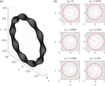
 $s$) is the mechanism for short-wavelength instability. The stretching due to the local strain field is a kinematic mechanism so that should not be affected by density. For long waves, the possible reason for increasing instability is that the fore–aft symmetry of the vortex core is broken due to the distorted boundary (p. 87 in Fukumoto & Hattori Reference Fukumoto and Hattori2005). As shown in figure 9, the sausage-like distortion and the asymmetric pressure on the vortex boundary could result in a pressure distribution in
 $s$, and this non-uniform distribution of force acts to break up the ring. In the case of a vortex core that is lighter than the outside fluid, the acceleration by the exterior pressure is amplified because the same force is acting on a smaller mass (given the same volume of the core), and the vortex becomes more unstable.
(a) The shape of disturbed boundary for the first principal mode of the  $(0,1)$ resonance at
 $(k_0,\omega _0) = (0.6647548585, 0.6183157195)$ and
 $\rho _2/\rho _1=0.4$; (b) pressure contours at different meridional cross-sections
 $k_0s$. Red curves are disturbed boundaries.

4.2. Surface tension
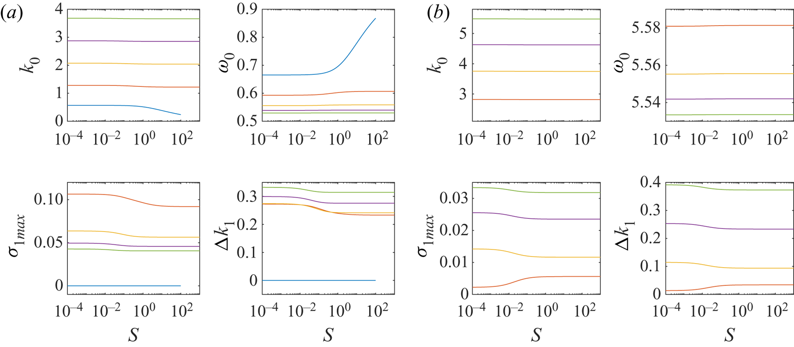
We now include surface tension  $S$ in the calculation. Adding surface tension introduces another degree of freedom into the parameter space. Calculations for the first five principal modes are shown in figure 10. In the
 $(0,1)$ case, the first principal mode (blue) is stable, while the growth rates of other four modes gradually decrease between
 $S=10^{-2}$ and
 $1$, and the second principal mode is the most unstable. The first principal mode disappears near
 $S=100$ due to the isolation of the first cograde mode from the waves for
 $m=0$ (cf. § 3). The first principal mode is absent in the
 $(5,6)$ resonance, again because of isolation. The growth rates of other four principal modes for the
 $(5,6)$ resonance vary when surface tension is less then
 $1$ but become constant when
 $S$ is greater than
 $1$. Therefore, we pick two density ratios,
 $\rho _2/\rho _1=0.2$ and
 $0$. Since (6) shows that results do not vary for
 $S>1$, we now let surface tension varies from zero to one and examine the effect of different density ratios.
First five principal modes  $(k_0,\omega _0)$ for (a)
 $(0,1)$; (b)
 $(5,6)$, the maximum growth rate
 $\sigma _{1max}$ and the instability half-bandwidth
 $\Delta k_1$ are plotted versus surface tension
 $S$.
 $\rho _2/\rho _1=0.2$. The first to fifth principal modes are blue, red, amber, purple and green curves.

The  $(0,1)$ resonant pair with no surface tension is unstable for all density ratios except for the first principal mode of
 $\rho _2/\rho _1=0.2$ (see figure 7a). Adding surface tension does not change the growth rate significantly. The growth rate of the first few principal modes decrease slightly, but for
 $k_0>6$, the growth rates are identical with different surface tension. For the density ratio
 $\rho _2/\rho _1=0$, the principal modes with higher
 $k_0$ all have the same growth rate. On the other end of the spectrum for smaller
 $k_0$, the first principal mode becomes stabilised when
 $S=1$, while the second principal mode has the largest growth rate.
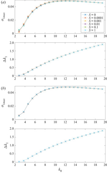
A resonant pair of higher wavenumbers  $(5,6)$ is shown in figure 11. In both figure 11(a) and 11(b), surface tension barely changes the maximum growth rate and the unstable half-bandwidth. In the short-wavelength regime, the curves for different values of surface tension collapse.
Maximum growth rate  $\sigma _{1max}$ and instability half-bandwidth
 $\Delta k_1$ for the
 $(5,6)$ resonance, (a)
 $\rho _2/\rho _1=0.2$ and (b)
 $\rho _2/\rho _1=0$. Surface tension,
 $S$, increases from
 $0$ to
 $1$.

To summarise briefly from what we have demonstrated numerically: for resonant pairs with small  $(m,m+1)$, long waves with the smallest
 $k_0$ are most unstable and the growth rate decays to a constant for large
 $k_0$. The largest growth rate occurs approximately at
 $\rho _2/\rho _1=0.2$ for the most unstable mode, and other modes have maximum growth rate between
 $\rho _2/\rho _1=0.5$ and
 $1$. Surface tension has a small influence on the instability. For a larger value of
 $(m,m+1)$ pairs, for example, the
 $(5,6)$ pair in figure 6(b), the instability is divided into two regimes around
 $\rho _2/\rho _1=0.68$: the principal mode with smallest wavenumber
 $k_0$ has the largest growth rate when the density ratio is above
 $0.68$, while it has the lowest, but non-zero, growth rate when density ratio drops below
 $0.68$. In both cases, the growth rates converge to the same value for short wavelengths, when the effect of surface tension is minimal.
4.3. Wave energy
We calculate the energy of a resonant pair of Kelvin waves using Krein's theory of parametric resonance (see Krein Reference Krein1950; MacKay Reference MacKay1986). The instability can be predicted by inspecting the energy of Kelvin waves without a calculation using the  $O(\delta \epsilon )$ dispersion relation. A formula for the wave energy is given in Cairns (Reference Cairns1979) and Fukumoto (Reference Fukumoto2003):
 \begin{equation} E^{(m)} = -\frac{\rm \pi}{2} \omega_0 \frac{\partial D}{\partial \omega_0} \left|\, f_0^{(m)} \right|^2, \end{equation}
where  $D$ is the dispersion relation obtained from (2.11) written in the form
 \begin{equation} D f_0^{(m)} \exp({\mathrm{i}(m\theta+ks-\omega t)}) =0. \end{equation}
Here
 \begin{align} D &= (\omega_0-m)^2 \left[ \frac{\rho_2}{\rho_1}\frac{(\eta_1/k_0)^2 \textrm{J}_m(\eta_1) }{m\left(1-\dfrac{2}{\omega_0-m} \right) \textrm{J}_m(\eta_1) -\eta_1 \textrm{J}_{m+1}(\eta_1)} -\frac{\textrm{K}_m}{k_0\textrm{K}_{m+1}-m\textrm{K}_m} \right] \nonumber\\ &\quad+1-\frac{\rho_2}{\rho_1} +S (m^2+k_0^2). \end{align}
This agrees with (7.6) in Fukumoto (Reference Fukumoto2003) when  $\rho _2/\rho _1=1$ and
 $S=0$. (Fukumoto (Reference Fukumoto2003) used the Bessel function of order
 $m-1$ in their formula, while we use
 $m+1$, but the two are easily verified to be equivalent.)
According to Krein's theory, the resonance between modes for  $m$ and
 $m+1$ is unstable if the cograde mode for the
 $m$ waves and the retrograde mode for
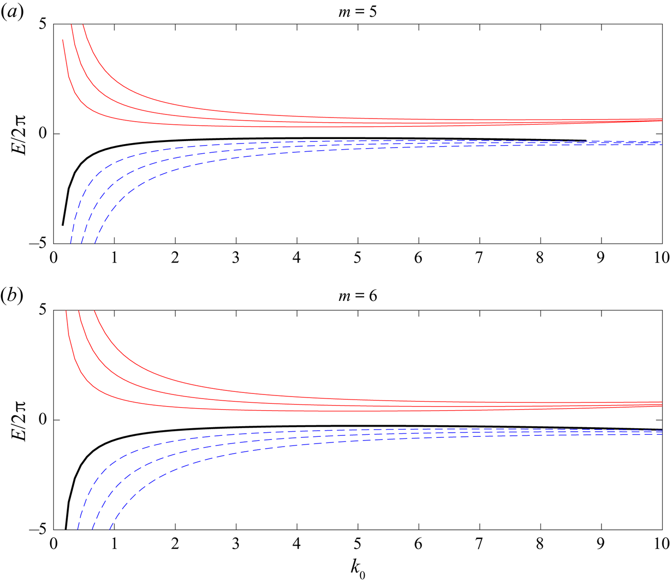
 $m+1$ waves possess energies of opposite sign, since resonance between a positive-energy and a negative-energy wave is a necessary and sufficient conditions for instability (see Fukumoto & Hattori Reference Fukumoto and Hattori2005, § 4.3). Figure 12 shows the first three cograde modes (solid red) and the first three retrograde modes (dashed blue) for
 $m=5$,
 $6$ and
 $\rho _2/\rho _1=0.1$. All the cograde modes of
 $m=5$ have positive energy while all the retrograde modes of
 $m=6$ have negative energy, therefore the first three principal modes created from their intersections are unstable.
The energy of the first three cograde modes (solid) and the first three retrograde modes (dashed) of Kelvin waves for  $m=5$,
 $6$. The solid thick line is the isolated mode. The sign of the energy of the cograde modes for
 $m=5$ and the retrograde mode for
 $m=6$ govern the stability of the
 $(5,6)$ resonance.

4.4. Non-principal modes
As discussed in § 3 and demonstrated in figure 5, changing the value of  $(\rho _2/\rho _1, S)$ from
 $(1,0)$ leads to the isolation of the first cograde branch of Kelvin wave for wavenumber
 $m$. Once it migrates out of the region of
 $\omega _0 \in (m,m+1)$, it no longer intersects the first retrograde branch of
 $m+1$. As a result the first principal mode will no longer exist, so that the sequence of principal modes now starts with the second principal mode. Our discussion and calculations so far have been limited to those principal modes.
Other than the principal modes, any intersection point of the  $i$th cograde branch for
 $m$ and the
 $j$th retrograde branch for
 $m+1$ when
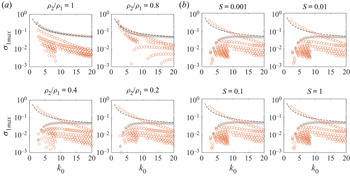
 $i\ne j$ will be called a non-principal mode. Growth rates for some non-principal modes are shown in figure 13. The nature of the instability changes with the isolation of the first cograde branch of Kelvin waves. The growth rates of principal modes are not always larger than that of non-principal modes for
 $\rho _2/\rho _1=0.8$ (figure 13a, top right) as they were in the case of
 $\rho _2/\rho _1=1$ (top left), but the first principal mode is still the most unstable. As
 $\rho _2/\rho _1$ diminishes further, the first principal mode disappears (figure 5) and the rest of the principal modes are no longer the most unstable for smaller
 $k_0$, while remaining the most unstable in
 $k_0\to 20$. The same trend can be seen in figure 13(b) for surface tension variation. The most unstable mode is the mode with the smallest value of
 $k_0$, no matter whether it belongs to the sequence of principal modes or not. This result indicates that a vortex ring is most unstable for the longest wavelength able to fit inside its circumference when subject to curvature instability given any pair of
 $(\rho _2/\rho _1, S)$.
Maximum growth rate  $\sigma _{1max}$ for the modes of the
 $(5,6)$ resonance with variations of (a)
 $\rho _2/\rho _1$ and (b)
 $S$. Principal modes are marked by blue crosses while the other modes are red circles. The black dashed line is short-wavelength asymptotic (4.1) for
 $\rho _2/\rho _1=1$ and
 $S=0$.

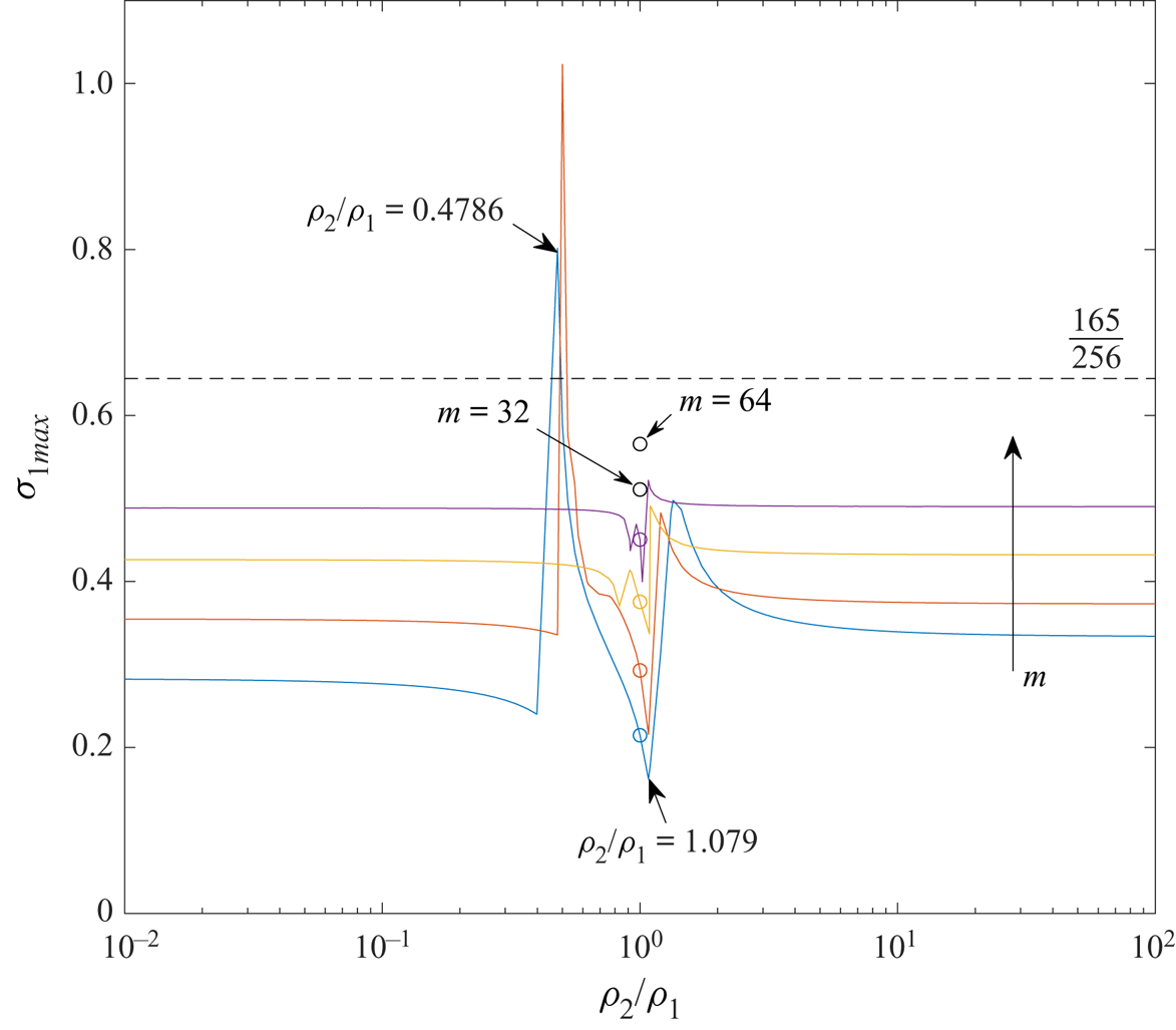
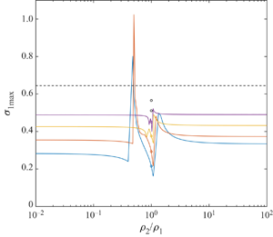
The maximum growth rate for all modes is shown in figure 14 as functions of the density ratio. The growth rate as  $m\to \infty$ for
 $\rho _2/\rho _1=1$ from Fukumoto & Hattori (Reference Fukumoto and Hattori2005) is
 $165/256= 0.64453125$ (dashed line). In our calculation for
 $\rho _2/\rho _1\ne 1$, the growth rate is not always bounded by that value. Taking
 $m=2$ for example, a cusp at
 $\rho _2/\rho _1=0.4786$ can be observed in figure 14, where
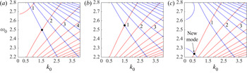
 $\sigma _{1max}=0.8013$. This can be related to the isolation of the first cograde mode from the other cograde modes for
 $m$ (see figure 15a, with the first cograde branch in the top left corner). As discussed in § 3, the isolation made the first principal mode, that is, the intersection point between the first cograde and the first retrograde modes, moves toward
 $\omega _0=m+1$. Once it has moved out of the domain
 $\omega _0\in (m,m+1)$, the first principal mode disappears and a non-principal mode has the largest growth rate. A steep drop of the curve to the left of the cusp in figure 14 correspond to this transition of the largest growth rate from a principal mode to a non-principal mode.
Maximum growth rate for modes with  $\rho _2/\rho _1 \in [0.01,100]$. Blue, red, amber and purple curves are for
 $m=2$,
 $4$,
 $8$ and
 $16$, respectively. The growth rate for
 $\rho _2/\rho _1=1$ is indicated by a circle. The dashed line is the value
 $165/256$ when
 $m\to \infty$ from Fukumoto & Hattori (Reference Fukumoto and Hattori2005).

Intersection points of pair  $(m,m+1) =(2,3)$: (a)
 $\rho _2/\rho _1=0.4083$, (b)
 $\rho _2/\rho _1=1$ and (c)
 $\rho _2/\rho _1=1.2$. Principal modes are labelled by numbers; the others are non-principal modes. The black dot is the mode that has the largest growth rate. The most unstable mode switches from point 1 to the new mode and causes the jump at
 $\rho _2/\rho _1=1.079$ in figure 14.

Another steep elevation of growth rate is observed near  $\rho _2/\rho _1=1.079$ because of a reversed version of the isolation: when
 $\rho _2/\rho _1$ increases beyond one, the isolated branch for
 $m+1$ wave migrates upward to its retrograde branches. In that case the isolated branch intersects with the cograde modes for
 $m$ wave (see figure 15c, with the isolated branch in the bottom left corner), which creates a new set of non-principal modes including one with the largest growth rate. The principal modes only possess the largest growth rate in the interval between the two ‘cliffs’ where
 $\rho _2/\rho _1 \in (0.4786,1.079)$ in figure 14, and non-principal modes have the largest growth rate in the rest of the region. The discontinuities in figure 14 may seem problematic, but they are reasonable given that the stability calculation takes a set of discrete points (the intersection points between Kelvin waves for
 $m$ and
 $m+1$) as the candidates for instability. Figure 14 shows the largest growth rate among those points, and it is not guaranteed that the largest growth rate always comes from exactly the same intersection point. The maximum growth rate will switch from mode to mode.
For other waves with wavenumber  $m>2$, the growth rate as a function of
 $\rho _2/\rho _1$ is qualitatively similar. The growth rate for
 $m=4$ has peak value
 $1.023$ at
 $\rho _2/\rho _1=0.5$ for
 $m=4$. The range of
 $\rho _2/\rho _1$ where a principal mode is most unstable becomes narrower as
 $m$ increases. In the region away from the cusp, that is,
 $\rho _2/\rho _1<0.1$,
 $\rho _2/\rho _1>10$ and
 $\rho _2/\rho _1=1$, the growth rate is independent of
 $\rho _2/\rho _1$ and gradually approaches the value of
 $165/256$ as
 $m$ increases. To the right of the plot, where
 $\rho _2/\rho _1>10$, the growth rate is higher than that to the left, where
 $\rho _2/\rho _1<0.1$, for example,
 $\sigma _{1max}=0.3341$ at
 $\rho _2/\rho _1=100$ compared with
 $0.2822$ at
 $\rho _2/\rho _1=0.01$, and they are both higher than
 $0.2146$ at
 $\rho _2/\rho _1=1$ for
 $m=2$. That indicates that a heavy core is more unstable than a light core. However, the difference shrinks as
 $m$ increases: for
 $m=8$, it is
 $\sigma _{1max}=0.4903$ to
 $0.4885$. The numerics were unable to resolve beyond wavenumber
 $m=32$ except for
 $\rho _2/\rho _1=1$.
5. Conclusion
We have carried out a linear stability analysis to investigate the density and surface tension effects on a vortex ring, which is a generalisation of the calculations of Fukumoto & Hattori (Reference Fukumoto and Hattori2005) for  $\rho _2/\rho _1=1$ and
 $S=0$. Curvature instability for the principal modes of resonances between Kelvin waves for wavenumber
 $m$ and
 $m+1$ are calculated. In the long-wavelength regime
 $k_0<10$, the instability is enhanced for the symmetric (
 $m=0$) and bending (
 $m=1$) modes when
 $\rho _2/\rho _1 \ne 1$, but is suppressed for
 $m>1$. Surface tension mitigates the instability for long waves, but the effect is minor. For the short-wavelength regime
 $k_0>10$, the effects of density and surface tension are minimal, and the principal modes are asymptotically similar to the case of
 $\rho _2/\rho _1=1$ and
 $S=0$. For all the resonances, including principal and non-principal modes, the longest wavelength is the most unstable. The principal modes are not guaranteed to be the most unstable modes for
 $(\rho _2/\rho _1, S)\ne (1,0)$.
We have presented results for a wide range of values of  $\rho _2/\rho _1$ and
 $S$. It is now of interest to consider the values of these quantities for real-world situations. These might include bubble rings in water, for which
 $\rho _2/\rho _1$ is approximately
 $0.001$. Surface tension between water and air is
 $7.2\times 10^{-3}\ \textrm {kg}\ \textrm {s}^{-2}$, and
 $S$ depends on the strength of circulation
 $\varGamma$ and the size of the ring. If we assume a thin bubble ring of diameter
 $1.5$ m and core radius 1 cm that travels roughly at
 $2\ \textrm {m}\ \textrm {s}^{-1}$,
 $S$ is of the order
 $1.8\times 10^{-4}$. Another possible example is a vortex ring made of hot air or gases, possibly formed as a thermal. The core density depends on temperature: at
 $950\,^{\circ }\textrm {C}$, the density ratio is approximately
 $0.3$. Surface tension is negligible under this circumstance. Our calculations indicate that both of these two cases are linearly unstable. The growth rate for principal modes in the former case is
 $0.09304$, a
 $70\,\%$ increase on the value
 $0.05434$ for the
 $(\rho _2/\rho _1, S)=(1,0)$ case; while the latter example has a growth rate
 $0.2807$, more than five times that of a constant-density ring.
The present work can be seen as a stepping stone to further stability analysis for a buoyant vortex ring which requires gravity in the formulation. In the present framework, we have made the ‘frozen-state’ assumption for the linear stability problem, which is justified by arguing that the Froude number is larger than the order of  $(\delta \epsilon )^{-1/2}$. It is well known that a buoyant vortex propagates in an unsteady fashion (Turner Reference Turner1957; Pedley Reference Pedley1968; Chang & Llewellyn Smith Reference Chang and Llewellyn Smith2018), so it is challenging to carry out a full analysis with gravity by the usual method of normal modes. We leave this approach to later, however, and continue with the present method to investigate density and surface tension effects on the MSTW instability in Part 2 of this work.
Acknowledgements
This work was supported by the National Science Foundation under award number CBET-1706934. C.C. thanks the Government Scholarship to Study Abroad by the Ministry of Education from Taiwan.
Declaration of interests
The authors report no conflict of interests.
Supplementary material
Supplementary materials are available at https://doi.org/10.1017/jfm.2020.845.
Appendix A. The mean flow solution
The basic solution is obtained as a perturbation series in  $\epsilon$ as shown in (2.12a–c). The leading-order solution is the Rankine vortex and the boundary is circular. Pressure is obtained from
 \begin{equation} -\frac{V_0^2}{r} = -\frac{\partial P_0}{\partial r} \end{equation}
inside and from the Bernoulli equation outside. The dynamic boundary condition for pressure on  $r=1$ gives
 \begin{equation} \frac{\rho_2}{\rho_1}P_0 +\frac{1}{2} \left(\frac{\partial \varPhi_0}{\partial \theta}\right)^2= S. \end{equation}
At  $O(\epsilon )$, the governing equations lead to
 \begin{gather} \frac{\partial U_1}{\partial \theta} -2 V_1 = -\frac{\partial P_1}{\partial r}, \end{gather}
 \begin{gather}2U_1 +\frac{\partial V_1}{\partial \theta} = -\frac{1}{r}\frac{\partial P_1}{\partial \theta}, \end{gather}
 \begin{gather}\frac{\partial U_1}{\partial r} +\frac{U_1}{r} +\frac{1}{r}\frac{\partial V_1}{\partial \theta}= -r\cos \theta \end{gather}
in the core and
 \begin{equation} \frac{\partial^2 \varPhi_1}{\partial r^2} +\frac{1}{r}\frac{\partial \varPhi_1}{\partial r} +\frac{1}{r^2}\frac{\partial^2 \varPhi_1}{\partial \theta^2} = -\frac{\cos \theta}{r} \end{equation}
outside the core. The matching conditions (2.10)–(2.11) give
 \begin{gather} U_1 = \frac{\partial F_1}{\partial \theta} = \frac{\partial \varPhi_1}{\partial r}, \end{gather}
 \begin{gather}\frac{\rho_2}{\rho_1}P_1 +\frac{\partial \varPhi_1}{\partial \theta} +F_1 \left(\frac{\rho_2}{\rho_1} -1\right) = -S \left( -\sin\theta +F_1 +\frac{\partial^2 F_1}{\partial \theta^2} \right) \end{gather}
at  $r=1$. Solving this system with the condition
 $F_1 = 0$ leads to the solution ((2.15a–c)–(2.16)).
Appendix B. The solution for Kelvin waves
Solutions to (2.23)–(2.27) with the basic state given by (2.13a,b), independent of  $s$ with wavenumber
 $m$ in
 $\theta$ and
 $k_0$ in
 $s$, are known as Kelvin waves. They take the form
 \begin{equation} \left. \begin{gathered} p_0^{(m)} = \textrm{J}_m(\eta_1r) \beta_0^{(m)}, \\ u_0^{(m)} = \frac{\mathrm{i}}{\omega_0-m+2} \left[ -\frac{m}{r}\textrm{J}_m(\eta_1r) +\frac{\omega_0-m}{\omega_0-m-2}\eta_1 \textrm{J}_{m+1}(\eta_1r) \right]\beta_0^{(m)}, \\ v_0^{(m)} = \frac{1}{\omega_0-m+2} \left[ \frac{m}{r}\textrm{J}_m(\eta_1r) +\frac{2}{\omega_0-m-2}\eta_1 \textrm{J}_{m+1}(\eta_1r) \right] \beta_0^{(m)}, \\ w_0^{(m)} = \frac{k_0}{\omega_0-m}\textrm{J}_m(\eta_1r) \beta_0^{(m)} \end{gathered} \right\} \end{equation}
for  $r<1+\tilde {f}_0$. The radial wavenumber is
 \begin{equation} \eta_1^2 = \left[\frac{4}{(\omega_0-m)^2}-1\right] k_0^2. \end{equation}
For  $r>1+\tilde {f}_0$,
 \begin{equation} \phi_0^{(m)} = \textrm{K}_m(k_0r) \alpha_0^{(m)}, \end{equation}
where  $\alpha _0$,
 $\beta _0$ are the amplitudes of Kelvin waves. The
 $(m+1)$-waves are obtained by replacing
 $m$ in the formulae by
 $m+1$. Recurrence relations are used to reduce the order of the Bessel functions.
The kinematic boundary condition (2.28) leads to
 \begin{equation} f_0^{(m)} = \frac{\mathrm{i}}{(\omega_0-m)} u_0^{(m)}. \end{equation}
The dispersion relation is obtained by enforcing the dynamic boundary condition from (3.3), which includes both surface tension and the density ratio. The resulting relation is discussed in detail in § 3.
Appendix C. Solvability conditions and dispersion relation
Substituting the  $O(\delta \epsilon )$ solutions for modes
 $m$ and
 $m+1$ into (2.36) and (2.37) gives
 \begin{equation} u_1^{(m)} = \frac{\mathrm{d} \phi_1}{\mathrm{d} r}^{(m)},\end{equation}
 \begin{align}&\frac{\rho_2}{\rho_1} p_1^{(m)} -\mathrm{i}(\omega_0-m) \phi_1^{(m)} = \mathrm{i} \omega_1\phi_0^{(m)} +\frac{m+1}{8} \left(\frac{\rho_2}{\rho_1}+4S\right)\phi_0^{(m+1)} \nonumber\\ &\quad+\left[ 1-\frac{\rho_2}{\rho_1}+S(k_0^2+m^2) \right] f_1^{(m)} +2S k_0 k_1\, f_0^{(m)} -S \left( \frac{m+1}{2}+ k_0^2 -1\right)\mathrm{i} f_0^{(m+1)} \end{align}
and
 \begin{equation} u_1^{(m+1)} = \frac{\mathrm{d} \phi_1}{\mathrm{d} r}^{(m+1)}, \end{equation}
 \begin{align}&\frac{\rho_2}{\rho_1} p_1^{(m+1)} -\mathrm{i}(\omega_0-m-1) \phi_1^{(m+1)} = \mathrm{i} \omega_1\phi_0^{(m+1)} -\frac{m}{8} \left(\frac{\rho_2}{\rho_1}+4S\right) \phi_0^{(m)} \nonumber\\ &\quad + \left[ 1-\frac{\rho_2}{\rho_1} +S(k_0^2+(m+1)^2) \right] f_1^{(m+1)} +2S k_0 k_1\, f_0^{(m+1)} -S \left( \frac{m}{2} -k_0^2 +1 \right)\mathrm{i} f_0^{(m)} \end{align}
respectively. The  $O(\delta \epsilon )$ boundary disturbance
 $f_1$ for the two modes is obtained from (2.35) as
 \begin{gather} f_1^{(m)} = \frac{1}{\mathrm{i} (\omega_0-m)} \left[ -u_1^{(m)} -\mathrm{i} \omega_1\, f_0^{(m)} -\frac{m+1}{8} f_0^{(m+1)} -\frac{5}{8}f_0^{(m+1)} \right], \end{gather}
 \begin{gather}f_1^{(m+1)} = \frac{1}{\mathrm{i} (\omega_0-m-1)} \left[ -u_1^{(m+1)} -\mathrm{i} \omega_1\, f_0^{(m+1)} +\frac{m}{8} f_0^{(m)} -\frac{5}{8}f_0^{(m)} \right]. \end{gather}
The dispersion relation relating  $k_1$ and
 $\omega _1$ for disturbances at
 $O(\delta \epsilon )$ is determined as follows. The
 $O(\delta \epsilon )$ disturbance satisfies (2.30)–(2.34) with undetermined coefficients
 $\alpha _1$,
 $\beta _1$ in the solution, which need to be determined using the boundary conditions at
 $O(\delta \epsilon )$. The boundary conditions for mode
 $m$ lead to an inhomogeneous linear system of the form
 \begin{equation} \left[ \begin{array}{cc} {\mathsf{M}}_{11} & {\mathsf{M}}_{12} \\ {\mathsf{M}}_{21} & {\mathsf{M}}_{22} \end{array} \right] \left[ \begin{array}{c} \alpha_1^{(m)} \\ \beta_1^{(m)} \end{array} \right] = \left[ \begin{array}{c} F_1 \\ F_2 \end{array} \right], \end{equation}
while the result for mode  $m+1$ becomes
 \begin{equation} \left[ \begin{array}{cc} {\mathsf{N}}_{11} & {\mathsf{N}}_{12} \\ {\mathsf{N}}_{21} & {\mathsf{N}}_{22} \end{array} \right] \left[ \begin{array}{c} \alpha_1^{(m+1)} \\ \beta_1^{(m+1)} \end{array} \right] = \left[ \begin{array}{c} G_1 \\ G_2 \end{array} \right]. \end{equation}
The vectors  $\boldsymbol {F}$ and
 $\boldsymbol {G}$ consist of the
 $O(\delta )$ solution that has undetermined coefficients
 $\alpha _0$ and
 $\beta _0$. They also depend on known quantities,
 $m$,
 $k_0$,
 $\omega _0$,
 $\rho _2/\rho _1$,
 $S$ and on the unknowns
 $k_1$ and
 $\omega _1$.
The matrices  $\boldsymbol{\mathsf{M}}$ and
 $\boldsymbol{\mathsf{N}}$ depend on
 $m$,
 $\omega _0$,
 $k_0$,
 $\rho _2/\rho _1$ and
 $S$. The two linear systems are singular, that is, their determinants are zero. The solvability condition requires that the vectors
 $\boldsymbol {F}$ and
 $\boldsymbol {G}$ lie in the image space of
 $\boldsymbol{\mathsf{M}}$ and
 $\boldsymbol{\mathsf{N}}$, that is,
 \begin{equation} \left. \begin{gathered} {\mathsf{M}}_{11} F_2 -{\mathsf{M}}_{21} F_1 = 0, \\ {\mathsf{N}}_{11} G_2 - {\mathsf{N}}_{21} G_1 = 0. \end{gathered} \right\} \end{equation}
Using the relations
 \begin{equation} \alpha_0^{(m)} = - \frac{\mathrm{i} \textrm{J}_m(\eta_1)}{(\omega_0-m)\textrm{K}_m(k_0)} \beta_0^{(m)}, \quad \alpha_0^{(m+1)} = - \frac{\mathrm{i} \textrm{J}_{m+1}(\eta_2)}{(\omega_0-m-1)\textrm{K}_{m+1}(k_0)} \beta_0^{(m+1)} \end{equation}
to replace  $\alpha _0^{(m)}$ and
 $\alpha _0^{(m+1)}$, (C 9) can be converted into a homogeneous linear system
 \begin{equation} \left[ \begin{array}{cc} {\mathsf{D}}_{11} & {\mathsf{D}}_{12} \\ {\mathsf{D}}_{21} & {\mathsf{D}}_{22} \end{array} \right] \left[ \begin{array}{l} \beta_0^{(m)} \\ \beta_0^{(m+1)} \end{array} \right] = \boldsymbol{0}. \end{equation}
For non-trivial  $\beta _0^{(m)}$ and
 $\beta _0^{(m+1)}$, the resulting determinant equation
 \begin{equation} {\mathsf{D}}_{11} {\mathsf{D}}_{22} - {\mathsf{D}}_{12} {\mathsf{D}}_{21} = 0 \end{equation}
leads to the dispersion relation for  $(k_1, \omega _1)$. This is a quadratic equation for
 $\omega _1$, where
 $\omega _1$ is obtained from
 ${\mathsf{D}}_{11}$ and
 ${\mathsf{D}}_{22}$ as
 \begin{equation} {\mathsf{D}}_{11} = \mu_1 \omega_1 +\mu_2, \quad {\mathsf{D}}_{22} = \mu_3 \omega_1 +\mu_4. \end{equation}
The dispersion relation is, hence,
 \begin{equation} \mu_1 \mu_3 \omega_1^2 +(\mu_1 \mu_4+\mu_2\mu_3) ~\omega_1+\mu_2\mu_4 - {\mathsf{D}}_{12} {\mathsf{D}}_{21} = 0. \end{equation}
Expressions for  $\mu _i$ and
 ${\mathsf{D}}_{12}$,
 ${\mathsf{D}}_{21}$ are given in the supplementary material.
These quantities are functions of  $k_1$ with
 $m$,
 $\omega _0$,
 $k_0$,
 $\rho _2/\rho _1$ and
 $S$ all given. The growth rate
 $\sigma _1 = |\mathrm {Im}{\omega _1}|$ has a maximum when
 $k_1=0$ where
 $\mu _2=\mu _4=0$, giving
 \begin{equation} \sigma_{1max} = \sqrt{-\frac{{\mathsf{D}}_{12}{\mathsf{D}}_{21}}{\mu_1 \mu_3}}. \end{equation}
One half of the unstable bandwidth  $\Delta k_1$ is calculated by finding the root
 $k_1$ of
 \begin{equation} \left(\mu_1 \mu_4+\mu_2\mu_3\right)^2 -4\mu_1 \mu_3 \left(\mu_2\mu_4 - {\mathsf{D}}_{12} {\mathsf{D}}_{21} \right)=0. \end{equation}