2.1. Governing equations

We use cylindrical coordinates $(r, \theta , z)$, with velocity $\boldsymbol {u}=(u,v,w)$. The undisturbed core boundary is taken to be $r = 1$. As the core is rotational, the governing equations for an inviscid, incompressible flow are the Euler equations inside the core,

(2.1a,b)\begin{equation} \boldsymbol{\nabla} \boldsymbol{\cdot} \boldsymbol{u} = 0, \quad \frac{\partial \boldsymbol{u}}{\partial t} +\boldsymbol{u} \boldsymbol{\cdot} \boldsymbol{\nabla} \boldsymbol{u} ={-} \boldsymbol{\nabla} p. \end{equation}

Vorticity is zero outside the core of the vortex ring, and the Laplace equation governing the velocity potential in this irrotational region is

(2.2)\begin{equation} \nabla^2 \varPhi = 0. \end{equation}

In cylindrical coordinates the Euler equations are

(2.3)\begin{gather} \frac{\partial u}{\partial t} +\boldsymbol{u} \boldsymbol{\cdot} \boldsymbol{\nabla} u-\frac{v^2}{r} ={-}\frac{\partial p}{\partial r}, \end{gather}

(2.4)\begin{gather}\frac{\partial v}{\partial t} +\boldsymbol{u} \boldsymbol{\cdot} \boldsymbol{\nabla} v+\frac{uv}{r} ={-}\frac{1}{r}\frac{\partial p}{\partial \theta}, \end{gather}

(2.5)\begin{gather}\frac{\partial w}{\partial t} +\boldsymbol{u} \boldsymbol{\cdot} \boldsymbol{\nabla} w ={-}\frac{\partial p}{\partial z}, \end{gather}

where

(2.6)\begin{equation} \boldsymbol{u} \boldsymbol{\cdot} \boldsymbol{\nabla} = u\frac{\partial}{\partial r} +\frac{v}{r}\frac{\partial}{\partial \theta}+w\frac{\partial}{\partial z}. \end{equation}

The continuity equation is

(2.7)\begin{equation} \frac{1}{r}\frac{\partial}{\partial r}(ru) +\frac{1}{r}\frac{\partial v}{\partial \theta}+\frac{\partial w}{\partial z} = 0. \end{equation}

Outside the core, Laplace's equation is

(2.8)\begin{equation} \frac{1}{r}\frac{\partial}{\partial r}\left(r\frac{\partial \varPhi}{\partial r}\right) +\frac{1}{r^2}\frac{\partial^2 \varPhi}{\partial \theta^2}+\frac{\partial^2 \varPhi}{\partial z^2} = 0. \end{equation}

The solution to (2.3) and (2.7) is called the inner solution, whereas the outer solution refers to the solution of (2.8).

2.2. Boundary conditions

The boundary of the vortex is taken to be $r=F$, where $F(\theta \; \gamma )$ will be obtained as part of the solution. The inner and outer solutions are matched on the core boundary where $r=F$. For inviscid flows, the matching is given by the kinematic and the dynamic conditions. The kinematic condition gives

(2.9)\begin{equation} \left. \frac{\textrm{D}}{\textrm{D}t}(r-F) \right |_{r=F^-} = \left. \frac{\textrm{D}}{\textrm{D}t}(r-F) \right |_{r=F^+} = 0, \end{equation}

where $\textrm {D}/\textrm {D}t=\partial /\partial t + \boldsymbol {u} \boldsymbol {\cdot } \boldsymbol {\nabla }$ is the Lagrangian time derivative.

The dynamic condition requires pressure to be continuous without surface tension or to have a jump given by surface tension. In terms of the inner pressure $p$ and outer velocity potential $\varPhi$, this becomes

(2.10)\begin{equation} \frac{\rho_2}{\rho_1} p +\frac{\partial \varPhi}{\partial t} +\frac{1}{2} |\boldsymbol{\nabla} \varPhi|^2 = S \boldsymbol{\nabla} \boldsymbol{\cdot} \boldsymbol{n}. \end{equation}

Here $S$ is dimensionless surface tension $\sigma /[\rho _1 a(\varGamma /2{\rm \pi} a)^2]$ and $\boldsymbol {n}=\boldsymbol {\nabla }(r-F)/|\boldsymbol {\nabla }(r-F)|$ is the outward normal vector on the boundary.

2.3. The mean-flow solution

The solution to (2.3)–(2.8) (written using uppercase letters) can be obtained as a perturbation series in $\gamma$:

(2.11a–c)\begin{equation} \boldsymbol{U} = \boldsymbol{U}_0 +\gamma \boldsymbol{U}_1+\cdots, \quad P = P_0 +\gamma P_1+\cdots, \quad \varPhi = \varPhi_0 +\gamma \varPhi_1+\cdots, \end{equation}

where $\gamma$ is the strength of the strain field.

The leading-order mean-flow solution is the Rankine vortex with velocity and pressure fields

(2.12a,b)\begin{equation} (U_0, V_0, W_0) = (0, r, 0), \quad P_0 = \frac{1}{2}\left(r^2-1-\frac{\rho_1}{\rho_2}\right) +\frac{\rho_1}{\rho_2}S \end{equation}

and

(2.13)\begin{equation} \varPhi_0 = \theta. \end{equation}

The strain field leads to the following $O(\gamma )$ solution of the mean flow (cf. the solution in Moore & Saffman Reference Moore and Saffman1971):

(2.14a–c)\begin{equation} U_1 ={-}r \sin{2\theta}, \quad V_1 ={-}r \cos{2\theta}, \quad P_1 = 0 \end{equation}

in the inner region, whereas the outer solution is

(2.15)\begin{equation} \varPhi_1 = \frac{1}{8}\left[ \frac{3}{r^2}-r^2 -\frac{\rho_2}{\rho_1}\left(\frac{1}{r^2}+r^2\right) +3S\left(\frac{1}{r^2}+r^2\right) \right] \sin{2\theta}. \end{equation}

The shape of the boundary to $O(\gamma )$ is

(2.16)\begin{equation} F(\theta; \gamma) = F_0 +\gamma F_1+\cdots = 1 +\gamma \frac{1}{2}\cos{2\theta} +O(\gamma^2). \end{equation}

See appendix A for the detailed calculations leading to (2.12a,b)–(2.16).

2.4. Linearised equations and boundary conditions for infinitesimal disturbances

We disturb the mean flow derived in § 2.3 as follows:

(2.17a–e)\begin{equation} U+\tilde{u}, \quad V+\tilde{v}, \quad W+\tilde{w}, \quad P+\tilde{p}, \quad \varPhi+\tilde{\phi}, \end{equation}

and the disturbed boundary is $r=F+\tilde {f}$. We use tildes over lowercase letters to represent the disturbances. Disturbances are assumed to be of $O(\delta )$ compared with the $O(1)$ basic state with $\delta \ll 1$. The usual stability analysis treats $O(\delta )$ disturbances. Here, these are neutrally stable as shown in § 3.1, and it is the $O(\delta \gamma )$ solution that is of interest for parametric instability. The disturbances are decomposed into normal modes in the axial direction $z$ and time $t$. As with the basic solution, disturbances are expanded in $\gamma$ as

(2.18)\begin{gather} \tilde{\boldsymbol{u}} = (\tilde{\boldsymbol{u}}_0 +\gamma\tilde{\boldsymbol{u}}_1 +\cdots) \exp({\mathrm{i}(kz-\omega t)}), \end{gather}

(2.19)\begin{gather}\tilde{p} = (\tilde{p}_0 +\gamma \tilde{p}_1 +\cdots) \exp({\mathrm{i}(kz-\omega t)}), \end{gather}

(2.20)\begin{gather}\tilde{\phi} = (\tilde{\phi}_0 +\gamma\tilde{\phi}_1 +\cdots) \exp({\mathrm{i}(kz-\omega t)}). \end{gather}

The axial wavenumber and the frequency are also expanded as

(2.21a,b)\begin{equation} k = k_0 +\gamma k_1 +\cdots, \quad \omega = \omega_0 +\gamma\omega_1 +\cdots. \end{equation}

The core boundary disturbance is

(2.22)\begin{equation} \tilde{f} = (\,\tilde{f}_0 +\gamma \tilde{f}_1 + \cdots) \exp({\mathrm{i}(kz-\omega t)}). \end{equation}

As the disturbances $(\tilde {\boldsymbol {u}}, \tilde {p}, \tilde {\phi })$ are small compared with the basic solution $(\boldsymbol {U}, P, \varPhi )$, (2.3)–(2.8) can investigated at $O(\delta )$ and $O(\delta \gamma )$ in what follows.

2.4.1. $O(\delta )$ linearised equations and boundary conditions

The linearised equations for disturbances at $O(\delta )$ are

(2.23)\begin{gather} {-}\mathrm{i} \omega_0 \tilde{u}_0 +\frac{V_0}{r}\frac{\partial \tilde{u}_0}{\partial \theta} -\frac{2 V_0 \tilde{v}_0}{r} ={-}\frac{\partial \tilde{p}_0}{\partial r}, \end{gather}

(2.24)\begin{gather}{-}\mathrm{i} \omega_0 \tilde{v}_0 +\tilde{u}_0\frac{\partial V_0}{\partial r} +\frac{V_0}{r}\frac{\partial \tilde{v}_0}{\partial \theta} + \frac{V_0 \tilde{u}_0}{r} ={-}\frac{1}{r}\frac{\partial \tilde{p}_0}{\partial \theta}, \end{gather}

(2.25)\begin{gather}{-}\mathrm{i} \omega_0 \tilde{w}_0 +\frac{V_0}{r}\frac{\partial \tilde{w}_0}{\partial \theta} ={-}\mathrm{i} k_0 \tilde{p}_0, \end{gather}

(2.26)\begin{gather}\frac{1}{r}\frac{\partial}{\partial r}(r \tilde{u}_0) +\frac{1}{r}\frac{\partial \tilde{v}_0}{\partial \theta}+\mathrm{i} k_0 \tilde{w}_0 =0 \end{gather}

for the inside and

(2.27)\begin{equation} \frac{1}{r}\frac{\partial}{\partial r}\left(r \frac{\partial \tilde{\phi}_0}{\partial r}\right) +\frac{1}{r^2}\frac{\partial^2 \tilde{\phi}_0}{\partial \theta^2}-k_0^2 \tilde{\phi}_0 =0 \end{equation}

for the outside. The linearised boundary conditions at $r=1$ are

(2.28)\begin{gather} {-}\mathrm{i} \omega_0\tilde{f}_0 +\frac{\partial \tilde{f}_0}{\partial \theta} = \tilde{u}_0, \end{gather}

(2.29)\begin{gather}\tilde{u}_0 = \frac{\partial \tilde{\phi}_0}{\partial r}, \end{gather}

(2.30)\begin{gather}\frac{\rho_2}{\rho_1} \tilde{p}_0 -\mathrm{i}\omega_0\tilde{\phi}_0 +\frac{\partial \tilde{\phi}_0}{\partial \theta} = \left(1-\frac{\rho_2}{\rho_1} \right) \tilde{f}_0 -S \left(\frac{\partial^2 \tilde{f}_0}{\partial \theta^2} -k_0^2\tilde{f}_0 \right). \end{gather}

The solutions are Kelvin waves given in appendix B.

2.4.2. $O(\delta \gamma )$ linearised equations and boundary conditions

We proceed to the next order in the expansion in $\gamma$. The equations for disturbances of $O(\delta \gamma )$ are also linearised. The inner solution satisfies

(2.31)\begin{align} & {-}\mathrm{i} \omega_0 \tilde{u}_1+\frac{\partial \tilde{u}_1}{\partial \theta} -2\tilde{v}_1+\frac{\partial \tilde{p}_1}{\partial r} \nonumber\\ &\quad= \left( \mathrm{i} \omega_1-\frac{\partial U_1}{\partial r}\right)\tilde{u}_0 -U_1\frac{\partial \tilde{u}_0}{\partial r}-\frac{V_1}{r}\frac{\partial \tilde{u}_0}{\partial \theta} -\left(\frac{1}{r}\frac{\partial U_1}{\partial \theta}-\frac{2V_1}{r}\right) \tilde{v}_0,\\ &{-}\mathrm{i} \omega_0 \tilde{v}_1 +2\tilde{u}_1+\frac{\partial \tilde{v}_1}{\partial \theta}+\frac{1}{r}\frac{\partial \tilde{p}_1}{\partial \theta} \nonumber\\ &\quad= \left( \mathrm{i} \omega_1-\frac{1}{r}\frac{\partial V_1}{\partial \theta}-\frac{U_1}{r}\right)\tilde{v}_0 -U_1\frac{\partial \tilde{v}_0}{\partial r}-\frac{V_1}{r}\frac{\partial \tilde{v}_0}{\partial \theta} -\left(\frac{\partial V_1}{\partial r}+\frac{V_1}{r}\right) \tilde{u}_0, \end{align}

(2.32)\begin{align} &{-}\mathrm{i} \omega_0 \tilde{w}_1+\frac{\partial \tilde{w}_1}{\partial \theta} +\mathrm{i} k_0 \tilde{p}_1 ={-}\mathrm{i} k_1 \tilde{p}_0 +\mathrm{i} \omega_1 \tilde{w}_0 -U_1\frac{\partial \tilde{w}_0}{\partial r}-\frac{V_1}{r}\frac{\partial \tilde{w}_0}{\partial \theta} \end{align}

with the continuity equation

(2.33)\begin{equation} \frac{\partial \tilde{u}_1}{\partial r} +\frac{\tilde{u}_1}{r} +\frac{1}{r}\frac{\partial \tilde{v}_1}{\partial \theta}+\mathrm{i} k_0 \tilde{w}_1 ={-}\mathrm{i} k_1 \tilde{w}_0. \end{equation}

The velocity potential outside satisfies

(2.34)\begin{equation} \frac{\partial^2 \tilde{\phi}_1}{\partial r^2}+\frac{1}{r}\frac{\partial \tilde{\phi}_1}{\partial r} +\frac{1}{r^2}\frac{\partial^2 \tilde{\phi}_1}{\partial \theta^2} -k_0^2 \tilde{\phi}_1 = 2k_0 k_1 \tilde{\phi}_0. \end{equation}

The linearised kinematic boundary conditions at $r=1$ are

(2.35)\begin{gather} {-}\mathrm{i} \omega_0\tilde{f}_1 +\frac{\partial \tilde{f}_1}{\partial \theta} -\tilde{u}_1 = \mathrm{i}\omega_1\tilde{f}_0 -V_1\frac{\partial \tilde{f}_0}{\partial \theta} -\frac{\mathrm{d} F_1}{\mathrm{d} \theta}\tilde{v}_0 +\frac{\partial U_1}{\partial r} \tilde{f}_0 +F_1 \frac{\partial \tilde{u}_0}{\partial r}, \end{gather}

(2.36)\begin{gather} \tilde{u}_1 -\frac{\partial \tilde{\phi}_1}{\partial r} = \left(-\frac{\partial \varPhi_1}{\partial \theta}+V_1 \right)\frac{\partial \tilde{f}_0}{\partial \theta} +\left( 2\frac{\mathrm{d} F_1}{\mathrm{d} \theta}+\frac{\partial^2 \varPhi_1}{\partial r^2}-\frac{\partial U_1}{\partial r} \right)\tilde{f}_0 \nonumber\\ \hspace{4.5pc} +\frac{\mathrm{d} F_1}{\mathrm{d} \theta}\left(\tilde{v}_0-\frac{\partial \tilde{\phi}_0}{\partial \theta}\right) +F_1 \left( 2\frac{\partial \tilde{f}_0}{\partial \theta}+\frac{\partial^2 \tilde{\phi}_0}{\partial r^2} -\frac{\partial \tilde{u}_0}{\partial r}\right). \end{gather}

The linearised dynamic condition at $r=1$ is

(2.37)\begin{align} & \frac{\rho_2}{\rho_1} \tilde{p}_1 -\mathrm{i}\omega_0\tilde{\phi}_1 +\frac{\partial \tilde{\phi}_1}{\partial \theta}\nonumber\\ &\quad = \mathrm{i} \omega_1\tilde{\phi}_0 -\frac{\partial \varPhi_1}{\partial r}\frac{\partial \tilde{\phi}_0}{\partial r} -\frac{\partial \varPhi_1}{\partial \theta}\frac{\partial \tilde{\phi}_0}{\partial \theta} +\left(1-\frac{\rho_2}{\rho_1} \right) \tilde{f}_1 +\left(2\frac{\partial \varPhi_1}{\partial \theta} -\frac{\partial^2 \varPhi_1}{\partial r\partial \theta}\right) \tilde{f}_0 \nonumber\\ &\qquad -F_1\left[ \frac{\rho_2}{\rho_1}\frac{\partial \tilde{p}_0}{\partial r}-\mathrm{i}\omega_0\frac{\partial \tilde{\phi}_0}{\partial r} +\frac{\partial^2 \tilde{\phi}_0}{\partial r\partial\theta} -2\frac{\partial\tilde{\phi}_0}{\partial\theta} \right] -F_1\left[\frac{\rho_2}{\rho_1} \frac{\partial^2 P_0}{\partial r^2} +3\left( \frac{\partial \varPhi_0}{\partial\theta}\right)^2 \right] \tilde{f}_0 \nonumber\\ &\qquad -S \left(\frac{\partial^2 \tilde{f}_1}{\partial \theta^2}-k_0^2\,\, \tilde{f}_1 -2k_0 k_1 \tilde{f}_0 -2 F_1\frac{\partial^2 \tilde{f}_0}{\partial \theta^2} \right). \end{align}

Solutions for the disturbance waves at $O(\delta )$ and $O(\delta \gamma )$ are given in the next section. The dispersion relation is obtained by matching the boundary conditions.

3.1. Kelvin waves at $O(\delta )$

The solution at $O(\delta )$ is a Kelvin wave, which is described in appendix B. The Kelvin waves are coupled with the quadrupole field (2.14a–c) through the right-hand sides of (2.31)–(2.33). When two Kelvin waves with azimuthal wavenumber $m$ and $m+2$ appear in the forcing terms on the right-hand side of (2.31)–(2.33), the solution at the $O(\delta \gamma )$ will possess modes for $m-2$, $m$, $m+2$ and $m+4$. The resonances are between pairs of two adjacent modes separated by two. We focus on the resonance between a pair of Kelvin waves $(m,m+2)$ in this paper, because the cases for $(m-2,m)$, $(m+2,m+4)$ can be obtained by using different value of $m$.

The solution (B1) and (B4) contains coefficients (Kelvin wave amplitudes) $\alpha _0$ and $\beta _0$ that are determined using the boundary conditions. The boundary conditions for wavenumber $m$ become

(3.2)\begin{gather} {-}\mathrm{i}(\omega_0-m) f_0^{(m)} = u_0^{(m)} = \frac{\mathrm{d} \phi_0}{\mathrm{d} r}^{(m)}, \end{gather}

(3.3)\begin{gather}\frac{\rho_2}{\rho_1} p_0^{(m)} -\mathrm{i} (\omega_0 -m) \phi_0^{(m)} = \left(1-\frac{\rho_2}{\rho_1} \right) f_0^{(m)} +S (m^2+k_0^2) f_0^{(m)}. \end{gather}

Substituting $p_0^{(m)}$, $u_0^{(m)}$, $\phi _0^{(m)}$ and $f_0^{(m)}$ (see appendix B) into the equations above, we obtain a set of homogeneous linear equations for $\alpha _0^{(m)}$ and $\beta _0^{(m)}$. For non-trivial $\alpha _0^{(m)}$ and $\beta _0^{(m)}$, the determinant must be zero, which gives the dispersion relation for mode $m$ (see Part 1):

(3.4)\begin{align} & \left[ 1 +\frac{E_1}{(\omega_0-m)^2} \left(m -k_0 \frac{\textrm{K}_{m+1}(k_0)}{\textrm{K}_{m}(k_0)}\right) \right] \textrm{J}_{m+1}(\eta_1) \nonumber\\ &\quad = \left\{{-}m\frac{\omega_0-m}{\omega_0-m+2} +\left[\frac{\rho_2}{\rho_1}-E_1 \frac{m}{(\omega_0-m)(\omega_0-m+2)}\right] \left(m -k_0 \frac{\textrm{K}_{m+1}(k_0)}{\textrm{K}_{m}(k_0)}\right) \right\}\nonumber\\ &\qquad \times \frac{\eta_1}{k_0^2}\textrm{J}_{m}(\eta_1), \end{align}

where $E_1 = 1-\rho _2/\rho _1 +S(k_0^2+m^2)$. Here $\textrm {J}_m$ is the Bessel function of the first kind and $\textrm {K}_m$ is the modified Bessel function of the second kind; $\eta _1$ is the radial wavenumber defined in (B2). For the second set of Kelvin waves, the azimuthal wavenumber is $m+2$ in the MSTW instability instead of $m+1$ in the curvature calculation. The boundary conditions are the same formulae as in (3.3) except that $m$ is replaced by $m+2$, and similarly for the solution in appendix B. Using the boundary conditions and the solution for the $m+2$-mode, we obtain the dispersion relation

(3.5)\begin{align} & \left[ 1 - \frac{E_2}{(\omega_0-m-2)^2} \left(m+2 +k_0 \frac{\textrm{K}_{m+1}(k_0)}{\textrm{K}_{m+2}(k_0)}\right) \right] \textrm{J}_{m+1}(\eta_2) \nonumber\\ &\quad = \left\{-(m+2)\frac{\omega_0-m-2}{\omega_0-m-4} +\left[\frac{\rho_2}{\rho_1}+E_2 \frac{m+2}{(\omega_0-m-2)(\omega_0-m-4)}\right]\right.\nonumber\\ &\qquad \times \left.\left(m+2 +k_0 \frac{\textrm{K}_{m+1}(k_0)}{\textrm{K}_{m+2}(k_0)}\right) \right\} \frac{\eta_2}{k_0^2}\textrm{J}_{m+2}(\eta_2), \end{align}

where $E_2 = 1-\rho _2/\rho _1 +S[k_0^2+(m+2)^2]$ and $\eta _2$ is the radial wavenumber for $m+2$.

The intersection points between the two sets of Kelvin waves give possible candidates for parametric instability. The actual modes can be found by finding the roots for (3.4) and (3.5) with $\omega _0 \in [m,m+2]$. For Kelvin waves with azimuthal wavenumber $m$, there are cograde branches going upward where $\omega _0>m$ and retrograde branches going downward where $\omega _0 < m$ (see figure 2 for $m=2$). The cograde branches are labelled from the top as the first, second, $\ldots$ cograde modes, whereas the retrograde branches are labelled from the bottom. The cograde branches of the $m$ waves and the retrograde branches of the $m+2$ waves cross in $\omega _0 \in [m,m+2]$ setting up possible modes for resonance. We follow the definition used by Fukumoto (Reference Fukumoto2003) for the case $(\rho _2/\rho _1,S)=(1,0)$. The principal modes are the intersection point of the first cograde branch for $m$ and the isolated branch for $m+2$, and also the intersection points of the $i+1$th cograde branches for $m$ and the $i$th retrograde branches for $m+2$. This definition is slightly different from that in § 3 of Part 1 for the curvature instability, where the cograde branches for $m$ never cross the isolated branch for $m+1$ when $(\rho _2/\rho _1,S)=(1,0)$.

Figure 2.

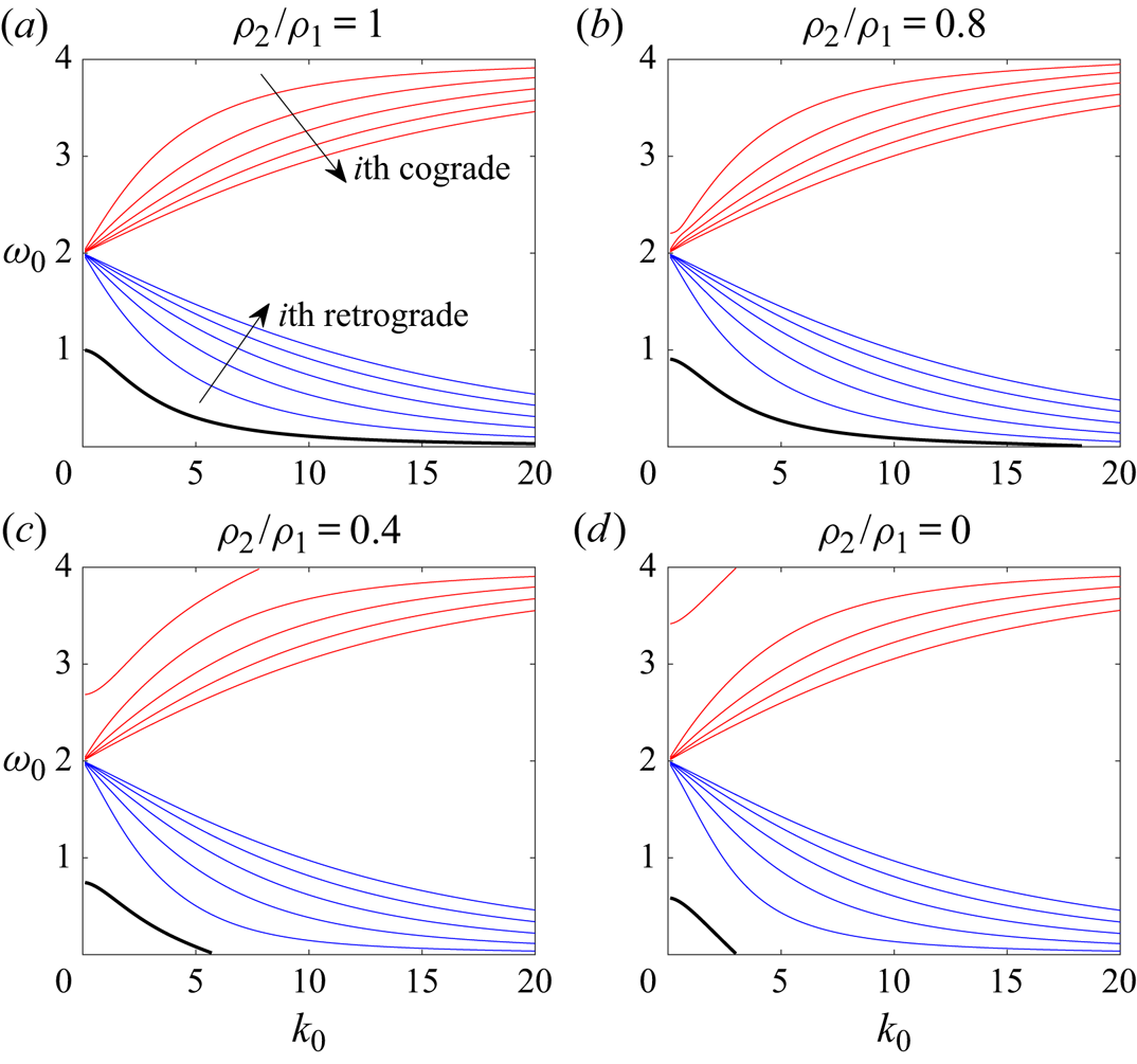
Dispersion curves for the Kelvin wave with $m=2$ for density ratios from one to zero. Red curves are cograde branches and blue curves are retrograde branches. Only the first five branches of each are plotted. An isolated branch (thick black curve) can be seen below the retrograde branches. Surface tension is zero for all plots.

As discussed in Part 1, density and surface tension act to ‘isolate’ the first cograde mode when $(\rho _2/\rho _1,S)\ne (1,0)$. In figure 2, the first cograde mode (the uppermost red curve with the largest value of $|\omega _0-2|$) departs from the other cograde modes and shifts upward as the density ratio decreases. The isolated branch (thick black line) also shifts downward from its initial position when $\rho _2/\rho _1=1$, and the short-wavelength part (large $k_0$) of the isolated branch drops below $\omega _0=m-2$. On the other hand, when the density ratio increases above one, the situation reverses: the first cograde mode and the isolated mode move closer toward other cograde and retrograde modes. In all cases, Kelvin waves stay neutrally stable. 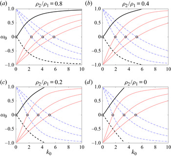The branch that extends beyond $\omega _0 \in [m-2,m+2]$ still has purely real $\omega _0$. A special scenario is two counter-winding helical waves with azimuthal wavenumber $m=-1$ and $1$ whose dispersion curves are symmetric about the $k_0$-axis (figure 3). In this case, the principal modes are always on the $k_0$-axis, and $\omega _0=0$.

Figure 3.

The first three cograde modes of the Kelvin wave for $m=-1$ (red) and the first three retrograde modes of the Kelvin wave for $m=1$ (blue dashed); their isolated branches (thick solid and dashed) can be seen emanating from $(k_0,\omega _0)=(0,0)$. Circles are the first four principal modes with $\omega _0=0$. Here $S=0$ for all cases.

3.2. Resonance at $O(\delta \gamma )$

The solution of the $O(\delta \gamma )$ disturbances governed by (2.31)–(2.34) is given in appendix A of Fukumoto (Reference Fukumoto2003). We do not reproduce it here, given its complexity. The solution contains undetermined coefficients $\alpha _1$, $\beta _1$ (appearing in the linear systems in (C7) and (C8)) which must be non-zero. The boundary conditions in (2.37) and (2.38) are used to obtain the dispersion relation. Note that in order to include surface tension, we need to compute $\tilde {f}_1$ from (2.36) before using the dynamic condition for the dispersion relation. In Moore & Saffman (Reference Moore and Saffman1975), Tsai & Widnall (Reference Tsai and Widnall1976) and Fukumoto (Reference Fukumoto2003), computing $\tilde {f}_1$ is not necessary because $\rho _2/\rho _1=1$ and surface tension is omitted.

Substituting the basic solution (2.14a–c)–(2.16) into the boundary conditions (2.37) and (2.38) gives

(3.6)\begin{align} \tilde{u}_1 -\frac{\partial \tilde{\phi}_1}{\partial r} &= \sin2\theta \left[ \frac{\partial \tilde{\phi}_0}{\partial \theta}-\tilde{v}_0+\left(1-\frac{\rho_2}{\rho_1}+3S\right)\tilde{f}_0 \right] \nonumber\\ &\quad +\frac{1}{2}\cos 2\theta \left[-\left(1-\frac{\rho_2}{\rho_1}+3S\right) \frac{\partial \tilde{f}_0}{\partial \theta}+\frac{\partial^2 \tilde{\phi}_0}{\partial r^2} -\frac{\partial \tilde{u}_0}{\partial r}\right]; \end{align}

(3.7)\begin{align} &\frac{\rho_2}{\rho_1} \tilde{p}_1 -\mathrm{i}\omega_0\tilde{\phi}_1 +\frac{\partial \tilde{\phi}_1}{\partial \theta} \nonumber\\ &\quad = \mathrm{i} \omega_1\tilde{\phi}_0 +\sin2\theta \frac{\partial \tilde{\phi}_0}{\partial r} +\left(1-\frac{\rho_2}{\rho_1} \right) \tilde{f}_1 -\frac{1}{2}\left({-}1-\frac{\rho_2}{\rho_1}+3S\right)\cos2\theta \frac{\partial \tilde{\phi}_0}{\partial \theta} \nonumber\\ &\qquad +\frac{3}{2}\left( 1-\frac{\rho_2}{\rho_1}+2S \right)\cos2\theta \tilde{f}_0 -\frac{1}{2} \cos2\theta \left[ \frac{\rho_2}{\rho_1}\frac{\partial \tilde{p}_0}{\partial r}-\mathrm{i}\omega_0\frac{\partial \tilde{\phi}_0}{\partial r} +\frac{\partial^2 \tilde{\phi}_0}{\partial r\partial\theta} \right] \nonumber\\ &\qquad -S \left(\frac{\partial^2 \tilde{f}_1}{\partial \theta^2}-k_0^2 \tilde{f}_1 -2k_0 k_1 \tilde{f}_0 -\cos2\theta ~\frac{\partial^2 \tilde{f}_0}{\partial \theta^2}\right). \end{align}

Using the above equations, we obtain two sets of equations for $m$ and $m+2$ in (C1)–(C4). They can be written as two inhomogeneous linear systems (C7) and (C8) for $\alpha _1$ and $\beta _1$. The dispersion relation (C14) is given by requiring that $\alpha _1$ and $\beta _1$ do not vanish (see the details in appendix C). A dispersion relation for $(k_1,\omega _1)$ determines the stability, and the flow is unstable for $\mathrm {Im}\{\omega _1\}>0$. The maximum growth rate $\sigma _{1max}$ is given by the maximum imaginary part of $\omega _1$ at $k_1=0$; and the half-bandwidth of instability, $\Delta k_1$, by the range over which the imaginary part of $\omega _1$ does not vanish. The expressions for all formulae are too cumbersome to handle manually, and so computer symbolic algebra is utilised to obtain the dispersion relation (C14) and $\omega _1$ and $\Delta k_1$. A description of procedure is given in detailed in appendix C, and the symbolic algebra files are provided in the supplementary material available at https://doi.org/10.1017/jfm.2020.1157 (as Matlab scripts). We show numerical results for $m=-1$ and $1$ in the next section, followed by the case for $m\geqslant 0$ in § 5.

4.1. Principal modes ($\omega _0=0$)

We substitute $m=-1$ and $\omega _0=0$ for the principal modes of stationary waves (circles in figure 3). The maximum growth rate $\sigma _{1max}$ and half the instability bandwidth $\Delta k_1$ are then calculated using computer symbolic algebra. To verify the result of the symbolic calculation, results for $(\rho _2/\rho _1,S)=(1,0)$ are compared with those in Fukumoto (Reference Fukumoto2003) in table 1. The present study has $\sigma _{1max}$ accurate to 10 significant figures and $\Delta k_1$ up to five significant figures. As seen in figure 3, the first principal mode at $(k_0,\omega _0)=(0,0)$ is independent of $\rho _2/\rho _1$ and $S$, so we do not include it in the comparison here.

Table 1.

For the $m=-1$ and $1$ resonances, present results for $\rho _2/\rho _1=1$ compared with table 1 of Fukumoto (Reference Fukumoto2003). Each row represents a principal mode with $k_0=0$.

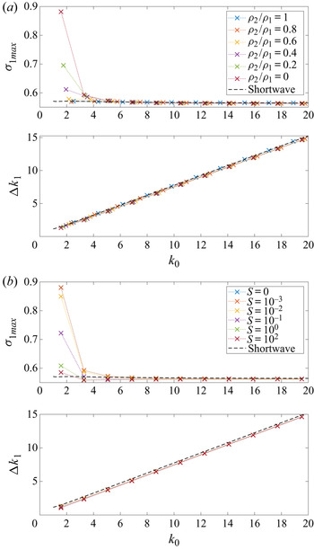
The principal modes’ maximum growth rates and instability half-bandwidths are plotted as functions of $\rho _2/\rho _1$ in figure 4(a) for $S=0$. The second principal mode (blue curve) is the most unstable mode. The largest growth rate is at $\rho _2/\rho _1=0$ with a value of $\sigma _{1max}= 0.882$. The least unstable density ratio is $0.915$, where the second and third principal modes have a growth rate of $0.5696$. The instability half-bandwidth, $\Delta k_1$, is strongly correlated with the axial wavenumber $k_0$, and the principal mode with higher $k_0$ has wider instability bandwidth. Figure 4(b) shows the effect of surface tension when $\rho _2/\rho _1=0.001$. The density ratio $0.001$ is picked because it is close to the typical ratio between air and water. Surface tension merely changes the locations of principal modes. The second principal mode dominates the instability. The growth rate is $0.8803$ at $S=10^{-4}$ and drops to $0.585$ when $S=500$.

Figure 4.

Principal modes $(k_0, 0)$ for $(m,m+2) = (-1,1)$, the maximum growth rate $\sigma _{1max}$ and the instability half-bandwidth $\Delta k_1$ plotted versus: (a) density ratio $\rho _2/\rho _1 \in [0.005,100]$ for $S=0$; (b) surface tension $S \in [0,500]$ with $\rho _2/\rho _1=0.001$. The second to sixth principal modes are the blue, red, amber, purple and green curves.

The growth rate and the instability half-bandwidth are calculated for large $k_0$ in figure 5 with different values of $\rho _2/\rho _1\in [0,1]$ and $S\in [0,100]$. Density only has an effect on the growth rate $\sigma _{1max}$ for principal modes with $k_0<10$. The growth rates for different values of $\rho _2/\rho _1$ and $S$ all converge to a fixed value $0.5625$ as $k_0\to \infty$. The short-wavelength limit given in (5.13), (5.14) of Fukumoto (Reference Fukumoto2003) for $(\rho _2/\rho _1,S)=(1,0)$ as

(4.1a)\begin{gather} \sigma_{1max} \approx \frac{9}{16} \left( 1+\frac{1}{12k_0}-\frac{7}{48k_0^2}+\frac{5}{64k_0^3} \right), \end{gather}

(4.1b)\begin{gather}\Delta k_1 \approx \frac{3 k_0}{4} \left( 1+\frac{1}{3k_0}+\frac{5}{24k_0^3} \right), \end{gather}

is plotted as dashed lines in figure 5.

Figure 5.

Maximum growth rate $\sigma _{1max}$ and unstable half-bandwidth $\Delta k_1$ of principal modes with axial wavenumber $k_0<20$ for helical waves $(m,m+2)=(-1,1)$: (a) different $\rho _2/\rho _1$ with $S=0$; (b) different $S$ with $\rho _2/\rho _1=0.001$. The dashed line is the short-wavelength asymptotic result (4.1) for $\rho _2/\rho _1=1$ and $S=0$.

4.2. Non-principal modes

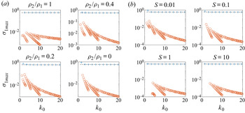
For stationary waves $m=\pm 1$, non-principal modes are intersection points where $\omega _0\ne 0$. Theoretically, an infinite number of non-principal modes exist because the two Kelvin waves have an infinite number of intersection points. Here we show only those non-principal modes for $k_0\in [0,20]$ and $\omega _0 \in (0,0.5]$ in figure 6. In the case $\rho _2/\rho _1=1$ and $S=0$, the growth rates of non-principal modes are at least two orders of magnitude smaller than that of the principal modes (see figure 6a). As the density ratio decreases to zero, the maximum growth rates of non-principal modes grow and become one order of magnitude smaller than those of the principal modes. The trend reverses for increasing surface tension. The maximum growth rate of non-principal modes is one order of magnitude less than that of the principal modes and that difference widens to more than two orders of magnitude for $S=10$ in figure 6(b). With variations in either density or surface tension, the instability of the principal modes always dominates over non-principal modes.

Figure 6.

Maximum growth rate $\sigma _{1max}$ for the modes of the $(-1,1)$ resonance with variations of (a) $\rho _2/\rho _1$ for $S=0$ and (b) $S$ for $\rho _2/\rho _1=0.001$. Principal modes (with $k_0\leqslant 20$) are marked by blue crosses whereas other modes are red circles. The black dashed line is the short-wavelength asymptotic result (4.1) for $\rho _2/\rho _1=1$ and $S=0$.

5.1. The case $m=0$

We calculate the growth rate $\sigma _{1max}$ and half the unstable bandwidth $\Delta k_1$ for the first five principal modes. The definition of principal modes is the same as in Éloy & Le Dizès (Reference Éloy and Le Dizès2001) and Fukumoto (Reference Fukumoto2003): the first principal mode is the intersection between the first cograde mode for $m=0$ and the isolated mode for $m=2$, the second principal mode is the second cograde mode for $m=0$ intersected by the first retrograde mode for $m=2$, and so on. The location $(k_0,\omega _0)$ of the principal modes in figure 7(a) shows that $k_0$ shifts to lower wavelengths as the density ratio $\rho _2/\rho _1$ drops below one. The growth rate of the first principal mode has a cusp at $\rho _2/\rho _1 = 0.215$ with $\sigma _{1max} \approx 4.32$. The mode is then stable below $\rho _2/\rho _1 < 0.215$, and this mode does not exist for $\rho _2/\rho _1 \lesssim 0.09$ because the two branches on which the first principal mode is located do not cross each other when the density ratio drops below $0.09$ (as explained in § 3.1). The third principal mode is the most unstable with $\sigma _{1max}=0.5668647793$ for $\rho _2/\rho _1 =1$ in the calculation of Fukumoto (Reference Fukumoto2003). In our calculation with density variations, the second principal mode is the most unstable mode as $\rho _2/\rho _1 \to 0$ with $\sigma _{1max} = 0.6028$, whereas the first principal mode is the most unstable for $\rho _2/\rho _1 \to 100$ with $\sigma _{1max}=0.6167$. The trend in $\Delta k_1$ is very similar to that in $k_0$: as the density ratio decreases the unstable bandwidth decreases. We also extend our calculation to other principal modes with higher axial wavenumber $k_0$ in figure 9. The growth rate is asymptotically close to that of (4.1) in the short-wavelength regime for $\rho _2/\rho _1 =1$. For large $k_0$, $\Delta k_1$ increases linearly with $k_0$ and the slopes are identical except for $k_0<4$.

Figure 7.

Principal modes for $(m,m+2) = (0,2)$, maximum growth rate $\sigma _{1max}$ and the instability half-bandwidth $\Delta k_1$ plotted versus: (a) density ratio $\rho _2/\rho _1 \in [0.005,100]$ for $S=0$; (b) surface tension $S \in [0,500]$ at $\rho _2/\rho _1=0.2$. The first to fifth principal modes are the blue, red, amber, purple and green curves.

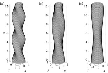
The disturbed boundary of the first principal mode in the $(0,2)$ resonance is shown in figure 8. The shape of the resonant disturbance transitions from helical waves to bulging waves as density ratio decreases. The axial wavelength of the disturbance increases ($k_0$ decreases) as the density ratio decreases. This is due to the effect of density on the Kelvin wave dispersion relation. Consequently the location of the intersection point changes. Given that the strain field is applied uniformly along the $z$-direction, bulging modes (figure 8c) are more susceptible to the strain field. Because a bulging mode is axisymmetric with respect to the $z$-axis, it has no preferred direction and can deform more easily. For helical modes, the twist makes the core structure vary constantly per unit length in $z$, so that the core is more resistant to a strain of uniform direction.

Figure 8.

Disturbed boundary for the first principal mode of the $(0,2)$ resonance with different density ratio: (a) $\rho _2/\rho _1=1$, $(k_0,\omega _0)=(1.242233570,0.8326707800)$; (b) $\rho _2/\rho _1=0.4$, $(k_0,\omega _0)=(0.7529505549,0.6784320753)$; (c) $\rho _2/\rho _1=0.22$, $(k_0,\omega _0)=(0.5503572727,0.6335367950)$. The disturbance transitions from helical mode into bulging mode as $\rho _2/\rho _1$ decreases.

Figure 9.

Maximum growth rate $\sigma _{1max}$ and unstable half-bandwidth $\Delta k_1$ of principal modes with axial wavenumber $k_0<20$ for $(m,m+2)=(0,2)$ with different $\rho _2/\rho _1$ with $S=0$. The dashed line is the short-wavelength asymptotic result (4.1) for $\rho _2/\rho _1=1$.

The dependence on surface tension $S$ is shown in figure 7(b) for $\rho _2/\rho _1=0.2$. The first principal mode does not exist as surface tension increases to a value above $S \approx 0.14$ and is always unstable below that threshold. The effect on the other four principal modes is not significant. The second principal mode (red curve) has the biggest drop in $\sigma _{1max}$ from a value of $0.6049$ to $0.5482$ at $S=100$. The mitigation of the instability by surface tension is as expected, since surface tension makes the interface more resistant to deformation when subjected to a strain.

5.2. Other pairs $(m,m+2)$

Moving on to higher resonance pairs, e.g. $(m,m+2)=(4,6)$, we found the change in the positions $(k_0,\omega _0)$ of principal modes (see figure 10a) to be qualitatively similar to that for the $(0,2)$ pair. The first principal mode (in blue in figure 10) disappears near a larger density ratio at the value of $\rho _2/\rho _1=0.72$. The most significant difference is how the growth rate behaves before the first principal mode disappears. For $(m,m+2)=(0,2)$, the growth rate of the first principal mode increases drastically and then drops to zero before the first principal mode vanishes (figure 7a), whereas for $(m,m+2)=(4,6)$, $\sigma _{1max}$ plunges to zero in figure 10(a) and never exceeds $0.6$. The dependence on surface tension $S$ is shown in figure 10(b). The growth rate $\sigma _{1max}$ decreases only slightly, and is almost independent of surface tension for $S \gtrsim 1$.

Figure 10.

Principal modes for $(m,m+2) = (4,6)$, the maximum growth rate $\sigma _{1max}$ and the instability half-bandwidth $\Delta k_1$ are plotted versus: (a) density ratio $\rho _2/\rho _1 \in [0.01,100]$ for $S=0$; (b) surface tension $S \in [0,100]$ at $\rho _2/\rho _1=0.2$. The first to fifth principal modes are the blue, red, amber, purple and green curves.

Resonance pairs with higher azimuthal wavenumber $m$ have smaller growth rate $\sigma _{1max}$ for the MSTW instability, whereas the curvature instability is more unstable for larger $m$ (see Chang & Llewellyn Smith Reference Chang and Llewellyn Smith2021). In figure 11 we plot the maximum growth rate among intersection points (resonant modes) that include the principal modes and a few non-principal modes for axial wavenumber $k_0 \leqslant 20$, as a function of density ratio $\rho _2/\rho _1$. The maximum growth rate decreases as $m$ increases. This is due to the strain field, which kills the small-scale disturbances on the boundary. 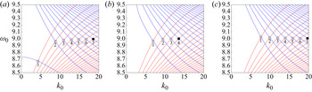For a fixed value of $m$, the growth rate is constant for very large and small $\rho _2/\rho _1$, and the curve has a dip in the middle at $\rho _2/\rho _1=0.925$. That is where the most unstable mode (that with the largest growth rate) jumps from one intersection point of Kelvin waves to another. As shown in figure 12, the most unstable mode, represented by a black dot, switches from the seventh principal mode to the fourth principal mode as the density ratio increases from $0.925$ to $1.069$.

Figure 11.

Maximum growth rate for modes with $\rho _2/\rho _1 \in [0.01,100]$ and $S=0$. Blue, red, amber and purple curves are for resonance pairs $(m,m+2)$, $m=2$, $4$, $8$ and $16$, respectively. The vertical dashed line is the value $\rho _2/\rho _1=0.925$ where the growth rate has a dip.

Figure 12.

Intersection points of the pair $(m,m+2) =(8,10)$: (a) $\rho _2/\rho _1=0.925$; (b) $\rho _2/\rho _1=1.069$; and (c) $\rho _2/\rho _1=10$. Surface tension is zero. Principal modes are labelled by numbered circles; the black dot is the mode with largest growth rate. The most unstable mode switches from the seventh principal mode to the fourth principal mode, then back to the seventh, causing the discontinuity in $\sigma _{1max}$.

Given that the whole calculation is based on discrete intersection points of Kelvin waves, the largest growth rate among all modes can have a discontinuity while it switches from one intersection point to another. That happens when the previous most unstable mode had decayed or disappeared, and another mode takes over. The instability of a resonant mode is a function of its location $(k_0,\omega _0)$ and the location is a function of density ratio and surface tension. The migrations of the first cograde mode and the isolated mode discussed in § 3 also have a huge influence on the location of intersection points.