A. Costly Labor Adjustment

One implication of Diamond (Reference Diamond1982) is that firms in environments with greater matching efficiency grow faster, as they face lower adjustment costs and fewer informational frictions in aligning workers with jobs. These frictions matter because labor turnover is costly: whenever a firm adjusts its workforce, it incurs expenses from firing, search, selection, hiring, and training (e.g., Oi (Reference Oi1962), Shapiro (Reference Shapiro1986)). Faced with such costs, a firm may rationally retain an unproductive worker whose wage exceeds their output or forego hiring a worker whose short-term productivity exceeds their wage (Blanchard and Portugal (Reference Blanchard and Portugal2001)).

In addition to the direct turnover costs, empirical evidence suggests that firms also incur significant indirect costs of labor adjustment, such as reduced productivity (Autor, Kerr, and Kugler (Reference Autor, Kerr and Kugler2007)), costs of financial distress (Agrawal and Matsa (Reference Agrawal and Matsa2013)), accumulation of precautionary cash (Ghaly et al. (Reference Ghaly, Anh Dang and Stathopoulos2017)), and a high degree of operating leverage (Klasa et al. (Reference Klasa, Ortiz-Molina, Serfling and Srinivasan2018)). Greater matching efficiency lowers the costs of labor adjustment. A competitive employer can fill vacancies quickly, reducing search and hiring expenses while minimizing production and financial losses. By easing these frictions, efficient matching directly supports faster firm growth.

B. Ex Ante Investment Hold Up

Information friction inevitably exists in a labor market because workers and firms lack complete information about each other to predict the probability of a successful job-worker match. This information friction creates a hold-up problem when irreversible capital investments must be made before hiring: workers are unwilling to invest in new skills when the wage premium depends on finding a firm with new technology, and firms are unwilling to invest in technology when the profitability depends on finding skilled labor to operate (Acemoglu (Reference Acemoglu1997)). As a result, job vacancy risk can reduce the optimal investment return (Acemoglu (Reference Acemoglu1998), Acemoglu and Shimer (Reference Acemoglu and Shimer1999)).

Higher matching efficiency also alleviates hold-up problems by improving information for both workers and firms about the likelihood of a successful match. In Acemoglu’s (Reference Acemoglu1997) model, which assumes no technological externalities nor aggregate demand spillovers, firms are more likely to invest in technology where more workers are looking for a job, and workers are more likely to train for new skills where more employers are hiring (Rotemberg and Saloner (Reference Rotemberg and Saloner2000), Lazear (Reference Lazear2009), and Moretti (Reference Moretti2010)). Thus, matching efficiency fosters growth not only by lowering adjustment costs but also by encouraging greater investment. Taken together, these mechanisms predict that a firm’s labor-matching efficiency in its local market has a positive effect on growth.

A. Establishment Data: NETS

Our primary source for establishment-level data is the National Establishment Time-Series (NETS) database, maintained by Dun & Bradstreet. This comprehensive data set provides detailed information, including addresses, for every U.S. establishment owned by public and private entities over the period of 1990–2020. More importantly, the dataset is free from survivorship bias and has a strong correlation with the U.S. Census data. We construct plant-level sales and employment from this data set. We are also able to identify an extensive margin of corporate restructuring activities, such as plant closure and divestiture statuses. NETS includes unique parent- and establishment-level identifiers, allowing researchers to trace ownership information of establishments. It is important to mention a caveat that comes with the application of the NETS data. Crane and Decker (Reference Crane and Decker2020) find that, despite the strong correlation with the Current Employment Statistics (CES) and Quarterly Census of Employment and Wages (QCEW), NETS tends to oversample establishments with fewer than 10 employees. Therefore, we exclude these small establishments to mitigate the bias.

B. Measurement of Labor Matching Efficiency (LME)

We aim to construct an empirical proxy for the likelihood that an establishment can recruit qualified workers from the local labor market. Intuitively, the relevant measure is likely to depend not only on the size of a metropolitan area but also on the skill set required for the production function of the establishment. For instance, a software company may be more likely to find desired software engineers in the San Jose-Sunnyvale-Santa Clara MSA than in the Houston-The Woodlands-Sugar Land MSA, even though the latter is roughly 3.5 times larger in terms of the labor market size based on the 2020 census. We incorporate these considerations in our construction of the measure.

Our data source for labor matching efficiency is the Occupational Employment and Wage Statistics (OEWS) from the U.S. Bureau of Labor Statistics (BLS) for the period of 1999–2020. OEWS uses a standard occupational classification (SOC) system that includes 822 detailed occupational categories, covering near-universal job categories in the public, private, and military sectors. These data are released at various levels (e.g., national, state, industry, and MSA), and we use the revised categories whenever BLS makes those available. We began our sample in 1999, when the OEWS program started providing the most granular occupation definitions.Footnote ⁵

We construct this measure in four steps: first, we use occupational data at industry level from the OEWS to construct an industry-level employee composition vector, $ {V}_{i,t} $ , for industry i in year t, where an element of $ {V}_{i,t} $ is the proportion of labor in industry i assigned to occupation k. Footnote ⁶ We use 6-digit SIC codes up to 2001 and 6-digit NAICS codes from 2002 for industry classification. Because our unit of analysis is the establishment, we infer establishment-level occupational composition using NAICS industry-level data as the fine-grained industry classification mitigates concerns regarding the accuracy of labor matching inference.

Second, we use the occupational data at the MSA level from the OEWS to construct a MSA-level employee composition vector, $ {V}_{m,t} $ for the MSA m in year t, where an element of $ {V}_{m,t} $ is the proportion of labor in the MSA m assigned to the occupation k. Third, we use the angular separation of the two vectors, $ {V}_{i,t} $ and $ {V}_{m,t} $ , to calculate a cosine similarity between the labor-skill compositions of an industry and those of an MSA. Specifically, the cosine similarity is the scalar product of the two vectors divided by the product of their lengths:

(1) $$ Cosine\hskip0.22em {Similarity}_{i,m,t}=\frac{V_{i,t}{V}_{m,t}^{\prime }}{\sqrt{V_{i,t}{V}_{i,t}^{\prime }}\sqrt{V_{m,t}{V}_{m,t}^{\prime }}}. $$

Cosine Similarity in equation (1) is bounded between 0 and 1, where 0 (1) means that the industry and MSA-level employee compositions have no (perfect) similarities. In our final step, we create the labor matching efficiency (LME) variable by standardizing the cosine similarity in equation (1) to simplify interpretation of the results.Footnote ⁷ We explain the construction of the Cosine Similarity in Section B of the Supplementary Material.

We assign the LME to each establishment based on its industry–MSA–year combination. Specifically, we map establishments’ ZIP codes from the NETS to MSAs from the OEWS using the ZIP code–MSA crosswalk provided by the Office of Workers’ Compensation Programs (OWCP) of the U.S. Department of Labor.Footnote ⁸

C. Summary Statistics

Table 1 reports summary statistics. The sample in Panel A comprises 398,196 plant-year observations from 33,517 establishments and 21,268 parent corporations over the 1999–2020 period. On average, each parent firm operates 1.81 subsidiary establishments. The Cosine Similarity averages 0.26 (bounded between 0.10 and 0.55), implying that most establishments face partial but not perfect alignment with their local skill pool—exactly what one would expect in a frictional labor market. Establishments in higher-similarity terciles exhibit systematically larger employment and sales, higher Paydex scores, and lower bankruptcy incidence as shown in Panel D. For example, bankruptcy probability falls from 1.3% in the lowest tercile to 0.2% in the highest, while sales and employment rise monotonically.

TABLE 1Summary Statistics

TABLE 1 Long description

Panel A. Establishment-Level Sample (398,196 observations for most variables):

* Cosine Similarity: Mean 0.262, Median 0.244, Std. Dev. 0.097, Min. 0.096, Max. 0.553.

* L M E: Mean 0, Median -0.187, Std. Dev. 1, Min. -1.717, Max. 3.010.

* Employment: Mean 187.792, Median 80, Std. Dev. 434.541, Min. 10, Max. 19,000.

* Log(Emp): Mean 4.443, Median 4.394, Std. Dev. 1.158, Min. 2.303, Max. 7.433.

* Sales ($ millions): Mean 42.630, Median 14.026, Std. Dev. 155.980, Min. 0.865, Max. 6,845.119.

* Log(Sales): Mean 16.500, Median 16.456, Std. Dev. 1.395, Min. 11.800, Max. 20.047.

* Paydex (360,431 obs): Mean 67.346, Median 69, Std. Dev. 10.322, Min. 0, Max. 99.

* Bankruptcy: Mean 0.006, Median 0, Std. Dev. 0.077, Min. 0, Max. 1.

* Closure: Mean 0.043, Median 0, Std. Dev. 0.204, Min. 0, Max. 1.

* Divestiture: Mean 0.056, Median 0, Std. Dev. 0.229, Min. 0, Max. 1.

Panel B. N B E R - C E S Manufacture Sample (378 observations):

* C A P E X / C S: Mean 0.067, Median 0.066, Std. Dev. 0.022, Min. 0.022, Max. 0.128.

* T F P: Mean -0.0004, Median 0.003, Std. Dev. 0.037, Min. -0.115, Max. 0.104.

Panel C. COMPUSTAT Sample (33,459 observations):

* C A P E X / T A: Mean 0.054, Median 0.043, Std. Dev. 0.046, Min. 0.004, Max. 0.284.

* C A P E X / P P E: Mean 0.179, Median 0.081, Std. Dev. 0.275, Min. 0.004, Max. 1.688.

Panel D. Univariate Distribution of Key Variables Sorted by L M E Terciles (T1 low, T2, T3 high):

* Log(Emp): T1 4.403, T2 4.432, T3 4.495.

* Log(Sales): T1 16.423, T2 16.522, T3 16.555.

* Paydex: T1 66.920, T2 67.339, T3 67.781.

* Bankruptcy: T1 0.013, T2 0.003, T3 0.002.

Graph A of Figure 1 shows that manufacturing establishments account for the bulk of observations, a setting where workforce alignment is especially salient for studying how local labor markets shape firm outcomes. Graph B highlights that our proposed employee–firm match index exhibits meaningful time-series variation rather than being a sticky, slow-moving construct. This property is central to our identification strategy: if cosine similarity were largely fixed within industry–MSA pairs, any correlation with growth could be dismissed as reflecting permanent advantages or static firm sorting across locations. Instead, the observed evolution of Cosine Similarity over 1999–2020 indicates that local labor–firm fit responds systematically to shifts in occupational demand and supply.

FIGURE 1Establishment-Level Sector Shares and Time-Series Variation in Cosine Similarity, 1999–2020

Figure 1 displays sectoral composition and time-series patterns of the NETS sample. Graph A reports establishment-level sector shares, while Graph B plots the time-series variation in Cosine Similarity. Both private and public establishments are included. The sample covers 1999–2020, with sectors defined by 2-digit NAICS industry classifications.

FIGURE 1 Long description

Graph A. Sector Distribution is a pie chart showing five categories. Manufacturing is the dominant sector at 85.24 percent. Moving clockwise, the remaining sectors are Trade at 8.04 percent, Services at 3.15 percent, Transportation at 2.15 percent, and Other at 1.43 percent.

Graph B. Time-Series Variation of Cosine Similarity is a line graph with the X-axis labeled Year from 1999 to 2020 and the Y-axis labeled Cosine Similarity ranging from 0.22 to 0.3. The data begins in 1999 at approximately 0.276, drops to 0.26 in 2000, and peaks near 0.295 in 2001. From 2001 to 2004, the value remains high between 0.29 and 0.295. A steady decline begins in 2005, reaching a local low of approximately 0.246 in 2010. The value stabilizes around 0.25 until 2015, then drops sharply to its lowest point of approximately 0.232 in 2017. The graph concludes with a slight recovery, ending at approximately 0.247 in 2020.

A. Validating the LME

We begin our analysis by investigating the relationship between our labor matching efficiency proxy and local business activity. Labor market theories posit that in regions with thick labor markets, firms experience faster growth and higher wages due to reduced labor adjustment costs, which are redistributed as higher wages to retain employees (Oi (Reference Oi1962)). If our measure effectively captures the alignment between establishment labor demand and local labor supply, we expect a positive association between labor matching efficiency and these outcomes.

We rely on County Business Patterns (CBP), an annual series that provides local economic data by industry of the establishment. The CBP is constructed primarily from administrative records of the Internal Revenue Service (IRS) and the Social Security Administration (SSA), supplemented by Census Bureau surveys to ensure accuracy in establishment counts, employment, and payroll. The data are systematically validated and aggregated across multiple statistical units. A key advantage for our setting is that the CBP reports consistently at the industry–MSA level, which mitigates concerns that inference is confounded by establishment-specific heterogeneity and instead allows us to capture variation at the relevant local industry margin.

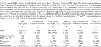
Table 2 presents the results. We use total employment and number of establishments as proxies for local business activities. Columns 1 and 2 indicate that LME is positively and significantly related to business growth at the industry–MSA level. The inclusion of MSA-by-year and industry-by-year fixed effects alleviate concerns that time-varying shocks at either the location or industry drive the estimates. Columns 4 and 5 show that these relations remain economically meaningful when outcomes are expressed in logarithms. A one-standard-deviation increase in LME is associated with a 29.1% increase in total employment and a 17.3% increase in the number of establishments.Footnote ⁹

TABLE 2Validation Using County Business Patterns Sample

TABLE 2 Long description

The table consists of 6 numbered columns and 6 primary data rows.

Column Headers:

1. Total Employees

2. Total Number of Establishments

3. Total Annual Payroll in 1,000 dollars

4. Log Total Employees

5. Log Total Number of Establishments

6. Log Total Annual Payroll

Data Rows:

- L M E: Coefficients for models 1 through 6 are 5,036.815 (standard error 1,364.16), 172.823 (standard error 75.69), 481,805.8 (standard error 11,503.8), 0.291 (standard error 0.026), 0.173 (standard error 0.016), and 0.331 (standard error 0.030). Statistical significance is indicated by asterisks.

- Industry-year F E: Yes for all columns.

- M S A-year F E: Yes for all columns.

- Number of observations: 24,834 for all columns.

- Adjusted R-squared: Values are 0.472, 0.433, 0.339, 0.818, 0.942, and 0.788 respectively.

- Mean of Dependent Variable: Values are 24,600.82, 1,586.28, 1,297,069, 8.82, 5.67, and 12.65 respectively.

An alternative interpretation to the above results is that our results may reflect the influence of dominant employers or industry clusters, rather than labor matching effect. In such cases, large firms or clusters could simultaneously drive both measured LME and local growth. To assess this possibility, columns 3 and 6 incorporate payroll-based outcomes. We find that LME is positively associated with average industry wages within an MSA. This pattern is inconsistent with the monopsony hypothesis, under which a dominant employer or concentrated set of firms would suppress wages below competitive levels due to limited worker outside options (Bhaskar, Manning, and To (Reference Bhaskar, Manning and To2002), Berger, Herkenhoff, and Mongey (Reference Berger, Herkenhoff and Mongey2022)).

Taken together, the evidence indicates that the positive relation between LME and local establishment growth is not an artifact of employer dominance or clustering. Rather, the results support the interpretation that LME captures genuine improvements in labor market efficiency, with economically meaningful implications for local growth.

B. OLS Results – Establishment Level

Next, we turn to our main analysis and use establishment-year panel data. Specifically, we estimate the following empirical equation using OLS regression:

(2) $$ {Growth}_{i,t+1}={\beta}_0+{\beta}_1\times {LME}_{i,t}+{\unicode{x025B}}_{i,t+1}, $$

where Growth is proxied by one of the following two variables: natural logarithm of employment, log(emp), and natural logarithm of sales, log(sales). The variable of interest, LME, is the standardized cosine similarity between establishments’ operating industry and MSA.

Table 3 presents the regression results of equation (2). Columns 1–3 present the results with log(emp) and columns 4–6 present the results with log(sales) as the dependent variables. The coefficients across all columns are statistically significant and economically meaningful. For example, a one-standard-deviation increase in LME is associated with a 2.0% increase in the employment and a 1.9% increase in total revenues.

TABLE 3OLS Panel Regression

TABLE 3 Long description

A regression table with six columns numbered 1 through 6. Columns 1 to 3 use Log Emp as the dependent variable, and columns 4 to 6 use Log Sales.

* Row 1: L M E coefficients. Model 1 is 0.019 with three asterisks. Model 2 is 0.019 with three asterisks. Model 3 is 0.020 with two asterisks. Model 4 is 0.021 with three asterisks. Model 5 is 0.019 with three asterisks. Model 6 is 0.019 with one asterisk.

* Row 2: Standard errors for L M E. Model 1 is 0.004. Model 2 is 0.005. Model 3 is 0.010. Model 4 is 0.004. Model 5 is 0.006. Model 6 is 0.010.

* Fixed Effects: Plant F E and Industry-year F E are Yes for all models. M S A-year is No for models 1 and 4, and Yes for models 2, 3, 5, and 6. Parent-year is No for models 1, 2, 4, and 5, and Yes for models 3 and 6.

* Summary Statistics: Number of observations is 398,196 for all models. Adjusted R-squared values range from 0.924 in Model 1 to 0.943 in Model 6.

Our baseline results control for establishment fixed effects. Hence, any cross-sectional differences that are time invariant are not driving the results. We also account for local shocks, such as those caused by directed policy interference or economic fluctuations, by including a vector of MSA-by-year fixed effects in columns 2 and 5 of Table 3 in addition to plant and industry-by-year fixed effects. We, therefore, estimate the effect of labor matching efficiency on establishment-level growth, conditional on the average effect of local shocks. Finally, we control for parent firm-level shocks. For example, two establishments owned by the same parent firm may be subject to similar production functions, financial constraints, and business decisions at the parent level. We take advantage of this setting by interacting with a full set of parent-by-year fixed effects in columns 3 and 6 in addition to plant, industry-by-year, and MSA-by-year fixed effects, so that the effect on establishment growth is relative to other establishments with the same parent.Footnote ¹⁰

Overall, the findings reinforce the idea that access to quality employees is helpful for firm growth, particularly for businesses that depend significantly on labor in their production function.

C. Alternative Empirical Specifications

In this section, we substantiate the validity of our findings through a series of robustness tests. We also address potential omitted variable bias at the establishment level, which could confound the interpretation of LME as a driver of firm growth.

1. Does Initial Economic Condition Explain the Results?

Prior studies suggest that initial economic conditions signal firm quality and predict future performance (Guzman and Stern (Reference Guzman and Stern2020), Maksimovic, Phillips and Yang (Reference Maksimovic, Phillips and Yang2023)). Here, we would like to understand whether our baseline results stem from heterogeneous economic conditions across establishments within the same $ MSA\times industry $ cells, which will be the level at which our LME measure varies.

We include the initial size-MSA-year fixed effects in addition to establishment fixed effects, industry-by-year fixed effects, and parent-by-year fixed effects. The added fixed effects ensure that our analyses compare the effect of LME on establishment growth between establishments located in the same MSA that experience similar initial economic influence at the start of our sample but with different exposure to labor market pool. We measure initial establishment economic condition using total employment at the sample’s inception.Footnote ¹¹ The establishments are grouped into quintiles based on total employment.

Columns 1 and 2 of Table 4 report the results for log(emp) and log(sales), respectively. The point estimates increase by approximately 30% (= 0.026/0.02 −1) relative to the baseline results. This pattern suggests that baseline estimates are attenuated by systematic differences in growth trajectories across establishment economic condition categories within local labor markets. Large and small establishments in the same MSA–year can face very different scaling constraints, such that larger establishments expand more slowly because they are closer to capacity, while smaller plants often grow more rapidly in the same booming local markets.

TABLE 4OLS – Alternative Specification

TABLE 4 Long description

The table consists of 10 columns divided into five pairs representing different specifications.

1. Initial Size-M S A-Year F E (Columns 1 and 2): L M E coefficients are 0.026 and 0.025 respectively.

2. Excluding Largest 20% Plants (Columns 3 and 4): L M E coefficients are 0.022 and 0.027.

3. Excluding Industry Cluster (Columns 5 and 6): L M E coefficients are 0.017 and 0.019.

4. Rank Based on 10 Deciles (Columns 7 and 8): L M E coefficients are 0.017 and 0.015.

5. Randomly Assigned L M E (Columns 9 and 10): L M E coefficients are -0.007 and -0.007.

Dependent variables alternate between Log of Emp and Log of Sales for most groups, except for the Rank group which uses Rank of Emp and Rank of Sales.

Fixed Effects (F E) included across almost all models: Plant F E, Industry-year F E, and Parent-year F E. M S A-year F E is included in columns 3 through 10. Initial size-M S A-Year F E is only included in columns 1 and 2.

Observation counts range from 318,594 to 398,196. Adjusted R-squared values are high, ranging from 0.931 to 0.956.

A. The Instrumental Variable Approach

To address these residual concerns, we rely on a strict leave-one-out (LOO) instrumental variable (IV) approach. This IV reconstructs the national occupational profile by excluding the focal MSA and then measures its alignment with other MSAs. By design, it removes the mechanical feedback between an establishment’s own labor decisions and the LME, ensuring that local shocks do not enter the instrument. The identifying variation arises only from how the national skill-demand vector tilts when the focal unit is omitted, which is orthogonal to local industry–MSA–year shocks. Intuitively, when other MSAs’ labor profiles shift in a way that moves the purged national vector closer to a focal MSA, cosine similarity rises—but this shift is driven entirely by conditions outside the focal market. The IV therefore addresses the simultaneity that neither fixed effects nor robustness checks can remove, delivering plausibly exogenous variation in national skill alignment. Our LOO is constructed in the following way:

(3) $$ {Z}_{i,m,t}^{\mathrm{LOO}}=\frac{1}{M-1}\sum \limits_{m^{\prime}\ne m}\cos \left({V}_{i,t}^{-m},{V}_{m^{\prime },t}\right). $$

To satisfy the exclusion restriction, the industrial composition of MSAs must not disproportionately influence the purged national vector. This condition in turn will be true as long as sector is not concentrated in a particular MSA, a condition we verify at the 2-digit NAICS level (Blanchard and Katz (Reference Blanchard and Katz1992)).Footnote ¹⁴ We assess sector concentration using the Herfindahl–Hirschman Index (HHI), computed across MSAs based on three proxies: total establishments, employment, and revenue. As reported in Panel A of Table 5, the mean HHI ranges from 0.031 to 0.050, indicating that, on average, sector concentration is low (below 5%). This provides strong evidence that no single industry overwhelmingly drives labor demand within MSAs. Additionally, the median HHI ranges between 7 and 8 basis points, reinforcing the finding of limited concentration. While the 95th percentile of the distribution reveals some MSAs with higher concentration, these outliers are further excluded in our specifications.

TABLE 5Instrumental Variable Estimation

TABLE 5 Long description

Panel A, Sector Concentration in M S As (2-digit S I C), lists three variables: Sector H H I (establishments), Sector H H I (E M P), and Sector H H I (S A L E S). For each, it provides Mean, 5th, 25th, 50th, 75th, and 95th Percentiles. Mean values range from 0.031 to 0.050, with the 95th percentile showing the highest concentration at 0.231 for Sales.

Panel B, First and Second Stage I V Estimates, contains 10 columns. Columns 1 and 2 use the Full Sample, while columns 3 through 10 exclude the top 5 percent concentration. The dependent variables are Log(Emp) and Log(Sales).

In the 2 S L S Estimates with Fixed Effects section:

* Instrumented L M E coefficients are positive and significant across all columns, ranging from 0.033 to 0.044.

* Bartik I V controls for technology adoption, input-output connection, and labor mobility are included in specific columns (5-10) but are generally not statistically significant.

In the First-Stage Estimates section:

* L O O L M E shows a consistent coefficient of 0.254 to 0.257, all significant at the 1 percent level.

* Kleibergen-Paap F-statistic ranges from 151.35 to 162.88.

* All models include Plant F E, Industry-year F E, M S A-year F E, and Parent-year F E.

* Number of observations is 398,196 for the full sample and 378,286 for the restricted sample.

Panel B of Table 5 reports the results of the IV estimation. The first-stage relationships are statistically strong across all specifications, with large F-statistics confirming instrument relevance for LME. The 2SLS estimates are both economically and statistically significant. In columns 1 and 2, using the full sample, a one-standard-deviation increase in instrumented LME raises employment by 3.6% and revenues by 3.3%. To address potential concentration bias, we exclude the top 5th percentile of concentrated observations in columns 3 and 4. The results remain robust, with coefficients increasing by 19% and 9%, respectively, relative to the full-sample estimates. These larger effects mirror the OLS estimates from specifications that exclude the largest establishments, consistent with attenuation rather than identification hinging on a few dominant markets.

To test robustness to potential violations of the exclusion restriction, we add time-varying covariates that could confound the identifying variation. First, we construct a Bartik-style instrument, Bartik IV Technology Adoption using detailed capital input data from BEA/BLS integrated industry production accounts. This instrument interacts industry-level technological capital expenditure contributions to output growth with initial industry labor shares in each MSA, capturing heterogeneous exposure to technology diffusion. Similarly, we build Bartik IV Input–Output Connection (Menzly and Ozbas (Reference Menzly and Ozbas2010)) and Bartik IV Labor Mobility (Donangelo (Reference Donangelo2014)) by interacting initial industry labor shares with supplier–customer linkages from BEA Benchmark I/O tables and industry-level labor mobility measures, respectively. These proxies account for potential confounding from production-network spillovers and cross-MSA labor flows. As reported in columns 5–10 of Panel B of Table 5, the 2SLS coefficients remain highly significant at the 5% level and are virtually unchanged across specifications, confirming that our results are robust to these alternative sources of variation and supporting the validity of the exclusion restriction.

In summary, our identification exploits plausibly exogenous variation in LME generated by national shifts in industry–occupation profiles driven by other MSAs. Using this source of variation, we find positive and significant effects of LME on growth. Reassuringly, the 2SLS estimates align with the OLS results, particularly regarding the heterogeneous effects of establishment size on growth.

B. A Natural Experiment – Hurricane Katrina

Our second identification strategy exploits the exogenous labor supply shock to Houston following Hurricane Katrina. The evacuation increased the population of the Houston MSA by roughly 3.1%, with most evacuees leaving the city within 2 years (McIntosh (Reference McIntosh2008), De Silva, McComb, Moh, Schiller, and Vargas (Reference De Silva, McComb, Moh, Schiller and Vargas2010)). This sudden and unanticipated influx thickened Houston’s labor market by expanding the pool of effective workers.

Following the methodology in McIntosh (Reference McIntosh2008) and Ghaly et al. (Reference Ghaly, Anh Dang and Stathopoulos2017), we construct a treatment group of establishments located in the Houston MSA and a control group of propensity-score-matched establishments in nearby MSAs that were unaffected by Katrina. The treatment group consists of establishments located in the Houston metropolitan area (Houston–The Woodlands–Sugar Land, TX). The control group comprises propensity-score-matched establishments located in other metropolitan areas of Texas and neighboring states (Arkansas, New Mexico, and Oklahoma), excluding Louisiana. We drop MSAs directly struck by the storm as well as indirectly affected areas that experienced more than a 1% population increase due to evacuee migration. We match establishments by their 6-digit NAICS code. We define post as an indicator equal to 1 for the year following Hurricane Katrina and 0 for the preceding year, as earlier evidence suggests that most evacuees returned within 2 years.

Columns 1 and 4 of Table 6 provide strong evidence that establishments in the Houston MSA experienced sizable increases in both employment and revenues following Hurricane Katrina. Using a short event window and the fixed effects effectively raises the bar for alternative explanations. Any alternative explanations must account for the observed growth in establishments located in the Houston MSAs relative to other geographically unaffected establishments, through channels that are not associated with the labor migration events.

TABLE 6Hurricane Katrina Shock

TABLE 6 Long description

The table presents regression results for two dependent variables: Log of Emp (columns 1 to 3) and Log of Sales (columns 4 to 6).

For each dependent variable, results are split into three samples: Full Sample, Manufacturing Only, and Others.

Key Data Points:

* Treat times Post: For Log of Emp, coefficients are 0.044 (Full), 0.050 (Manufacturing), and 0.023 (Others). For Log of Sales, coefficients are 0.046 (Full), 0.059 (Manufacturing), and 0.003 (Others). Standard errors are provided in parentheses below each coefficient.

* Fixed Effects: All models include Plant F E and Industry-year F E.

* Number of observations: 4,447 for Full Sample, 3,529 for Manufacturing Only, and 918 for Others.

* Adjusted R super 2: Values range from 0.969 to 0.983 across all columns.

Statistical significance is indicated by asterisks, with three asterisks denoting the highest level of significance.

One potential concern is that Hurricane Katrina did not directly shift our LME measure, but rather altered the composition of the local labor pool, implying heterogeneous shocks across industries depending on their occupational mix. In particular, low-skill, labor-intensive manufacturing sectors are more likely to have benefited from the influx, whereas high-skill industries may have experienced little improvement or even weaker matching (De Silva et al. (Reference De Silva, McComb, Moh, Schiller and Vargas2010)).

To address this concern, we first validate our identification strategy by employing a first-stage difference-in-differences test to confirm that Hurricane Katrina measurably impacted the LME variable. As shown in Table C2 in the Supplementary Material, we find that the hurricane-induced labor influx led to a significant increase in LME for Houston establishments.

While this concern is partially mitigated by the fact that manufacturing accounts for roughly 85% of our observations, we explicitly test for heterogeneity by reporting results separately for manufacturing and nonmanufacturing establishments in columns 2–3 and 5–6 of Table 6, respectively. Consistent with the labor matching mechanism, the estimated effects are concentrated among manufacturing establishments, where occupational structures are more closely aligned with evacuee inflows. In contrast, the effects are essentially absent in the nonmanufacturing subsample. Importantly, the “first-stage” effect is also concentrated within the manufacturing sector (column 2 of Table C2 in the Supplementary Material), consistent with the sector-specific nature of the labor shock.

A. Labor Adjustment Costs

1. Financial Distress Costs

We examine credit risk and restructuring events as key indicators of financial distress. To measure credit risk, we use the Paydex score from NETS, which ranges from 0 to 100 and reflects a firm’s trade credit performance. Prior research shows that the Paydex score is a strong predictor of business failure. Following Dun & Bradstreet guidelines, we also construct an indicator variable, $ {I}_{\mathrm{Paydex}\ge 80} $ , which equals 1 if a plant’s Paydex score is at least 80 and identifies low-risk establishments. Finally, we use the NETS bankruptcy flag, $ {I}_{\mathrm{Bankruptcy}} $ , as a direct measure of financial distress.

To capture restructuring costs, we focus on plant closures and divestitures, which represent extensive-margin adjustments and constitute some of the most radical responses to adverse labor market conditions. Specifically, we classify an establishment as divested if it is sold to another firm in year t and as closed if year t is its final year of existence in NETS.

Table 7 presents the results. Overall, we find that higher LME is associated with lower credit risk. In column 1, which includes plant and industry-by-year fixed effects, the LME coefficient is 0.329 and statistically significant at the 1% level. The coefficient remains statistically significant at the 5% level after MSA-by-year fixed effect is added. Columns 3 and 4 suggest that higher LME is associated with the likelihood of having a Paydex score of 80 or higher. In column 3, with establishment and industry-by-year fixed effects, the coefficient on LME is 0.011. Importantly, this estimate is virtually unchanged when MSA-by-year fixed effects are included in column 4. The economic magnitudes of the effect are nontrivial. A one-standard-deviation increase in LME corresponds to a 24% (=0.011/0.0457) reduction in financial risk, that is, a higher likelihood of being classified as low risk relative to the mean.

TABLE 7Financial Distress Costs

TABLE 7 Long description

The table is divided into two main sections: Credit Risk (Models 1 through 4) and Corporate Restructuring (Models 5 through 8).

* Column Headers:

- Models 1 and 2: Paydex Score.

- Models 3 and 4: Indicator for Paydex score greater than or equal to 80.

- Models 5 and 6: Bankruptcy.

- Model 7: Plant Closure.

- Model 8: Plant Divestiture.

* Row Data for L M E (Standard errors in brackets):

- Model 1: 0.329 (0.067)

- Model 2: 0.187 (0.083)

- Model 3: 0.011 (0.001)

- Model 4: 0.011 (0.002)

- Model 5: minus 0.003 (0.0004)

- Model 6: minus 0.002 (0.0005)

- Model 7: minus 0.004 (0.001)

- Model 8: minus 0.002 (0.001)

* Fixed Effects (F E):

- Plant F E: Yes for Models 1 through 6; No for Models 7 and 8.

- Industry-year F E: Yes for all models.

- M S A-year F E: No for Models 1, 3, and 5; Yes for Models 2, 4, 6, 7, and 8.

* Summary Statistics:

- Number of observations: 360,431 for Models 1 through 4; 398,196 for Models 5 through 8.

- Adjusted R-squared: Ranges from 0.022 (Model 8) to 0.422 (Model 2).

Next, we examine the effect of labor matching efficiency on the likelihood that an establishment goes out of business. Column 5 of Table 7 includes plant and industry-by-year fixed effects, while column 6 further adds MSA-by-year fixed effects. In both specifications, the coefficients on LME are negative and statistically significant at the 1% level, indicating that higher labor matching efficiency reduces the probability of bankruptcy. Because bankruptcy events are rare in our sample (0.6% of plant-year observations), we interpret the economic magnitudes with caution. For example, in column 6, the coefficient of −0.002 implies that a one-standard-deviation increase in LME is associated with a 33% (= −0.002/0.006) reduction in the likelihood of plant bankruptcy relative to the mean, consistent with the economic magnitudes documented in Akey and Appel (Reference Akey and Appel2021).

Finally, columns 7 and 8 of Table 7 examine plant closure and divestiture. In column 7, the coefficient on LME is −0.004 and significant at the 1% level, implying that a one-standard-deviation increase in LME lowers the likelihood of plant closure by 9% (= −0.004/0.043) relative to the mean. Column 8 shows a similar effect for plant divestiture: the coefficient on LME is −0.002, indicating a 3.5% (= −0.002/0.056) decline in the likelihood of divestiture. These results reinforce the prediction that stronger labor matching reduces the probability of both closures and divestitures. Taken together, the evidence in Table 7 corroborates the theoretical prediction that enhanced employee–firm matching alleviates financial distress, thereby fostering greater stability in employment and revenue growth.

2. Hiring Frictions

We next examine the heterogeneous effects of local labor market exposures on growth conditional on labor adjustment costs. Our hypothesis is that the mitigating role of LME becomes more pronounced when hiring frictions are elevated. To test this prediction, first we exploit exogenous variation in hiring frictions arising from the staggered adoption (or rejection) of the Inevitable Disclosure Doctrine (IDD) by state courts. The IDD allows courts to restrict employee mobility when a new role is likely to lead to the disclosure of a former employer’s trade secrets (Klasa et al. (Reference Klasa, Ortiz-Molina, Serfling and Srinivasan2018)). If LME reduces labor adjustment costs by improving employee–firm matching, then its effect on establishment growth should be amplified in states and periods subject to IDD.

We extend our baseline specification by interacting LME with an IDD indicator in a difference-in-differences framework. In addition to plant and industry-by-year fixed effects, we estimate a specification with state-by-year fixed effects to absorb unobserved state-level shocks that may coincide with changes in courts’ IDD positions and establishment growth. We incorporate parent-by-year fixed effects to control for unobserved heterogeneity within parent firms over time. To facilitate cross-state comparisons, we exclude MSA-by-year fixed effects and cluster standard errors at the state level. Motivated by the theoretical prediction in Section II, these tests examine how the growth effects of LME vary with hiring frictions. By leveraging plausibly exogenous cross-state variation in IDD, the results strengthen the interpretation that LME mitigates labor adjustment costs, rather than capturing unobserved confounds.

Panel A of Table 8 shows that higher LME has a stronger effect on establishment growth when labor adjustment costs are high. The $ LME\times IDD $ coefficients are positive and economically significant: a one-standard-deviation increase in LME in an IDD state is associated with an additional 1.5% increase in employment growth (column 3) and 1.8% increase in sales growth (column 6) relative to the mean, compared with a non-IDD state. These findings suggest that LME mitigates the adverse impact of IDD on establishment growth, supporting the hypothesis that improved employee–firm matching reduces labor adjustment costs and amplifies the growth-enhancing effect of LME under hiring frictions.

TABLE 8Labor Adjustment Costs

TABLE 8 Long description

The table is divided into two sections.

Panel A focuses on the Inevitable Disclosure Doctrine (I D D).

* For the variable L M E, coefficients range from 0.010 to 0.014 across models 1 through 6, with standard errors around 0.005 to 0.009.

* For the variable I D D, coefficients are negative, specifically -0.015 in model 1 and -0.018 in model 4.

* The interaction term L M E times I D D shows positive coefficients ranging from 0.010 to 0.019, mostly significant at the 1 percent or 10 percent levels.

Panel B focuses on Changes in Enforcement of Noncompete Agreement (N C A).

* For L M E, coefficients range from 0.016 to 0.021.

* For N C A, the coefficient is -0.010 in model 1 and -0.008 in model 4.

* The interaction term L M E times N C A shows positive coefficients ranging from 0.010 to 0.021.

Both panels include fixed effects (F E) for Plant and Industry-year in all models, while State-year and Parent-year F E are added in later models. The number of observations is constant at 398,196 for all models, and the Adjusted R-squared values range from 0.924 to 0.943.

Next, we exploit state-level changes in noncompete (NC) enforcement between 2009 and 2013 as another plausibly exogenous source of variation in hiring frictions, following Jeffers (Reference Jeffers2024). These shocks were identified by reviewing practitioner blogs and annual 50-state surveys of NC enforceability and consist of seven state Supreme Court rulings, one Appellate Court ruling, and one legislative change. All cases were verified using Westlaw. We define NCA as equal to 1 in years following an increase in NC enforceability, −1 following a decrease, and 0 otherwise.Footnote ¹⁵

Consistent with the IDD specification, we interact LME with NCA in a difference-in-differences setting. Panel B of Table 8 reports the results. We find that the effect of LME on establishment growth is stronger when states increase noncompete enforcement. Across all six specifications, the interaction terms are positive and significant. Economically, a one-standard-deviation increase in LME is associated with an additional 2.1% increase in both employment growth and sales growth (columns 3 and 6) relative to the mean, compared with states that did not change enforcement. This evidence is consistent with the mechanism that better matching lowers labor adjustment costs and amplifies growth when mobility restrictions heighten frictions.

B. Investment Hold-Up

A second channel through which labor matching efficiency may promote establishment growth is by mitigating investment hold-up problems. In thin labor markets, firms face greater uncertainty about retaining skilled workers, which discourages irreversible investments in capital and technology. By mitigating the uncertainty surrounding unobserved match quality and curbing the risk of costly separation, tighter labor market alignment incentivizes firm level capital deepening.

We empirically test this channel using the NBER CES manufacturing industry data. A key strength of the CES data set is its inclusion of both expenditure data and industry-level total factor productivity (TFP), enabling us to evaluate the scale of capital and labor inputs as well as their efficiency in driving output. Additionally, manufacturing industry accounts for more than 85% of our sample (Figure 1). To construct our key explanatory variable, we compute a weighted average of cosine similarity across MSAs. Because the CES dataset reports only 3-digit NAICS codes prior to 2017, we aggregate our measures accordingly, and the dependent variable is also defined at the 3-digit NAICS level.

We construct two proxies for industry-level investment following Giroud (Reference Giroud2013): total capital expenditures scaled by capital stock (CAPEX/CS) and TFP. The latter captures the relative productivity of an establishment within its industry and is defined as the difference between actual and predicted output, where predicted output reflects the expected output given an establishment’s input mix. Using industry-year panel data, we then estimate the following regression:

(4) $$ {Investments}_{j,t+1}={\beta}_0+{\beta}_1\times {LME}_{j,t}+{\unicode{x025B}}_{i,t+1}, $$

where $ {Investments}_{j,t+1} $ is CAPEX/CS or TFP for industry j in year t + 1. $ {LME}_{j,t} $ is the industry-level cosine similarity for industry j in year t. All regressions include year and industry fixed effects, with standard errors clustered at the industry level.

Panel A of Table 9 presents the results from equation (4). Columns 1–3 use CAPEX/CS as the dependent variable, while columns 4–6 use TFP. Across all specifications, higher LME is associated with greater industry-level investment, with all coefficients statistically significant and economically meaningful. For example, a one-standard-deviation increase in LME corresponds to roughly an 18% increase in CAPEX/CS (column 3) and an 8% increase in TFP (column 6) relative to their respective standard deviations.

TABLE 9Investments

TABLE 9 Long description

Panel A. Weighted by Industry Share at M S A. This panel has six columns. Columns 1 to 3 measure C A P E X forward slash C S, and columns 4 to 6 measure T F P.

* L M E row: Column 1 is 0.005 asterisk with standard error 0.003. Column 2 is 0.005 asterisk with standard error 0.003. Column 3 is 0.004 triple asterisk with standard error 0.001. Column 4 is 0.004 double asterisk with standard error 0.002. Column 5 is 0.003 double asterisk with standard error 0.001. Column 6 is 0.003 double asterisk with standard error 0.001.

* Fixed Effects: Year F E is No in columns 1 and 4, Yes in others. Industry F E is Yes only in columns 3 and 6.

* Observations: 378 for all columns.

* Adjusted R-squared: Ranges from 0.008 to 0.502.

Panel B. COMPUSTAT Sample. This panel has four columns. Columns 1 and 2 measure C A P E X forward slash T A, and columns 3 and 4 measure C A P E X forward slash P P E.

* L M E row: Column 1 is 0.001 double asterisk with standard error 0.0004. Column 2 is 0.002 triple asterisk with standard error 0.001. Column 3 is 0.008 double asterisk with standard error 0.003. Column 4 is 0.005 triple asterisk with standard error 0.002.

* Fixed Effects: Firm F E is Yes for all. Year F E is Yes in columns 1 and 3. Industry-year F E is Yes in columns 2 and 4.

* Observations: 33,459 for all columns.

* Adjusted R-squared: Ranges from 0.399 to 0.719.

To assess whether the industry-level relationship extends to publicly listed firms, we turn to COMPUSTAT, where we link plant-level activity to parent company financial fundamentals using the cross-walk file provided by NETS. We also manually verify the match to ensure accuracy. Establishments are matched to their public parent firms using GVKEY, 6-digit NAICS codes, and plant names. We restrict the sample to observations with positive capital expenditures, sales, and assets, yielding 33,459 firm-year observations. The dependent variables are i) total capital expenditures scaled by total assets (CAPEX/TA) and ii) total capital expenditures scaled by lagged PP&E (CAPEX/PPE).

Panel B of Table 9 reports the estimates. Across all four specifications, the coefficients on LME are positive and significant, indicating a robust association between labor matching efficiency and investment at the parent-firm level. For example, in column 1, a one-standard-deviation increase in LME corresponds to a 1.9% (= 0.001/0.054) increase in CAPEX/TA relative to its mean, while column 4 suggests similar positive effect of 2.8% (=0.005/0.179) for CAPEX/PPE. Taken together, these findings support the mechanism that improved labor matching fosters capital formation and enhances the efficiency of capital and labor inputs.

A. Skilled Labor

First, we examine whether the growth effects of LME are stronger for firms that rely more heavily on skilled labor. To capture this dimension, we construct a Labor Skill Index (LSI) following Ghaly et al. (Reference Ghaly, Anh Dang and Stathopoulos2017), which measures an industry’s dependence on skilled workers. The LSI is calculated as the weighted average skill level of occupations within the industry on a scale from 1 to 5. Lower values indicate that most jobs require minimal skill, whereas higher values reflect a workforce with greater reliance on advanced skills. We use an establishment’s industry membership, defined by the 3-digit SIC code pre-2002 or the 4-digit NAICS code from 2002 onward, to match the establishment with a corresponding LSI score. The LSI score is then standardized to have mean zero and unit standard deviation to facilitate the interpretation. We extend our baseline regression by interacting LME with LSI, estimating specifications with various combinations of plant-, industry-by-year, MSA-by-year, and parent-by-year fixed effects, and clustering standard errors at the MSA level.

Panel A of Table 10 presents the results. Columns 1–4 use log(emp) as the dependent variable, and columns 5–8 use log(sales). Across specifications with plant-, industry-by-year, and MSA-by-year fixed effects, the interactions between LME and LSI are positive and statistically significant. Economically, a one-standard-deviation increase in LSI for a given LME is associated with 0.7% higher employment growth and 0.8% higher sales growth relative to their means. However, the estimates lose statistical significance once parent-by-year fixed effects are included in columns 3 and 7. Note that parent-by-year fixed effects restrict identification to within-parent-year comparisons. Since sister establishments of a parent often operate in similar industries, their LSI values and LME exposures show little variation, leaving the $ LME\times LSI $ interaction weakly identified. The loss of significance therefore likely reflects limited variation rather than a reversal of the effect. To strengthen the statistical power of our tests in the presence of parent-by-year fixed effects, we further restrict the sample to establishments with at least three observations within a given firm-year. This restriction ensures sufficient variation in the interaction term to identify heterogeneous effects. Accordingly, we find that the interaction terms become positive and statistically significant in columns 4 and 8, where sufficient variation arises at the industry-MSA level from comparisons among establishments within the same parent firm.

TABLE 10Skilled Labor and Idiosyncratic Cash Flow Volatility

TABLE 10 Long description

The table is divided into two main sections.

Panel A. Skilled Labor:

This panel examines Log(Emp) in columns 1 through 4 and Log(Sales) in columns 5 through 8.

* The independent variable L M E shows positive coefficients ranging from 0.020 to 0.021 for employment and 0.019 to 0.023 for sales, all statistically significant.

* The interaction term L M E times L S I shows positive coefficients between 0.001 and 0.008 for employment and 0.007 to 0.013 for sales.

* Fixed effects (F E) for Plant and Industry-year are included in all columns. M S A-year F E is included in columns 2, 3, 4, 6, 7, and 8. Parent-year F E is included in columns 3, 4, 7, and 8.

* Number of observations is 398,196 for the full sample and 158,782 for firms with at least 3 plants. Adjusted R-squared values range from 0.924 to 0.942.

Panel B. Idiosyncratic Cash Flow Volatility:

This panel examines Log(Emp) in columns 1 through 3 and Log(Sales) in columns 4 through 6.

* L M E coefficients are positive, ranging from 0.016 to 0.035.

* Idio_C F_Vol shows negative coefficients around -0.011 to -0.009.

* The interaction term L M E times Idio_C F_Vol shows positive coefficients between 0.006 and 0.010.

* Fixed effects follow a similar pattern to Panel A, with Parent-year F E added in columns 3 and 6.

* Number of observations is 99,214 across all columns. Adjusted R-squared values range from 0.911 to 0.936.

B. Idiosyncratic Cash Flow Volatility

We next examine whether the effects of LME are stronger for firms facing higher cash flow risk. If LME mitigates labor adjustment frictions, its growth effects should be amplified among firms more exposed to idiosyncratic cash flow shocks. We construct idiosyncratic cash flow volatility (Idio_ CF_ Vol) as the variance of the residual from regressing a firm’s cash flow volatility on its industry’s cash flow volatility over the past 3 years. The measure is constructed at the public firm level and is standardized to have mean zero and unit standard deviation. Owing to data limitations, this measure is available only for public firms with nonmissing cash flow variables. We then extend our baseline regression by interacting LME with Idio_ CF_ Vol and report the results in Panel B of Table 10.

Columns 1–3 of Table 10 report results with log(emp) as the dependent variable, and columns 4–6 use log(sales). First, as expected, the coefficients of LME display positive signs and Idio_ CF_ Vol display negative signs and are statistically significant. The negative relation between establishment growth and idiosyncratic cash flow volatility aligns with the previous findings that firms facing more firm-specific uncertainty invest less and grow more slowly due to costly external finance (Minton and Schrand (Reference Minton and Schrand1999)), precautionary saving motive (Bates, Kahle, and Stulz (Reference Bates, Kahle and Stulz2009)), and heightened product market competition (Irvine and Pontiff (Reference Irvine and Pontiff2008)).

Search-and-matching models with costly adjustment predict larger returns to efficient employee–firm matching when establishments face more frequent idiosyncratic cash flow shocks. In high-volatility environments, efficient matching lowers expected separation, vacancy, and retraining costs and accelerates reallocation. Consistent with this prediction, we find that LME is associated with stronger subsequent employment and sales growth among firms with higher idiosyncratic cash flow volatility as shown in columns 3 and 6 of Table 10. Economically, a one-standard-deviation increase in Idio_ CF_ Vol for a given LME is associated with a 0.6% increase in employment and a 0.7% increase in revenues relative to the means. Overall, the benefits of matching are amplified when firms in volatile environments are better able to adjust and absorb shocks when their local labor markets offer a closer fit between workforce skills and firm needs.