2. Preliminaries and technical lemmas

For ease of reference, we review some important notions and technical lemmas related to the main results that are developed in the subsequent sections.

A random variable X with probability distribution F is said to be smaller than another random variable Y with probability distribution G in the usual stochastic order (denoted as $X\le_{\text{st}}Y$ ) if $\bar{F}(t)\le \bar{G}(t)$ for any t. In past decades, the usual stochastic order has found numerous interesting applications in various areas related to probability, such as engineering reliability, system safety, financial engineering, and actuarial risks. In the coming sections, we will investigate the usual stochastic order of the third-largest and the third-smallest order statistics from random variables linked by an Archimedean copula and following some typical models of heterogeneous distributions. For more on the usual stochastic order and other variants, see [Reference Li and Li24, Reference Müller and Stoyan32, Reference Shaked and Shanthikumar37].

For a random variable X with distribution function F, denote by $X_t=[X-t\mid X>t]$ and $X_{(t)}=[t-X\mid X<t]$ the residual lifetime and inactive time at time t, respectively. X or its distribution is said to be of decreasing/increasing hazard rate (DHR/IHR) if $X_t\ge_{\text{st}}(\le_{\text{st}})\ X_s$ for any $t\ge s$ , and it is said to be of decreasing reversed hazard rate (DRHR) if $X_{(t)}\ge_{\text{st}}X_{(s)}$ for any $t\ge s$ . In the context that the absolutely continuous F has a probability density f, X is DHR/IHR if and only if the hazard rate function ${f(t)}/{\bar{F}(t)}$ is decreasing/increasing in t, and X is DRHR if and only if the reversed hazard rate function ${f(t)}/{F(t)}$ is decreasing in t.

As one typical aging notion, the probability distribution of monotone hazard rate has many applications in reliability engineering. In the subsequent discussion on order statistics, this property will be employed to characterize the baseline probability distribution of random variables that follow the scale model. For more discussions on DHR/IHR, DRHR, and other weak aging versions, see [Reference Barlow and Proschan5, Reference Marshall and Olkin27].

For two real vectors $\boldsymbol{{x}}=(x_1,\dots,x_n)$ and $\boldsymbol{{y}}=(y_1,\dots,y_n)$ , denote by $x_{1\,:\,n}\le\dots\le x_{n:n}$ the increasing arrangement of $x_1,\dots,x_n$ . The vector $\boldsymbol{{x}}$ is said to be

1. (i) majorized by $\boldsymbol{{y}}$ , denoted as $\boldsymbol{{x}}\stackrel{\mathrm{m}}{\preceq}\boldsymbol{{y}}$ , if $\sum_{i=1}^n x_i=\sum_{i=1}^n y_i$ and $\sum_{i=1}^j x_{i:n}\ge\sum_{i=1}^j y_{i:n}$ for $j\in\mathcal{I}_{n-1}$ ;

2. (ii) weakly submajorized by $\boldsymbol{{y}}$ , denoted as $\boldsymbol{{x}}\preceq_{\mathrm{w}}\boldsymbol{{y}}$ , if $\sum_{i=j}^n x_{i:n}\le\sum_{i=j}^n y_{i:n}$ for any $j\in\mathcal{I}_n$ ;

3. (iii) weakly supermajorized by $\boldsymbol{{y}}$ , denoted as $\boldsymbol{{x}}\preceq^\text{w}\boldsymbol{{y}}$ , if $\sum_{i=1}^j x_{i:n}\ge\sum_{i=1}^j y_{i:n}$ for any $j\in\mathcal{I}_n$ .

Several weak extensions of majorization are also found to be useful. Typically, for vectors $\boldsymbol{{x}}, \boldsymbol{{y}}$ on $\mathbb{R}_+^n$ , $\boldsymbol{{x}}$ is said to be

1. (i) p-majorized by $\boldsymbol{{y}}$ , denoted as $\boldsymbol{{x}}\overset{\mathrm{p}}{\preceq} \boldsymbol{{y}}$ , if $\prod_{i=1}^j x_{i:n}\ge\prod_{i=1}^j y_{i:n}$ for $j\in\mathcal{I}_n$ ;

2. (ii) reciprocal majorized by $\boldsymbol{{y}}$ , denoted as $\boldsymbol{{x}}\overset{\mathrm{rm}}{\preceq}\boldsymbol{{y}}$ , if $\sum_{i=1}^j 1/x_{i:n}\le\sum_{i=1}^j 1/y_{i:n}$ for any $j\in\mathcal{I}_n$ .

It is well known that the following chain of implications holds for $\boldsymbol{{x}},\boldsymbol{{y}}\in\mathbb{R}_{+}^n$ :

\begin{equation*}\boldsymbol{{x}}\overset{\text{rm}}{\preceq}\boldsymbol{{y}}\quad\Longleftarrow\quad\boldsymbol{{x}}\overset{\text{p}}{\preceq}\boldsymbol{{y}}\quad\Longleftarrow\quad\boldsymbol{{x}}\preceq^\text{w}\boldsymbol{{y}}\quad\Longleftarrow\quad\boldsymbol{{x}}\stackrel{\textrm{m}}{\preceq}\boldsymbol{{y}}\quad\Longrightarrow\quad\boldsymbol{{x}}\preceq_{\text{w}}\boldsymbol{{y}}.\end{equation*}

For applications of these partial orders, interested readers may refer to [Reference Balakrishnan and Zhao4, Reference Bon6, Reference Păltănea36, Reference Zhao, Li and Balakrishnan46, Reference Zhao, Li and Balakrishnan47]. As stochastic orders of random variables with discrete uniform distribution, majorizations of real vectors are found to be quite useful in business, quantitative risk modeling, and operations research. In the next three sections we will use the weak supermajorization to describe the change in the vector of proportional coefficients of PHR, PRH, and scale models.

A real function h defined on $\mathbb{R}^n$ is said to be Schur convex (Schur concave) on $\mathcal{A}$ if

\begin{equation*}\boldsymbol{{x}}\stackrel{\textrm{m}}{\preceq}\boldsymbol{{y}}\quad\implies\quad h(\boldsymbol{{x}})\le(\ge)\ h(\boldsymbol{{y}}) \quad \mbox{for any $\boldsymbol{{x}},\boldsymbol{{y}}\in \mathcal{A}$.}\end{equation*}

Clearly, h is Schur concave on $\mathcal{A}$ if and only if $-h$ is Schur convex. The following two technical lemmas concerning majorization and Schur-convex or Schur-concave functions will be useful in developing our main results.

Lemma 2.1 ([Reference Marshall, Olkin and Arnold28, Theorem 3.A.4].) For an open interval $I\subseteq\mathbb{R}$ , a continuously differentiable $h\colon I^n\to\mathbb{R}$ is Schur convex if and only if $h(\boldsymbol{{x}})$ is symmetric on $I^n$ and

\begin{equation*} (x_{i}-x_{j})\bigg[\frac{\partial h(\boldsymbol{{x}})}{\partial x_i}-\frac{\partial h(\boldsymbol{{x}})}{\partial x_j}\bigg]\ge 0 \quad for\ all\ i\ne j \quad and \quad \boldsymbol{{x}}\in I^{n}. \end{equation*}

Schur-convex functions are useful in business, econometrics, and quantitative risk. For more details on these partial orders of real vectors, Schur convexity, and Schur concavity, see [Reference Marshall, Olkin and Arnold28].

Although, for independent observations, the theory of order statistics presents in a simple and brief mathematical form, it is not uncommon to run into order statistics based on statistically dependent observations in the real context. For a random vector $\boldsymbol{{X}}=(X_1,\dots,X_n)$ with joint distribution function H, joint survival function $\bar{H}$ , and univariate marginal distribution functions $F_1,\dots,F_n$ , if there exist some mappings $C\colon[0,1]^n\mapsto [0,1]$ and $\widehat{C}\colon[0,1]^n\mapsto [0,1]$ such that, for any $x_i$ , $i\in\mathcal{I}_n$ , $H(x_1,\dots,x_n)=C(F_1(x_1),\dots,F_n(x_n))$ and $\bar{H}(x_1,\dots,x_n)=\widehat{C}(\bar{F}_1(x_1),\dots,\bar{F}_n(x_n))$ , then the mappings $C(u_1,\dots,u_n)$ and $\widehat{C}(u_1,\dots,u_n)$ are called the distributional copula and survival copula of $\boldsymbol{{X}}$ , respectively.

A real function $\psi$ is n-monotone on $(a,b)\subseteq \!(\!-\infty,+\infty)$ if $(\!-1)^{n-2}\psi^{(n-2)}$ is decreasing and convex on (a, b) and $(\!-1)^k\psi^{(k)}(x)\ge0$ for all $x\in(a,b)$ and $k\in\mathcal{I}_{n-2}$ , where $\psi^{(k)}(x)=({\partial^k}/{\partial x^k})\psi(x)$ . Corresponding to an n-monotone function $\psi\colon[0,+\infty)\to[0,1]$ with $\psi(0)=1$ and $\lim_{x\to+\infty}\psi(x) = 0$ , the function

\begin{equation*}C_\psi(u_1,\dots,u_n)=\psi(\psi^{-1}(u_1)+\cdots+\psi^{-1}(u_n))\quad\mbox{for any $u_i\in(0,1)$, $i\in\mathcal{I}_n$}\end{equation*}

is called an Archimedean copula with generator $\psi$ . For convenience, we always denote the right-continuous inverse by $\phi(u)=\psi^{-1}(u)=\sup\{x\in\mathbb{R}\colon\psi(x)>u\}$ for $u\in(0,1)$ .

It is well known that the family of Archimedean copulas covers a wide range of dependence structures, including the independence copula and the following typical ones:

(2.1) \begin{align} & {Ali{-}Mikhail{-}Haq} \mbox{ (AMH) copula with}\ \psi(t)=\frac{1-\theta}{{\mathrm{e}}^{t}-\theta}, \quad \theta\in[-1,1]; \end{align}

(2.2) \begin{align} & \textit{Frank}\mbox{ copula with}\ \psi(t)=-\frac{1}{\theta}\log[(1+{\mathrm{e}}^{-t}({\mathrm{e}}^{-\theta}-1)], \quad \theta\in(\!-\infty,\infty)\backslash\{0\}; \end{align}

(2.3) \begin{align} & {Gumbel{-}Hougaard}\mbox{ copula with}\ \psi(t)={\mathrm{e}}^{-t^{1/\theta}}, \quad \theta\in[1,\infty); \end{align}

(2.4) \begin{align} & {Gumbel{-}Barnett}\mbox{ copula with}\ \psi(t)={\mathrm{e}}^{(1-{\mathrm{e}}^{t})/\theta}, \quad \theta\in(0,1]. \end{align}

For the sake of technical convenience, we introduce the following two semi-parametric functions concerning the generator $\psi$ of an Archimedean copula, which will play a crucial role in developing the technical proofs of our main results in the coming sections. Associated with a generator $\psi$ and one subscript $s\in\mathcal{I}_n$ , we write

(2.5) \begin{align} h(u_1,\dots,u_n,\psi) & = \sum_{1\le i < j\le n}\psi\Bigg(\sum_{k\not\in\{i,j\}}\phi(u_k)\Bigg) - (n-2)\sum_{i=1}^n\psi\Bigg(\sum_{k\neq i}\phi(u_k)\Bigg) \nonumber \\ & \quad + \binom{n-1}{2}\psi\Bigg(\sum_{k=1}^n\phi(u_k)\Bigg), \end{align}

(2.6) \begin{equation} \begin{aligned} h_{s} (u_1,\dots,u_n,\psi) & = \sum_{\substack{1 \le i\lt j\le n \\ i,j\neq s}}\psi^{\prime}\Bigg(\sum_{k \not \in \{i,j\} }\phi (u_k) \Bigg) - (n-2) \sum_{i\neq s} \psi^{\prime} \Bigg(\sum_{k\neq i} \phi(u_k) \Bigg) \\ & \quad + \binom{n-1}{2} \psi^{\prime} \Bigg(\sum_{k=1}^n \phi (u_k) \Bigg) \end{aligned} \end{equation}

for $u_1,\dots,u_n$ on (0,1).

In Sections 3, 4, and 5, we incorporate statistical dependence into random variables through linking their marginal survival or distribution functions by using one Archimedean copula. For more on the family of Archimedean copulas and other more general copulas, see [Reference McNeil and Nešlehová29, Reference Müller and Scarsini31, Reference Nelsen35].

3. The third-smallest order statistic in the setting of the PHR model

The random variables $X_1,\dots,X_n$ are said to follow the PHR model if $X_i$ has the survival function $\bar{F}_i(x)=\bar{F}^{\lambda_i}(x)$ for any $x\in\mathbb{R}$ and $\lambda_i>0$ , $i\in\mathcal{I}_n$ , where $\bar{F}$ is the baseline survival function and the frailty parameter $\boldsymbol{\lambda}=(\lambda_1,\dots,\lambda_n)$ of proportional coefficients. For ease of reference, by $\boldsymbol{{X}}\sim\textrm{PHR}(\bar{F},\boldsymbol{\lambda},\psi)$ we denote random variables $X_1,\dots,X_n$ coupled by the Archimedean survival copula with generator $\psi$ and following the PHR model with baseline survival function $\bar{F}$ and frailty parameter $\boldsymbol{\lambda}$ .

Let us first derive the survival function of the third-smallest order statistic based on random variables $\boldsymbol{{X}}\sim\textrm{PHR}(\bar{F},\boldsymbol{\lambda},\psi)$ .

Proposition 3.1. For $\boldsymbol{{X}}\sim\mathrm{PHR}(\bar{F},\boldsymbol{\lambda},\psi)$ , the order statistic $X_{3:n}$ has survival function

(3.1) \begin{equation} \mathbb{P}(X_{3:n}>x) = h(\bar{F}^{\lambda_1}(x),\dots,\bar{F}^{\lambda_n}(x),\psi) \quad \textit{for any x in the support of } \bar{F}. \end{equation}

Proof. Note that, for x in the support of $\bar F$ ,

\begin{align*} \mathbb{P}(X_{3:n}>x,X_{2\,:\,n}\le x) & = \sum_{1\le i < j\le n}\mathbb{P}(X_i\le x,X_j\le x,X_k>x,k\in\mathcal{I}_n\backslash\{i,j\}) \\ & = \sum_{1\le i < j\le n}\big[\mathbb{P}(X_k>x,k\in\mathcal{I}_n\backslash\{i,j\}) - \mathbb{P}(X_k>x,k\in\mathcal{I}_n\backslash\{i\}) \\ & \quad\qquad\qquad - \mathbb{P}(X_k > x,k\in\mathcal{I}_n\backslash\{j\}) + \mathbb{P}(X_k>x,k\in\mathcal{I}_n)\big] \\ & = \sum_{1\le i < j\le n}\mathbb{P}(X_k>x,k\in\mathcal{I}_n\backslash\{i,j\}) - (n-1)\sum_{i=1}^n\mathbb{P}(X_k>x,k\in\mathcal{I}_n\backslash\{i\}) \\ & \quad + \binom{n}{2}\mathbb{P}(X_k>x,k\in\mathcal{I}_n). \end{align*}

According to the proof of [Reference Li, Fang and Li21, Theorem 4.3], the survival function of $X_{2\,:\,n}$ is

\begin{equation*} \mathbb{P}(X_{2\,:\,n} > x) = \sum_{i=1}^n \mathbb{P}(X_k \gt x,k\in\mathcal{I}_n\backslash\{i\}) - (n-1)\mathbb{P}(X_k \gt x,k \in \mathcal{I}_n). \end{equation*}

As a result, it follows that,

\begin{align*} \mathbb{P}(X_{3:n}>x) & = \mathbb{P}(X_{3:n}>x,X_{2\,:\,n}>x) + \mathbb{P}(X_{3:n}>x,X_{2\,:\,n}\le x) \\ & = \mathbb{P}(X_{2\,:\,n}>x) + \mathbb{P}(X_{3:n}>x,X_{2\,:\,n}\le x) \\ & = \sum_{i=1}^n \Bigg[\mathbb{P}(X_k>x,k\in\mathcal{I}_n\backslash\{i\}) - (n-1)\mathbb{P}(X_k>x,k\in\mathcal{I}_n) \\ & \ \ \quad\qquad + \sum_{1\le i < j\le n} \mathbb{P}(X_k>x,k\in\mathcal{I}_n\backslash\{i,j\})\Bigg] \\ & \quad - (n-1)\sum_{i=1}^n\mathbb{P}(X_k>x,k\in\mathcal{I}_n\backslash\{i\}) + \binom{n}{2}\mathbb{P}(X_k>x,k\in\mathcal{I}_n) \\ & = \sum_{1\le i < j\le n} \mathbb{P}(X_k>x,k\in\mathcal{I}_n\backslash\{i,j\}) - (n-2)\sum_{i=1}^n\mathbb{P}(X_k>x,k\in\mathcal{I}_n\backslash\{i\}) \\ & \quad + \binom{n-1} {2}\mathbb{P}(X_k>x,k\in\mathcal{I}_n) \\ & = \sum_{1\le i < j\le n}\psi\Bigg(\sum_{k\not\in\{i,j\}}\phi(\bar{F}^{\lambda_k}(x))\Bigg) - (n-2)\sum_{i=1}^n\psi\Bigg(\sum_{k\neq i} \phi(\bar{F}^{\lambda_k}(x))\Bigg) \\ & \quad + \binom{n-1}{2}\psi\Bigg(\sum_{k=1}^n \phi(\bar{F}^{\lambda_k}(x))\Bigg) \\ & = h(\bar{F}^{\lambda_1}(x),\dots,\bar{F}^{\lambda_n}(x),\psi), \end{align*}

where h is defined in (2.5). This confirms exactly the desired result of (3.1).

We are now ready to present the necessary and sufficient condition for the weakly supermajorized proportional coefficients to imply the usual stochastic order on the third-smallest order statistic.

Theorem 3.1. Suppose that $\boldsymbol{{X}}\sim\mathrm{PHR}(\bar{F},\boldsymbol{\lambda},\psi)$ and $\boldsymbol{{Y}}\sim\mathrm{PHR}(\bar{F},\boldsymbol{\mu},\psi)$ . Then $\boldsymbol{\lambda}\preceq^\text{w}\boldsymbol{\mu}$ implies $X_{3:n}\le_{\text{st}}Y_{3:n}$ if and only if

(3.2) \begin{equation} \frac{\psi'(\phi(u_r))/u_r}{\psi'(\phi(u_s))/u_s} \le \frac{h_{r}(u_1,\dots,u_n,\psi)}{h_{s}(u_1,\dots,u_n,\psi)} \quad {for\, all}\ u_i\in(0,1),\,i\not\in\{r,s\}, \end{equation}

for any $\{r, s\}\subseteq\mathcal{I}_n$ and $0 < u_s\le u_r<1$ .

Proof. For x in the support of F, write $u\,=\,\bar{F}(x)$ . According to Proposition 3.1, $\mathbb{P}(X_{3:n}>x)=h(u^{\lambda_1},\dots, u^{\lambda_n},\psi)$ and $\mathbb{P}(Y_{3:n}>x)=h(u^{\mu_1},\dots, u^{\mu_n},\psi)$ for any x. By (2.5) we have, for any $s\in\mathcal{I}_n$ ,

(3.3) \begin{align} \frac{\partial}{\partial\lambda_s}h(u^{\lambda_1},\dots,u^{\lambda_n},\psi) & = \Bigg[\sum_{\substack{1\le i < j\le n\\ i,j\neq s}}\psi'\Bigg(\sum_{k\not\in\{i,j\}}\phi(u^{\lambda_k})\Bigg) - (n-2)\sum_{i\neq s}\psi'\Bigg(\sum_{k\neq i} \phi(u^{\lambda_k})\Bigg) \nonumber \\ & \qquad + \binom{n-1}{2}\psi'\Bigg(\sum_{k=1}^n \phi(u^{\lambda_k})\Bigg)\Bigg] \cdot \frac{u^{\lambda_s}\ln {u}}{\psi'(\phi(u^{\lambda_s}))} \nonumber \\ & = h_s(u^{\lambda_1},\dots,u^{\lambda_n},\psi)\frac{u^{\lambda_s}\ln{u}}{\psi'(\phi(u^{\lambda_s}))} \quad \text{for all}\ u\in(0,1), \end{align}

where $h_s$ is defined by (2.6). Note that, for any such $u\in(0,1)$ ,

(3.4) \begin{align} (n-2)\sum_{i\neq s}\psi'\Bigg(\sum_{k\neq i} \phi(u^{\lambda_k})\Bigg) & = \sum_{i\neq s}\sum_{j\not\in \{s,i\}}\psi'\Bigg(\sum_{k\neq i} \phi(u^{\lambda_k})\Bigg) \nonumber \\ & = \sum_{\substack{1\le i < j\le n\\ i,j\neq s}}\psi'\Bigg(\sum_{k\neq i} \phi(u^{\lambda_k})\Bigg) + \sum_{\substack{1\le j < i\le n\\ i,j\neq s}}\psi'\Bigg(\sum_{k\neq i} \phi(u^{\lambda_k})\Bigg) \nonumber \\ & = \sum_{\substack{1\le i < j\le n\\ i,j\neq s}}\psi'\Bigg(\sum_{k\neq i} \phi(u^{\lambda_k})\Bigg) + \sum_{\substack{1\le i < j\le n\\ i,j\neq s}}\psi'\Bigg(\sum_{k\neq j} \phi(u^{\lambda_k})\Bigg) \nonumber \\ & = \sum_{\substack{1\le i < j\le n\\ i,j\neq s}}\Bigg[\psi'\Bigg(\sum_{k\neq i} \phi(u^{\lambda_k})\Bigg) + \psi'\Bigg(\sum_{k\neq j} \phi(u^{\lambda_k})\Bigg)\Bigg]. \end{align}

Since $\psi'$ is increasing and concave, it holds that, for $1\le i < j\le n$ ,

(3.5) \begin{equation} \psi'\Bigg(\sum_{k\not\in\{i,j\}} \phi(u^{\lambda_k})\Bigg) + \psi'\Bigg(\sum_{k=1}^n \phi(u^{\lambda_k})\Bigg) \le \psi'\Bigg(\sum_{k\neq j}\phi(u^{\lambda_k})\Bigg) + \psi'\Bigg(\sum_{k\neq i}\phi(u^{\lambda_k})\Bigg). \end{equation}

Based on (3.3)–(3.5), we end up with

\begin{align*} \frac{\partial} {\partial \lambda_s}h(u^{\lambda_1},\dots,u^{\lambda_n},\psi) & \stackrel{\text{sgn}}{=} h_s(u^{\lambda_1},\dots,u^{\lambda_n},\psi) \nonumber \\ & = \sum_{\substack{1\le i < j\le n\\ i,j\neq s}}\psi'\Bigg(\sum_{k\not\in\{i,j\}} \phi(u^{\lambda_k})\Bigg) \nonumber \\ & \quad - \sum_{\substack{1\le i < j\le n\\ i,j\neq s}}\Bigg[\psi'\Bigg(\sum_{k\neq i} \phi(u^{\lambda_k})\Bigg) + \psi'\Bigg(\sum_{k\neq j} \phi(u^{\lambda_k})\Bigg)\Bigg] \nonumber \\ & \quad + \binom{n-1}{2}\psi'\Bigg(\sum_{k=1}^n \phi(u^{\lambda_k})\Bigg) \nonumber \end{align*}

(3.6) \begin{align} & = \sum_{\substack{1\le i < j\le n\\ i,j\neq s}}\Bigg[\psi'\Bigg(\sum_{k\not\in\{i,j\}} \phi(u^{\lambda_k})\Bigg) - \psi'\Bigg(\sum_{k\neq i}\phi(u^{\lambda_k})\Bigg) \nonumber \\ & \quad\qquad\qquad - \psi'\Bigg(\sum_{k\neq j} \phi(u^{\lambda_k})\Bigg)\Bigg] + \binom{n-1}{2}\psi'\Bigg(\sum_{k=1}^n \phi(u^{\lambda_k})\Bigg) \nonumber \\ & \le -\sum_{\substack{1\le i < j\le n\\ i,j\neq s}}\psi'\Bigg(\sum_{k=1}^n \phi(u^{\lambda_k})\Bigg) + \binom{n-1}{2}\psi'\Bigg(\sum_{k=1}^n \phi(u^{\lambda_k})\Bigg) \nonumber \\ & = -\binom{n-1}{2}\psi'\Bigg(\sum_{k=1}^n \phi(u^{\lambda_k})\Bigg) + \binom{n-1}{2}\psi'\Bigg(\sum_{k=1}^n \phi(u^{\lambda_k})\Bigg) \nonumber \\ & = 0 \quad \mbox{for all $u\in(0,1)$ and any $s\in\mathcal{I}_n$.} \end{align}

That is, $h(u^{\lambda_1},\dots,u^{\lambda_n},\psi)$ is decreasing in $\lambda_s$ for all $s\in\mathcal{I}_n$ .

According to Lemma 2.2, $\boldsymbol{\lambda}\preceq^\text{w}\boldsymbol{\mu}$ implies $X_{3:n}\le_{\text{st}}Y_{3:n}$ , i.e.

\begin{equation*} h(u^{\lambda_1},\dots,u^{\lambda_n},\psi) \le h(u^{\mu_1},\dots,u^{\mu_n},\psi) \quad \mbox{for all $u\in(0,1)$} \end{equation*}

if and only if $h(u^{\lambda_1},\dots,u^{\lambda_n},\psi)$ is Schur convex with respect to $\boldsymbol{\lambda}$ . On account of (3.3), the Schur convexity of $h(u^{\lambda_1},\dots,u^{\lambda_n},\psi)$ is equivalent to

(3.7) \begin{align} & (\lambda_s-\lambda_r)\bigg[\frac{\partial}{\partial\lambda_s}h(u^{\lambda_1},\dots,u^{\lambda_n},\psi) - \frac{\partial}{\partial\lambda_r}h(u^{\lambda_1},\dots,u^{\lambda_n},\psi)\bigg] \nonumber \\ & \quad = (\lambda_s-\lambda_r)\bigg[h_s(u^{\lambda_1},\dots,u^{\lambda_n},\psi) \cdot \frac{u^{\lambda_s}\ln{u}}{\psi'(\phi(u^{\lambda_s}))} - h_r(u^{\lambda_1},\dots,u^{\lambda_n},\psi) \cdot \frac{u^{\lambda_r}\ln{u}}{\psi'(\phi(u^{\lambda_r}))}\bigg] \nonumber \\ & \quad \ge 0 \quad \mbox{for any $\{r, s\}\subseteq\mathcal{I}_n$ and all $u\in(0,1)$.} \end{align}

Without loss of generality, let us say that $0 < u_s\le u_r< 1$ . Then (3.7) holds if and only if

\begin{equation*} \frac{u_s/\psi'(\phi(u_s))}{u_r/\psi'(\phi(u_r))} \le \frac{h_{r}(u_1,\dots,u_n,\psi)}{h_{s}(u_1,\dots,u_n,\psi)} \end{equation*}

for any $u_1,\dots,u_n\in(0,1)$ and $\{r, s\}\subseteq\mathcal{I}_n$ . Clearly, this gives rise to exactly (3.2), the desired result.

As a direct consequence of the characterization developed in Theorem 3.1, we also bring forth one sufficient condition on the usual stochastic order of the third-smallest order statistics.

Proof. For any $\{r,s\}\subseteq\mathcal{I}_n$ and $0 < u_s\le u_r<1$ , we have $\phi(u_s)\ge\phi(u_r)$ . Since $\psi'$ is increasing and concave,

\begin{equation*} \psi'\Bigg(\sum_{k\neq r} \phi(u_k)\Bigg) - \psi'\Bigg(\sum_{k\not\in\{r,i\}} \phi(u_k)\Bigg) \le \psi'\Bigg(\sum_{k\neq s} \phi(u_k)\Bigg) - \psi'\Bigg(\sum_{k\not\in\{s,i\}} \phi(u_k)\Bigg) \end{equation*}

for any $i\not\in\{r,s\}$ , and hence it follows from (2.6) that

\begin{align*} & h_{s}(u_1,\dots,u_n,\psi) - h_{r}(u_1,\dots,u_n,\psi) \\ & \quad = \Bigg[\sum_{\substack{1\le i < j\le n\\ i,j\neq s}}\psi'\Bigg(\sum_{k\not\in\{i,j\}}\phi(u_k)\Bigg) - (n-2)\sum_{i\neq s}\psi'\Bigg(\sum_{k\neq i}\phi(u_k)\Bigg)\Bigg] \\ & \qquad - \Bigg[\sum_{\substack{1\le i < j\le n\\ i,j\neq r}}\psi'\Bigg(\sum_{k\not\in\{i,j\}}\phi(u_k)\Bigg) - (n-2)\sum_{i\neq r}\psi'\Bigg(\sum_{k\neq i}\phi(u_k)\Bigg)\Bigg] \\ & \quad = \sum_{i\not\in\{r,s\}}\Bigg[\psi'\Bigg(\sum_{k\not\in\{r,i\}}\phi(u_k)\Bigg) - \psi'\Bigg(\sum_{k\not\in\{s,i\}}\phi(u_k)\Bigg)\Bigg] \\ & \qquad - (n-2)\Bigg[\psi'\Bigg(\sum_{k\neq r}\phi(u_k)\Bigg) - \psi'\Bigg(\sum_{k\neq s}\phi(u_k)\Bigg)\Bigg] \\ & \quad = \sum_{i\not\in\{r,s\}}\Bigg[\psi'\Bigg(\sum_{k\not\in\{r,i\}}\phi(u_k)\Bigg) - \psi'\Bigg(\sum_{k\not\in\{s,i\}}\phi(u_k)\Bigg) - \psi'\Bigg(\sum_{k\neq r}\phi(u_k)\Bigg) + \psi'\Bigg(\sum_{k\neq s}\phi(u_k)\Bigg)\Bigg] \\ & \quad \ge 0 \quad \mbox{for any $\{r,s\}\subseteq\mathcal{I}_n$ and $0 < u_s\le u_r<1$.} \end{align*}

For all $u_1,\dots,u_n\in(0,1)$ and any $\{r,s\}\subseteq\mathcal{I}_n$ , taking (3.6) into account, we have

\begin{equation*} h_{r}(u_1,\dots,u_n,\psi)\le h_{s}(u_1,\dots,u_n,\psi)\le 0. \end{equation*}

Thus, for any $0 < u_s\le u_r<1$ ,

(3.8) \begin{equation} \frac{h_{r}(u_1,\dots,u_n,\psi)}{h_{s}(u_1,\dots,u_n,\psi)}\ge 1. \end{equation}

On the other hand, the log-concavity of $\psi$ implies that $\psi'/\psi$ is decreasing. As a consequence, for any $\{r,s\}\subseteq\mathcal{I}_n$ and $0 < u_s\le u_r<1$ we have

\begin{equation*} 0 \ge \frac{\psi'(\phi(u_r))}{u_r} = \frac{\psi'(\phi(u_r))}{\psi(\phi(u_r))} \ge \frac{\psi'(\phi(u_s))}{\psi(\phi(u_s))} = \frac{\psi'(\phi(u_s))}{u_s}, \end{equation*}

and hence it follows immediately that

(3.9) \begin{equation} \frac{\psi'(\phi(u_r))/u_r}{\psi'(\phi(u_s))/u_s}\le 1. \end{equation}

Clearly, (3.8) along with (3.9) invokes (3.2), the necessary and sufficient condition, and thus from Theorem 3.1 it follows immediately that $\boldsymbol{\lambda}\preceq^\text{w}\boldsymbol{\mu}$ implies $X_{3:n}\le_{\text{st}}Y_{3:n}$ .

It should be remarked here that the log-concave generator produces an Archimedean copula with negative statistical dependence. As per Corollary 3.1, random variables with negative Archimedean dependence and less weakly supermajorized PHR coefficients tend to have a smaller third-smallest order statistic in the sense of the usual stochastic order.

Example 3.1. (AMH copula.) Assume two five-dimensional samples $\boldsymbol{{X}}\sim \mathrm{PHR}(\bar{F},\boldsymbol{\lambda},\psi)$ and $\boldsymbol{{Y}}\sim \mathrm{PHR}(\bar{F},\boldsymbol{\mu},\psi)$ with the baseline survival function $\bar F(t)={\mathrm{e}}^{-t}$ for all $t\ge 0$ . Consider the generator of (2.1) with parameter $\theta=-0.042$ , i.e.

\begin{equation*}\psi(t)=\frac{1.042}{{\mathrm{e}}^t+0.042} \quad \mbox{for all $t\ge 0$.}\end{equation*}

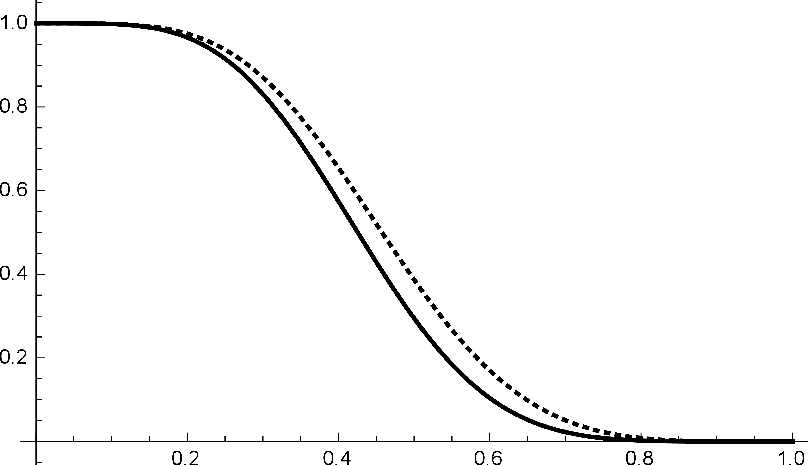
It is routine to check that $\psi(t)$ log-concave.

Figure 1.

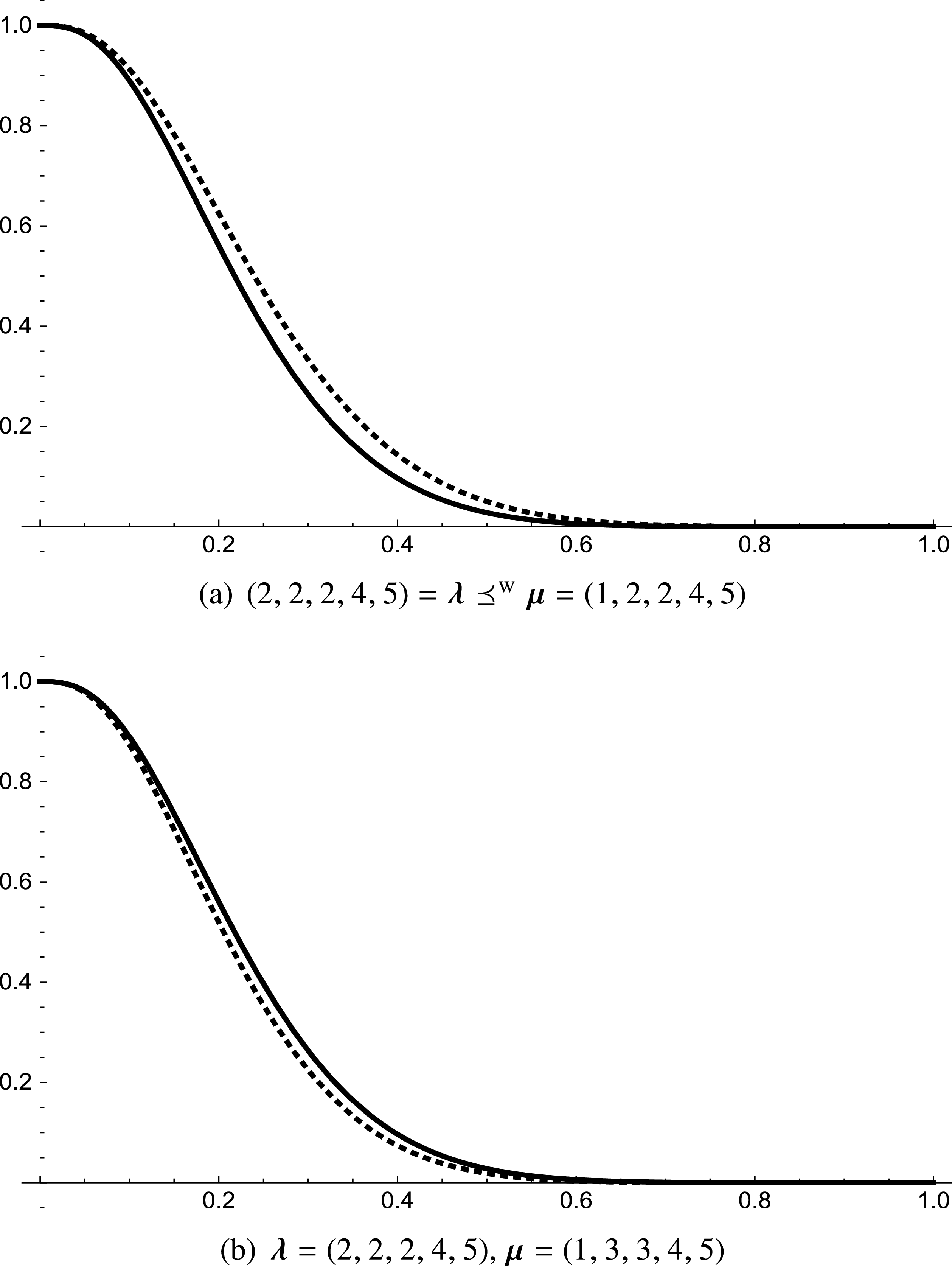
Curves of $\mathbb{P}(X_{3:5}> -\ln(1-s))$ (solid) and $\mathbb{P}(Y_{3:5}> -\ln(1-s))$ (dotted).

1. (i) For $(2, 2, 2, 4, 5)=\boldsymbol{\lambda}\preceq^\text{w}\boldsymbol{\mu}=(1, 2, 2, 4, 5)$ , satisfying the condition in Corollary 3.1, it can be seen in Figure 1(a) that the curve of $\mathbb{P}(X_{3:5}> -\ln(1-s))$ falls under that of $\mathbb{P}(Y_{3:5}> -\ln(1-s))$ over the entire interval (0,1), confirming the usual stochastic order $X_{3:5}\le_{\text{st}}Y_{3:5}$ .

2. (ii) For $(2, 2, 2, 4, 5)=\boldsymbol{\lambda}\preceq_\text{w}\boldsymbol{\mu}=(1, 3, 3, 4, 5)$ , violating the assumption of weak supermajorization in Corollary 3.1, it can be seen in Figure 1(b) that the curve of $\mathbb{P}(X_{3:5}> -\ln(1-s))$ is above that of $\mathbb{P}(Y_{3:5}> -\ln(1-s))$ for all $s\in(0,1)$ , and this indicates the usual stochastic order $X_{3:5}\ge_{\text{st}}Y_{3:5}$ instead.

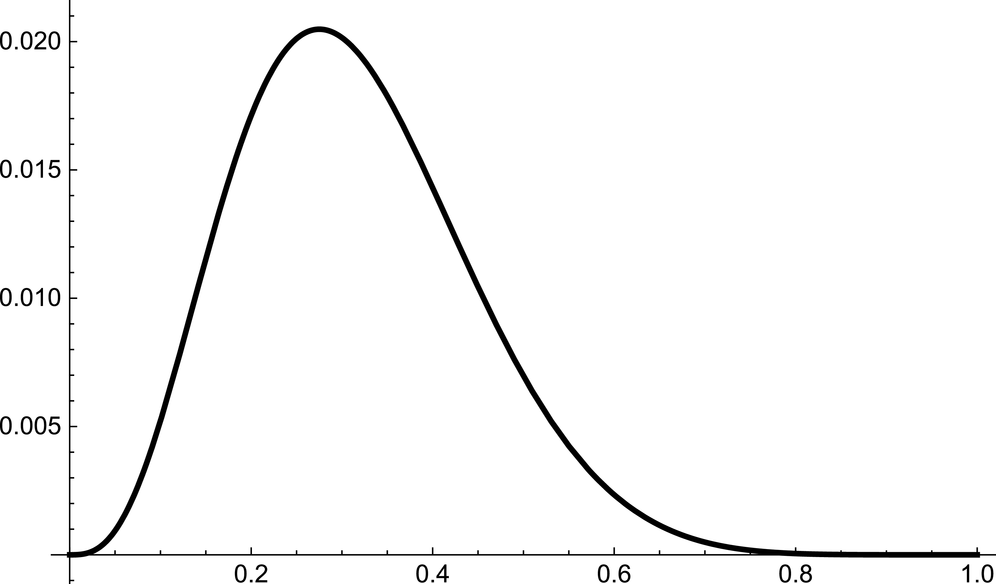
3. (iii) It is easy to check that $(2,2,2,4,6)=\boldsymbol{\lambda}\overset{\mathrm{rm}}{\preceq}\boldsymbol{\mu}=(1,3,3,4,5)$ and none of weak supermajorization, weak submajorization, or p-majorization hold. However, it can be observed in Figure 2 that the difference $\mathbb{P}(X_{3:5}> -\ln(1-s))-\mathbb{P}(Y_{3:5}> -\ln(1-s))$ lies above the horizontal axis on (0,1), and this hints that the weak supermajorization of PHR coefficients is not the necessary factor for the usual stochastic order of the third-smallest order statistics.

Figure 2.

The curve of $\mathbb{P}(X_{3:5}> -\ln(1-s))-\mathbb{P}(Y_{3:5}> -\ln(1-s))$ .

According to Example 3.1(ii), the usual stochastic order in Corollary 3.1 could be reversed if the two frailty parameters are of the weak submajorization order. Also, it should be pointed out that the five-dimensional AMH copula could not have a very small parameter, otherwise the copula would not be a valid member of the Archimedean family. Actually, for most Archimedean copulas with log-concave generator, the higher the dimension, the less negative dependent it is.

4. The third-largest order statistic in the setting of the PRH model

The random variables $X_1,\dots,X_n$ are said to follow the PRH model if $X_i$ has the distribution function $F_i(x)=F^{\lambda_i}(x)$ for any $x\in\mathbb{R}$ and $\lambda_i > 0$ , $i\in\mathcal{I}_n$ , where F is called the baseline distribution function and $\boldsymbol{\lambda}=(\lambda_1,\dots,\lambda_n)$ is the vector of resilience coefficients. For ease of reference, by $\boldsymbol{{X}}\sim \mathrm{PRH}(F,\boldsymbol{\lambda},\psi)$ we denote random variables $X_{1},\dots,X_n$ coupled by the Archimedean copula with generator $\psi$ and following the PRH model with baseline distribution function F and resilience parameter $\boldsymbol{\lambda}$ .

For random variables $\boldsymbol{{X}}\sim\mathrm{PRH}(F,\boldsymbol{\lambda},\psi)$ , we derive the probability distribution function of the third-largest order statistic.

Proposition 4.1. For $\boldsymbol{{X}}\sim\mathrm{PRH}(F,\boldsymbol{\lambda},\psi)$ , the distribution function of $X_{n-2:n}$ is

(4.1) \begin{equation} \mathbb{P}(X_{n-2:n} \le x) = h(F^{\lambda_1}(x),\dots,F^{\lambda_n}(x),\psi) \quad {for\, any\, }\textit{x}\,{ in\, the\, support\, of\, }\textit{F}. \end{equation}

Proof. Note that, for any x in the support of F,

(4.2) \begin{align} \mathbb{P}(X_{n-2:n}\le x) & = \mathbb{P}(X_{n-2:n}\le x,X_{n-1\,:\,n}\le x) + \mathbb{P}(X_{n-2:n}\le x,X_{n-1\,:\,n} > x) \nonumber \\ & = \mathbb{P}(X_{n-1\,:\,n}\le x) + \mathbb{P}(X_{n-2:n}\le x,X_{n-1\,:\,n} > x). \end{align}

According to the discussion in [Reference Fang, Li and Li12, Section 6], we have

(4.3) \begin{equation} \mathbb{P}(X_{n-1\,:\,n}\le x) = \sum_{i=1}^n\mathbb{P}(X_k\le x,k\in\mathcal{I}_n\backslash \{i\}) - (n-1)\mathbb{P}(X_k\le x,k\in\mathcal{I}_n). \end{equation}

Also,

(4.4) \begin{align} \mathbb{P}(X_{n-2:n}\le x,X_{n-1\,:\,n}>x) & = \sum_{1\le i < j\le n}\mathbb{P}(X_i>x,X_j>x,X_k\le x,k\in\mathcal{I}_n\backslash\{i,j\}) \nonumber \\ & = \sum_{1\le i < j\le n}\big[\mathbb{P}(X_k\le x,k\in\mathcal{I}_n\backslash\{i,j\}) - \mathbb{P}(X_k\le x,k\in\mathcal{I}_n\backslash\{i\}) \nonumber \\ & \ \ \qquad\qquad - \mathbb{P}(X_k\le x,k\in\mathcal{I}_n\backslash\{j\}) + \mathbb{P}(X_k\le x,k\in\mathcal{I}_n)\big] \nonumber \\ & = \sum_{1\le i < j\le n}\mathbb{P}(X_k\le x,k\in\mathcal{I}_n\backslash\{i,j\}) \nonumber \\ & \quad - (n-1)\sum_{i=1}^n\mathbb{P}(X_k\le x,k\in\mathcal{I}_n\backslash\{i\}) + \binom{n}{2}\mathbb{P}(X_k\le x,k\in\mathcal{I}_n). \end{align}

Based on (2.5) and (4.2)–(4.4) we have

\begin{align*} \mathbb{P}(X_{n-2:n}\le x) & = \sum_{i=1}^n\Bigg[\mathbb{P}(X_k\le x,k\in\mathcal{I}_n\backslash\{i\}) - (n-1)\mathbb{P}(X_k\le x,k\in\mathcal{I}_n) \\ & \ \ \ \quad\qquad + \sum_{1\le i < j\le n}\mathbb{P}(X_k\le x,k\in\mathcal{I}_n\backslash\{i,j\})\Bigg] \\ & \quad - (n-1)\sum_{i=1}^n\mathbb{P}(X_k\le x,k\in\mathcal{I}_n\backslash\{i\}) + \binom{n}{2}\mathbb{P}(X_k\le x,k\in\mathcal{I}_n) \\ & = \sum_{1\le i < j\le n}\mathbb{P}(X_k\le x,k\in\mathcal{I}_n\backslash\{i,j\}) - (n-2)\sum_{i=1}^n\mathbb{P}(X_k\le x,k\in\mathcal{I}_n\backslash\{i\}) \\ & \quad + \binom{n-1}{2}\mathbb{P}(X_k\le x,k\in\mathcal{I}_n) \\ & = \sum_{1\le i < j\le n}\psi\Bigg(\sum_{k\not\in\{i,j\}}\phi(F^{\lambda_k}(x))\Bigg) - (n-2)\sum_{i=1}^n\psi\Bigg(\sum_{k\neq i}\phi(F^{\lambda_k}(x))\Bigg) \\ & \quad + \binom{n-1}{2}\psi\Bigg(\sum_{k=1}^n\phi(F^{\lambda_k}(x))\Bigg) = h(F^{\lambda_1}(x),\dots,F^{\lambda_n}(x),\psi), \end{align*}

where the function h is defined by (2.5). This yields the desired equation of (4.1).

In the next theorem and corollary we present a characterization and one sufficient condition of the usual stochastic order of the third-largest order statistics from two PRH samples with a common Archimedean copula. Since they can be derived in a very similar manner to those of Theorem 3.1 and Corollary 3.1, respectively, we omit the detailed technical proofs of these two conclusions.

Theorem 4.1. Suppose that $\boldsymbol{{X}}\sim\mathrm{PRH}(F,\boldsymbol{\lambda},\psi)$ and $\boldsymbol{{Y}}\sim\mathrm{PRH}(F,\boldsymbol{\mu},\psi)$ . Then $\boldsymbol{\lambda}\preceq^\text{w}\boldsymbol{\mu}$ implies $X_{n-2:n}\ge_{\text{st}}Y_{n-2:n}$ if and only if

\begin{equation*} \frac{\psi'(\phi(u_r))/u_r}{\psi'(\phi(u_s))/u_s} \le \frac{h_{r}(u_1,\dots,u_n,\psi)}{h_{s}(u_1,\dots,u_n,\psi)} \end{equation*}

for any $u_1,\dots,u_n\in(0,1)$ and $\{r,s\}\subseteq\mathcal{I}_n$ such that $0 < u_s\le u_r<1$ .

Note that the conditions proposed in Theorem 4.1 and Corollary 4.1 are exactly those of Theorem 3.1 and Corollary 3.1, respectively. Since the generator is assumed to be log-concave in both Theorem 3.1 and Theorem 4.1, in what follows we construct one numerical example of the usual stochastic order of the third-largest order statistic in the setting of Theorem 4.1, but the Archimedean copula corresponds to a log-convex generator, and thus the log-concavity is not necessary.

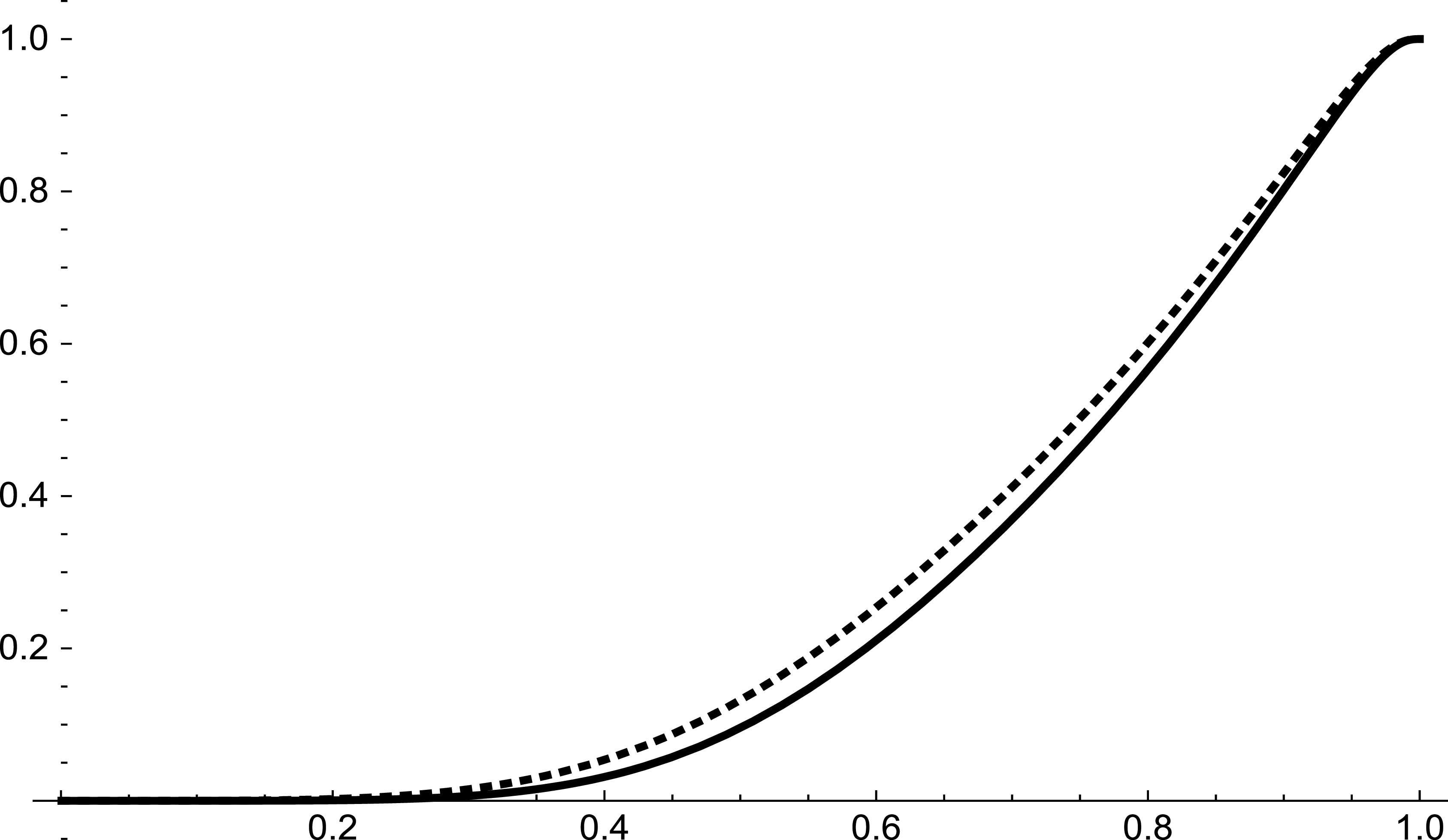
For $\boldsymbol{\lambda}=(2, 2, 2, 4, 5)$ and $\boldsymbol{\mu}=(1, 2, 2, 4, 5)$ , it is routine to check that $\boldsymbol{\lambda}\preceq^\text{w}\boldsymbol{\mu}$ , fulfilling the condition of Theorem 4.1. In Figure 3, we plot the transformed survival curves of $\mathbb{P}(X_{3:5}\le -\ln(1-s))$ and $\mathbb{P}(Y_{3:5}\le -\ln(1-s))$ for $s\in(0,1)$ , respectively. As can be seen, the former curve lies below the latter for all $s\in(0,1)$ . Numerically, this leads to $X_{3:5}\ge_{\text{st}}Y_{3:5}$ , the desired usual stochastic order.

Figure 3.

$\mathbb{P}(X_{3:5}\le -\ln(1-s))$ (solid) and $\mathbb{P}(Y_{3:5}\le -\ln(1-s))$ (dotted).

5. The third-smallest order statistic in the setting of the scale model

The random variables $X_1,\dots,X_n$ are said to follow the scale model if $X_i$ has probability distribution function $F_i(x)=F(\lambda_i x)$ for any $x\ge 0$ and $\lambda_i>0$ , $i\in\mathcal{I}_n$ , where F is the baseline distribution and the parameter $\boldsymbol{\lambda}=(\lambda_1,\dots,\lambda_n)$ is the vector of scale coefficients. Note that $X_i$ has the survival function $\bar{F}_i(x)=\bar{F}(\lambda_i x)$ for any $x\ge 0$ and $\lambda_i>0$ , $i\in\mathcal{I}_n$ . For ease of reference, we denote by $\boldsymbol{{X}}\sim\mathrm{SM}(\bar{F},\boldsymbol{\lambda},\psi)$ random variables $X_1,\dots,X_n$ coupled by the Archimedean survival copula with generator $\psi$ and following the scale model with baseline distribution function F and scale parameter $\boldsymbol{\lambda}$ .

The survival function of the third-smallest order statistic from a scale sample with Archimedean survival copula can be derived in a similar manner to Proposition 3.1.

Proposition 5.1. For $\boldsymbol{{X}}\sim\mathrm{SM}(\bar{F},\boldsymbol{\lambda},\psi)$ , the survival function of $X_{3:n}$ is

\begin{equation*} \mathbb{P}(X_{3:n}>x)=h(\bar{F}(\lambda_1x),\dots,\bar{F}(\lambda_n x),\psi) \quad \mbox{for any $x\ge 0$.} \end{equation*}

Owing to this survival function, we are ready to build the usual stochastic order on the third-smallest order statistic based on a scale sample with Archimedean survival copula.

Theorem 5.1. Suppose that $\boldsymbol{{X}}\sim\mathrm{SM}(\bar{F},\boldsymbol{\lambda},\psi)$ and $\boldsymbol{{Y}}\sim\mathrm{SM}(\bar{F},\boldsymbol{\mu},\psi)$ . Then $\boldsymbol{\lambda}\preceq^\text{w}\boldsymbol{\mu}$ implies $X_{3:n}\le_{\text{st}}Y_{3:n}$ if and only if

(5.1) \begin{equation} \frac{({\partial}/{\partial x_s})\phi(\bar{F}(x_s))}{({\partial}/{\partial x_r})\phi(\bar{F}(x_r))} \le \frac{h_{r}(\bar{F}(x_1),\dots,\bar{F}(x_n),\psi)}{h_{s}(\bar{F}(x_1),\dots,\bar{F}(x_n),\psi)} \end{equation}

for all $x_1,\dots,x_n\ge0$ and any $\{r,s\}\subseteq\mathcal{I}_n$ such that $x_s\ge x_r$ .

Proof. For any x and $s\in\mathcal{I}_n$ , we have

\begin{align*} & \frac{\partial}{\partial\lambda_s}h(\bar{F}(\lambda_1x),\dots,\bar{F}(\lambda_n x),\psi) \\ & \quad= \Bigg[\sum_{\substack{1\le i < j\le n\\ i,j\neq s}}\psi'\Bigg(\sum_{k\not\in\{i,j\}}\phi(\bar{F}(\lambda_kx))\Bigg) - (n-2)\sum_{i\neq s}\psi'\Bigg(\sum_{k\neq i}\phi(\bar{F}(\lambda_kx))\Bigg) \\ & \qquad + \binom{n-1}{2}\psi'\Bigg(\sum_{k=1}^n\phi(\bar{F}(\lambda_kx))\Bigg)\Bigg] \cdot \frac{\partial}{\partial\lambda_s}\phi(\bar{F}(\lambda_sx)) \\ & \quad = h_{s}(\bar{F}(\lambda_1x),\dots,\bar{F}(\lambda_n x),\psi) \cdot \frac{\partial}{\partial\lambda_s}\phi(\bar{F}(\lambda_sx)), \end{align*}

where $h_s$ is defined by (2.6), and hence, for any $x\ge 0$ and $\{r, s\}\subseteq\mathcal{I}_n$ ,

(5.2) \begin{align} & (\lambda_s-\lambda_r)\bigg[ \frac{\partial}{\partial\lambda_s}h(\bar{F}(\lambda_1x),\dots,\bar{F}(\lambda_n x),\psi) - \frac{\partial}{\partial\lambda_r}h(\bar{F}(\lambda_1x),\dots,\bar{F}(\lambda_n x),\psi)\bigg] \nonumber \\ & \quad = (\lambda_s-\lambda_r)\bigg[h_s(\bar{F}(\lambda_1x),\dots,\bar{F}(\lambda_n x),\psi) \cdot \frac{\partial}{\partial\lambda_s}\phi(\bar{F}(\lambda_sx)) \nonumber \\ & \qquad\qquad\qquad\ \ - h_r(\bar{F}(\lambda_1x),\dots,\bar{F}(\lambda_n x),\psi) \cdot \frac{\partial}{\partial\lambda_r}\phi(\bar{F}(\lambda_rx))\bigg]. \end{align}

Similarly to the proof of Theorem 3.1, it can be shown that $h_s(\bar{F}(\lambda_1x),\dots,\bar{F}(\lambda_n x),\psi)\le 0$ for any $x\ge 0$ and $s\in\mathcal{I}_n$ . Let us say that $x_s\ge x_r\ge 0$ . Then (5.2) holds if and only if

\begin{equation*} \frac{({\partial}/{\partial x_s})\phi(\bar{F}(x_s))}{({\partial}/{\partial x_r})\phi(\bar{F}(x_r))} \le \frac{h_{r}(\bar{F}(x_1),\dots,\bar{F}(x_n),\psi)}{h_{s}(\bar{F}(x_1),\dots,\bar{F}(x_n),\psi)} \end{equation*}

for any $x_1,\dots,x_n\ge0$ and $\{r,s\}\subseteq\mathcal{I}_n$ . This is exactly (5.1), the desired result.

Unlike the characterizations of Theorems 3.1 and 4.1, the necessary and sufficient condition of (5.1) is a compound of the baseline survival function and the generator associated with the survival copula. For ease of verification, we next present two simple sufficient conditions.

Proof. Similarly to the proof of Corollary 3.1, it can be shown that

(5.3) \begin{equation} \frac{h_{r}(\bar{F}(x_1),\dots,\bar{F}(x_n),\psi)}{h_{s}(\bar{F}(x_1),\dots,\bar{F}(x_n),\psi)}\ge1 \end{equation}

for any $x_1,\dots,x_n\ge0$ and $\{r,s\}\subseteq\mathcal{I}_n$ such that $x_s\ge x_r$ . On the other hand, it is clear that $\phi(\bar{F}(x))$ is increasing in x. If $\phi(\bar{F}(x))$ is concave in x, then

\begin{equation*} \frac{\partial}{\partial x_r}\phi(\bar{F}(x_r)) \ge \frac{\partial}{\partial x_s}\phi(\bar{F}(x_s))\ge0 \end{equation*}

for any $\{r,s\}\subseteq\mathcal{I}_n$ such that $x_s\ge x_r\ge0$ , and hence

(5.4) \begin{equation} \frac{({\partial}/{\partial x_s})\phi(\bar{F}(x_s))}{({\partial}/{\partial x_r})\phi(\bar{F}(x_r))}\le 1. \end{equation}

Clearly, (5.3) along with (5.4) yields the sufficient and necessary condition of (5.1), and thus it follows from Theorem 5.1 that $\boldsymbol{\lambda}\preceq^\text{w}\boldsymbol{\mu}$ implies $X_{3:n}\le_{\text{st}}Y_{3:n}$ .

Proof. Clearly,

(5.5) \begin{equation} \frac{\partial}{\partial x}\phi(\bar{F}(x)) = -\frac{f(x)}{\psi'(\phi(\bar{F}(x)))} = -\frac{f(x)}{\bar{F}(x)} \cdot \frac{\psi(\phi(\bar{F}(x)))}{\psi'(\phi(\bar{F}(x)))}. \end{equation}

Since $\psi$ is log-concave, $\psi/\psi'$ is increasing and hence

\begin{equation*}\frac{\psi(\phi(\bar{F}(x)))}{\psi'(\phi(\bar{F}(x)))}\end{equation*}

is non-positive and increasing in x. On the other hand, owing to F with DHR, $f(x)/\bar{F}(x)$ is decreasing in x. In combination, we conclude that $({\partial}/{\partial x})\phi(\bar{F}(x))$ of (5.5) is decreasing in x. That is, $\phi(\bar{F}(x))$ is concave in x. Thus, owing to Corollary 5.1, $\boldsymbol{\lambda}\preceq^\text{w}\boldsymbol{\mu}$ implies $X_{3:n}\le_{\text{st}}Y_{3:n}$ .

Here, we employ two examples to demonstrate that, along with a DHR (IHR) baseline survival function $\bar{F}$ , the log-convex (log-concave) generator $\psi(t)$ may also yield the concavity of $\phi(\bar{F}(x))$ , the sufficient condition of Corollary 5.1.

Example 5.2. (Gumbel–Barnett copula.) Consider the survival copula with generator (2.4), i.e. 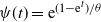$\psi(t)={\mathrm{e}}^{(1-{\mathrm{e}}^t)/\theta}$ for $t\ge 0$ , and the baseline survival function

\begin{equation*} \bar{F}(x) = \begin{cases} {\mathrm{e}}^{-x}, & 0 < x < 1, \\ {\mathrm{e}}^{-1.1x+0.1}, & x\ge1, \end{cases} \end{equation*}

where $\theta\in[0,1]$ . Clearly, $\bar{F}$ is IHR and $\psi$ is log-concave. Also, we have

\begin{equation*} \phi(\bar{F}(x)) = \begin{cases} \ln(1+\theta x), & 0 < x < 1, \\ \ln(1-0.1\theta+1.1\theta x), & x\ge1. \end{cases} \end{equation*}

Note that

\begin{equation*} \frac{\partial^2}{\partial x^2}\phi(\bar{F}(x)) = \begin{cases} -\theta^2(1+\theta x)^{-2}, & 0 < x < 1, \\ -1.21\theta^2(1-0.1\theta+1.1\theta x)^{-2}, & x\ge1, \end{cases} \end{equation*}

which is non-positive. That is, $\phi(\bar{F}(x))$ is concave in x.

Also, we present one numerical example to demonstrate that neither of the two sufficient conditions of Corollaries 5.1 and 5.2 is necessary.

Example 5.3. (AMH copula.) Suppose two five-dimensional samples $\boldsymbol{{X}}\sim \mathrm{SM}(\bar{F},\boldsymbol{\lambda},\psi)$ and $\boldsymbol{{Y}}\sim \mathrm{SM}(\bar{F},\boldsymbol{\mu},\psi)$ with baseline distribution function $\bar F(t)={\mathrm{e}}^{-(t/2)^{1.5}}$ for all $t\ge 0$ and AMH copula corresponding to log-concave generator

\begin{equation*}\psi(t)=\frac{1.042}{{\mathrm{e}}^t+0.042} \quad \mbox{for all $t\ge 0$.}\end{equation*}

The baseline distribution can be easily verified to be of increasing hazard rate instead, and this negates the assumption of DHR. In addition, it can also be easily checked that $\phi(\bar{F}(x))$ is convex in x, violating the sufficient condition of Corollary 5.1.

Note that $\boldsymbol{\lambda}=(2, 2, 2, 4, 5)\preceq^\text{w}(1, 2, 2, 4, 5)=\boldsymbol{\mu}$ fulfills the condition of Corollary 5.2. Figure 4 shows two curves, $\mathbb{P}(X_{3:5}> -\ln(1-s))$ and $\mathbb{P}(Y_{3:5}> -\ln(1-s))$ ; it can be observed that the former falls below the latter over the whole interval (0, 1), and this justifies $X_{3:5}\le_{\text{st}}Y_{3:5}$ , as is claimed in Corollary 5.2.

Figure 4.

$\mathbb{P}(X_{3:5}>-\ln(1-s))$ (solid) and $\mathbb{P}(Y_{3:5}> -\ln(1-s))$ (dotted).

6. Some simulation results

Nadeb et al. [Reference Nadeb, Torabi and Dolati33] studied the usual stochastic order of extreme order statistics from the semi-parameter models $\bar{F}(x,\lambda)$ and $F(x,\lambda)$ with Archimedean copulas and survival copulas, respectively. Since the PHR model $\bar F^{\lambda}(x)$ , PRH model $F^{\lambda}(x)$ , and scale model $F(\lambda x)$ are special cases of such semi-parameter models, it is worth clarifying the difference and similarity between the sufficient condition of the present study and that of [Reference Nadeb, Torabi and Dolati33]. All Archimedean copulas in this study are assumed to have a log-concave generator corresponding to negative dependence, while in [Reference Nadeb, Torabi and Dolati33] the generators are supposed to be log-convex defining positive dependence. On the other hand, the PHR model $\bar{F}^{\lambda}(x)$ of Corollary 3.1 is decreasing and log-concave in $\lambda$ , consistent with the condition of [Reference Nadeb, Torabi and Dolati33, Theorem 3.1], and the PRH model $F^{\lambda}(x)$ of Corollary 4.1 is decreasing and log-concave in $\lambda$ , consistent with the condition of [Reference Nadeb, Torabi and Dolati33, Theorem 3.2]. As for the scale model $F(\lambda x)$ with F having DHR in Corollary 5.2, it can be verified that $F(\lambda x)$ is increasing and log-concave in $\lambda$ , fulfilling the condition of [Reference Nadeb, Torabi and Dolati33, Theorem 3.2].

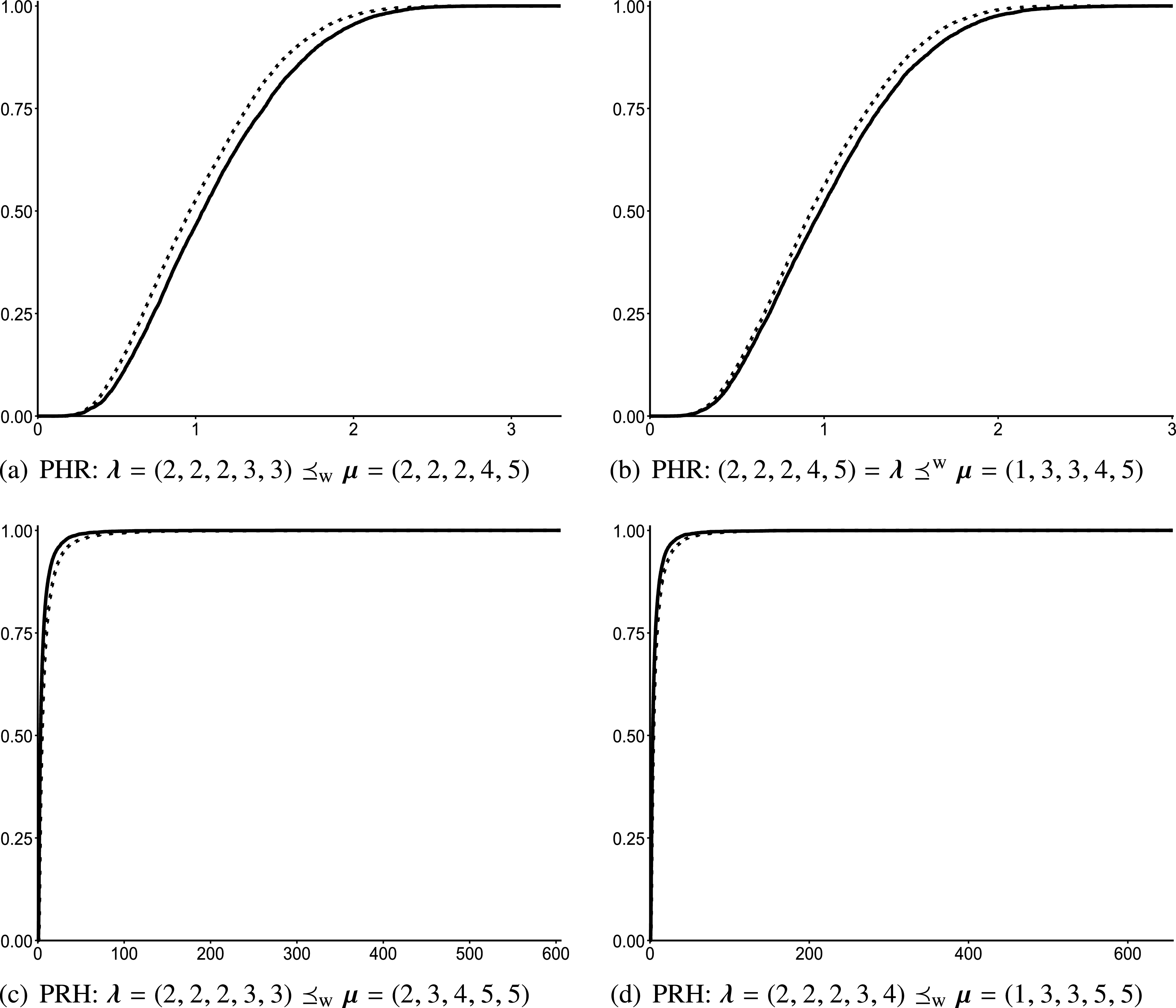
The assumptions and results are quite different between these two studies. In this section, we further illustrate our findings and probe the usual stochastic order of the third order statistic under the condition of [Reference Nadeb, Torabi and Dolati33] using several Monte Carlo simulations. Specifically, for different five-dimensional distributions following the PHR, PRH, and SM models, we generate random samples of $n=10\,000$ observations $\boldsymbol{{t}}_{i}=(t_{i,1},t_{i,2},t_{i,3},t_{i,5},t_{i,5})$ , $i=1,\dots,n$ , collect third order statistics $t_{3\,:\,5,1},\dots,t_{3\,:\,5,n}$ , and then based on them we plot the empirical distribution function (EDF) to check if one curve lies above another.

Although standard Archimedean copulas with log-convex generators (e.g. Clayton, Gumbel) are well supported in R packages like copula, those with log-concave generators are less common and often lack closed-form Laplace inverses. For such cases, we can implement numerical inversion of the Laplace transform or use conditional sampling with numerical root-finding. As an alternative, a Bayesian Markov chain Monte Carlo approach via rstan can be employed, though it is computationally inefficient for pure random sampling. In our simulation, we use rstan only for log-concave cases where standard numerical methods are impractical, and the copula package otherwise.

Example 6.1. (AMH copula.) In the context of Example 3.1(i), set the log-concave generator $\psi(t)={1.042}/({{\mathrm{e}}^t+0.042})$ for $t\ge 0$ . Clearly, $\boldsymbol{\lambda}=(2, 2, 2, 4, 5)\preceq^\text{w}(1, 2, 2, 4, 5)=\boldsymbol{\mu}$ , and it can be checked that $\boldsymbol{\lambda}^*=(1/3, 3/8, 4/9, 9/8, 6)$ and $\boldsymbol{\mu}^*=(1/4, 4/7, 9/4, 9/4, 9/2)$ are not ordered by any one of weak supermajorization, weak submajorization, p-majorization, or reciprocal majorization.

First, we consider $\boldsymbol{{X}}\sim \textrm{PHR}(\bar{F},\boldsymbol{\lambda},\psi)$ and $\boldsymbol{{Y}}\sim \textrm{PHR}(\bar{F},\boldsymbol{\mu},\psi)$ with Weibull baseline survival function $\bar F(t)={\mathrm{e}}^{-(t/2)^2}$ for all $t\ge 0$ . Figure 5(a) plots the EDFs of $X_{3:5}$ and $Y_{3:5}$ with $\boldsymbol{\lambda}\preceq^\text{w}\boldsymbol{\mu}$ . As can be seen, $X_{3:5}$ does have a larger EDF, confirming the result of Corollary 3.1. In Figure 5(b), for $\boldsymbol{\lambda}^*$ and $\boldsymbol{\mu}^*$ $X_{3:5}$ tends to have a smaller EDF, negating $X_{3:5}\le_{\text{st}}Y_{3:5}$ .

Figure 5.

Empirical distribution functions of $X_{3:5}$ (solid) and $Y_{3:5}$ (dotted).

Second, we examine $\boldsymbol{{X}}\sim \textrm{PRH}(F,\boldsymbol{\lambda},\psi)$ and $\boldsymbol{{Y}}\sim \textrm{PRH}(F,\boldsymbol{\mu},\psi)$ with baseline distribution function $F(t)=1-{\mathrm{e}}^{-t}$ for $t\ge 0$ . As can be seen in Figure 5(c), with $\boldsymbol{\lambda}\preceq^\text{w}\boldsymbol{\mu}$ $X_{3:5}$ has a smaller EDF than $Y_{3:5}$ , and this confirms Corollary 4.1. However, in Figure 5(d), corresponding to $\boldsymbol{\lambda}^*$ and $\boldsymbol{\mu}^*$ , $X_{3:5}$ tends to have a larger EDF, and this negates the result of Corollary 4.1.

Last, for $\boldsymbol{{X}}\sim \textrm{SM}(\bar F,\boldsymbol{\lambda},\psi)$ and $\boldsymbol{{Y}}\sim \textrm{SM}(\bar F,\boldsymbol{\mu},\psi)$ with baseline survival function $\bar F(t)={\mathrm{e}}^{-(t/2)^{0.5}}$ for $t\ge 0$ having DHR, in Figure 5(e) with $\boldsymbol{\lambda}\preceq^\text{w}\boldsymbol{\mu}$ it is observed that $X_{3:5}$ does have a larger EDF and hence confirms the result of Corollary 5.2, whereas in Figure 5(f) with $\boldsymbol{\lambda}^*$ and $\boldsymbol{\mu}^*$ , $X_{3:5}$ tends to have a smaller EDF than $Y_{3:5}$ , reversing the ordering result of Corollary 5.2.

Example 6.2. (Frank copula.) In the setting of Example 4.1, let us consider the log-convex generator $\psi(t)=-\ln[{\mathrm{e}}^{-t}({\mathrm{e}}^{-3}-1)+1]/3$ for $t\ge 0$ .

For $\boldsymbol{{X}}\sim \textrm{PHR}(\bar{F},\boldsymbol{\lambda},\psi)$ and $\boldsymbol{{Y}}\sim \textrm{PHR}(\bar{F},\boldsymbol{\mu},\psi)$ with baseline survival function $\bar F(t)={\mathrm{e}}^{-t}$ for all $t\ge 0$ and $\boldsymbol{\lambda}=(2, 2, 2, 3, 3)\preceq_\text{w}(2, 2, 2, 4, 5)=\boldsymbol{\mu}$ , both copula and PHR model satisfy the condition of [Reference Nadeb, Torabi and Dolati33, Theorem 3.1]. In Figure 6(a) we observe that $X_{3:5}$ tends to have a smaller EDF, conforming $X_{3:5}\ge_{\text{st}}Y_{3:5}$ of [Reference Nadeb, Torabi and Dolati33, Theorem 3.1]. As for Figure 6(b), with $\boldsymbol{\lambda}=(2, 2, 2, 4, 5)\preceq^\text{w}\boldsymbol{\mu}=(1, 3, 3, 4, 5)$ $X_{3:5}$ tends to have a larger EDF than $Y_{3:5}$ , indicating that $X_{3:5}\ge_{\text{st}}Y_{3:5}$ even without the condition of [Reference Nadeb, Torabi and Dolati33, Theorem 3.1].

Corresponding to $\boldsymbol{{X}}\sim \textrm{PRH}(F,\boldsymbol{\lambda},\psi)$ and $\boldsymbol{{Y}}\sim \textrm{PRH}(F,\boldsymbol{\mu},\psi)$ with baseline distribution function $F(t)={\mathrm{e}}^{-1/t}$ for $t\ge 0$ , in Figure 6(c) with $\boldsymbol{\lambda}=(2, 2, 2, 3, 3)\preceq_\text{w}(2, 2, 2, 4, 5)=\boldsymbol{\mu}$ , $X_{3:5}$ is observed to have a larger EDF, implying that $X_{3:5}\le_{\text{st}}Y_{3:5}$ in the context of [Reference Nadeb, Torabi and Dolati33, Theorem 3.2], and in Figure 6(d) with $\boldsymbol{\lambda}=(2, 2, 2, 3, 4)\preceq^\text{w}(1, 3, 3, 5, 5)=\boldsymbol{\mu}$ , $X_{3:5}$ again seems to have a larger EDF than $Y_{3:5}$ , hinting that $X_{3:5}\le_{\text{st}}Y_{3:5}$ even though the condition of [Reference Nadeb, Torabi and Dolati33, Theorem 3.2] is not fulfilled.

Figure 6.

Empirical distribution functions of $X_{3:5}$ (solid) and $Y_{3:5}$ (dotted).

7. Three related applications

In this section we propose some interesting applications of the three main conclusions presented in the previous sections. Due to our background, we pay attention to reliability theory, multiple-outlier models, and the third-price auction.

7.1. Reliability of voting systems with dependent component lifetimes

In the context of engineering reliability, based on components with lifetimes $X_1,\dots,X_n$ , the third-smallest order statistic $X_{3:n}$ characterizes the lifetime of the $(n-2)$ -out-of-n:G system, which works if at least $n-2$ of all n components function properly. As a dual, the third-largest order statistic $X_{n-2:n}$ defines the lifetime of the three-out-of-n:G system, which works if at least three of all n components operate properly. As the building block of coherent systems, voting systems have received much attention in the past several decades. For a comprehensive exposition of voting systems with components having i.i.d. lifetimes, we refer readers to [Reference Kuo and Zuo20, Chapter 7].

According to Corollary 3.1, for components having lifetimes following the PHR model and linked by an Archimedean survival copula associated with a log-concave generator, a less weakly supermajorized vector of PHR coefficients leads to a stochastically smaller lifetime for the $(n-2)$ -out-of-n:G system, and thus, with a resource constraint in terms of a fixed sum of PHR coefficients, the reliability engineer should pursue the design with a more majorized vector of PHR coefficients. Owing to their importance and popularity in engineering reliability, Weibull distributions are constantly discussed in the context of parallel and series structures of heterogeneous components, and several ordering results have been developed in the literature; see, for example, [Reference Li and Li22, Reference Torrado39, Reference Torrado and Kochar41].

Assume that the component lifetime $X_i$ has Weibull distribution $\bar{F}_i(x)=\exp\{-\alpha_ix^\lambda\}$ , $\lambda>0,x>0$ , $\alpha_i>0$ , $i=1,\dots,n$ , and that $(X_1,\dots,X_n)$ are linked by an AMH survival copula associated with generator $\psi(t)=(1-\theta)/({\mathrm{e}}^{t}-\theta)$ for all $t\ge 0$ , which is log-concave on $[0,\infty)$ for $\theta\in(\theta_n,0)$ , where $\theta_n\in(\!-1,0)$ is some constant related to the number of components. Then $(X_1,\dots,X_n)$ has the survival function

\begin{equation*}\bar{H}_{\mathrm{w}}(\boldsymbol{{x}},\theta,\lambda,\boldsymbol{\alpha}) =\frac{\prod_{i=1}^{n}\exp\{-\alpha_ix_i^\lambda\}}{1-\theta\prod_{i=1}^{n}(1-\exp\{-\alpha_ix_i^\lambda\})}\quad\mbox{for any $x_i\ge 0$, $i=1,\dots,n$.}\end{equation*}

Note that $X_1,\dots,X_n$ follow the PHR model with baseline survival function $\bar{F}(x)={\mathrm{e}}^{-x^{\lambda}}$ and the vector of proportional coefficients $(\alpha_1,\dots,\alpha_n)\stackrel{\textrm{m}}{\succeq}(\bar\alpha,\dots,\bar\alpha)$ with $\bar\alpha=(\alpha_1+\dots+\alpha_n)/n$ . By Corollary 3.1 we have the following lower bound of the system reliability:

\begin{equation*}\mathbb{P}(X_{3:n}>x)\ge\mathbb{P}(Y_{3:n}>x) \quad\mbox{for any $x\ge 0$,}\end{equation*}

where $Y_{3:n}$ is based on $(Y_1,\dots,Y_n)$ with survival function $\bar{H}_{\mathrm{w}}(\boldsymbol{{x}},\theta,\lambda,\bar\alpha\mathbf{1}_n)$ , and then the lower bound $\mathbb{P}(Y_{3:n}>x)$ can be obtained from (3.1) through (2.5).

On the other hand, as per Corollary 4.1, in the context of component lifetimes following the PRH model and linked by an Archimedean copula with a log-concave generator, a less weakly supermajorized vector of proportional coefficients corresponds to a stochastically larger lifetime for the three-out-of-n:G system. Thus, with the resource constraint in terms of a fixed sum of proportional coefficients, reliability engineers should pursue the system design with the vector of proportional coefficients less majorized instead.

Consider the component lifetime $X_i$ with Fréchet distribution function $G_i(x)=\exp\{-\beta_ix^{-\alpha}\}$ for $\alpha>0$ , $x\ge 0$ , $\beta_i>0$ , $i=1,\dots,n$ , and assume that $(X_1,\dots,X_n)$ are linked by an AMH copula again. Then $(X_1,\dots,X_n)$ has the multivariate Fréchet distribution

\begin{equation*}H_{\mathrm{f}}(\boldsymbol{{x}},\theta,\alpha,\boldsymbol{\beta}) =\frac{\prod_{i=1}^{n}\exp\big\{-\beta_ix_i^{-\alpha}\big\}}{1-\theta\prod_{i=1}^{n}\big(1-\exp\big\{-\beta_ix_i^{-\alpha}\big\}\big)}\quad \mbox{for any $x_i \gt 0$, $i=1,\dots,n$}.\end{equation*}

In accordance with Corollary 4.1, we conclude that $\mathbb{P}(X_{n-2:n}>x)\le\mathbb{P}(Y_{n-2:n}>x)$ for any $x\ge 0$ , where $Y_{n-2:n}$ is based on $(Y_1,\dots,Y_n)$ with distribution function $H_{\mathrm{f}}(\boldsymbol{{x}},\theta,\alpha, \bar\beta\mathbf{1}_n)$ ; then, based on (4.1) and hence (2.6), we can derive $\mathbb{P}(Y_{n-2:n}>x)$ , the upper bound of the system reliability.

7.2. Skewness of multiple-outlier models

With more than one different scale coefficients as impurities, multiple-outlier models have been widely used to study the robustness of different estimators of model parameters. It is believed that the outliers make the sample more skewed and hence the sample extremes reveal stochastic orders in some sense. In the literature, much research has been devoted to stochastic comparison on the single- and multiple-outlier models in the past two decades. For references on models of independent observations, see [Reference Amini-Seresht, Qiao, Zhang and Zhao1, Reference Khaledi and Kochar17, Reference Kochar and Xu19, Reference Torrado40, Reference Xu, Li, Zhao and Li43–Reference Zhao and Balakrishnan45]. Also, it should be remarked here that [Reference Navarro, Torrado and Águila34] further studied stochastic comparison on the largest order statistic from multiple-outlier models of random variables equipped with a general copula.

Denote by $\textrm{SM}(\bar{F},\boldsymbol{\lambda},\psi)$ the scale model corresponding to baseline survival function F, vector of coefficients $\boldsymbol{\lambda}$ , and an Archimedean copula associated with generator $\psi$ . Recently, in the context of $\boldsymbol{{X}}\sim\textrm{SM}(\bar{F},(\lambda_1\mathbf{1}_{n_1},\lambda_2\mathbf{1}_{n_2}),\psi)$ with $\lambda_2\ge\lambda_1\ge 0$ and $\boldsymbol{{Y}}\sim\textrm{SM}(\bar{F},(\mu^{}_1\mathbf{1}_{n_1},\mu^{}_2\mathbf{1}_{n_2}),\psi)$ with $\mu^{}_2\ge\mu^{}_1\ge 0$ , [Reference Das and Kayal9, Corollary 1(ii)] showed that

\begin{equation*}(\lambda_1\mathbf{1}_{n_1},\lambda_2\mathbf{1}_{n_2})\preceq^\text{w}(\mu^{}_1\mathbf{1}_{n_1},\mu^{}_2\mathbf{1}_{n_2})\quad\implies\quad X_{n:n}\le_{\text{st}}Y_{n:n}\end{equation*}

whenever $\psi$ is log-convex and F is DRHR. In fact, this conclusion follows as a direct consequence of [Reference Li, Fang and Li21, Theorem 4.4(ii)].

Now let us consider the multiple-outlier models of $\boldsymbol{{X}}\sim\textrm{SM}(\bar{F},(\lambda_1\mathbf{1}_{n_1},\lambda_2\mathbf{1}_{n_2}),\psi)$ with $\lambda_2\ge\lambda_1\ge 0$ and $\boldsymbol{{Y}}\sim\textrm{SM}(\bar{F},(\mu^{}_1\mathbf{1}_{n_1},\mu^{}_2\mathbf{1}_{n_2}),\psi)$ with $\mu^{}_2\ge\mu^{}_1\ge 0$ . As an immediate application of [Reference Li, Fang and Li21, Theorems 4.2 and 4.3], we conclude that

\begin{equation*}(\lambda_1\mathbf{1}_{n_1},\lambda_2\mathbf{1}_{n_2})\preceq^\text{w}(\mu^{}_1\mathbf{1}_{n_1},\mu^{}_2\mathbf{1}_{n_2})\quad \implies\quad X_{i:n}\le_{\text{st}}Y_{i:n},\quad i=1,2,\end{equation*}

whenever $\psi$ is log-concave and F is DHR. Also, in accordance with Corollary 5.2, we further conclude that

\begin{equation*}(\lambda_1\mathbf{1}_{n_1},\lambda_2\mathbf{1}_{n_2})\preceq^\text{w}(\mu^{}_1\mathbf{1}_{n_1},\mu^{}_2\mathbf{1}_{n_2})\quad\implies\quad X_{3:n}\le_{\text{st}}Y_{3:n}\end{equation*}

whenever $\psi$ is log-concave and F is DHR.

8. Concluding remarks

For random variables following PHR/scale (PRH) models and linked by an Archimedean survival copula and distributional copula, we developed a necessary and sufficient condition for the usual stochastic order of the third-smallest and third-largest order statistics, respectively. Some related sufficient conditions are also presented for technical convenience. As essential extensions of the ordering results on the second-smallest (-largest) order statistics in the literature, the present ordering results are found to be of interest in applications in areas related to reliability theory, multiple outlier models, and third-price auction.

Inspired by these findings, we look forward to conducting further research in this direction. For example, in parallel with [Reference Li and Fang26, Theorem 4.1], it is of interest to investigate how the degree of log-concavity of the generator plays a part in impacting the usual stochastic order of the third-order statistics along with the majorization of proportional coefficients. Also, readers may wonder if, for $k>3$ , the present ordering results can be further extended to the kth-smallest and -largest order statistics in similar contexts. Here is one possible road map to the corresponding results: in view of

\begin{align*} \mathbb{P}(X_{k+1\,:\,n}>x) & = \mathbb{P}(X_{k+1\,:\,n}>x,X_{k:n}>x) + \mathbb{P}(X_{k+1\,:\,n}>x,X_{k:n}\le x) \\ & = \mathbb{P}(X_{k:n}>x) + \mathbb{P}(X_{k+1\,:\,n}>x,X_{k:n}\le x),\end{align*}

we may check the feasibility of building the monotonicity of $\mathbb{P}(X_{k+1\,:\,n}>x,X_{k:n}\le x)$ and then come up with a proof by induction. Of course, researchers may examine the characterization of the hazard rate order and the reversed hazard rate order on the third-order statistics in this context. In addition, since the PRH model $F^{\lambda}(x)$ , scale model $F(\lambda x)$ , and PHR model $\bar F^{\lambda}(x)$ all are special cases of the semi-parameter models $F(x,\lambda)$ and $\bar{F}(x,\lambda)$ , respectively, it is a matter of considerable interest to investigate the usual stochastic order of both the second- and third-smallest or -largest order statistics along the lines of [Reference Nadeb, Torabi and Dolati33]. All such studies are of both theoretical and practical value and therefore merit further exploration in the future.