1. Introduction
Shape oscillations of drops have been the subject of scientific investigations for over 140 years, for fundamental interest and for their relevance for transport processes across the drop surface. Departure of the drop from the spherical equilibrium state makes the drop surface area increase. Furthermore, the motion of the surface and the bulk of the drop induces gradients of velocity, temperature and species mass concentration, influencing the transport of momentum, heat and mass. In the appendix to his paper on the capillary phenomena of jets, Rayleigh (Reference Rayleigh1879) presented a linear analysis of shape oscillations of an inviscid drop in a vacuum around a spherical equilibrium state. One result is the equation for the angular frequency of oscillation of the drop deformed according to a mode  $m$ assuming natural values
 $m=2,3,4,\ldots$ which count the number of lobes on the drop surface. Lamb generalised Rayleigh's result by accounting for the drop viscosity and the density of the ambient medium (Lamb Reference Lamb1881, Reference Lamb1932). He predicted the threshold Ohnesorge number
 $Oh = \mu / (\sigma a \rho )^{1/2}$ of the drop for the onset of aperiodic motion.
Chandrasekhar (Reference Chandrasekhar1959) presented a normal-mode analysis of small oscillations of a viscous self-gravitating globe in a vacuum. In this work, the velocity field and stress tensor in the oscillating globe were determined as solutions of the linearised Navier–Stokes equations with account for gravity. The characteristic equation of the globe was developed, which determines the complex angular oscillation frequency. Later, Reid (Reference Reid1960) showed that the results of such an analysis are the same when the restoring forces producing the tendency to the spherical form are due to surface tension instead of self-gravitation. A further generalisation of the analysis of linear drop shape oscillations is due to Miller & Scriven (Reference Miller and Scriven1968), who accounted for both the viscous and the inertial influences from an ambient medium hosting a viscous oscillating drop. Analysing drop shape oscillations as the solution of an initial-value problem, Prosperetti (Reference Prosperetti1980a) showed that analyses of linear drop oscillations by the normal-mode approach may miss the fact that, in a range of Ohnesorge numbers, oscillations starting in an aperiodic manner may turn into periodic with ongoing time. The most important results, that the papers cited here highlight, are the angular frequency and damping rate of the oscillations, as well as the time-dependent shapes of the oscillating drops.
The first computational investigations of nonlinear drop shape oscillations with large amplitudes are due to Foote (Reference Foote1973) and Alonso (Reference Alonso1974). Both Foote and Alonso used the marker-and-cell finite-difference technique for numerically simulating the time-dependent free-surface flows with weak influence from the liquid viscosity. Foote (Reference Foote1973) predicted the oscillation frequency of drops which were initially deformed and at rest. The initial drop shapes were either oblate spheroids or given by a Legendre polynomial of a certain degree  $m$. It was shown that the oscillation frequency decreased with increasing aspect ratio of the slightly viscous drop. Alonso (Reference Alonso1974) simulated oscillations of atomic nuclei and drops initially at rest and prolate deformed according to a Legendre polynomial. Initially, large deformations and electrical charges of the oscillating drops were addressed. Results consist in surface area, kinetic and Coulomb energies as functions of time during the oscillations. Both fission in large-amplitude oscillations and merging after collisions are addressed. First experimental studies of large-amplitude shape oscillations of drops in an immiscible host liquid and of levitated free liquid drops in air are due to Trinh & Wang (Reference Trinh and Wang1982), who showed the frequency decrease with increasing drop deformation and an asymmetry of the times spent in the prolate and oblate shapes of the two-lobed oscillation mode.
Motivated by these numerical and experimental studies, Tsamopoulos & Brown (Reference Tsamopoulos and Brown1983) investigated nonlinear oscillations of inviscid drops and bubbles for the deformation modes  $m = 2, 3$ and
 $4$ theoretically by means of weakly nonlinear analysis, using the Poincaré–Lindstedt expansion of the drop shape, the velocity potential and the oscillation frequency. Similar to Foote (Reference Foote1973) and Alonso (Reference Alonso1974), the drop shapes found deviated from the linear results, and angular frequencies decreased with increasing oscillation amplitude (for a maximum prolate aspect ratio of the two-lobed shape of 1.4 by approximately 5 %). With increasing oscillation amplitude, the motion also gradually loses the sinusoidal dependency on time, giving rise to an asymmetry of times during one oscillation period spent in the prolate and the oblate states of the two-lobed oscillation mode. The resonant oscillations theoretically investigated by Tsamopoulos & Brown (Reference Tsamopoulos and Brown1984) for inviscid drops led to predictions of charged-drop resonance for different modes of drop deformation. The internal resonance between different modes of deformation in inviscid three-dimensional nonlinear oscillations was the topic of Natarajan & Brown (Reference Natarajan and Brown1987). Lundgren & Mansour (Reference Lundgren and Mansour1988) developed a numerical boundary-integral method to investigate mode coupling in large-amplitude oscillations of large axially symmetric liquid drops including the effects of small viscosity. This work gave insight into instabilities due to large drop surface deformations and resonant energy transfer to higher-order frequencies. Both experimentally and theoretically, Becker, Hiller & Kowalewski (Reference Becker, Hiller and Kowalewski1991) found that nonlinear motion in oscillating drops arises when the amplitude of the fundamental mode exceeds approximately 10 % of the undeformed drop radius. They proposed an inviscid theoretical model applicable for determining the surface tension from large-amplitude oscillations of low-viscosity droplets. Numerical investigations of medium- and large-amplitude oscillations of inviscid and viscous drops are due to Patzek et al. (Reference Patzek, Benner, Basaran and Scriven1991) and Basaran (Reference Basaran1992), respectively. The former work detected mode coupling by a Fourier spectral analysis of the deformed drop surface and related the frequency decrease to higher harmonics. The latter work by Basaran (Reference Basaran1992) showed that mode coupling in drops of finite viscosity was far more intense than with only an infinitesimal amount of viscosity. Both works showed an increase in the difference of times spent in the prolate and oblate states and a frequency decrease with increasing drop deformation, in agreement with earlier results from the literature. The drop spends more time in the prolate than in the oblate state. Furthermore, it was found that the initial state of the drop (deformed and at rest, or spherical and disturbed by some pressure impulse) had an influence on the mode coupling and time asymmetry found in the oscillatory motion, while the frequency decrease was widely unaffected by the initial conditions. Viscous drops spend less time in the prolate form than inviscid drops when released from a steady acoustic drive, but more time in the prolate form than inviscid drops when released from an initial static deformed state (Patzek et al. Reference Patzek, Benner, Basaran and Scriven1991). Meradji et al. (Reference Meradji, Lyubimova, Lyubimov and Roux2001) demonstrated that the results of Lundgren & Mansour (Reference Lundgren and Mansour1988), Patzek et al. (Reference Patzek, Benner, Basaran and Scriven1991) and Basaran (Reference Basaran1992) may be reproduced with the computational fluid dynamics software ‘fluid dynamics application package’ (known as FlDAP). Experimental data for nonlinear shape oscillations of two different low-viscosity drops in different states of motion is due to Wang, Anilkumar & Lee (Reference Wang, Anilkumar and Lee1996). The experiments were performed in the microgravity environment of a space shuttle flight. The frequency shift and time asymmetry of the oscillations of the one (non-rotating) drop investigated agreed with the theory by Tsamopoulos & Brown (Reference Tsamopoulos and Brown1983). More recently, Smith (Reference Smith2010) developed modulation equations for strongly nonlinear, large-amplitude oscillations of viscous drops. The occurrence of nonlinear phenomena for amplitudes exceeding 10 % of the undeformed drop radius and the influence of viscosity on mode coupling were confirmed. As a new result, abrupt changes in acceleration of the inviscid bulk as compared with small-amplitude deformations occur for amplitudes exceeding 20 % of the drop radius. The method applied allows the oscillation frequency to vary with time and reveals a non-sinusoidal profile of the oscillations with time. The frequency decrease found for
 $m=2$ agrees very well with Tsamopoulos & Brown (Reference Tsamopoulos and Brown1983).
The present work is motivated by the interest in and the need for a detailed analysis of the time behaviour of nonlinear drop shape oscillations, with account for the excitation of modes higher than the mode of initial deformation, and for the quasi-periodic motion resulting from mode coupling. The method of weakly nonlinear analysis is applied to investigate nonlinear axisymmetric shape oscillations of an inviscid liquid drop in a vacuum. Modes of initial deformation up to  $m=4$ are addressed in the study. As in Tsamopoulos & Brown (Reference Tsamopoulos and Brown1983), our analysis is based on series expansions of the flow field variables and the drop shape with respect to a deformation parameter. As a substantial difference from Tsamopoulos & Brown (Reference Tsamopoulos and Brown1983), the present work reveals the quasi-periodicity of the drop shape oscillations. Oscillation frequencies arise from the general solutions of homogeneous differential equations and from the particular solutions of their inhomogeneous counterparts. The latter introduce frequencies from products of solutions of the respective lower-order approximations. The nonlinear effects of both an asymmetry of the times spent in different states of drop deformation and an oscillation frequency decrease with increasing deformation are studied. The results apply to the modelling of transport processes across the oscillating drop surface, such as the quantification of the drag coefficient, as well as the rates of heat and mass transfer, where the time behaviour of the oscillatory drop motion, as presently developed, is needed. Applications in production techniques, such as containerless materials processing based on single drops and in-air microfluidics, will benefit from the results.
In the following section, the problem is formulated, and the equations of motion with their boundary and initial conditions are derived up to third order of approximation. In § 3, the solutions of the governing equations are presented. Section 4 presents and discusses the results of the analysis. Conclusions are summarised in § 5.
2. Formulation of the problem
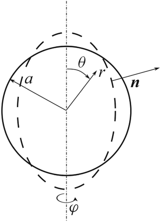
We study the weakly nonlinear shape oscillations of an inviscid liquid drop as sketched in figure 1. The drop is assumed to be axisymmetric with respect to the azimuthal angular coordinate  $\varphi$ of the spherical coordinate system. We treat the liquid as incompressible, and the velocity field is irrotational. The dynamic influence from the ambient medium is neglected. Body forces are not accounted for, since the Froude number is large. The problem is formulated in spherical coordinates to account for its geometry.
Sketch of the geometry of a liquid drop under deformation at mode  $2$.

The equations of change are non-dimensionalised with the undeformed drop radius  $a$, the capillary time scale
 $(\rho a^{3} / \sigma )^{1/2}$ and the capillary pressure
 $\sigma / a$. Here,
 $\rho$ is the liquid density and
 $\sigma$ the surface tension. The drop surface is described by the radial position
 $r_s(\theta ,t) = 1 + \eta (\theta ,t)$, with the non-dimensional deformation
 $\eta$ measured with respect to the unperturbed sphere.
For the problem at hand, the equation of continuity and the two components of the momentum equation in the radial  $(r)$ and polar angular
 $(\theta )$ directions read
 $$\begin{gather} \frac{1}{r^{2}} \frac{\partial}{\partial r} ( r^{2} u_r ) + \frac{1}{r \sin \theta} \frac{\partial}{\partial \theta} ( u_\theta \sin \theta ) = 0, \end{gather}$$
 $$\begin{gather}\frac{\partial u_r}{\partial t} + u_r \frac{\partial u_r}{\partial r} + \frac{u_\theta}{r} \frac{\partial u_r}{\partial \theta} - \frac{u_{\theta}^{2}}{r} ={-} \frac{\partial p}{\partial r}, \end{gather}$$
 $$\begin{gather}\frac{\partial u_\theta}{\partial t} + u_r \frac{\partial u_\theta}{\partial r} + \frac{u_\theta}{r} \frac{\partial u_\theta}{\partial \theta} + \frac{u_r u_\theta}{r} ={-} \frac{1}{r} \frac{\partial p}{\partial \theta}. \end{gather}$$
This set of equations is solved subject to boundary and initial conditions. The kinematic boundary condition states that the material rate of deformation of the drop surface equals the radial velocity component at the place of the deformed surface, i.e.
 \begin{equation} u_r = \frac{\textrm{D} \eta}{\textrm{D}t} = \frac{\partial \eta}{\partial t} + \frac{u_\theta}{r} \frac{\partial \eta}{\partial \theta} \quad \mbox{at } r = 1 + \eta.\end{equation}
The dynamic boundary condition for the inviscid drop states that the stress normal to the drop surface differs across the interface by the contribution of surface tension. This boundary condition reads
 \begin{equation} -p + ( {\boldsymbol \nabla} \boldsymbol{\cdot} {\boldsymbol n} ) = 0 \quad \mbox{at } r = 1 + \eta.\end{equation}
We obtain the divergence of the normal unit vector as
 \begin{align} ( {\boldsymbol \nabla}
\boldsymbol{\cdot} {\boldsymbol n} ) &= \frac{1}{r}
\frac{\displaystyle 2 + 3 \left( \frac{1}{r} \frac{\partial
\eta}{\partial \theta} \right)^{2}}{\displaystyle \left[ 1
+ \left( \frac{1}{r} \frac{\partial \eta}{\partial \theta}
\right)^{2} \right]^{3/2}}\nonumber\\ &\quad - \frac{1}{r^{2} \sin \theta}
\frac{\partial}{\partial \theta} \left[ \frac{\partial
\eta}{\partial \theta} \left( 1+ \left( \frac{1}{r}
\frac{\partial \eta}{\partial \theta} \right)^{2}
\right)^{-{1}/{2}} \sin \theta \right] \quad \mbox{at } r =
1 + \eta. \end{align}
For analysing these equations in a weakly nonlinear form, the two velocity components and the pressure in the flow field, as well as the deformed interface shape, are expanded in power series of the small deformation parameter  $\eta _0$, which plays the role of an initial deformation amplitude. We therefore formulate the expansions of the flow field properties, for example
 $u_r$,
 $p$ and
 $\eta$, as
 $$\begin{gather} u_r = u_{r1} \eta_0 + u_{r2} \eta_0^{2} + u_{r3} \eta_0^{3} + \cdots, \end{gather}$$
 $$\begin{gather}p = p_{1} \eta_0 + p_{2} \eta_0^{2} + p_{3} \eta_0^{3} + \cdots, \end{gather}$$
 $$\begin{gather}\eta = \eta_{1} \eta_0 + \eta_{2} \eta_0^{2} + \eta_{3} \eta_0^{3} + \cdots . \end{gather}$$
For these series expansions to converge, the deformation parameter  $\eta _0$ must be small. One important difference between the linear and the weakly nonlinear analysis is that, in the latter, the boundary conditions are satisfied on the deformed drop surface, not on the unperturbed spherical shape. To achieve this, whilst allowing the functions in the boundary conditions to be evaluated at
 $r = 1$, the values of the functions on the deformed shape are represented by Taylor expansions, such as, for example for
 $u_r$ and
 $p$,
 $$\begin{gather} u_r |_{r=1+\eta} = u_r |_{r=1} + \left. \frac{\partial u_r}{\partial r} \right|_{r=1} \eta + \cdots , \end{gather}$$
 $$\begin{gather}p |_{r=1+\eta} = p |_{r=1} + \left. \frac{\partial p}{\partial r} \right|_{r=1} \eta + \cdots . \end{gather}$$
In integrations with respect to time for determining contributions to the second- and third-order solutions, secular terms appear, which are unphysical. To suppress those terms, the method of strained time is applied (Yuen Reference Yuen1968). The strained time  $\tau$ relates to the physical time
 $t$ as per
 \begin{equation} \tau = \nu t. \end{equation}
The coefficient  $\nu$ is expanded with respect to the amplitude parameter
 $\eta _0$ as per
 \begin{equation} \nu = \nu_{0} + \nu_{1}\eta_{0}+\nu_{2}\eta_{0}^{2} + \cdots. \end{equation}
The new time coordinate contributes to a frequency decrease in the oscillatory motion of the drop, as will be seen later. For the two-lobed mode of motion, the frequency decrease is visible only when taking the approximation to third order. Substituting these approaches into the governing equations (2.1)–(2.3) and into the boundary conditions (2.4) and (2.5), and representing the flow properties and their derivatives as given in (2.7) through (2.11), we obtain sets of first-, second- and third-order equations of motion, with the boundary conditions, by collecting all the terms with the deformation parameter  $\eta _0$ to the first, second and third powers, respectively.
The first initial condition states that the initial deformation of the drop surface is governed by a Legendre polynomial of degree  $m$ with the amplitude
 $\eta _0$. Calculation of the volume of this deformed drop leads to the expression
 \begin{align} r_s(\theta,0) &= 1 + \eta(\theta,0) \nonumber\\ &= \left( 1 + \frac{3 \eta_0^{2}}{2m + 1} + \frac{1}{2}\eta_{0}^{3}\int_{{-}1}^{1}{P_{m}(\cos\theta)}^{3} \, {\textrm{d}} (\cos\theta) \right)^{{-}1/3} + \eta_0 P_m (\cos\theta) \nonumber\\ &= 1 + \eta_0 P_m (\cos\theta) - \eta_0^{2} \frac{1}{2m + 1} - \frac{\eta_{0}^{3}}{6} \int_{{-}1}^{1} {P_{m}(\cos\theta)}^{3} \, {\textrm{d}} (\cos\theta) \mp \cdots , \end{align}
for the initial non-dimensional drop shape. The second initial condition states that the drop surface initially is at rest.
2.1. First-order equations
To obtain the first-order equations with their boundary and initial conditions, the above series expansions are introduced into the respective equations, and all the terms with the parameter  $\eta _0$ to the first power are collected. The first-order continuity and momentum equations read
 $$\begin{gather} \frac{1}{r^{2}} \frac{\partial}{\partial r} ( r^{2} u_{r1} ) + \frac{1}{r \sin \theta} \frac{\partial}{\partial \theta} ( u_{\theta 1} \sin \theta ) = 0 , \end{gather}$$
 $$\begin{gather}\nu_{0}\frac{\partial u_{r1}}{\partial \tau} ={-} \frac{\partial p_1}{\partial r} , \end{gather}$$
 $$\begin{gather}\nu_{0}\frac{\partial u_{\theta 1}}{\partial \tau} ={-} \frac{1}{r} \frac{\partial p_1}{\partial \theta}. \end{gather}$$
For the kinematic and normal-stress boundary conditions of first order at  $r = 1$ we obtain
 $$\begin{gather} u_{r1} = \nu_{0}\frac{\partial \eta_1}{\partial \tau}, \end{gather}$$
 $$\begin{gather}-p_1 - \left( 2 \eta_1 + \frac{\partial \eta_1}{\partial \theta} \cot \theta + \frac{\partial^{2} \eta_1}{\partial \theta^{2}} \right) = 0, \end{gather}$$
respectively. Furthermore, the initial conditions of first order are
 \begin{equation} \eta_1(\theta,0) = P_m (\cos\theta) \quad \mbox{and} \quad \nu_{0}\frac{\partial \eta_1}{\partial \tau} (\theta,0) = 0.\end{equation}
The first initial condition determines the initial shape of the deformed drop, governed by a Legendre polynomial of order  $m$.
2.2. Second-order equations
The second-order equations with their boundary and initial conditions are obtained as all the terms from the expansion with the parameter  $\eta _0$ to the second power. The second-order continuity and momentum equations read
 $$\begin{gather} \frac{1}{r^{2}} \frac{\partial}{\partial r} ( r^{2} u_{r2} ) + \frac{1}{r \sin \theta} \frac{\partial}{\partial \theta} ( u_{\theta 2} \sin \theta ) = 0, \end{gather}$$
 $$\begin{gather}\nu_{0} \frac{\partial u_{r2}}{\partial \tau} + \frac{\partial p_2}{\partial r} = \frac{u_{\theta 1}^{2}}{r} - \nu_{1} \frac{\partial u_{r1}}{\partial \tau} - u_{r1} \frac{\partial u_{r1}}{\partial r} - \frac{u_{\theta 1}}{r}\frac{\partial u_{r1}}{\partial \theta}, \end{gather}$$
 $$\begin{gather}\nu_{0}\frac{\partial u_{\theta 2}}{\partial \tau} + \frac{1}{r} \frac{\partial p_2}{\partial \theta} ={-} \nu_{1}\frac{\partial u_{\theta 1}}{\partial \tau} - u_{r1} \frac{\partial u_{\theta 1}}{\partial r} - \frac{u_{\theta 1}}{r} \frac{\partial u_{\theta 1}}{\partial \theta} - \frac{u_{r1} u_{\theta 1}}{r}. \end{gather}$$
The kinematic and zero normal-stress boundary conditions of second order to be satisfied at  $r = 1$ are
 $$\begin{gather} u_{r2} - \nu_{0}\frac{\partial \eta_2}{\partial \tau} = \nu_{1}\frac{\partial \eta_1}{\partial \tau} + \frac{u_{\theta 1}}{r} \frac{\partial \eta_1}{\partial \theta} - \eta_1 \frac{\partial u_{r1}}{\partial r}, \end{gather}$$
 $$\begin{gather}-p_2 - \left( 2 \eta_2 + \frac{\partial \eta_2}{\partial \theta} \cot \theta + \frac{\partial^{2} \eta_2}{\partial \theta^{2}} \right) = \eta_1 \frac{\partial p_1}{\partial r} - 2 \eta_1^{2} - 2 \eta_1 \frac{\partial \eta_1}{\partial \theta} \cot \theta - 2 \eta_1 \frac{\partial ^{2} \eta_1}{\partial \theta^{2}}. \end{gather}$$
The initial conditions of second order are
 \begin{equation} \eta_2(\theta,0) ={-} \frac{1}{2m + 1} \quad \mbox{and} \quad \nu_{0}\frac{\partial \eta_2}{\partial \tau} (\theta,0) + \nu_{1}\frac{\partial \eta_1}{\partial \tau} (\theta,0) = 0.\end{equation}
The first initial condition ensures volume conservation for the deformed drop to second order. Solving the sets of first- and second-order equations together with their boundary and initial conditions will reveal the nonlinear effect of unequal time spent in the prolate and oblate shapes as a function of the initial deformation amplitude. These solutions reveal the frequency decrease only for initial deformation modes  $m > 2$. To find the frequency decrease for the two-lobed mode
 $m=2$, the theory must be taken to third order, as will be shown below.
2.3. Third-order equations
The third-order continuity and momentum equations read
 \begin{gather} \frac{1}{r^{2}}
\frac{\partial}{\partial r} ( r^{2} u_{r3} ) + \frac{1}{r
\sin \theta} \frac{\partial}{\partial \theta} ( u_{\theta
3} \sin \theta ) = 0,\\\nonumber\end{gather}
 \begin{align} &\nu_{0}\frac{\partial
u_{r 3}}{\partial \tau} + \frac{\partial p_{3}}{\partial r}
={-} \nu_{1}\frac{\partial u_{r 2}}{\partial \tau} -
\nu_{2}\frac{\partial u_{r 1}}{\partial \tau} +
2\frac{u_{\theta 1}u_{\theta 2}}{r} \nonumber\\ & \quad\qquad\qquad\qquad -
u_{r1}\frac{\partial u_{r2}}{\partial r} -
u_{r2}\frac{\partial u_{r1}}{\partial r} - \frac{u_{\theta
1}}{r}\frac{\partial u_{r2}}{\partial \theta} -
\frac{u_{\theta 2}}{r}\frac{\partial u_{r1}}{\partial
\theta}, \\ &\nu_{0}\frac{\partial
u_{\theta 3}}{\partial \tau} + \frac{1}{r}\frac{\partial
p_{3}}{\partial \theta} ={-} \nu_{1}\frac{\partial
u_{\theta 2}}{\partial \tau} - \nu_{2}\frac{\partial
u_{\theta 1}}{\partial \tau} -\frac{u_{r1}u_{\theta 2}}{r}
- \frac{u_{r2}u_{\theta 1}}{r} \nonumber\\ &\qquad\qquad\qquad\qquad\!\! -
u_{r1}\frac{\partial u_{\theta 2}}{\partial r} -
u_{r2}\frac{\partial u_{\theta 1}}{\partial r} -
\frac{u_{\theta 1}}{r}\frac{\partial u_{\theta 2}}{\partial
\theta} - \frac{u_{\theta 2}}{r}\frac{\partial u_{\theta
1}}{\partial \theta}. \end{align}
The third-order kinematic and zero normal-stress boundary conditions, which must be satisfied at  $r=1$, are
 \begin{align} & u_{r 3} -
\nu_{0}\frac{\partial \eta_{3}}{\partial \tau} =
\nu_{1}\frac{\partial \eta_{2}}{\partial \tau} +
\nu_{2}\frac{\partial \eta_{1}}{\partial \tau} +
\frac{u_{\theta 1}}{r} \frac{\partial \eta_2}{\partial
\theta} + \frac{u_{\theta 2}}{r} \frac{\partial
\eta_1}{\partial \theta} + \frac{\partial}{\partial
r}\left(\frac{u_{\theta 1}}{r}\right)\frac{\partial
\eta_{1}}{\partial \theta}\eta_{1} \nonumber\\ &\qquad\qquad\qquad -
\frac{\partial u_{r2}}{\partial r}\eta_1 - \frac{\partial
u_{r1}}{\partial r} \eta_2 - \frac{1}{2}\frac{\partial^{2}
u_{r1}}{\partial
r^{2}}\eta_{1}^{2},\end{align}
 \begin{align} &-p_{3} - \left( 2 \eta_3 + \frac{\partial \eta_3}{\partial \theta} \cot \theta + \frac{\partial^{2} \eta_3}{\partial \theta^{2}} \right) = \frac{\partial p_{1}}{\partial r}\eta_{2} + \frac{\partial p_{2}}{\partial r}\eta_{1} + \frac{1}{2}\frac{\partial^{2}p_{1}}{\partial r^{2}}\eta_{1}^{2} \nonumber\\ &\quad - \eta_{1}^{3} - 2\eta_{1}\left(\eta_{2} + \frac{\partial \eta_{2}}{\partial \theta} \cot \theta + \frac{\partial^{2} \eta_{2}}{\partial \theta^{2}} \right) - 2\eta_{2}\left(\eta_{1} + \frac{\partial \eta_{1}}{\partial \theta} \cot \theta + \frac{\partial^{2} \eta_{1}}{\partial \theta^{2}} \right) \nonumber\\ &\quad - \frac{1}{2}\left(\frac{\partial\eta_{1}}{\partial\theta}\right)^{2}\left(\frac{\partial \eta_{1}}{\partial\theta}\cot\theta + 3\frac{\partial^{2}\eta_{1}}{\partial\theta^{2}}\right) + 3\eta_{1}^{2}\left(\eta_{1} + \frac{\partial\eta_{1}}{\partial\theta}\cot\theta + \frac{\partial^{2}\eta_{1}}{\partial\theta^{2}}\right), \end{align}
respectively. Furthermore, the third-order initial conditions are
 \begin{align} \eta_3(\theta,0) ={-}\frac{1}{3}\begin{pmatrix} m & m & m \\ 0 & 0 & 0 \end{pmatrix}^{2} \quad \mbox{and} \quad \left(\nu_{0}\frac{\partial \eta_3}{\partial \tau}+\nu_{1}\frac{\partial \eta_2}{\partial \tau}+\nu_{2}\frac{\partial \eta_1}{\partial \tau}\right) (\theta,0) = 0,\end{align}
where the first initial condition is described in terms of the 3- $j$ symbols (see the supplementary material available at https://doi.org/10.1017/jfm.2021.568). Solving the sets of equations up to third order together with their boundary and initial conditions will reveal the weakly nonlinear dependency of the angular oscillation frequency on the amplitude of the initial drop deformation. This effect becomes visible due to the strained time introduced for suppressing secular terms in solutions.
3. Solutions of the governing equations
3.1. First-order solutions
The first-order equations describe the linear problem. The well known solutions in Rayleigh (Reference Rayleigh1879) and Lamb (Reference Lamb1881) for the inviscid drop in a vacuum are expected to be recovered. Since we investigate two-dimensional flow fields, the Stokesian stream function is applied for determining the first-order velocity field. We set the coefficient  $\nu _{0}$ in the strained time to unity. The stream function
 $\psi (r,\theta ,\tau )$ is defined by its relations to the two velocity components
 $u_{r1}$ and
 $u_{\theta 1}$ as (Bird, Stewart & Lightfoot Reference Bird, Stewart and Lightfoot1962)
 \begin{equation} u_{r 1} ={-} \frac{1}{r^{2} \sin \theta} \frac{\partial \psi}{\partial \theta} \quad \mbox{and} \quad u_{\theta 1} = \frac{1}{r \sin \theta} \frac{\partial \psi}{\partial r}. \end{equation}
These first-order velocity components satisfy the continuity equation identically.
The first-order drop surface deformation is governed by the Legendre polynomial of the initial deformation. The solution is therefore sought in the form
 \begin{equation} \eta_1 = {\hat \eta}_1 P_m (\cos\theta) \, \textrm{e}^{- \alpha_m \tau}, \end{equation}
with the first-order initial surface amplitude  ${\hat \eta }_1$ and the first-order angular frequency
 $\alpha _m$ for the deformation mode
 $m$.
Taking the curl of the vectorial first-order momentum equation with the components (2.16) and (2.17), the partial differential equation
 \begin{equation} \frac{\partial^{2} \psi}{\partial r^{2}} + \frac{\sin\theta}{r^{2}}\frac{\partial}{\partial\theta} \left( \frac{1}{\sin\theta} \frac{\partial \psi}{\partial \theta} \right) = 0, \end{equation}
for the stream function is obtained. Its solution, which is regular at  $r=0$, reads (Brenn Reference Brenn2017)
 \begin{equation} \psi = C_{1m} r^{m+1} \sin^{2} \theta ~P'_m (\cos\theta) \, \textrm{e}^{-\alpha_m \tau}, \end{equation}
where the prime denotes the derivative of the Legendre polynomial  $P_m$ with respect to its argument. The radial and angular components of the first-order velocity vector follow as
 \begin{equation} u_{r 1} ={-} C_{1m} r^{m-1} m(m+1) P_m (\cos\theta) \, \textrm{e}^{-\alpha_{m} \tau} \end{equation}
and
 \begin{equation} u_{\theta 1} ={-} C_{1m} r^{m-1} (m+1) P_{m}^{1} (\cos\theta) \, \textrm{e}^{-\alpha_{m} \tau}, \end{equation}
respectively. The function  $P_{m}^{1}$ is a Legendre function of degree
 $m$ and order one. The integration constant
 $C_{1m}$ is determined by the first-order kinematic boundary condition as
 \begin{equation} C_{1m} = \frac{\alpha_{m} {\hat \eta}_{1}}{m(m+1)}.\end{equation}
The first-order pressure field is obtained by integration of one component of the momentum equation as
 \begin{equation} p_1 ={-} C_{1m} \alpha_{m} (m+1) r^{m} P_m (\cos\theta) \, \textrm{e}^{-\alpha_{m} \tau}. \end{equation}
The characteristic equation of the drop, which determines the complex angular frequency  $\alpha _m$, follows from the first-order zero normal stress boundary condition (2.19), as obtained in Rayleigh (Reference Rayleigh1879). Its complex conjugate solutions are
 \begin{align} \alpha_{m}^{(p)} = i \sqrt{m(m-1)(m+2)} =: i\, \alpha_{m,0}, \qquad \alpha_{m}^{(n)} ={-}i \sqrt{m(m-1)(m+2)} =: -i\, \alpha_{m,0},\end{align}
where the superscripts  $(p)$ and
 $(n)$ represent the positive and negative solutions, respectively. The existence of pairs of solutions of the characteristic equation requires representation in the first-order solutions. We therefore formulate the first-order deformation of the drop surface as
 \begin{equation} \eta_1 (\theta, \tau) = ( {\hat \eta}_1^{(p)} \, \textrm{e}^{- \alpha_m^{(p)} \tau} + {\hat \eta}_1^{(n)} \, \textrm{e}^{- \alpha_m^{(n)} \tau} ) P_m (\cos\theta). \end{equation}
The first-order initial conditions (2.20a,b) require that initially the drop surface shape is governed by the function  $P_m (\cos\theta )$, and that the surface is at rest. These conditions reveal the deformation amplitudes
 \begin{equation} {\hat \eta}_1^{(p)} ={-} \frac{\alpha_m^{(n)}}{\alpha_m^{(p)} - \alpha_m^{(n)}} = \frac{1}{2} \quad \mbox{ and} \quad {\hat \eta}_1^{(n)} = \frac{\alpha_m^{(p)}}{\alpha_m^{(p)} - \alpha_m^{(n)}} = \frac{1}{2}.\end{equation}
The first-order radial and polar velocity components are represented as
 \begin{equation} u_{r 1}(r, \theta, \tau)={-} (C_{1m}^{(p)}\, \textrm{e}^{-\alpha_{m}^{(p)} \tau} + C_{1m}^{(n)}\, \textrm{e}^{-\alpha_{m}^{(n)} \tau}) r^{m-1} m(m+1) P_m (\cos\theta) \end{equation}
and
 \begin{equation} u_{\theta 1}(r, \theta, \tau) ={-} (C_{1m}^{(p)}\, \textrm{e}^{-\alpha_{m}^{(p)} \tau} + C_{1m}^{(n)}\, \textrm{e}^{-\alpha_{m}^{(n)} \tau}) r^{m-1} (m+1) P_{m}^{1} (\cos\theta), \end{equation}
respectively. The first-order pressure field is
 \begin{equation} p_1 (r, \theta, \tau)={-} (C_{1m}^{(p)} \alpha_{m}^{(p)} \, \textrm{e}^{-\alpha_{m}^{(p)} \tau} + C_{1m}^{(n)} \alpha_{m}^{(n)} \, \textrm{e}^{-\alpha_{m}^{(n)} \tau}) (m+1) r^{m} P_m (\cos\theta) . \end{equation}
With account for the complex conjugate frequencies in (3.9a,b), the first-order drop surface shape, velocity components and pressure field simplify to the forms
 $$\begin{gather} u_{r 1}(r, \theta, \tau) ={-}\, \alpha_{m,0} r^{m-1} P_m\, (\cos\theta) \sin (\alpha_{m,0} \tau), \end{gather}$$
 $$\begin{gather}u_{\theta 1}(r, \theta, \tau) ={-} \frac{\alpha_{m,0}}{m} r^{m-1} P_{m}^{1} (\cos\theta) \sin (\alpha_{m,0} \tau), \end{gather}$$
 $$\begin{gather}p_{1} (r, \theta, \tau) = (m-1)(m+2) r^{m} P_{m} (\cos\theta) \cos (\alpha_{m,0} \tau), \end{gather}$$
 $$\begin{gather}\eta_1 (\theta, \tau) = P_m (\cos\theta) \cos (\alpha_{m,0} \tau). \end{gather}$$
3.2. Second-order solutions
We start developing the second-order solutions from pressure. The general solution for the second-order pressure is sought as a sum
 \begin{equation} p_2 (r,\theta,\tau) = {p}_{21}(r,\theta,\tau) + {p}_{22}(r,\theta,\tau), \end{equation}
of two contributions, where subscript ‘21’ indicates the solution of the system of second-order equations including the products of first-order terms, and subscript ‘22’ the solutions of the homogeneous system. In the second-order approximation, the coefficient  $\nu _{1}$ in the strained time is unknown and needs to be determined.
The solutions with subscripts ‘21’ are first determined. It is convenient to form the divergence of the vectorial second-order momentum equation with the components (2.22) and (2.23) to eliminate the second-order velocity and the terms exhibiting  $\nu _{1}$ with use of the continuity equation (2.21). This yields the differential equation for the second-order pressure
 $p_{21}$,
 \begin{align} &\frac{1}{r^{2}} \frac{\partial}{\partial r} \left( r^{2} \frac{\partial p_{21}}{ \partial r} \right) + \frac{1}{r \sin \theta} \frac{\partial}{\partial \theta} \left( \frac{\sin \theta}{r} \frac{\partial p_{21}}{ \partial \theta} \right) \nonumber\\ &\quad ={-} \frac{1}{r^{2}} \frac{\partial}{\partial r} \left[ r^{2} \left( u_{r1} \frac{\partial u_{r1}}{\partial r} + \frac{u_{\theta 1}}{r} \frac{\partial u_{r1}}{\partial \theta} - \frac{u_{\theta 1}^{2}}{r} \right) \right] \nonumber\\ &\qquad - \frac{1}{r \sin \theta} \frac{\partial}{\partial \theta} \left[ \left( u_{r1} \frac{\partial u_{\theta 1}}{\partial r} + \frac{u_{\theta 1}}{r} \frac{\partial u_{\theta 1}}{\partial \theta} + \frac{u_{r1} u_{\theta 1}}{r} \right) \sin \theta \right], \end{align}
which we rewrite, using the Lamé identity and accounting for the curl-free first-order velocity field, in the form
 \begin{equation} \varDelta [ p_{21} + {\boldsymbol v}_1^{2} / 2 ] = 0 ,\end{equation}
which states that the modified pressure  ${\mathcal {P}}_{21} = p_{21} + {\boldsymbol v}_1^{2}/2$ is potential. The squared first-order velocity vector determines the time dependency of pressure
 $p_{21}$.
The solution of the Laplace equation for the modified pressure  ${\mathcal {P}}_{21}$, formulated in the contribution
 $p_{21}$ to the second-order pressure, accounting for all the time dependencies arising from the square of the first-order velocity vector may be written as
 \begin{align} p_{21}(r,\theta,\tau) & ={-} \sum _{l=0}^{L} (C_{21l}^{(p)}\, \textrm{e}^{{-}2\alpha_{m}^{(p)}\tau} + C_{21l}^{(n)}\, \textrm{e}^{{-}2\alpha_{m}^{(n)}\tau} + C_{21l}^{(pn)}\, \textrm{e}^{-(\alpha_{m}^{(p)} + \alpha_{m}^{(n)}) \tau} ) r^{l}P_{l}(\cos\theta) \nonumber\\ &\quad - \frac{1}{2}(u_{r1}^{2} + u_{\theta 1}^{2}). \end{align}
The coefficients  $C_{21l}^{(pn)}$ relating to time-independent terms in
 $p_{21}$ are set to zero for all
 $l$. This treatment of these coefficients is justified after the calculation of the radial velocity in the next step. All the summations arising in the solutions henceforth extend to an upper summation index symbolised by an uppercase letter. Rewriting the radial momentum equation (2.22) with the modified pressure for the contribution ‘21’, and knowing that the first-order velocity field is irrotational, one obtains
 \begin{equation} \frac{\partial u_{r21}}{\partial \tau} ={-} \frac{\partial {\mathcal{P}}_{21}}{\partial r} - \nu_{1} \frac{\partial u_{r1}}{\partial \tau}. \end{equation}
From this equation, the radial velocity component  $u_{r21}$ is calculated by integration with respect to time, revealing
 \begin{equation} u_{r21}(r,\theta,\tau) ={-} \sum _{l=0}^{L} \left(\frac{C_{21l}^{(p)}}{2 \alpha_{m}^{(p)}}\, \textrm{e}^{{-}2\alpha_{m}^{(p)} \tau} + \frac{C_{21l}^{(n)}}{2 \alpha_{m}^{(n)}} \, \textrm{e}^{{-}2\alpha_{m}^{(n)} \tau}\right) l r^{l-1} P_{l}(\cos\theta) - \nu_{1} u_{r1}. \end{equation}
Non-zero coefficients  $C_{21l}^{(pn)}$ in the pressure
 $p_{21}$ would have produced linearly time-dependent secular terms, which would grow in time. Setting the coefficients
 $C_{21l}^{(pn)}$ for all
 $l$ to zero in (3.22) prevents this. The velocity component
 $u_{\theta 21}$ is then obtained from the continuity equation and reads
 \begin{equation} u_{\theta 21}(r,\theta,\tau ) ={-}\sum _{l=0}^{L}\left(\frac{C_{21l}^{(p)}}{2 \alpha_{m}^{(p)}} \, \textrm{e}^{{-}2\alpha_{m}^{(p)} \tau} + \frac{C_{21l}^{(n)}}{2 \alpha_{m}^{(n)}} \, \textrm{e}^{{-}2\alpha_{m}^{(n)} \tau}\right) r^{l-1}P_{l}^{1}(\cos\theta) - \nu_{1} u_{\theta 1}. \end{equation}
Following the work by Tsamopoulos & Brown (Reference Tsamopoulos and Brown1983, Reference Tsamopoulos and Brown1984), the surface deformation  $\eta _{21}$ is written in a general form as
 \begin{equation} \eta_{21}(\theta,\tau ) = \sum_{l=0}^{L} \delta_{2l}(\tau) P_{l}(\cos\theta) , \end{equation}
where the time dependency is governed by the unknown functions  $\delta _{2l} (\tau )$, and the deformed shape by all possible Legendre polynomials. The reason for the latter is that, in the zero normal-stress boundary condition, pressure and surface deformation are coupled. The functions
 $\delta _{2l}(\tau )$ are determined for every
 $l$ using the boundary conditions (2.24) and (2.25). For doing this,
 $u_{r21}$ and
 $\eta _{21}$ from (3.24) and (3.26), respectively, are substituted into the kinematic boundary condition (2.24). Its derivative with respect to the strained time
 $\tau$ is taken. We substitute the pressure
 $p_{21}$ and
 $\eta _{21}$, from (3.22) and (3.26), respectively, into the zero normal-stress boundary condition (2.25). Since we deal with the boundary conditions,
 $r=1$ in both equations. We proceed by multiplying the two equations with a Legendre polynomial
 $P_{j}$ and integrating the results between the south and north poles of the drop. Multiplying the equation resulting from the zero-normal stress boundary condition by the natural number
 $j$ and subtracting the two resulting equations eliminates the coefficients
 $C_{21j}$ for all time dependencies, yielding the ordinary differential equation
 \begin{align} & {\ddot \delta}_{2j}(\tau) + j(\,j - 1)(\,j + 2)\delta_{2j}(\tau) =\left[ - \nu_{1} ({\alpha_{m}^{(p)}}^{2} \, \textrm{e}^{-\alpha_{m}^{(p)} \tau} + {\alpha_{m}^{(n)}}^{2} \, \textrm{e}^{-\alpha_{m}^{(n)} \tau}) \int_{{-}1}^{1} P_{m} P_{j}\, {\textrm{d}\kern0.7pt x} \right. \nonumber\\ &\quad - \left. \int_{{-}1}^{1} \frac{\partial }{\partial \tau}\left( \frac{u_{\theta 1}}{r} \frac{\partial \eta_1}{\partial \theta} - \eta_1 \frac{\partial u_{r1}}{\partial r}\right) \right|_{r=1} P_{j}\, {\textrm{d}\kern0.7pt x} \nonumber\\ &\quad + \int_{{-}1}^{1} \left.\left.\left(Rz_{21} - \frac{1}{2}(u_{r1}^{2} + u_{\theta 1}^{2})\right) \right|_{r=1} j P_{j}\, {\textrm{d}\kern0.7pt x} \right] \frac{2j + 1}{2} , \end{align}
for  $\delta _{2j}(\tau )$ (Tsamopoulos & Brown Reference Tsamopoulos and Brown1983, Reference Tsamopoulos and Brown1984), where
 $Rz_{21}$ is the right-hand side of the zero normal-stress boundary condition (2.25). For the differential equation (3.27), we are interested in the particular solutions only, because the homogeneous solutions will be accounted for by the second-order contribution ‘22’. The particular solutions need to be found for every
 $j$ between zero and
 $L$. Introducing back all particular solutions
 $\delta _{2j}(\tau )$ of (3.27) into (3.26), we can write the final form as
 \begin{align} \eta_{21}(\theta, \tau ) &= \sum _{j=0}^{L} (H_{21j}^{(p)}\, \textrm{e}^{{-}2\alpha_{m}^{(p)} \tau} + H_{21j}^{(n)}\, \textrm{e}^{{-}2\alpha_{m}^{(n)} \tau} + H_{21j}^{(pn)}\, \textrm{e}^{-(\alpha_{m}^{(p)} + \alpha_{m}^{(n)}) \tau}) P_{j}(\cos\theta) \nonumber\\ &\quad + \frac{\nu_{1}}{4} [ ( 1 + 2 \alpha_{m}^{(p)} \tau ) \, \textrm{e}^{-\alpha_{m}^{(p)} \tau} + (1+2\alpha_{m}^{(n)}\tau )\, \textrm{e}^{-\alpha_{m}^{(n)} \tau}] P_{m}, \end{align}
where the coefficients  $H_{21j}^{(p)}$,
 $H_{21j}^{(n)}$ and
 $H_{21j}^{(pn)}$ are known. The second part of the solution (3.28), with
 $\nu _1$ in front, exhibits secular terms growing in time. Due to this unphysical behaviour, these terms must be suppressed by setting
 $\nu _{1} = 0$. With the surface deformation
 $\eta _{21}$ known, the coefficients
 $C_{21l}$ in
 $u_{r21}$,
 $u_{\theta 21}$ and
 $p_{21}$ are readily determined, for every time dependency and for all
 $l$ between zero and
 $L$, using one of the boundary conditions (2.24) or (2.25). The details of the calculation of
 $C_{21l}$ are presented in the supplementary material. Now, we can write the contributions ‘
 $21$’ to the second-order solutions in the form
 $$\begin{gather} u_{r21}(r,\theta,\tau) = \sum _{l=0}^{L} \frac{C_{21l}}{\alpha_{m,0}} \sin(2 \alpha_{m,0} \tau ) l r^{l-1} P_{l}(\cos\theta), \end{gather}$$
 $$\begin{gather}u_{\theta 21}(r,\theta,\tau) = \sum _{l=0}^{L} \frac{C_{21l}}{\alpha_{m,0}} \sin(2 \alpha_{m,0} \tau ) r^{l-1}P_{l}^{1}(\cos\theta), \end{gather}$$
 $$\begin{gather}p_{21}(r,\theta,\tau) ={-} 2 \sum _{l=0}^{L} C_{21l} \cos(2 \alpha_{m,0} \tau ) r^{l}P_{l}(\cos\theta) - \frac{1}{2}(u_{r1}^{2} + u_{\theta 1}^{2}), \end{gather}$$
 $$\begin{gather}\eta_{21}(\theta,\tau) = \sum _{l=0}^{L} (2 H_{21l} \cos(2 \alpha_{m,0} \tau ) + H_{21l}^{(pn)}) P_{l}(\cos\theta). \end{gather}$$
The second contributions to the second-order solutions, with subscript ‘22’, are determined from the homogeneous forms of (2.21)–(2.23). This set of equations has the same structure as at first order, where the complex angular frequency  $\alpha _{m}$ is replaced by
 $\alpha _{2k}$ (with the number ‘2’ in the subscript indicating the second-order solution, and
 $k$ a deformation mode number) and the deformation amplitude of the drop surface
 $\hat {\eta }_{1}$ by
 $\hat {\eta }_{22k}$. Both replaced variables appear under a sum with the summation index
 $k$, implying that all possible deformation modes
 $k$ affect the results.
The contributions ‘22’ to the second-order velocity, pressure and deformation are obtained as linear combinations of eigensolutions of the underlying differential equations with the summation index  $k$. Their forms are similar to the first-order solutions and read
 \begin{align} u_{r22}(r,\theta,\tau ) & ={-}\sum _{k=0}^{K}(C_{22k}^{(p)}\, \textrm{e}^{-\alpha_{2k}^{(p)}\tau} + C_{22k}^{(n)}\, \textrm{e}^{-\alpha_{2k}^{(n)}\tau}) \nonumber\\ &\quad \times k(k+1)r^{k-1}P_{k}(\cos\theta) ,\\ u_{\theta 22}(r,\theta, \tau) & ={-}\sum _{k=0}^{K}(C_{22k}^{(p)}\, \textrm{e}^{-\alpha_{2k}^{(p)}\tau} + C_{22k}^{(n)}\, \textrm{e}^{-\alpha_{2k}^{(n)}\tau}) \nonumber\\ &\quad \times (k+1) r^{k-1}P_{k}^{1}(\cos\theta) ,\\ p_{22}(r,\theta,\tau) &={-}\sum _{k=0}^{K}(\alpha_{2k}^{(p)}C_{22k}^{(p)}\, \textrm{e}^{-\alpha_{2k}^{(p)}\tau} + \alpha_{2k}^{(n)} C_{22k}^{(n)}\, \textrm{e}^{-\alpha_{2k}^{(n)}\tau}) \nonumber\\ &\quad \times (k+1)r^{k}P_{k}(\cos\theta), \end{align}
 \begin{align} \eta_{22}(\theta,\tau) &= \sum _{k=0}^{K}(\hat{\eta}_{22k}^{(p)}\, \textrm{e}^{-\alpha_{2k}^{(p)}\tau} + \hat{\eta}_{22k}^{(n)} \, \textrm{e}^{-\alpha_{2k}^{(n)}\tau}) P_{k}(\cos\theta). \end{align}
The two new complex conjugate angular frequencies  $\alpha _{2k}$, obtained as solutions of the homogeneous zero normal-stress boundary condition, for all summation indices
 $k$ take the forms obtained in Rayleigh (Reference Rayleigh1879):
 \begin{align} \alpha_{2k}^{(p)} = i \sqrt{k(k-1)(k+2)} =: i\, \alpha_{2k,0}, \qquad \alpha_{2k}^{(n)} ={-}i \sqrt{k(k-1)(k+2)} =: -i\, \alpha_{2k,0}.\end{align}
The calculations of the coefficients  $C_{22k}$ and of the amplitudes
 $\hat {\eta }_{22k}$ are detailed in the supplementary material.
The contributions ‘22’ to the second-order solutions are obtained in the simplified forms
 $$\begin{gather} u_{r22}(r,\theta,\tau ) ={-} 2 \sum _{k=0}^{K} {\hat \eta}_{22k} \alpha_{2k,0} r^{k-1}P_{k} (\cos\theta) \sin(\alpha_{2k,0} \tau ) , \end{gather}$$
 $$\begin{gather}u_{\theta 22}(r,\theta, \tau) ={-} 2 \sum _{k=1}^{K} \frac{{\hat \eta}_{22k} \alpha_{2k,0}}{k} r^{k-1}P_{k}^{1}(\cos\theta) \sin(\alpha_{2k,0} \tau ) , \end{gather}$$
 $$\begin{gather}p_{22}(r,\theta,\tau) = 2 \sum _{k=0}^{K}{\hat \eta}_{22k} (k - 1)(k + 2) r^{k}P_{k}(\cos\theta) \cos(\alpha_{2k,0} \tau), \end{gather}$$
 $$\begin{gather}\eta_{22}(\theta,\tau) = 2 \sum _{k=0}^{K}{\hat \eta}_{22k} P_{k}(\cos\theta) \cos(\alpha_{2k,0} \tau ). \end{gather}$$
3.3. Third-order solutions
We start developing the third-order solutions also from pressure. The general solution for the third-order pressure is sought as a sum
 \begin{equation} p_{3}(r,\theta,\tau) = p_{31}(r,\theta,\tau) + p_{32}(r,\theta,\tau), \end{equation}
of two contributions, where subscript ‘31’ indicates the solution of the third-order equations system including the products of first- and second-order terms, while the subscript ‘32’ denotes the solutions of the homogeneous system of the governing equations with its boundary and initial conditions. The coefficient  $\nu _{2}$ in the strained time coordinate is unknown and needs to be determined.
The solutions with the subscript ‘31’ are first determined. Taking the divergence of the vectorial third-order momentum equation with the components (2.28) and (2.29), and using the continuity equation (2.27), the third-order velocities are eliminated. The result is the following partial differential equation for the third-order pressure  $p_{31}$:
 \begin{align} & \frac{1}{r^{2}}
\frac{\partial}{\partial r} \left( r^{2} \frac{\partial
p_{31}}{ \partial r} \right) + \frac{1}{r \sin \theta}
\frac{\partial}{\partial \theta} \left( \frac{\sin
\theta}{r} \frac{\partial p_{31}}{ \partial \theta} \right)
\nonumber\\ & \quad ={-} \frac{1}{r^{2}}
\frac{\partial}{\partial r} \left[ r^{2} \left( u_{r1}
\frac{\partial u_{r2}}{\partial r} + u_{r2} \frac{\partial
u_{r1}}{\partial r} + \frac{u_{\theta 1}}{r} \frac{\partial
u_{r2}}{\partial \theta} +\frac{u_{\theta 2}}{r}
\frac{\partial u_{r1}}{\partial \theta} - 2\frac{u_{\theta
1} u_{\theta 2}}{r} \right) \right] \nonumber\\ &\qquad -
\frac{1}{r \sin \theta} \frac{\partial}{\partial \theta}
\left[ \left( u_{r1} \frac{\partial u_{\theta 2}}{\partial
r} + u_{r2} \frac{\partial u_{\theta 1}}{\partial r} +
\frac{u_{\theta 2}}{r} \frac{\partial u_{\theta
1}}{\partial \theta} + \frac{u_{\theta 1}}{r}
\frac{\partial u_{\theta 2}}{\partial \theta} +
\frac{u_{r2} u_{\theta 1}}{r} + \frac{u_{r1} u_{\theta
2}}{r} \right) \sin \theta \right],
\end{align}
which we write in a compact form as
 \begin{equation} \varDelta p_{31} ={-} \textrm{div} [(\boldsymbol{u}_{1}\boldsymbol{\cdot} \boldsymbol{\nabla})\boldsymbol{u}_{2} + (\boldsymbol{u}_{2}\boldsymbol{\cdot} \boldsymbol{\nabla})\boldsymbol{u}_{1}]. \end{equation}
The equation is rewritten using the dot product rule to yield
 \begin{equation} \varDelta {\mathcal{P}}_{31} = \textrm{div} [\boldsymbol{u}_{1}\times(\boldsymbol{\nabla}\times\boldsymbol{u}_{2}) + \boldsymbol{u}_{2}\times(\boldsymbol{\nabla}\times\boldsymbol{u}_{1})], \end{equation}
where the modified pressure is defined as  ${\mathcal {P}}_{31} = p_{31} + \boldsymbol {u}_{1}\boldsymbol {\cdot } \boldsymbol {u}_{2}$. Evidently the right-hand side is zero, since the velocity fields involved are irrotational. We determine the time dependencies of the third-order pressure
 $p_{31}$ following the same procedure as for the second-order modified pressure. Accounting for all the time dependencies arising from the inner product of the first- and second-order velocity fields we write
 \begin{align} p_{31}(r,\theta,\tau) &={-}\sum_{h=0}^{H} r^{h}P_{h}(x) \left( C_{31h}^{(p)} \, \textrm{e}^{{-}3\alpha_{m}^{(p)}\tau} + C_{31h}^{(n)} \, \textrm{e}^{{-}3\alpha_{m}^{(n)}\tau} \vphantom{\sum_{k=0}^{K}} \right.\nonumber\\ &\quad + C_{31h}^{(ppn)} \, \textrm{e}^{-(2\alpha_{m}^{(p)} + \alpha_{m}^{(n)})\tau} + C_{31h}^{(pnn)} \, \textrm{e}^{-(\alpha_{m}^{(p)} + 2\alpha_{m}^{(n)})\tau} \nonumber\\ &\quad + \sum_{k=0}^{K} C_{31hk}^{(pp)}\, \textrm{e}^{-(\alpha_{m}^{(p)} + \alpha_{2k}^{(p)})\tau} + \sum_{k=0}^{K} C_{31hk}^{(nn)}\, \textrm{e}^{-(\alpha_{m}^{(n)} + \alpha_{2k}^{(n)})\tau} \nonumber\\ &\quad + \left.\sum_{k=0}^{K} C_{31hk}^{(pn)}\, \textrm{e}^{-(\alpha_{m}^{(p)} + \alpha_{2k}^{(n)})\tau} + \sum_{k=0}^{K} C_{31hk}^{(np)}\, \textrm{e}^{-(\alpha_{m}^{(n)} + \alpha_{2k}^{(p)})\tau} \right) - \boldsymbol{u}_{1}\boldsymbol{\cdot} \boldsymbol{u}_{2} . \end{align}
The coefficients  $C_{31hm}^{(pn)}$ and
 $C_{31hm}^{(np)}$ relating to time-independent terms in
 $p_{31}$ are set to zero for all
 $h$, following the same reasoning as in the second-order approximation. The contributions ‘31’ to the velocity field are determined by the same procedure as for second order. Rewriting the radial momentum equation (2.28), using that the first- and second-order velocity fields are irrotational, and with the definition of the third-order modified pressure
 ${\mathcal {P}}_{31}$, one obtains
 \begin{equation} \frac{\partial u_{r31}}{\partial \tau} ={-}\frac{\partial{\mathcal{P}}_{31}}{\partial r} - \nu_{2} \frac{\partial u_{r1}}{\partial \tau}. \end{equation}
Integration of this momentum equation with respect to time, with the modified pressure  ${\mathcal {P}}_{31}$ known, yields the radial velocity component
 $u_{31}$ for every time dependency
 \begin{align} u_{r31}(r,\theta,\tau) &={-} \sum _{h=0}^{H} \left( \frac{C_{31h}^{(p)}}{3\alpha_{m}^{(p)}} \, \textrm{e}^{{-}3\alpha_{m}^{(p)}\tau} + \frac{C_{31h}^{(n)}}{3\alpha_{m}^{(n)}} \, \textrm{e}^{{-}3\alpha_{m}^{(n)}\tau} + \frac{C_{31h}^{(ppn)}}{2\alpha_{m}^{(p)} + \alpha_{m}^{(n)}} \, \textrm{e}^{-(2\alpha_{m}^{(p)}+\alpha_{m}^{(n)})\tau} \right. \nonumber\\ &\quad + \frac{C_{31h}^{(pnn)}}{\alpha_{m}^{(p)} + 2\alpha_{m}^{(n)}} \, \textrm{e}^{-(\alpha_{m}^{(p)} + 2\alpha_{m}^{(n)})\tau} + \sum_{k=0}^{K} \frac{C_{31hk}^{(pp)}}{\alpha_{m}^{(p)} + \alpha_{2k}^{(p)}} \, \textrm{e}^{-(\alpha_{m}^{(p)} + \alpha_{2k}^{(p)})\tau} \nonumber\\ &\quad + \sum_{k=0}^{K} \frac{C_{31hk}^{(nn)}}{\alpha_{m}^{(n)} + \alpha_{2k}^{(n)}} \, \textrm{e}^{-(\alpha_{m}^{(n)} + \alpha_{2k}^{(n)})\tau} + \sum_{k=0\backslash m}^{K} \frac{C_{31hk}^{(pn)}}{\alpha_{m}^{(p)} + \alpha_{2k}^{(n)}} \, \textrm{e}^{-(\alpha_{m}^{(p)} + \alpha_{2k}^{(n)})\tau} \nonumber\\ &\quad + \left.\sum_{k=0\backslash m}^{K} \frac{C_{31hk}^{(np)}}{\alpha_{m}^{(n)} + \alpha_{2k}^{(p)}} \, \textrm{e}^{-(\alpha_{m}^{(n)} + \alpha_{2k}^{(p)})\tau}\right)h r^{h-1} P_{h}(\cos\theta) - \nu_{2} u_{r1}. \end{align}
Non-zero coefficients  $C_{31hm}^{(pn)}$ and
 $C_{31hm}^{(np)}$ in the pressure
 $p_{31}$ would have produced linearly time-dependent secular terms, which would grow in time, just as seen at second order. These secular terms are suppressed by this treatment. The polar velocity component is then determined using the continuity equation (2.27) and reads
 \begin{align} u_{\theta 31}(r,\theta,\tau) &={-} \sum _{h=0}^{H} \left( \frac{C_{31h}^{(p)}}{3\alpha_{m}^{(p)}} \, \textrm{e}^{{-}3\alpha_{m}^{(p)}\tau} + \frac{C_{31h}^{(n)}}{3\alpha_{m}^{(n)}} \, \textrm{e}^{{-}3\alpha_{m}^{(n)}\tau} + \frac{C_{31h}^{(ppn)}}{2\alpha_{m}^{(p)} + \alpha_{m}^{(n)}} \, \textrm{e}^{-(2\alpha_{m}^{(p)}+\alpha_{m}^{(n)})\tau} \right. \nonumber\\ &\quad + \frac{C_{31h}^{(pnn)}}{\alpha_{m}^{(p)} + 2\alpha_{m}^{(n)}} \, \textrm{e}^{-(\alpha_{m}^{(p)} + 2\alpha_{m}^{(n)})\tau} + \sum_{k=0}^{K} \frac{C_{31hk}^{(pp)}}{\alpha_{m}^{(p)} + \alpha_{2k}^{(p)}} \, \textrm{e}^{-(\alpha_{m}^{(p)} + \alpha_{2k}^{(p)})\tau} \nonumber\\ &\quad + \sum_{k=0}^{K} \frac{C_{31hk}^{(nn)}}{\alpha_{m}^{(n)} + \alpha_{2k}^{(n)}} \, \textrm{e}^{-(\alpha_{m}^{(n)} + \alpha_{2k}^{(n)})\tau} + \sum_{k=0\backslash m}^{K} \frac{C_{31hk}^{(pn)}}{\alpha_{m}^{(p)} + \alpha_{2k}^{(n)}} \, \textrm{e}^{-(\alpha_{m}^{(p)} + \alpha_{2k}^{(n)})\tau} \nonumber\\ &\quad + \left.\sum_{k=0\backslash m}^{K} \frac{C_{31hk}^{(np)}}{\alpha_{m}^{(n)} + \alpha_{2k}^{(p)}} \, \textrm{e}^{-(\alpha_{m}^{(n)} + \alpha_{2k}^{(p)})\tau}\right) r^{h-1} P_{h}^{1}(\cos\theta) - \nu_{2} u_{\theta 1}. \end{align}
For formulating the surface deformation  $\eta _{31}$, we proceed as in the second-order approximation. Following the work by Tsamopoulos & Brown (Reference Tsamopoulos and Brown1983, Reference Tsamopoulos and Brown1984), the surface deformation is written in a general form as
 \begin{equation} \eta_{31}(\theta,\tau ) = \sum_{h=0}^{H} \delta_{3h}(\tau) P_{h}(\cos\theta), \end{equation}
where the time dependency is governed by the unknown functions  $\delta _{3h} (\tau )$, and the deformed shape by all possible Legendre polynomials. We determine the functions
 $\delta _{3h} (\tau )$ by deriving the governing ordinary differential equation, following the same procedure as in the second-order approximation. The procedure eliminates the coefficients
 $C_{31j}$ and
 $C_{31jk}$ for all time dependencies from the kinematic and zero normal-stress boundary conditions at third order, (2.30) and (2.31), yielding the ordinary differential equation (Tsamopoulos & Brown Reference Tsamopoulos and Brown1983, Reference Tsamopoulos and Brown1984)
 \begin{align} & {\ddot \delta}_{3j}(\tau) + j(\,j - 1)(\,j + 2)\delta_{3j}(\tau) = \frac{2j + 1}{2} \left[\left. - \int_{{-}1}^{1} \frac{\partial Rk_{31}}{\partial \tau}\right|_{r=1} P_{j}\, {\textrm{d}\kern0.7pt x} \right.\nonumber\\ &\quad - \left.\left.\frac{\nu_{2}}{2} ({\alpha_{m}^{(p)}}^{2} \, \textrm{e}^{-\alpha_{m}^{(p)} \tau} + {\alpha_{m}^{(n)}}^{2} \, \textrm{e}^{-\alpha_{m}^{(n)} \tau}) \int_{{-}1}^{1} P_{m} P_{j}\, {\textrm{d}\kern0.7pt x} + \int_{{-}1}^{1} (Rz_{31} - \boldsymbol{u}_1 \boldsymbol{\cdot} \boldsymbol{u}_2)\right|_{r=1} j P_{j}\, {\textrm{d}\kern0.7pt x}\right], \end{align}
for  $\delta _{3j} (\tau )$, where
 $Rk_{31}$ and
 $Rz_{31}$ are the right-hand sides of the two boundary conditions (2.30) and (2.31), respectively. We keep this compact formulation of the equation, since the right-hand sides of the boundary conditions consist of many terms. The calculations and symbolic derivations were performed with the software Mathematica. We are only interested in the particular solutions of (3.51). The general solution of the homogeneous equation will be accounted for by the contribution ‘32’, which solves the homogeneous system of equations. The solutions need to be found for every
 $j$ between zero and
 $H$. Introducing back all the particular solutions
 $\delta _{3j}(\tau )$ of the differential equation (3.51) into (3.50), we can write the final form as
 \begin{align} \eta_{31}(\theta,\tau) &= \sum _{j=0}^{H} \left( H_{31j}^{(p)}\, \textrm{e}^{{-}3\alpha_{m}^{(p)}\tau} + H_{31j}^{(n)}\, \textrm{e}^{{-}3\alpha_{m}^{(n)}\tau} \vphantom{\sum_{k=0}^{K}}\right. \nonumber\\ &\quad + H_{31j}^{(ppn)}\, \textrm{e}^{-(2\alpha_{m}^{(p)} + \alpha_{m}^{(n)})\tau} + H_{31j}^{(pnn)}\, \textrm{e}^{-(\alpha_{m}^{(p)} + 2\alpha_{m}^{(n)})\tau} \nonumber\\ &\quad + \sum_{k=0}^{K} H_{31jk}^{(pp)}\, \textrm{e}^{-(\alpha_{m}^{(p)} + \alpha_{2k}^{(p)})\tau} + \sum_{k=0}^{K} H_{31jk}^{(nn)}\, \textrm{e}^{-(\alpha_{m}^{(n)} + \alpha_{2k}^{(n)})\tau} \nonumber\\ &\quad + \left.\sum_{k=0}^{K} H_{31jk}^{(pn)}\, \textrm{e}^{-(\alpha_{m}^{(p)} + \alpha_{2k}^{(n)})\tau} + \sum_{k=0}^{K} H_{31jk}^{(np)}\, \textrm{e}^{-(\alpha_{m}^{(n)} + \alpha_{2k}^{(p)})\tau} \right) P_{j}(\cos\theta), \end{align}
where the coefficients  $H_{31j}$ and
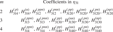
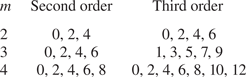
 $H_{31jk}$ for all time dependencies are known. Among them, the coefficients shown in table 1 are set to zero, since the corresponding solutions exhibit secular terms. These solutions must therefore be suppressed as unphysical, and their structure would not correspond to those represented by the above equation. The phenomenon arises because the initial deformation of the mode
 $m$ excites higher-order modes
 $i$, which can be interpreted as a resonance. The secular terms appear in the three cases where
 \begin{equation} \left. \begin{array}{c@{}}
i(i-1)(i+2)/\alpha_{m}^{2} \\ i(i-1)(i+2)/4\alpha_{m}^{2}
\\ i(i-1)(i+2)/9\alpha_{m}^{2} \end{array}
\right\} ={-}1. \end{equation}
Equation (3.51) then assumes the general form
 \begin{equation} \ddot{\delta}_{3i}^{*}(\tau) - c^{2} \delta_{3i}^{*} (\tau) = A \, \textrm{e}^{{-}c \tau}, \end{equation}
with the particular solution
 \begin{equation} \delta_{3i}^{*} (\tau) ={-}\frac{A}{4c^{2}} (1+2 c \tau) \, \textrm{e}^{{-}c\tau}, \end{equation}
where the notation with the asterisk is introduced to indicate the exceptional cases of (3.51) and its solutions. The solutions exhibit in front of the exponential function a linear secular term which grows in time. Secular solutions relating to the first part of the statement (3.53), for which  $i=m$, are due to functions of time on the right-hand sides of (3.51) leading to resonance with the frequency
 $\alpha _m^{(p)}$ or
 $\alpha _m^{(n)}$ appearing in the exponentials. They contain the coefficient
 $\nu _2$ in a linear combination with other, known, quantities represented by the factor
 $A$ in (3.55). For suppressing all these secular solutions, the values of the coefficient
 $\nu _{2}$ are determined for each mode
 $m$ of initial drop deformation such that the solutions vanish. This results in a straining of time, which may be seen equivalent to a change of the oscillation frequency against the first-order motion. The corresponding coefficients are all those listed in table 1 for the various modes
 $m$, except
 $H_{314}^{(p)}$ and
 $H_{314}^{(n)}$.
The coefficients  $H_{31j}$ and
 $H_{31jk}$ in the surface deformation
 $\eta _{31}$ for
 $m = 2,3$ and
 $4$ set to zero since they relate to secular solutions.

The second part of the statement (3.53) appears only for  $m=5$ when
 $i=8$, and for
 $m=10$ when
 $i=16$, corresponding to solutions with the coefficients
 $H_{3185}^{(pp)}$,
 $H_{3185}^{(nn)}$ and
 $H_{311610}^{(pp)}$,
 $H_{311610}^{(nn)}$, respectively. These cases are not treated here, since our analysis is restricted to modes less than
 $m=5$. The third part of the statement appears only for
 $m=2$ when
 $i=4$, with the corresponding two coefficients
 $H_{314}^{(p)}$ and
 $H_{314}^{(n)}$. The secular solutions
 $\delta _{34}^{*}(\tau )$ are due to functions of time on the right-hand sides of (3.51) leading to resonance with the frequency
 $3\alpha _m^{(p)}$ or
 $3\alpha _m^{(n)}$ appearing in the exponentials. In these secular solutions
 $\delta _{34}^{*}(\tau )$, the coefficient
 $\nu _2$ does not occur, so that it cannot be used for suppressing them. Therefore, the coefficients
 $H_{314}^{(p)}$ and
 $H_{314}^{(n)}$ corresponding to this case are set to zero to suppress this secular solution.
With the surface deformation  $\eta _{31}$ known, the coefficients
 $C_{31j}$ and
 $C_{31jk}$ for all time dependencies are calculated using one of the boundary conditions (2.30) or (2.31). The procedure of this coefficient calculation is identical to the second-order approximation. We omit the details of this derivation because it involves large expressions. The final representations of the pressure (3.46), radial velocity (3.48) and polar velocity (3.49) ‘31’ are given in simplified forms as
 \begin{align} p_{31}(r,\theta,\tau)
&={-} 2 \sum_{h=0}^{H} r^{h}P_{h}(x) \left[ C_{31h}^{(1)}
\cos(3 \alpha_{m,0} \tau) + C_{31h}^{(2)}\cos(\alpha_{m,0}
\tau) \vphantom{\sum_{k=0}^{K}}\right. \nonumber\\ &\quad +
\sum_{k=0}^{K} C_{31hk}^{(3)} \cos((\alpha_{2k,0} +
\alpha_{m,0})\tau) \nonumber\\ &\quad + \left.\sum_{k=0
\backslash m}^{K} C_{31hk}^{(4)} \cos((\alpha_{2k,0} -
\alpha_{m,0}) \tau )\right] -
\boldsymbol{u}_{1}\boldsymbol{\cdot} \boldsymbol{u}_{2} ,\end{align}
 \begin{align}
u_{r31}(r,\theta,\tau) &= 2 \sum _{h=0}^{H} h r^{h-1}
P_{h}(\cos\theta) \left[\frac{C_{31h}^{(1)}}{3
\alpha_{m,0}}\sin(3\alpha_{m,0} \tau) +
\frac{C_{31h}^{(2)}}{\alpha_{m,0}}\sin
(\alpha_{m,0}\tau)\right. \nonumber\\ &\quad +
\sum_{k=0}^{K} \frac{C_{31hk}^{(3)}}{\alpha_{2k,0} +
\alpha_{m,0}}\sin((\alpha_{2k,0} + \alpha_{m,0})\tau)
\nonumber\\ &\quad + \left. \sum_{k=0\backslash m}^{K}
\frac{C_{31hk}^{(4)}}{\alpha_{2k,0} - \alpha_{m,0}}
\sin((\alpha_{2k,0} - \alpha_{m,0})\tau) \right] -
\nu_{2}u_{r1}, \end{align}
 \begin{align}
u_{\theta 31}(r,\theta,\tau) & = 2 \sum
_{h=0}^{H} r^{h-1} P_{h}^{1}(\cos\theta)
\left[\frac{C_{31h}^{(1)}}{3
\alpha_{m,0}}\sin(3\alpha_{m,0} \tau) +
\frac{C_{31h}^{(2)}}{\alpha_{m,0}}\sin
(\alpha_{m,0}\tau)\right. \nonumber\\ &\quad +
\sum_{k=0}^{K} \frac{C_{31hk}^{(3)}}{\alpha_{2k,0} +
\alpha_{m,0}}\sin((\alpha_{2k,0} + \alpha_{m,0})\tau)\nonumber\\ &\quad +
\left.\sum_{k=0\backslash m}^{K}
\frac{C_{31hk}^{(4)}}{\alpha_{2k,0} - \alpha_{m,0}}
\sin((\alpha_{2k,0} - \alpha_{m,0})\tau) \right] -
\nu_{2}u_{\theta 1}. \end{align}
The related drop surface deformation reads
 \begin{align} \eta_{31}(\theta,\tau) & = 2 \sum _{h=0}^{H} P_{h}(\cos\theta) \left[ H_{31h}^{(1)}\cos(3\alpha_{m,0} \tau ) + H_{31h}^{(2)}\cos(\alpha_{m,0}\tau) \vphantom{\sum_{k=0}^{K}} \right.\nonumber\\ &\quad + \left.\sum_{k=0}^{K} H_{31hk}^{(3)}\cos((\alpha_{2k,0} + \alpha_{m,0})\tau) + \sum_{k=0}^{K} H_{31hk}^{(4)}\cos((\alpha_{2k,0} - \alpha_{m,0})\tau) \right], \end{align}
where the definitions of the coefficients for the different time dependencies are given in the supplementary material.
Having determined the contributions ‘31’ to the third-order solutions, we move to the contributions ‘32.’ The homogeneous system of the third-order governing equations together with their boundary conditions determine these contributions. The homogeneous system consists of the third-order governing equations (2.27)–(2.29). Its solutions must satisfy the third-order homogeneous boundary conditions (2.30) and (2.31). The solutions are linear combinations of eigensolutions with index  $h$ which are similar to the first order, and the contributions ‘
 $22$’ to the second-order solutions. The velocity components, the pressure field and the deformation of the drop surface read
 \begin{align} u_{r32}(r,\theta,\tau) & ={-}\sum _{h=0}^{H}(C_{32k}^{(p)}\, \textrm{e}^{-\alpha_{3h}^{(p)}\tau} + C_{32h}^{(n)}\, \textrm{e}^{-\alpha_{3h}^{(n)}\tau}) \nonumber\\ &\quad \times h(h+1)r^{h-1}P_{h}(\cos\theta), \end{align}
 \begin{align} u_{\theta 32}(r,\theta,\tau) &={-}\sum _{h=0}^{H}(C_{32h}^{(p)}\, \textrm{e}^{-\alpha_{3h}^{(p)}\tau} + C_{32h}^{(n)}\, \textrm{e}^{-\alpha_{3h}^{(n)}\tau}) \nonumber\\ &\quad \times (h+1)r^{h-1}P_{h}^{1}(\cos\theta), \end{align}
 \begin{align} p_{32}(r,\theta,\tau) & ={-}\sum _{h=0}^{H}(\alpha_{3h}^{(p)}C_{32h}^{(p)}\, \textrm{e}^{-\alpha_{3h}^{(p)}\tau} + \alpha_{3h}^{(n)} C_{32h}^{(n)}\, \textrm{e}^{-\alpha_{3h}^{(n)}\tau}) \nonumber\\ &\quad \times (h+1) r^{h}P_{h}(\cos\theta), \end{align}
 \begin{align} \eta_{32}(\theta,\tau) &= \sum _{h=0}^{H}(\hat{\eta}_{32h}^{(p)}\, \textrm{e}^{-\alpha_{3h}^{(p)}\tau} + \hat{\eta}_{32h}^{(n)}\, \textrm{e}^{-\alpha_{3h}^{(n)}\tau})P_{h}(\cos\theta). \end{align}
Two new complex conjugate angular frequencies  $\alpha _{3h}$, which are determined from the homogeneous third-order zero normal-stress boundary condition, take the form obtained in Rayleigh (Reference Rayleigh1879). They are determined for all the summation indices
 $h$ as
 \begin{align} \alpha_{3h}^{(p)} = i \sqrt{h(h-1)(h+2)} =: i\, \alpha_{3h,0}, \qquad \alpha_{3h}^{(n)} ={-}i \sqrt{h(h-1)(h+2)} =: -i\, \alpha_{3h,0}.\end{align}
The calculations of the coefficients  $C_{32h}$ and of the amplitudes
 $\hat {\eta }_{32h}$ are detailed in the supplementary material.
The contributions ‘32’ to the third-order solutions are obtained in the simplified forms
 \begin{gather} u_{r32}(r,\theta,\tau ) ={-} 2 \sum _{h=0}^{H} {\hat \eta}_{32h} \alpha_{3h,0} r^{h-1}P_{h} (\cos\theta) \sin(\alpha_{3h,0} \tau ), \end{gather}
 \begin{gather}u_{\theta 32}(r,\theta, \tau) ={-} 2 \sum _{h=1}^{H} \frac{{\hat \eta}_{32h} \alpha_{3h,0}}{h} r^{h-1}P_{h}^{1}(\cos\theta) \sin(\alpha_{3h,0} \tau ), \end{gather}
 \begin{gather}p_{32}(r,\theta,\tau) = 2 \sum _{h=0}^{H}{\hat \eta}_{32h} (h - 1)(h + 2) r^{h}P_{h}(\cos\theta) \cos(\alpha_{3h,0} \tau), \end{gather}
 \begin{gather}\eta_{32}(\theta,\tau) = 2 \sum _{h=0}^{H}{\hat \eta}_{32h} P_{h}(\cos\theta) \cos(\alpha_{3h,0} \tau ). \end{gather}
The solutions developed in this section represent the response of an inviscid oscillating drop to an initial deformation of its surface from the spherical shape governed by one pure deformation mode.
4. Results and discussion
In this section we present the solutions from the weakly nonlinear analysis of shape oscillations of a drop initially deformed with different pure modes. We first quantify the conservation of the drop volume as a function of deformation amplitude and time, and then present the drop surface shapes at maximum deformation during one period. We present the position of the drop north pole as a function of time with its Fourier frequency spectrum for  $m=4$. The drop surface area as a function of time is analysed for its importance in transport processes. Finally, we quantify the contributions to frequency decrease and time spent in the elongated form of the drop shape with respect to the symmetry axis for varying initial deformation mode
 $m$. Results are validated by comparison with the literature.
4.1. Volume conservation
The weakly nonlinear theory (WNLT) represents all the field variables as truncated power series of a small deformation parameter. This includes the drop surface shape. As a consequence, the non-dimensional drop volume may deviate from its exact value of  $V_s = 4 \pi / 3$, i.e. the volume is not accurately conserved (Renoult et al. Reference Renoult, Brenn, Plohl and Mutabazi2018). The relative volume deviation is determined analytically. At different instants of time, which appear in every oscillation period, the drop volume deviation is largest, and the time
 $t_{max}$ at which it appears depends on the deformation parameter. The non-dimensional drop volume
 $V(t)$ is determined as
 \begin{equation} V(t) = \frac{2\pi}{3}\int_{{-}1}^{1} r_s^{3} (\theta,t) \, {\textrm{d}} \cos\theta, \end{equation}
where  $r_s(\theta ,t) = 1 + \eta _{1}(\theta ,t) \eta _{0} + \eta _{2}(\theta ,t) \eta _{0}^{2} + \eta _{3}(\theta ,t) \eta _{0}^{3}$. The relative volume deviation from the exact value
 $V_s$ is
 \begin{equation} \frac{V(t)-V_s }{V_s} = \frac{1}{2} \int_{{-}1}^{1} [ r_{s}^{3}(\theta,t) - 1 ] \, {\textrm{d}} \cos\theta =: R(\eta_{0},t). \end{equation}
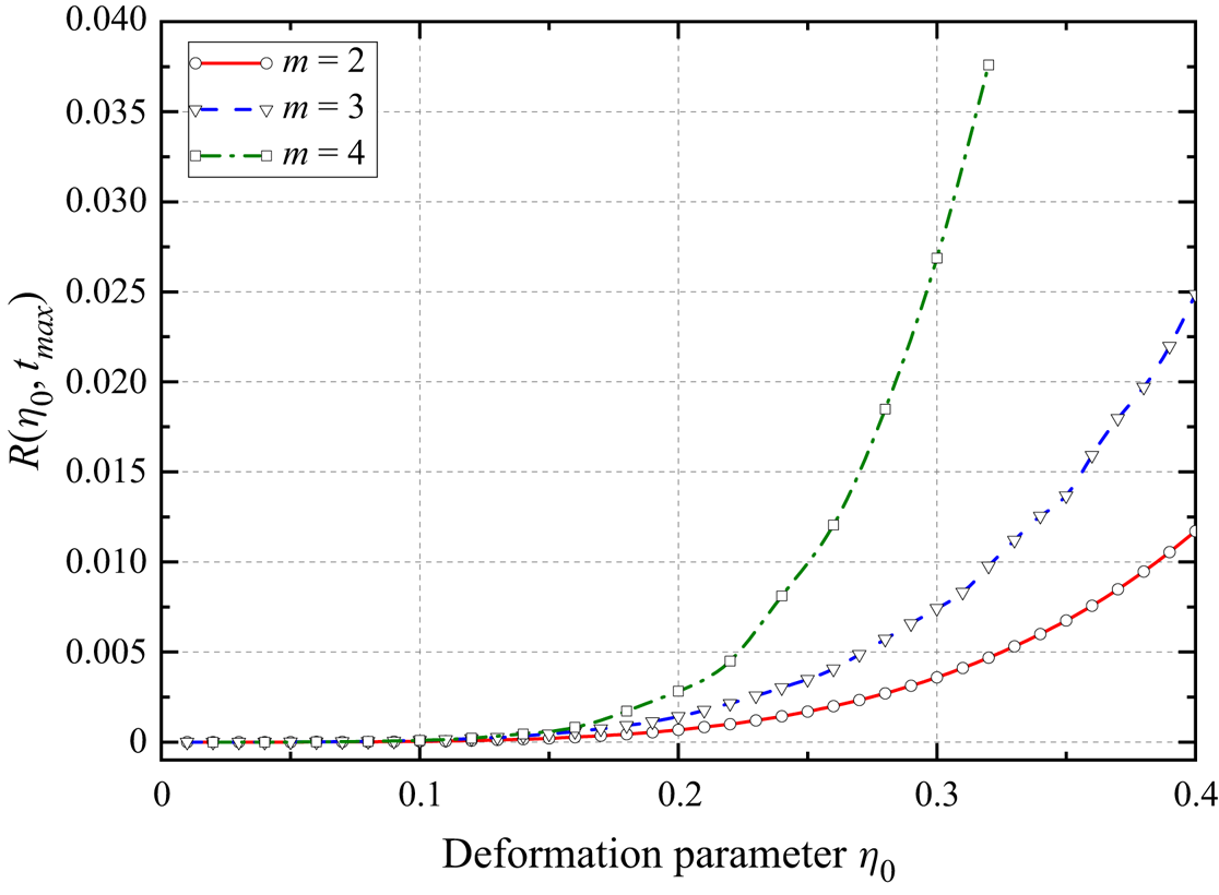
The values of  $R$ are all positive, oscillate in time and increase with
 $\eta _{0}$. Figure 2 presents the results for the modes of initial deformation
 $m=2, 3$ and
 $4$ at the instant of time
 $t = t_{max}$ of largest volume deviation. The relative volume deviation for the fundamental mode
 $m=2$ at the relatively large deformation
 $\eta _0 = 0.4$ is around 1 %, while for
 $m=3$ it is around
 $2.5\,\%$.
Maximum relative drop volume deviation for initial modes of deformation  $m =2$, 3 and 4 as a function of the deformation parameter
 $\eta _{0}$.

4.2. Deformed drop surface shapes
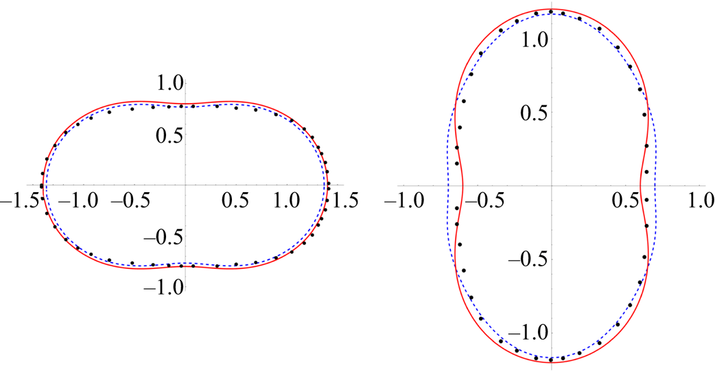
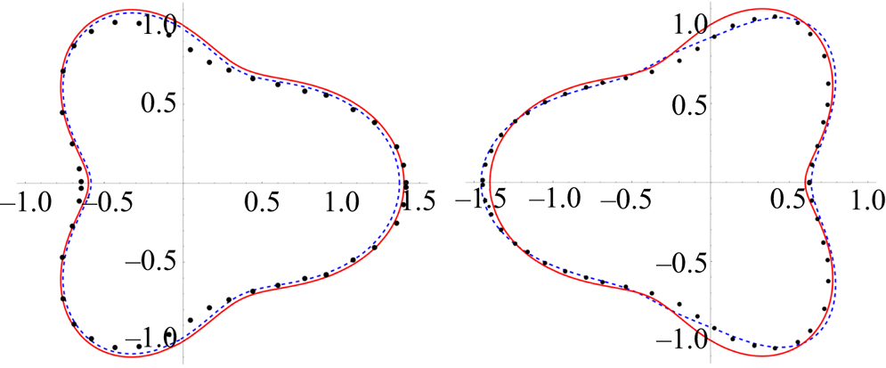
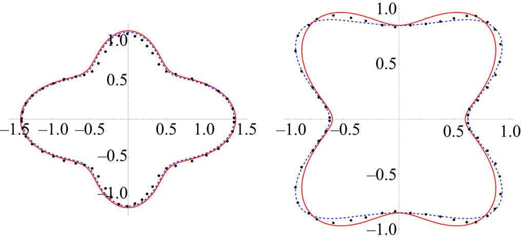
The results of the analysis include the deformed drop surface shapes up to third order. The results are validated against results from Tsamopoulos & Brown (Reference Tsamopoulos and Brown1983) in figures 3–5 for the initial deformation modes  $m =$
 $2$,
 $3$ and
 $4$. The drop shapes in these figures are turned by
 $90$ degrees against the sketch in figure 1, so that the axis of symmetry is horizontal. Every figure shows the results from the present WNLT to first order (Rayleigh) and to third order in states of maximum deformation. The deformation parameter
 $\eta _{0} = 0.4$, which corresponds to the shapes by Tsamopoulos & Brown (Reference Tsamopoulos and Brown1983) indicated in the figures by black dots for validation of the present results. The third-order results are in good agreement with the data by Tsamopoulos & Brown (Reference Tsamopoulos and Brown1983).
Maximum deformed prolate and oblate states of a drop for the initial deformation mode  $m=2$ with
 $\eta _{0}=0.4$, axisymmetric around the abscissa axis. Results include the WNLT of first order (——–, red) and third order (– – – –, blue). The third-order result from Tsamopoulos & Brown (Reference Tsamopoulos and Brown1983) is presented as black dots.

Figure 3 shows the drop shapes for the  $m = 2$ initial deformation, i.e. the prolate-to-oblate oscillation with a ratio, of drop length to width,
 $L/W =1.76$. The degrees of Legendre polynomials contributing to the field variables of second and third orders for various modes of initial deformation are listed in table 2. In the third-order approximation, we get the coefficient
 $\nu _{2}=-0.585187$ of the strained time coordinate. In the second-order approximation, our theory yields corrections to the frequency for initial deformation modes
 $m>2$ only.
Degrees of Legendre polynomials contributing to the solutions at second and third order for the modes of initial deformation  $m = 2,3,4$.

Figures 4 and 5 show the three- and four-lobed drop shapes in their states of maximum deformation. The results are in good agreement with Tsamopoulos & Brown (Reference Tsamopoulos and Brown1983). The degrees of the Legendre polynomials contributing to the third-order surface deformations for  $m=3$ given in table 2. They all have odd degrees, while for
 $m=4$ only the even degrees from
 $0$ to
 $12$ contribute. The third-order results follow the fundamental shapes of the first-order results, but at the rounded parts the radii of curvature at third order are smaller than for the linear shape. In the third-order calculation, the coefficient
 $\nu _{2}$ is
 $-0.988785$ and
 $-1.398515$ for the initial deformation modes
 $m=3$ and
 $m=4$, respectively. Tsamopoulos (Reference Tsamopoulos1990) determined frequency corrections which, in the present symbols, can be transcribed into the form
 $\nu = 1 + \nu _2 \epsilon ^{2}/2$, where
 $\nu _2 \approx -1.17037$ for
 $m=2$,
 $\nu _2 \approx -1.97757$ for
 $m=3$ and
 $\nu _2 \approx -2.79703$ for
 $m=4$. With account for the factor of
 $1/2$ in the frequency series, we see that the coefficients
 $\nu _2$ by Tsamopoulos (Reference Tsamopoulos1990) are identical to the present results.
Maximum deformed states of the drop for the initial deformation mode  $m=3$ with
 $\eta _{0}=0.4$, axisymmetric around the abscissa axis. Results include the WNLT of first order (——–, red) and third order (– – – –, blue). The third-order result from Tsamopoulos & Brown (Reference Tsamopoulos and Brown1983) is presented as black dots.

Maximum deformed states of the drop for the initial deformation mode  $m=4$ with
 $\eta _{0}=0.4$, axisymmetric around the abscissa axis. Results include the WNLT of first order (——–, red) and third order (– – – –, blue). The third-order result from Tsamopoulos & Brown (Reference Tsamopoulos and Brown1983) is presented as black dots.

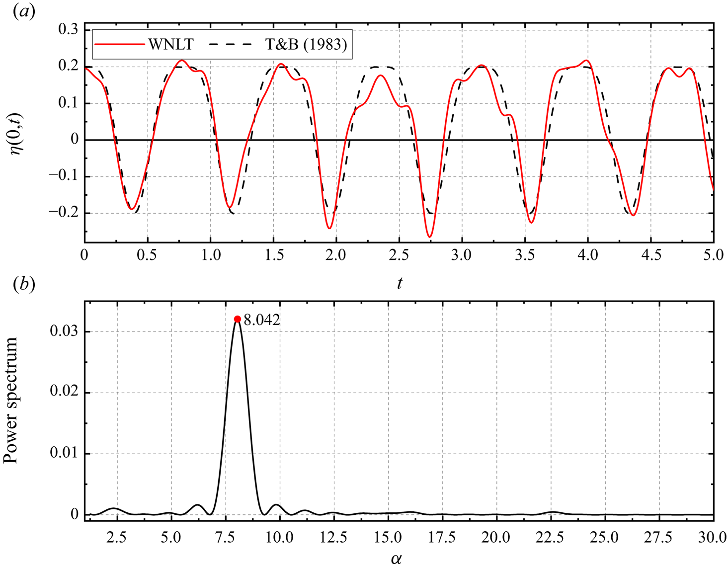
Figure 6(a) depicts the position of the drop's north pole relative to the undeformed state as a function of time for the initial deformation mode  $m = 4$ and
 $\eta _{0}=0.2$ in comparison with the third-order solution of Tsamopoulos & Brown (Reference Tsamopoulos and Brown1983). Figure 6(b) depicts the Fourier power spectrum of the oscillation from the present theory, showing the dominant mode together with others excited by mode coupling. The dominant frequency is smaller than the Rayleigh frequency of
 $8.485$ for
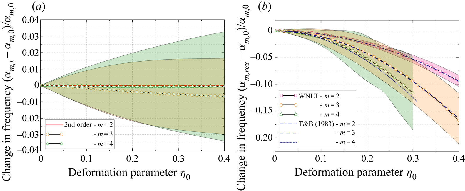
 $m=4$, as expected for the nonlinear oscillation. The influence of mode coupling on the drop dynamics increases with the deformation amplitude. The oscillations driven by initially higher modes experience stronger mode coupling; this will be discussed later. Another phenomenon seen in figure 6(a) is the quasi-periodicity of the motion as one consequence of mode coupling. Quasi-periodicity is excluded in Tsamopoulos & Brown (Reference Tsamopoulos and Brown1983) and Patzek et al. (Reference Patzek, Benner, Basaran and Scriven1991). This phenomenon explains the complex form of the deformation trace in time. The present results confirm the statement in Basaran (Reference Basaran1992) and Lundgren & Mansour (Reference Lundgren and Mansour1988) derived from numerical simulations that every third deformation amplitude peak is lower than the previous two. The frequency of the first oscillation agrees well with Tsamopoulos & Brown (Reference Tsamopoulos and Brown1983), but differs in the whole of the rest of the oscillatory motion. Quasi-periodicity makes the oscillation frequency vary in time. The frequency variation will be presented and discussed in the following subsection.
(a) Position of the drop north pole relative to the undeformed state as a function of time from the present WNLT, compared with Tsamopoulos & Brown (Reference Tsamopoulos and Brown1983). (b) Fourier power spectrum of the frequency for the oscillation in panel (a). The deformation parameter  $\eta _0 = 0.2$,
 $m=4$.

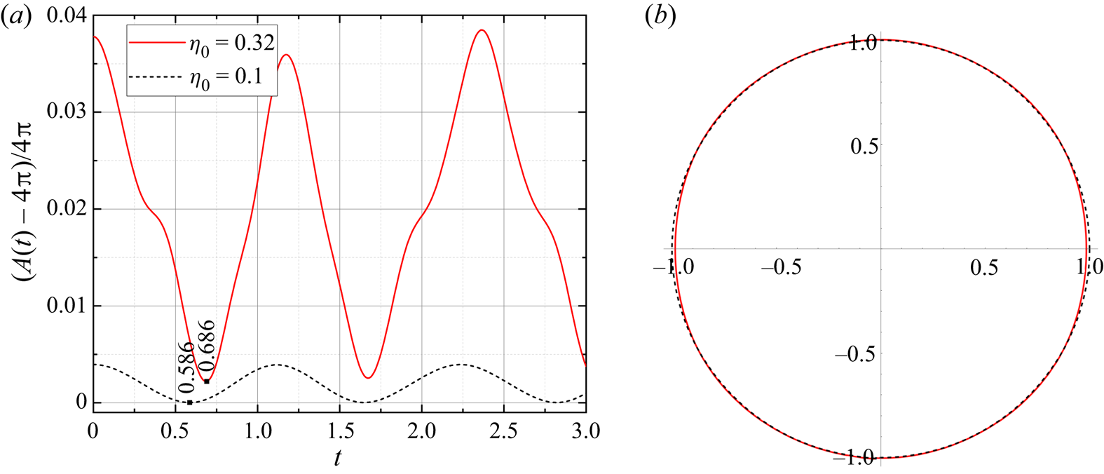
The change of the drop surface area in time due to the shape oscillations influences transport processes of momentum, as well as heat and mass. The effect is due to both the increase of the surface area, and the velocity fields inside and outside the drop surface, which influence gradients of velocity, temperature and species concentration. Figure 7(a) presents the relative surface area deviation from the spherical state for the initial deformation mode  $m=2$ as a function of time for the two different deformation parameters
 $\eta _{0}=0.1$ and
 $\eta _{0}=0.32$. In the maximum deformed state for
 $\eta _0 = 0.32$, the drop surface is larger than the spherical one by 3.8 % for
 $m=2$, and by 7 % and 11 % for
 $m=3$ and
 $m=4$, respectively (not shown). The trace of the calculated drop surface area for
 $\eta _{0}=0.1$ is sinusoidal, with minimum values equal to the non-dimensional surface area of the spherical shape. As the deformation parameter grows to
 $0.32$, however, the minimum surface areas increase, never becoming zero in the course of the oscillation. The appearance of the minimum surface area is delayed with increasing deformation parameter and, due to the quasi-periodicity of the motion, they appear irregularly in every period. The meridional section of the drop for
 $\eta _{0}=0.32$ at
 $t=0.686$, i.e. in the state of minimum drop surface area, is shown in comparison with the circular (minimum) shape for
 $\eta _{0}=0.1$ in figure 7(b). This result shows that drops oscillating nonlinearly at large amplitude never reach the spherical state during the oscillations (Patzek et al. Reference Patzek, Benner, Basaran and Scriven1991). This effect is not represented by the linear solution, and it appears for large initial deformations only. The minimum drop surface area as a function of the deformation parameter
 $\eta _0$ for the modes of initial deformation
 $m= 2, 3$ and
 $4$ is given in the supplementary material. The data show that, for all the modes, the minimum surface area increases according to the function
 $0.0142 (m\eta _0)^{4}$, which was found empirically.
(a) Relative deviation of the drop surface area from the sphere as a function of time. (b) Drop meridional section for  $\eta _{0}=0.32$ (——–, red) at minimum surface area, compared with the circular section for
 $\eta _{0}=0.1$ (– – – –), both at
 $m=2$.

4.3. Time scales of the drop shape oscillations
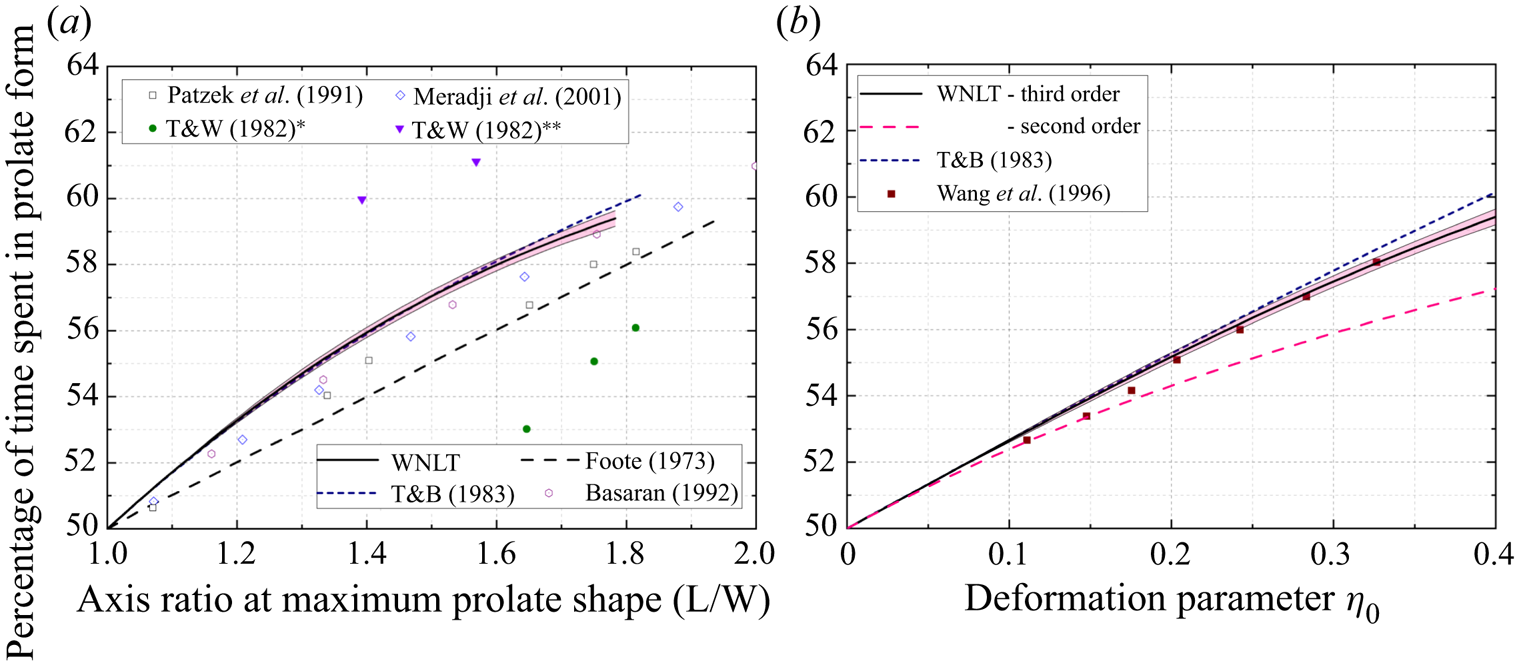
It is known as one nonlinear effect in drop shape oscillations that, for the prolate-oblate motions of mode  $m=2$, the drop spends more time in the prolate than in the oblate state of deformation. This effect is studied first in the present subsection, and results for
 $m=2$ are shown in figure 8. For ease of comparison with other literature, figure 8(a) shows the time per cent spent in the prolate form as a function of the drop aspect ratio, and 8(b) as a function of the deformation parameter
 $\eta _{0}$. The results by Tsamopoulos & Brown (Reference Tsamopoulos and Brown1983) are transcribed into the dependency on the deformation parameter by using their analytical solutions. The prolate times represented by the WNLT curves in figure 8(a,b) are determined from traces of the position of the drop north pole (
 $\theta = 0$) as a function of time, such as, for example, in figure 6(a). The times spent in the prolate state are measured for the first 10 oscillations of the traces from the third-order calculations. Due to the quasi-periodicity of the motion, the measured values differ in every oscillation. For every deformation parameter, therefore, the mean value and standard deviation of the time spent in the prolate state are calculated. The WNLT results are shown as solid lines for the mean and shaded areas for the standard deviation. The second-order results do not exhibit this phenomenon, so that their values are depicted by solid lines only. The data show that the present WNLT represents the time asymmetry of the
 $m=2$ drop shape oscillations. The results from the present WNLT are in excellent agreement with Tsamopoulos & Brown (Reference Tsamopoulos and Brown1983), but show slightly smaller excess times for strong deformations than the latter. This presentation of drop oscillation properties by mean values plus variance accounts for the fluctuations in time due to the quasi-periodic motion represented by the third-order approximation.
Percentage of the oscillation period in the  $m=2$ shape oscillations spent in the prolate shape (a) as a function of the aspect ratio
 $L/W$ of the drop at maximum deformation, and (b) as a function of the deformation parameter
 $\eta _{0}$. In panel (a), T&W(1982)* denotes experimental data by Trinh & Wang (Reference Trinh and Wang1982) for initial steady prolate drive, and T&W(1982)** for initial static prolate shape. Shaded areas represent the standard deviations.

Experimental results by Trinh & Wang (Reference Trinh and Wang1982), and numerical results by Foote (Reference Foote1973), Alonso (Reference Alonso1974), Patzek et al. (Reference Patzek, Benner, Basaran and Scriven1991), Basaran (Reference Basaran1992) and Meradji et al. (Reference Meradji, Lyubimova, Lyubimov and Roux2001), are shown in figure 8 for validation. The experimental data by Trinh & Wang (Reference Trinh and Wang1982) gives the percentage of time spent in prolate shapes by neutrally buoyant silicone oil and carbon tetrachloride mixture drops in distilled water. The shape oscillations were forced acoustically near the fundamental frequency. Turning the excitation off, the drop performed a free oscillation, and the oscillation frequency was measured. Calculation of the viscous correction due to the immiscible liquid–liquid system confirms the possibility of comparing the system with free drop shape oscillations in a vacuum. The viscous correction relates to the inviscid frequency derived by Prosperetti (Reference Prosperetti1980b) (given in figure 14 on p. 175 of that paper). It corrects the non-dimensional frequency with the viscosities of the inner and outer fluids having the same density. The corrections have also been made for the numerical data of Foote (Reference Foote1973) and Alonso (Reference Alonso1974). Chandrasekhar (Reference Chandrasekhar1959) states that the effect of the viscosity on the oscillation frequency is very small when the Ohnesorge number  $\mu / ( \sigma a \rho )^{1/2}$ is small. As pointed out by Tsamopoulos & Brown, from the data of Foote (Reference Foote1973) and Alonso (Reference Alonso1974) the Ohnesorge numbers of 1/35.4 and 1/3.3 follow, respectively, which both satisfy the condition. Further numerical work investigating the time evolution of small-viscosity drop oscillations (
 $Oh=0.01$) is due to Basaran (Reference Basaran1992) and Meradji et al. (Reference Meradji, Lyubimova, Lyubimov and Roux2001). Patzek et al. (Reference Patzek, Benner, Basaran and Scriven1991) studied numerically oscillations of free inviscid liquid drops. Their results are also included in the present comparison. The percentage of time spent in the prolate form of the two-lobed oscillations from the latter three studies fits in the region between our inviscid WNLT and the small-viscosity results by Foote (Reference Foote1973). Figure 8(a), presenting data by Trinh & Wang (Reference Trinh and Wang1982), shows that the initial state of the drop – steady prolate drive or static prolate shape – has an influence on mode coupling. Therefore, the time asymmetry found in the oscillatory motion is quite different.
The method of Trinh & Wang (Reference Trinh and Wang1982) for determining the time spent in the prolate form and the oscillation frequency for different deformation amplitudes was applied by Wang et al. (Reference Wang, Anilkumar and Lee1996) to drops acoustically positioned in a microgravity environment. The data for a glycerin–water drop with  $Oh=0.0125$ are extracted using a central averaging scheme to eliminate the role of viscosity in nonlinear effects. Low-viscosity results may be compared with the inviscid case only if
 $Oh \ll 0.1$, which is the case in the experiments reported by Trinh & Wang (Reference Trinh and Wang1982). Figure 8(b) shows comparisons of the excess times from the present second- and third-order solutions with the results by Tsamopoulos & Brown (Reference Tsamopoulos and Brown1983) and Wang et al. (Reference Wang, Anilkumar and Lee1996). For small deformation parameters
 $\eta _0 < 0.15$, the present third-order results collapse with the data by Tsamopoulos & Brown (Reference Tsamopoulos and Brown1983). For higher deformation parameters, these results represent the data by Wang et al. (Reference Wang, Anilkumar and Lee1996) very well.
Another nonlinear effect in drop shape oscillations is a decrease of the oscillation frequency with increasing drop deformation. The WNLT represents this effect. Figure 9(a) shows the relative decrease of the oscillation frequency below the Rayleigh value  $\alpha _{2,0}$ as a function of the maximum aspect ratio
 $L/W$ of the drop shape reached in the oscillations for the initial deformation mode
 $m = 2$. Figure 9(b) shows data as a function of the deformation parameter
 $\eta _{0}$ for ease of comparison with other literature. The oscillation frequencies represented by the WNLT curves in figures 9(a) and 9(b) are determined from traces of the position of the drop north pole (
 $\theta = 0$) as a function of time, such as, for example, in figure 6(a). The period length found in these data determines the resultant angular oscillation frequency termed
 $\alpha _{2,res}$ on the ordinate axis of figure 9. For every deformation parameter, the period lengths are measured for a set of 10 oscillations on the trace. Alternatively, the surface deformation was plotted as a function of the stretched time coordinate
 $\tau$, which was introduced to suppress secular terms in the solutions of a differential equation arising in the theoretical analysis. Determining the period length from these traces, a frequency decrease or increase is found, which is due to mode coupling only, arising from the various time dependencies of the nonlinear terms in the governing equations and boundary conditions for the second- and third-order approximations. Three different WNLT results are presented: the frequency decrease for the first and second oscillations of each trace, with the solid lines depicting the resultant values, and the dashed lines the contributions from mode coupling only. The mode coupling causes quasi-periodicity, which is visible from the variation of the oscillation frequency. The resultant values variation is quantified by the standard deviation, represented by the shaded areas. Subtracting the mode coupling result from the resultant values yields the means, which collapse with the data by Tsamopoulos & Brown (Reference Tsamopoulos and Brown1983). The third results from the WNLT, depicted by solid lines with square symbols, represent the mean values from each set of 10 oscillations analysed. The shape of the resultant frequency decrease for
 $m=2$ is concave, which is due to the quadratic form of the strained time coordinate. For the same mode, the mode coupling which is manifested in appearance of shaded area is weak, and the mean results collapse perfectly with the data by Tsamopoulos & Brown (Reference Tsamopoulos and Brown1983). The results of the WNLT including the standard deviation collapse with the data by Foote (Reference Foote1973) and by Patzek et al. (Reference Patzek, Benner, Basaran and Scriven1991) and follow the same quadratic shape.
Decrease of the angular frequency for the  $m=2$ oscillation (a) as a function of the drop aspect ratio
 $L/W$, and (b) as a function of the deformation parameter
 $\eta _{0}$ for comparison with different literature. Shaded areas represent the standard deviations.

Figure 9(b) shows inviscid numerical results by Dürr & Siekmann (Reference Dürr and Siekmann1987), Becker et al. (Reference Becker, Hiller and Kowalewski1991), Wang et al. (Reference Wang, Anilkumar and Lee1996) and Smith (Reference Smith2010), and the classical results from Tsamopoulos & Brown (Reference Tsamopoulos and Brown1983) transcribed into the dependency on the deformation parameter by using their analytical solutions. Smith uses different time scales and a formal perturbation scheme to determine original modulation equations. Using two ordinary differential equations of the conservation of energy and the averaged projection of the Navier–Stokes equations onto the vorticity vector, the author derives expressions for the drop surface deformation. The analytical work by Becker et al. (Reference Becker, Hiller and Kowalewski1991) studies the motion of an inviscid, incompressible droplet in a vacuum, while Dürr & Siekmann (Reference Dürr and Siekmann1987) carried out numerical simulations using the boundary-integral technique. All the three investigations confirmed a decrease of the oscillation frequency with increasing deformation amplitude as a nonlinear characteristic of the  $m = 2$ oscillations. The present WNLT data, including the variations due to mode coupling, collapses with all the compared data.
After this analysis of excess time and frequency decrease for the initial deformation mode  $m=2$, we study higher modes of initial deformation. Figure 10 depicts the percentage of the oscillation period the drop north pole (
 $\theta = 0$) spends at a larger distance from the drop centre than in the spherical state for the modes
 $m=2, 3$ and
 $4$. These north pole positions indicate an elongation of the drop in the direction of the symmetry axis. For
 $m=2$, this shape is defined as prolate. Figures 10(a) and 10(b) show the mean values and standard deviations of the percentage of the oscillation period spent in elongated shape for second and third order of approximation, respectively. The lines represent the mean values, and the shaded areas the standard deviations as functions of the deformation parameter
 $\eta _0$ for every
 $m$. The data are deduced from the first 10, eight and six oscillations for the initial deformation modes
 $m=2, 3$ and
 $4$, respectively. The number of oscillations in the set is smaller for the higher initial deformation modes, since at third order of approximation the surface deformation trace with time becomes more and more complicated with increasing
 $\eta _0$, thus making it impossible to identify period lengths. For this reason the data for the initial mode
 $m=4$ runs to
 $\eta _{0}=0.3$ only. Figures 10(a) and 10(b) show that the excess time increases with the mode of initial deformation, with the deformation parameter
 $\eta _0$, and with the order of approximation. An important difference between the present WNLT and Tsamopoulos & Brown (Reference Tsamopoulos and Brown1983) is the quasi-periodicity of the motion at stronger deformation, which is represented by the present theory. Oscillations of the fundamental mode exhibit a weak mode coupling. For
 $m=2$, in figure 10(a) the data from both theories at second-order approximation show no quasi-periodicity. From this finding we conclude that quasi-periodicity is a third-order effect for
 $m=2$, but it is a second-order effect for the higher modes of initial deformation.
Percentage of the oscillation period the drop spends in a shape elongated along the symmetry axis as a function of the deformation parameter  $\eta _{0}$ for oscillations with
 $m = 2, 3$ and
 $4$. Mean value and standard deviation including (a) the second-order and (b) the third-order approximation, compared with Tsamopoulos & Brown (Reference Tsamopoulos and Brown1983).

A comparison of the frequency decrease as a function of  $\eta _{0}$ between the modes
 $m=2, 3$ and
 $4$ is shown in figure 11. Figures 11(a) and 11(b) show the mean values and standard deviations of the relative frequency change for second and third order of approximation, respectively. The data are deduced from the first 10, eight and six oscillations for
 $m=2, 3$ and
 $4$, respectively. We also present the results by Tsamopoulos & Brown (Reference Tsamopoulos and Brown1983) in figure 11(b) for comparison. For
 $m=2$, the frequency does not change with the deformation parameter in the second-order approximation, thus requiring the theory to be taken to third order to see this effect for this mode. The mean relative frequency change for
 $m\geq 3$ at second order (figure 11a) is also close to zero. However, the frequency fluctuates in time, as represented by the shaded areas. The fluctuations increase with the mode of initial deformation and with the deformation parameter. We explain this behaviour with the modes excited already in the second-order approximation, which are absent at
 $m=2$. Since the number of excited modes increases with increasing initial deformation mode, as shown in table 2, the frequency fluctuations also increase with this mode. As a consequence, the quasi-periodicity is enhanced with increasing mode of initial deformation and produces stronger frequency fluctuations, which for
 $m=4$ start to oscillate. The mean relative frequency decreases agree well with Tsamopoulos & Brown (Reference Tsamopoulos and Brown1983).
Decrease of the angular frequency as a function of the deformation parameter  $\eta _{0}$ for oscillations with
 $m = 2, 3$ and
 $4$. Mean value and standard deviation of the relative decrease of (a)
 $\alpha _{m,i}$ at second, and (b)
 $\alpha _{m,res}$ at third order of approximation compared with Tsamopoulos & Brown (Reference Tsamopoulos and Brown1983).

5. Conclusions
A weakly nonlinear analysis of shape oscillations of an inviscid, axisymmetric liquid drop in a vacuum was performed. The components of the velocity vector field, the pressure and the drop shape are expanded in power series of a small deformation parameter  $\eta _0$, yielding sets of equations of motion with their boundary and initial conditions corresponding to different orders of the expansion. The analysis is taken to third order. Secular solutions for the surface deformation, appearing at second and third orders of approximation, are eliminated using a strained time coordinate. In the special case of the two-lobed initial deformation mode
 $m=2$, an additional pair of secular terms arises, which are suppressed by setting related coefficients in the series expansions to zero.
The first-order solution is the linear one known from Rayleigh (Reference Rayleigh1879). The second and third orders represent the nonlinear influences from the first order and from the first and second orders, respectively. Due to the truncated power series representing the drop shape, the non-dimensional drop volume deviates from the value of  $4 \pi / 3$. For the two- and three-lobed deformation modes
 $m=2$ and
 $m=3$, the relative deviation at large deformations up to
 $\eta _{0} = 0.4$ is around
 $1\,\%$ and
 $2.5\,\%$, respectively. The applied weakly nonlinear approach proves capable of representing the quasi-periodic motions induced by nonlinearity for increasing deformation amplitude, which were found by other authors in numerical simulations. Fourier frequency power spectra reveal frequencies induced by mode coupling. The deviation from the spherical shape leads to an increase of the drop surface area. The surface area increase is stronger for higher deformation parameters. For fixed
 $\eta _{0}=0.4$, the surface area increases are around
 $6\,\%$,
 $10\,\%$ and
 $14\,\%$ for the initial modes
 $m=2, 3$ and
 $4$, respectively. As nonlinear effects, an asymmetry in the times the drop spends in the oblate and prolate deformed states, and a decrease of the oscillation frequency, are known for the mode
 $m = 2$. The present theory represents these effects correctly, in agreement with existing experimental and theoretical literature, and extends the results to the multi-lobed deformation modes
 $m=3$ and
 $m=4$. The frequency decrease is found to be a third-order effect for the fundamental deformation mode
 $m=2$. For all higher-order modes of deformation, the frequency decrease is seen in the second-order approximation already. Due to the quasi-periodic oscillatory motion, both the time asymmetry and the frequency vary in time.
The present results reveal the detailed time behaviour of drops in nonlinear shape oscillations. The study goes beyond the classical literature in that it represents the influence of the coupling of modes excited by the mode of initial deformation on the time behaviour of the oscillations. The analysis up to third order represents the quasi-periodic nature of the oscillations, which is due to the interaction between the various modes. As one consequence of this, the analytically determined drop surface area shows that drops in nonlinear oscillations at strong deformations never reach the spherical state, thus exhibiting a resultant surface area increase above the value of the sphere. The related velocity field in the drop influences the transport of momentum, heat and mass across the drop surface. The motion of the drop surface induces motion of the gas phase, which influences transfer processes. The results are relevant for applications in the modelling of transport processes across the oscillating drop surface, such as the quantification of the drag coefficient, as well as the rates of heat and mass transfer. Applications in production techniques such as containerless materials processing on the basis of single drops and in-air microfluidics have benefit from the results.
Supplementary material
Supplementary material are available at https://doi.org/10.1017/jfm.2021.568.
Acknowledgements
Valuable discussions with Professor J. Tsamopoulos at the University of Patras (GR) are gratefully acknowledged. We acknowledge gratefully valuable advice from Professor J. Eggers at the University of Bristol (UK).
Funding
Financial support of this research project by the Austrian Science Fund (FWF) through project number I3326-N32 in the DACH framework is gratefully acknowledged.
Declaration of interests
The authors report no conflict of interest.