1 Introduction
The aim of this paper is to perform a linear stability analysis of a two-layer plane Couette flow of two immiscible fluid layers with different densities, viscosities and thicknesses, bounded by two infinite parallel plates moving at a constant relative velocity to each other, with an insoluble surfactant monolayer along the interface and in the presence of gravity.
It is well known that the presence of surfactant can modify the stability properties of fluid flows (e.g. Edwards, Brenner & Wasan (Reference Edwards, Brenner and Wasan1991)). Before the work of Frenkel & Halpern (Reference Frenkel and Halpern2002) (hereafter referred to as FH) and Halpern & Frenkel (Reference Halpern and Frenkel2003) (from now on referred to as HF), the cases of flows with insoluble surfactants were limited to single-fluid flows with a free surface (e.g. Whitaker (Reference Whitaker1964), Anshus & Acrivos (Reference Anshus and Acrivos1967), Otis et al. (Reference Otis, Johnson, Pedley and Kamm1993), De Wit, Gallez & Christov (Reference De Wit, Gallez and Christov1994)) or multi-fluid systems without a base flow (e.g. Kwak & Pozrikidis (Reference Kwak and Pozrikidis2001)). In those cases, the influence of insoluble surfactants was shown to be stabilizing or neutral.
In contrast, FH and HF showed that under certain conditions, an insoluble surfactant monolayer at the interface between two fluid layers may have a destabilizing effect on the viscosity-dominated flows. This instability occurs provided there is a non-zero shear at the interface (which is not the case for the before mentioned single-fluid flows with a free interface or stagnant multi-fluid systems). Unlike the well-known instability of two viscous fluids with different viscosities (Yih Reference Yih1967), this surfactant instability does not require inertia for its existence. In cylindrical flows, such as core-annular flows, this instability has to compete with the capillary instability of the cylindrical interface which is always present even without surfactants (see e.g. Bassom, Blyth & Papageorgiou (Reference Bassom, Blyth and Papageorgiou2012) and references therein). In contrast, for planar flows, the interfacial surfactant can be the sole source of instability. Regarding horizontal channel flows with a surfactant-laden sheared interface, the inertialess surfactant instability was studied in a number of papers. Blyth & Pozrikidis (Reference Blyth and Pozrikidis2004b ) confirmed the inertialess surfactant instability of FH and HF, and performed nonlinear numerical simulations on short computational domains. Pozrikidis (Reference Pozrikidis2004), Blyth & Pozrikidis (Reference Blyth and Pozrikidis2004a ) and Frenkel & Halpern (Reference Frenkel and Halpern2005) examined the influence of inertia on this type of instability. Pozrikidis & Hill (Reference Pozrikidis and Hill2011) considered a two-layer Couette channel flow and studied the linear stability with the emphasis on different asymptotic limits such as the one of the infinite thickness ratio and also the limit of infinitesimally short waves which they interpreted as the cases of one or two semi-infinite fluids, respectively. Frenkel & Halpern (Reference Frenkel and Halpern2006) and Bassom, Blyth & Papageorgiou (Reference Bassom, Blyth and Papageorgiou2010) studied the nonlinear stability of two-fluid channel flow with surfactants for the long-wave disturbances assuming that one layer is much thinner than the other (at the leading order of the small thickness ratio, so that the results do not depend on the thickness ratio). The latter paper took into account the influence of the thick layer disturbances, assuming their wavelengths to be large, which was relaxed in Kalogirou, Papageorgiou & Smyrlis (Reference Kalogirou, Papageorgiou and Smyrlis2012). Kalogirou & Papageorgiou (Reference Kalogirou and Papageorgiou2016) extended the work of Kalogirou et al. (Reference Kalogirou, Papageorgiou and Smyrlis2012) by including the effects of inertia in the thick layer and three-dimensional disturbances. Frenkel & Halpern (Reference Frenkel and Halpern2017) added gravity to the long-wave stability analysis of channel flows with interfacial surfactants of FH (formulated in a manner suggested by Wei (Reference Wei2005)). Since in the absence of surfactants gravity can be either stabilizing or destabilizing depending on the flow parameters, the interaction of the Rayleigh–Taylor instability with the surfactant instability leads to interesting phenomena, in particular in nonlinear regimes. Kalogirou (Reference Kalogirou2018) extended the work of Kalogirou & Papageorgiou (Reference Kalogirou and Papageorgiou2016) by including gravity in addition to the effects of surfactants and the thick layer inertia (for two-dimensional disturbances).
The instability of two-layer channel flows with soluble surfactants was studied recently by Rickett et al. (Reference Rickett, Penfold, Blyth, Purvis and Cooker2015) and Picardo, Radhakrishna & Pushpavanam (Reference Picardo, Radhakrishna and Pushpavanam2016). They made the limiting assumption of instantaneous adsorption/desorption of the surfactant at the interface (which, in particular, implies that the internal transport of interfacial surfactant is negligible). In such models, the instability requires a non-zero flux of the surfactant across the channel in the base state (with the walls being permeable to the surface active solute), in which case it can be unstable even for a zero base flow (Sternling & Scriven Reference Sternling and Scriven1959). The case of insoluble surfactant, never leaving the interface, implies a completely different, infinitely slow, adsorption/desorption kinetics. The latter model cannot be obtained as a parametric limit of such soluble surfactant models as those mentioned above (Picardo et al. Reference Picardo, Radhakrishna and Pushpavanam2016).
The paper by Frenkel & Halpern (Reference Frenkel and Halpern2017) was confined to long-wave disturbances and based on the well-known lubrication approximation. By contrast, in the present work, the linear stability analysis includes disturbances of arbitrary wavenumbers, which is more challenging. It can also be regarded as an extension of HF, who considered arbitrary wavenumbers, but did not include the effects of gravity, which are incorporated in the present work. As was indicated in Frenkel & Halpern (Reference Frenkel and Halpern2017), one can expect a rich landscape of stability properties, especially since there are two active normal modes of infinitesimal disturbances corresponding to the presence of two interfacial functions: the interface displacement function and the interfacial surfactant concentration (FH, HF). Since the growth rates of the normal modes are the real parts of the increments which are shown to satisfy a (complex) quadratic equation, they are available as explicit functions for all wavenumbers, and in many instances numerical results may enjoy analytic (asymptotic) corroboration.
The inclusion of gravity leads to different new phenomena. This investigation started in Schweiger (Reference Schweiger2013). The present paper constitutes the first part of our work and deals with long-wave instability regimes, defined as those having a single interval of unstable wavenumbers (not necessarily all small) which has zero as its left endpoint. The second part (Frenkel, Halpern & Schweiger Reference Frenkel, Halpern and Schweiger2019; below, referred to as ‘Part 2’), focuses on the mid-wave regimes (HF), defined as those having a finite interval of unstable wavenumbers bounded away from zero. Both parts are presented together in more detail in Frenkel, Halpern & Schweiger (Reference Frenkel, Halpern and Schweiger2018).
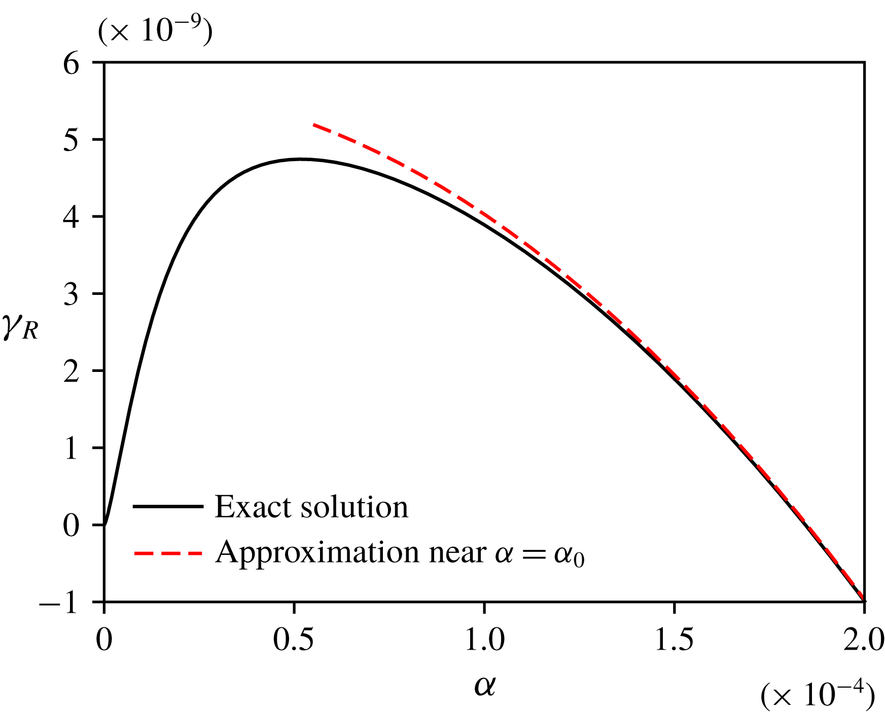
In § 2, the stability problem is formulated. In § 3, the dispersion equation is obtained. The long-wave stability properties for finite wavenumbers, which were beyond the scope of Frenkel & Halpern (Reference Frenkel and Halpern2017), are considered in § 4, while in § 5 we deal with arbitrary wavelengths. Finally, § 6 contains discussion and concluding remarks. The mathematical considerations concerning the existence of the two branches of the growth rate as continuous functions of the wavenumber and the system parameters can be found in the Appendix.
2 Stability problem formulation
The general framework and governing equations of the problem were given before (see Schweiger Reference Schweiger2013; Frenkel & Halpern Reference Frenkel and Halpern2017) and are as follows. Two immiscible Newtonian fluid layers with different densities, viscosities and thicknesses are bounded by two infinite horizontal plates, a distance
 $d=d_{1}+d_{2}$
apart (see figure 1 for the definition sketch of the Couette flow which we study here). The unperturbed liquid–liquid interface is located at
 $z^{\ast }=0$
, the top plate at
 $z^{\ast }=d_{2}$
and the bottom plate at
 $z^{\ast }=-d_{1}$
, where
 $z^{\ast }$
-axis is the spanwise, vertical coordinate. (The symbol
 $^{\ast }$
indicates a dimensional quantity.) The frame of reference is fixed at the liquid–liquid interface. The unperturbed Couette flow has only the horizontal component, which is linear in
 $z^{\ast }$
, and changes from zero at the interface to
 $-U_{1}^{\ast }$
at the bottom plate and
 $U_{2}^{\ast }$
at the top plate, where
 $U_{1}^{\ast }+U_{2}^{\ast }=U^{\ast }$
, the velocity of the top plate relative to the bottom plate. The base surfactant concentration is uniform along the base flat interface. Once disturbed, the surfactant concentration is no longer uniform and, along with the interfacial deflection, depends on
 $x^{\ast }$
and
 $t^{\ast }$
, where
 $x^{\ast }$
is the horizontal coordinate and
 $t^{\ast }$
is the time variable. The infinitesimal disturbances may grow under the action of the Marangoni and/or gravity forces (Frenkel & Halpern Reference Frenkel and Halpern2017).
In HF, for the same system but without gravity effects, we have established an appropriately modified Squire’s theorem (see appendix C there. For other cases of multilayer flows see Hesla, Prankch & Preziosi (Reference Hesla, Prankch and Preziosi1986), Joseph & Renardy (Reference Joseph and Renardy1993)). It is easy to see that the same theorem holds with gravity effects present. Indeed the only modification in the disturbance equations (C2)–(C12) in HF is adding the term
 $-Boh$
to the right-hand side of the normal stress balance equation (C10) where
 $Bo$
is an appropriate Bond number. (Its exact definition appears at the end of this section.) Therefore, the theorem formulation is as before with the same transformation from a three-dimensional solution to a two-dimensional one, which depends on the streamwise coordinate only, with the additional transformation equation
 $\widehat{Bo}=Bo$
which would be added to (C16). In view of this, we confine our consideration to two-dimensional perturbed flows (in the
 $x^{\ast }z^{\ast }$
-plane).
Definition sketch of a two-layer Couette flow of two horizontal liquid layers with different thicknesses
 $d_{i}$
(
 $i=1$
for the bottom layer and
 $i=2$
for the top layer), viscosities
 $\unicode[STIX]{x1D707}_{i}$
and densities
 $\unicode[STIX]{x1D70C}_{i}$
. The disturbed interface is located at
 $z^{\ast }=\unicode[STIX]{x1D702}^{\ast }(x^{\ast },t^{\ast })$
, and is coated by an insoluble surfactant monolayer indicated by dots. Gravity acts in the spanwise direction.

The governing equations for this problem are given, in both dimensional and dimensionless forms, elsewhere (see, for example, Frenkel & Halpern (Reference Frenkel and Halpern2017) and references therein). We use the following notations (with
 $j=1$
for the bottom liquid layer and
 $j=2$
for the top liquid layer):
 $\unicode[STIX]{x1D70C}_{j}$
is the density;
 $\boldsymbol{v}_{j}^{\ast }=(u_{j}^{\ast },w_{j}^{\ast })$
is the fluid velocity vector with horizontal component
 $u_{j}^{\ast }$
and vertical component
 $w_{j}^{\ast }$
;
 $p_{j}^{\ast }$
is the pressure;
 $\unicode[STIX]{x1D707}_{j}$
is the viscosity; and
 $g$
is the gravity acceleration.
We assume the dependence of surface tension
 $\unicode[STIX]{x1D70E}^{\ast }$
on the surfactant concentration
 $\unicode[STIX]{x1D6E4}^{\ast }$
to be given by the Langmuir isotherm relation (e.g. Edwards et al.
Reference Edwards, Brenner and Wasan1991). For small disturbances,
 $$\begin{eqnarray}\displaystyle \unicode[STIX]{x1D70E}^{\ast }=\unicode[STIX]{x1D70E}_{0}-E(\unicode[STIX]{x1D6E4}^{\ast }-\unicode[STIX]{x1D6E4}_{0}), & & \displaystyle\end{eqnarray}$$
where
 $\unicode[STIX]{x1D70E}_{0}$
is the base surface tension corresponding to the base surfactant concentration
 $\unicode[STIX]{x1D6E4}_{0}$
and the known constant
 $E:=-(\unicode[STIX]{x2202}\unicode[STIX]{x1D70E}^{\ast }/\unicode[STIX]{x2202}\unicode[STIX]{x1D6E4}^{\ast })|_{\unicode[STIX]{x1D6E4}^{\ast }=\unicode[STIX]{x1D6E4}_{0}}$
is the elasticity parameter.
We use the following dimensionless variables:
 $$\begin{eqnarray}\displaystyle \left.\begin{array}{@{}c@{}}\displaystyle (x,z,\unicode[STIX]{x1D702})=\frac{(x^{\ast },z^{\ast },\unicode[STIX]{x1D702}^{\ast })}{d_{1}},\quad t=\frac{t^{\ast }}{d_{1}\unicode[STIX]{x1D707}_{1}/\unicode[STIX]{x1D70E}_{0}},\quad \boldsymbol{v}_{j}=(u_{j},w_{j})=\frac{(u_{j}^{\ast },w_{j}^{\ast })}{\unicode[STIX]{x1D70E}_{0}/\unicode[STIX]{x1D707}_{1}},\\ \displaystyle p_{j}=\frac{p_{j}^{\ast }}{\unicode[STIX]{x1D70E}_{0}/d_{1}},\quad \unicode[STIX]{x1D6E4}=\frac{\unicode[STIX]{x1D6E4}^{\ast }}{\unicode[STIX]{x1D6E4}_{0}},\quad \unicode[STIX]{x1D70E}=\frac{\unicode[STIX]{x1D70E}^{\ast }}{\unicode[STIX]{x1D70E}_{0}}.\end{array}\right\} & & \displaystyle\end{eqnarray}$$
As in Frenkel & Halpern (Reference Frenkel and Halpern2017), the dimensionless velocity field of the basic Couette flow, with a flat interface,
 $\unicode[STIX]{x1D702}=0$
, uniform surface tension,
 $\bar{\unicode[STIX]{x1D70E}}=1$
, and corresponding surfactant concentration,
 $\bar{\unicode[STIX]{x1D6E4}}=1$
(where the over-bar indicates a base quantity), is
 $$\begin{eqnarray}\displaystyle \bar{u}_{1}(z)=sz,\quad \bar{w}_{1}=0,\quad \text{and}\quad \bar{p}_{1}=-Bo_{1}z\quad \text{for }-1\leqslant z\leqslant 0, & & \displaystyle\end{eqnarray}$$
 $$\begin{eqnarray}\displaystyle \bar{u}_{2}(z)=\frac{s}{m}z,\quad \bar{w}_{2}=0,\quad \text{and}\quad \bar{p}_{2}=-Bo_{2}z\quad \text{for }0\leqslant z\leqslant n, & & \displaystyle\end{eqnarray}$$
where
 $Bo_{j}:=\unicode[STIX]{x1D70C}_{j}gd_{1}^{2}/\unicode[STIX]{x1D70E}_{0}$
is the Bond number of the layer
 $j$
,
 $m=\unicode[STIX]{x1D707}_{2}/\unicode[STIX]{x1D707}_{1}$
is the ratio of the viscosities, and
 $n=d_{2}/d_{1}$
is the ratio of the thicknesses. The constant
 $s$
represents the base interfacial shear rate of the bottom layer,
 $s=D\bar{u}_{1}(0)$
, where
 $D=\text{d}/\text{d}z$
, and is used to characterize the flow instead of the relative velocity of the plates. It is straightforward to establish that
 $U=\unicode[STIX]{x1D707}_{1}U^{\ast }/\unicode[STIX]{x1D70E}_{0}=s(1+n/m)$
. The disturbed state with small deviations (indicated by the tilde,
 $^{{\sim}}$
) from the base flow is given by
 $$\begin{eqnarray}\displaystyle \unicode[STIX]{x1D702}=\tilde{\unicode[STIX]{x1D702}},\quad u_{j}=\bar{u}_{j}+\tilde{u} _{j},\quad w_{j}=\tilde{w}_{j},\quad p_{j}=\bar{p}_{j}+\tilde{p}_{j},\quad \unicode[STIX]{x1D6E4}=\bar{\unicode[STIX]{x1D6E4}}+\tilde{\unicode[STIX]{x1D6E4}}. & & \displaystyle\end{eqnarray}$$
The normal modes are disturbances of the form
 $$\begin{eqnarray}\displaystyle (\tilde{\unicode[STIX]{x1D702}},\tilde{u} _{j},\tilde{w}_{j},\tilde{p}_{j},\tilde{\unicode[STIX]{x1D6E4}})=[h,\hat{u} _{j}(z),{\hat{w}}_{j}(z),\hat{f}_{j}(z),G]\text{e}^{\text{i}\unicode[STIX]{x1D6FC}x+\unicode[STIX]{x1D6FE}t}, & & \displaystyle\end{eqnarray}$$
where
 $\hat{u} _{j}(z)$
,
 ${\hat{w}}_{j}(z)$
and
 $\hat{f}_{j}(z)$
are the complex amplitudes that depend on the depth,
 $\unicode[STIX]{x1D6FC}$
is the wavenumber of the disturbance,
 $G$
is the constant amplitude of
 $\tilde{\unicode[STIX]{x1D6E4}}$
(
 $G=\hat{\unicode[STIX]{x1D6E4}}$
),
 $h$
is the constant amplitude of
 $\tilde{\unicode[STIX]{x1D702}}$
(
 $h=\hat{\unicode[STIX]{x1D702}}$
) and
 $\unicode[STIX]{x1D6FE}$
is the increment,
 $\unicode[STIX]{x1D6FE}=\unicode[STIX]{x1D6FE}_{R}+\text{i}\unicode[STIX]{x1D6FE}_{I}$
. The stability of the flow depends on the sign of the growth rate
 $\unicode[STIX]{x1D6FE}_{R}$
: if
 $\unicode[STIX]{x1D6FE}_{R}>0$
for some normal modes then the system is unstable; and if
 $\unicode[STIX]{x1D6FE}_{R}<0$
for all normal modes then the system is stable. The linearized governing equations for the disturbances translate into the following system for the normal-mode amplitudes (see Frenkel & Halpern (Reference Frenkel and Halpern2017) and references therein for the omitted details). The continuity equation becomes
 $$\begin{eqnarray}\displaystyle \hat{u} _{j}=\frac{\text{i}}{\unicode[STIX]{x1D6FC}}D{\hat{w}}_{j}. & & \displaystyle\end{eqnarray}$$
Eliminating the pressure disturbances from the horizontal and vertical components of the momentum equations with neglected inertia yields the well-known Orr–Sommerfeld equations, here for the vertical velocity disturbances,
 $$\begin{eqnarray}\displaystyle m_{j}(D^{2}-\unicode[STIX]{x1D6FC}^{2})^{2}{\hat{w}}_{j}=0, & & \displaystyle\end{eqnarray}$$
where
 $m_{j}:=\unicode[STIX]{x1D707}_{j}/\unicode[STIX]{x1D707}_{1}$
(so that
 $m_{1}=1$
and
 $m_{2}=m$
).
The disturbances of the velocities are subject to the boundary conditions at the plates and at the interface. At the plates, the boundary conditions are
 $$\begin{eqnarray}\displaystyle D{\hat{w}}_{1}(-1)=0,\quad {\hat{w}}_{1}(-1)=0,\quad D{\hat{w}}_{2}(n)=0,\quad {\hat{w}}_{2}(n)=0. & & \displaystyle\end{eqnarray}$$
The kinematic boundary condition and surfactant transport equation yield, respectively,
 $$\begin{eqnarray}\displaystyle & \displaystyle \unicode[STIX]{x1D6FE}h-{\hat{w}}_{1}=0\quad (z=0), & \displaystyle\end{eqnarray}$$
 $$\begin{eqnarray}\displaystyle & \displaystyle \unicode[STIX]{x1D6FE}G-D{\hat{w}}_{1}+s\text{i}\unicode[STIX]{x1D6FC}h=0\quad (z=0). & \displaystyle\end{eqnarray}$$
(Note that (2.11) is the normal form of equation (2.9) in Frenkel & Halpern (Reference Frenkel and Halpern2017) which was derived in HF, and was mentioned there to be consistent with the more general equation of Wong, Rumschitzki & Maldarelli (Reference Wong, Rumschitzki and Maldarelli1996). The last term in (2.11) comes from the Taylor expansion of the base state fluid velocities at
 $z=\unicode[STIX]{x1D702}(x,t)$
.) Continuity of velocity at the interface yields
 $$\begin{eqnarray}\displaystyle {\hat{w}}_{1}-{\hat{w}}_{2}=0(z=0) & & \displaystyle\end{eqnarray}$$
and
 $$\begin{eqnarray}\displaystyle D{\hat{w}}_{2}-D{\hat{w}}_{1}-\text{i}\unicode[STIX]{x1D6FC}sh\left(\frac{1-m}{m}\right)=0(z=0). & & \displaystyle\end{eqnarray}$$
To obtain the linearized homogeneous normal stress condition, the pressure amplitude,
 $\hat{f}_{j}$
, is first written in terms of
 ${\hat{w}}_{j}$
. From the horizontal momentum equation it is given by
 $$\begin{eqnarray}\displaystyle \unicode[STIX]{x1D6FC}^{2}\hat{f}_{j}=m_{j}(D^{2}-\unicode[STIX]{x1D6FC}^{2})D{\hat{w}}_{j}. & & \displaystyle\end{eqnarray}$$
The interfacial tangential stress condition is
 $$\begin{eqnarray}\displaystyle mD^{2}{\hat{w}}_{2}-D^{2}{\hat{w}}_{1}+\unicode[STIX]{x1D6FC}^{2}(m{\hat{w}}_{2}-{\hat{w}}_{1})-\unicode[STIX]{x1D6FC}^{2}GMa=0\quad (z=0), & & \displaystyle\end{eqnarray}$$
where
 $$\begin{eqnarray}\displaystyle Ma:=E\unicode[STIX]{x1D6E4}_{0}/\unicode[STIX]{x1D70E}_{0} & & \displaystyle\end{eqnarray}$$
is the Marangoni number, and the normal stress condition is
 $$\begin{eqnarray}\displaystyle mD^{3}{\hat{w}}_{2}-3m\unicode[STIX]{x1D6FC}^{2}D{\hat{w}}_{2}-D^{3}{\hat{w}}_{1}+Bo\unicode[STIX]{x1D6FC}^{2}h+3\unicode[STIX]{x1D6FC}^{2}D{\hat{w}}_{1}+\unicode[STIX]{x1D6FC}^{4}h=0\quad (z=0), & & \displaystyle\end{eqnarray}$$
where
 $Bo$
is the effective Bond number
 $$\begin{eqnarray}\displaystyle Bo=Bo_{1}-Bo_{2}=\frac{(\unicode[STIX]{x1D70C}_{1}-\unicode[STIX]{x1D70C}_{2})gd_{1}^{2}}{\unicode[STIX]{x1D70E}_{0}}. & & \displaystyle\end{eqnarray}$$
Note that
 $Bo$
can be negative, unlike the parameters
 $n$
,
 $m$
,
 $s$
and
 $Ma$
. Equations (2.8)–(2.13), (2.15) and (2.17) form the eigenvalue boundary value problem for the disturbances, which determines the growth rate as a function of the wavenumber
 $\unicode[STIX]{x1D6FC}$
and the parameters
 $s$
,
 $m$
,
 $n$
,
 $Ma$
and
 $Bo$
. The eigenvalue, the increment
 $\unicode[STIX]{x1D6FE}$
, satisfies a quadratic equation which is obtained in the next section.
3 Dispersion relation and special points of dispersion curves
For finite aspect ratio,
 $n$
, the general solutions of (2.8) are given by
 $$\begin{eqnarray}\displaystyle {\hat{w}}_{j}(z)=a_{j}\cosh (\unicode[STIX]{x1D6FC}z)+b_{j}\sinh (\unicode[STIX]{x1D6FC}z)+c_{j}z\cosh (\unicode[STIX]{x1D6FC}z)+d_{j}z\sinh (\unicode[STIX]{x1D6FC}z), & & \displaystyle\end{eqnarray}$$
where the coefficients
 $a_{j}$
,
 $b_{j}$
,
 $c_{j}$
and
 $d_{j}$
are determined by the boundary conditions up to a common normalization factor. Equation (2.12) yields
 $a_{2}=a_{1}$
, which is used to eliminate
 $a_{2}$
from the equations.
Applying the plate velocity conditions, equation (2.9), the coefficients
 $c_{1}$
and
 $d_{1}$
are expressed in terms of
 $a_{1}$
and
 $b_{1}$
, and the coefficients
 $c_{2}$
and
 $d_{2}$
are expressed in terms of
 $a_{1}$
and
 $b_{2}$
:
 $$\begin{eqnarray}\displaystyle {\hat{w}}_{1}(z) & = & \displaystyle a_{1}\cosh (\unicode[STIX]{x1D6FC}z)+b_{1}\sinh (\unicode[STIX]{x1D6FC}z)+\frac{1}{\unicode[STIX]{x1D6FC}}[-s_{\unicode[STIX]{x1D6FC}}^{2}b_{1}+(s_{\unicode[STIX]{x1D6FC}}c_{\unicode[STIX]{x1D6FC}}+\unicode[STIX]{x1D6FC})a_{1}]z\cosh (\unicode[STIX]{x1D6FC}z)\nonumber\\ \displaystyle & & \displaystyle +\,\frac{1}{\unicode[STIX]{x1D6FC}}[-(s_{\unicode[STIX]{x1D6FC}}c_{\unicode[STIX]{x1D6FC}}-\unicode[STIX]{x1D6FC})b_{1}+c_{\unicode[STIX]{x1D6FC}}^{2}a_{1}]z\sinh (\unicode[STIX]{x1D6FC}z)\end{eqnarray}$$
and
 $$\begin{eqnarray}\displaystyle {\hat{w}}_{2}(z) & = & \displaystyle a_{1}\cosh (\unicode[STIX]{x1D6FC}z)+b_{2}\sinh (\unicode[STIX]{x1D6FC}z)-\frac{1}{\unicode[STIX]{x1D6FC}n^{2}}[s_{\unicode[STIX]{x1D6FC}n}^{2}b_{2}+(s_{\unicode[STIX]{x1D6FC}n}c_{\unicode[STIX]{x1D6FC}n}+\unicode[STIX]{x1D6FC}n)a_{1}]z\cosh (\unicode[STIX]{x1D6FC}z)\nonumber\\ \displaystyle & & \displaystyle +\,\frac{1}{\unicode[STIX]{x1D6FC}n^{2}}[(s_{\unicode[STIX]{x1D6FC}n}c_{\unicode[STIX]{x1D6FC}n}-\unicode[STIX]{x1D6FC}n)b_{2}+c_{\unicode[STIX]{x1D6FC}n}^{2}a_{1}]z\sinh (\unicode[STIX]{x1D6FC}z),\end{eqnarray}$$
where
 $$\begin{eqnarray}\displaystyle c_{\unicode[STIX]{x1D6FC}}=\cosh (\unicode[STIX]{x1D6FC}),\quad s_{\unicode[STIX]{x1D6FC}}=\sinh (\unicode[STIX]{x1D6FC}),\quad c_{\unicode[STIX]{x1D6FC}n}=\cosh (\unicode[STIX]{x1D6FC}n),\quad s_{\unicode[STIX]{x1D6FC}n}=\sinh (\unicode[STIX]{x1D6FC}n). & & \displaystyle\end{eqnarray}$$
We substitute these velocity expressions into the interfacial conditions (2.13), (2.15), and (2.17) to obtain a linear non-homogeneous system for
 $a_{1}$
,
 $b_{1}$
and
 $b_{2}$
. Solving this system yields
 $a_{1}$
,
 $b_{1}$
and
 $b_{2}$
in terms of
 $h$
and
 $G$
. Hence, we have the velocities
 ${\hat{w}}_{j}(z)$
in terms of
 $h$
and
 $G$
. Then the kinematic boundary condition (2.10) and surfactant transport (2.11) yield a linear homogeneous system for
 $h$
and
 $G$
, written in matrix form as
 $$\begin{eqnarray}\displaystyle \left[\begin{array}{@{}cc@{}}(\unicode[STIX]{x1D6FE}+A_{11}) & A_{12}\\ A_{21} & (\unicode[STIX]{x1D6FE}+A_{22})\end{array}\right]\left[\begin{array}{@{}c@{}}h\\ G\end{array}\right]=\left[\begin{array}{@{}c@{}}0\\ 0\end{array}\right], & & \displaystyle\end{eqnarray}$$
where
 $A_{11}$
,
 $A_{12}$
,
 $A_{21}$
and
 $A_{22}$
are known functions of the wavenumber
 $\unicode[STIX]{x1D6FC}$
and the system parameters. (For the explicit expressions see Frenkel et al. (Reference Frenkel, Halpern and Schweiger2018).) Each non-trivial solution (
 $\unicode[STIX]{x1D6FE}$
;
 $h,G$
) of the system (3.5) determines the normal-mode amplitudes (and thus the complete structure of the normal mode), since
 $h$
and
 $G$
determine the coefficients
 $a_{1}$
,
 $b_{1}$
and
 $b_{2}$
, and thus the vertical velocities
 ${\hat{w}}_{j}$
via (3.2) and (3.3), then the horizontal velocities
 $\hat{u} _{j}$
via (2.7) and the pressures
 $\hat{f}_{j}$
via (2.14). The condition for the existence of non-trivial solutions is
 $\det (A)=(\unicode[STIX]{x1D6FE}+A_{11})(\unicode[STIX]{x1D6FE}+A_{22})-A_{12}A_{21}=0$
; this yields a quadratic equation for the mode increment
 $\unicode[STIX]{x1D6FE}$
. We write this ‘dispersion equation’ in the form
 $$\begin{eqnarray}\displaystyle F_{2}\unicode[STIX]{x1D6FE}^{2}+F_{1}\unicode[STIX]{x1D6FE}+F_{0}=0 & & \displaystyle\end{eqnarray}$$
which implies two solutions,
 $$\begin{eqnarray}\displaystyle \unicode[STIX]{x1D6FE}=\frac{1}{2F_{2}}(-F_{1}+[F_{1}^{2}-4F_{2}F_{0}]^{1/2}), & & \displaystyle\end{eqnarray}$$
where the two values of the square root correspond to the solutions
 $\unicode[STIX]{x1D6FE}_{1}$
and
 $\unicode[STIX]{x1D6FE}_{2}$
respectively. The coefficients of the quadratic equation (3.6),
 $F_{2}$
,
 $F_{1}$
and
 $F_{0}$
, are as follows:
 $$\begin{eqnarray}\displaystyle \text{Re}(F_{2}) & = & \displaystyle \frac{1}{\unicode[STIX]{x1D6FC}^{4}}\{(c_{\unicode[STIX]{x1D6FC}n}^{2}+\unicode[STIX]{x1D6FC}^{2}n^{2})(s_{\unicode[STIX]{x1D6FC}}^{2}-\unicode[STIX]{x1D6FC}^{2})m^{2}+2(s_{\unicode[STIX]{x1D6FC}}c_{\unicode[STIX]{x1D6FC}}s_{\unicode[STIX]{x1D6FC}n}c_{\unicode[STIX]{x1D6FC}n}-\unicode[STIX]{x1D6FC}^{2}n+\unicode[STIX]{x1D6FC}^{4}n^{2})m\nonumber\\ \displaystyle & & \displaystyle +\,(s_{\unicode[STIX]{x1D6FC}n}^{2}-\unicode[STIX]{x1D6FC}^{2}n^{2})(c_{\unicode[STIX]{x1D6FC}}^{2}+\unicode[STIX]{x1D6FC}^{2})\!\},\end{eqnarray}$$
 $$\begin{eqnarray}\displaystyle \text{Im}(F_{2})=0, & & \displaystyle\end{eqnarray}$$
 $$\begin{eqnarray}\displaystyle \text{Re}(F_{1}) & = & \displaystyle \frac{1}{2\unicode[STIX]{x1D6FC}^{3}}\{\!mMa(s_{\unicode[STIX]{x1D6FC}n}c_{\unicode[STIX]{x1D6FC}n}+\unicode[STIX]{x1D6FC}n)(s_{\unicode[STIX]{x1D6FC}}^{2}-\unicode[STIX]{x1D6FC}^{2})+Ma(s_{\unicode[STIX]{x1D6FC}n}^{2}-\unicode[STIX]{x1D6FC}^{2}n^{2})(s_{\unicode[STIX]{x1D6FC}}c_{\unicode[STIX]{x1D6FC}}+\unicode[STIX]{x1D6FC})\nonumber\\ \displaystyle & & \displaystyle +\,\frac{1}{\unicode[STIX]{x1D6FC}^{2}}m(s_{\unicode[STIX]{x1D6FC}n}c_{\unicode[STIX]{x1D6FC}n}-\unicode[STIX]{x1D6FC}n)(s_{\unicode[STIX]{x1D6FC}}^{2}-\unicode[STIX]{x1D6FC}^{2})(Bo+\unicode[STIX]{x1D6FC}^{2})\nonumber\\ \displaystyle & & \displaystyle +\,\frac{1}{\unicode[STIX]{x1D6FC}^{2}}(s_{\unicode[STIX]{x1D6FC}n}^{2}-\unicode[STIX]{x1D6FC}^{2}n^{2})(s_{\unicode[STIX]{x1D6FC}}c_{\unicode[STIX]{x1D6FC}}-\unicode[STIX]{x1D6FC})(Bo+\unicode[STIX]{x1D6FC}^{2})\!\},\end{eqnarray}$$
 $$\begin{eqnarray}\displaystyle & \displaystyle \text{Im}(F_{1})=\frac{s}{\unicode[STIX]{x1D6FC}^{2}}(1-m)(s_{\unicode[STIX]{x1D6FC}n}c_{\unicode[STIX]{x1D6FC}n}-\unicode[STIX]{x1D6FC}n+n^{2}s_{\unicode[STIX]{x1D6FC}}c_{\unicode[STIX]{x1D6FC}}-\unicode[STIX]{x1D6FC}n^{2}), & \displaystyle\end{eqnarray}$$
 $$\begin{eqnarray}\displaystyle & \displaystyle \text{Re}(F_{0})=\frac{Ma}{4\unicode[STIX]{x1D6FC}^{4}}(s_{\unicode[STIX]{x1D6FC}n}^{2}-\unicode[STIX]{x1D6FC}^{2}n^{2})(s_{\unicode[STIX]{x1D6FC}}^{2}-\unicode[STIX]{x1D6FC}^{2})(Bo+\unicode[STIX]{x1D6FC}^{2}), & \displaystyle\end{eqnarray}$$
 $$\begin{eqnarray}\displaystyle & \displaystyle \text{Im}(F_{0})=-\frac{Ma}{2\unicode[STIX]{x1D6FC}}s(s_{\unicode[STIX]{x1D6FC}n}^{2}-s_{\unicode[STIX]{x1D6FC}}^{2}n^{2}). & \displaystyle\end{eqnarray}$$
Because the coefficients of the quadratic equation (3.6) are complex numbers, it is clear that in general the imaginary parts of the solutions
 $\unicode[STIX]{x1D6FE}_{1}$
and
 $\unicode[STIX]{x1D6FE}_{2}$
are non-zero which signifies an oscillatory instability.
One can see that the growth rate
 $\unicode[STIX]{x1D6FE}_{R}$
(as well as the increment
 $\unicode[STIX]{x1D6FE}$
) has the function symmetry property
 $$\begin{eqnarray}\displaystyle \unicode[STIX]{x1D6FE}_{R}(-n\unicode[STIX]{x1D6FC};ns,m^{-1},n^{-1},Ma,n^{2}Bo)=nm\unicode[STIX]{x1D6FE}_{R}(\unicode[STIX]{x1D6FC};s,m,n,Ma,Bo). & & \displaystyle\end{eqnarray}$$
In view of this symmetry, it is sufficient to consider stability for
 $n\geqslant 1$
. (See Frenkel & Halpern (Reference Frenkel and Halpern2017) for comprehensive details.) We also note the following facts. All the coefficients of the quadratic equation (3.6) are continuous at each point
 $(\unicode[STIX]{x1D6FC};s,m,n,Ma,Bo)$
for the physical values of
 $\unicode[STIX]{x1D6FC}$
and the parameters. All parenthetical expressions in (3.8) through (3.13) containing hyperbolic functions are positive. Therefore,
 $F_{2}>0$
, and
 $\text{Re}(F_{1})$
and
 $\text{Re}(F_{0})$
are positive for
 $Bo\geqslant 0$
. For
 $Bo<0$
, the functions
 $\text{Re}(F_{1})$
and
 $\text{Re}(F_{0})$
are positive provided
 $\unicode[STIX]{x1D6FC}^{2}>-Bo$
. Also,
 $\text{Im}(F_{1})>0({<}0)$
for
 $m<1({>}1)$
. Furthermore,
 $\text{Im}(F_{0})=0$
for
 $n=1$
, and negative for
 $n>1$
. The zero gravity limit studied in FH and HF is recovered when
 $Bo=0$
. We want to investigate the dependence of the growth rates
 $\unicode[STIX]{x1D6FE}_{R}=\text{Re}(\unicode[STIX]{x1D6FE})$
on the wavenumber
 $\unicode[STIX]{x1D6FC}$
and the parameters
 $n$
,
 $m$
,
 $s$
,
 $Ma$
and
 $Bo$
in the ranges
 $0<\unicode[STIX]{x1D6FC}<\infty$
,
 $1\leqslant n<\infty$
,
 $0<m<\infty$
,
 $0\leqslant s<\infty$
,
 $0\leqslant Ma<\infty$
and
 $-\infty <Bo<\infty$
.
It is an elementary fact of complex analysis that there are two analytic, and therefore continuous, branches of the complex square root function in every simply connected domain not containing the origin (see e.g. Bak & Newman Reference Bak and Newman2010, pp. 114–115). Then, as the discriminant
 $$\begin{eqnarray}\displaystyle \unicode[STIX]{x1D701}=F_{1}^{2}-4F_{0}F_{2} & & \displaystyle\end{eqnarray}$$
is clearly a smooth function of
 $\unicode[STIX]{x1D6FC}$
and the parameters, there are two continuous branches of the increment
 $\unicode[STIX]{x1D6FE}$
, given by (3.7), as functions of
 $\unicode[STIX]{x1D6FC}$
and the parameters, and correspondingly two continuous branches of the growth rate
 $\unicode[STIX]{x1D6FE}_{R}$
. If
 $Ma\downarrow 0$
then
 $\unicode[STIX]{x1D6FE}_{1}\unicode[STIX]{x1D6FE}_{2}=F_{0}/F_{2}\downarrow 0$
and
 $\unicode[STIX]{x1D6FE}_{1}+\unicode[STIX]{x1D6FE}_{2}=-F_{1}/F_{2}\not \rightarrow 0$
and so either
 $\unicode[STIX]{x1D6FE}_{1}\downarrow 0$
or
 $\unicode[STIX]{x1D6FE}_{2}\downarrow 0$
. We call the increment branch that is non-zero at
 $Ma=0$
the ‘robust branch’, and the other one, that vanishes as
 $Ma\downarrow 0$
, is called the ‘surfactant branch’. Correspondingly, these are the continuous robust and surfactant branches of the growth rate. In certain cases, such as the one considered in § 4.3.1 with
 $m=1$
, it can be shown that the discriminant
 $\unicode[STIX]{x1D701}$
never takes the zero value and the range of the function
 $\unicode[STIX]{x1D701}(\unicode[STIX]{x1D6FC};s,m,n,Ma,Bo)$
is a simply connected domain in the complex
 $\unicode[STIX]{x1D701}$
-plane. Then, there are two branches of the growth rate which are continuous functions of
 $(\unicode[STIX]{x1D6FC};s,m,n,Ma,Bo)$
.
However, as will be seen below, the discriminant (3.15) may become zero for some parameter values. That happens when
 $\text{Re}(\unicode[STIX]{x1D701})=0$
and
 $\text{Im}(\unicode[STIX]{x1D701})=0$
. These two equations define a manifold of co-dimension two in the
 $(\unicode[STIX]{x1D6FC};s,m,n,Ma,Bo)$
space that is analogous to a branch point in the complex plane; and if we draw the line of increasing
 $\unicode[STIX]{x1D6FC}$
from each point of this manifold, that is a ray parallel to the
 $\unicode[STIX]{x1D6FC}$
-axis, with all the parameter values fixed, we obtain the ‘branch cut’ hypersurface. The growth rates are not defined on this branch cut, and there is a jump in the growth rate when crossing from one side of the branch cut to the other. Still, each of the two growth-rate branches is defined and continuous almost everywhere in the
 $\unicode[STIX]{x1D6FC}$
-parameter space (with the branch cut hypersurface excluded from it), and the growth-rate branches defined this way are smooth in
 $\unicode[STIX]{x1D6FC}$
. The surfactant branch of the growth rate is again defined as the one which vanishes as
 $Ma\downarrow 0$
. These considerations are given in more detail in appendix A. It will be seen below, as for example in figure 9, that the discriminant equal to zero corresponds to the reconnection point of the two growth-rate branches, when the crossing dispersion curves of the two branches become non-crossing at a certain value of a changing parameter. There is a jump discontinuity of the growth rate in the changing parameter at its reconnection-point value, for all
 $\unicode[STIX]{x1D6FC}$
exceeding the reconnection-point value of
 $\unicode[STIX]{x1D6FC}$
. Except for such reconnection situations, all the dispersion curves are smooth at all
 $\unicode[STIX]{x1D6FC}$
.
Typical dispersion curves of stable and unstable cases look like those in figure 2. The unstable branch starts at
 $\unicode[STIX]{x1D6FC}=0$
and
 $\unicode[STIX]{x1D6FE}_{R}=0$
, grows with the wavenumber
 $\unicode[STIX]{x1D6FC}$
, attains a maximum value
 $\unicode[STIX]{x1D6FE}_{Rmax}$
at some
 $\unicode[STIX]{x1D6FC}=\unicode[STIX]{x1D6FC}_{max}$
, then decreases and crosses the
 $\unicode[STIX]{x1D6FC}$
-axis so that
 $\unicode[STIX]{x1D6FE}_{R}=0$
at some non-zero wavenumber,
 $\unicode[STIX]{x1D6FC}_{0}$
, called the marginal wavenumber. The other, stable, branch also starts at
 $\unicode[STIX]{x1D6FC}=0$
and
 $\unicode[STIX]{x1D6FE}_{R}=0$
but then decreases with the wavenumber
 $\unicode[STIX]{x1D6FC}$
. The values of
 $\unicode[STIX]{x1D6FC}_{0}$
,
 $\unicode[STIX]{x1D6FE}_{Rmax}$
and
 $\unicode[STIX]{x1D6FC}_{max}$
depend on the parameters
 $n$
,
 $m$
,
 $s$
,
 $Ma$
and
 $Bo$
.
Typical dispersion curves of the two normal modes: (i) the unstable mode, which has a maximum growth rate
 $\unicode[STIX]{x1D6FE}_{R}=\unicode[STIX]{x1D6FE}_{Rmax}$
at a wavenumber
 $\unicode[STIX]{x1D6FC}=\unicode[STIX]{x1D6FC}_{max}$
and then decays, eventually becoming stable for
 $\unicode[STIX]{x1D6FC}>\unicode[STIX]{x1D6FC}_{0}$
, and (ii) the stable mode, which has negative growth rates for all wavenumbers.

It is pointed out in FH (i.e. for the case
 $Bo=0$
) that at least one of the modes for each given
 $\unicode[STIX]{x1D6FC}$
is stable. This result holds for
 $Bo\geqslant 0$
as well, which is seen as follows. (However, we will see that for
 $Bo<0$
both modes are unstable sometimes.) Let the two solutions of (3.7) be
 $\unicode[STIX]{x1D6FE}_{1}=\unicode[STIX]{x1D6FE}_{1R}+\text{i}\unicode[STIX]{x1D6FE}_{1I}$
and
 $\unicode[STIX]{x1D6FE}_{2}=\unicode[STIX]{x1D6FE}_{2R}+i\unicode[STIX]{x1D6FE}_{2I}$
. Then the real parts of the solutions satisfy
 $\unicode[STIX]{x1D6FE}_{1R}+\unicode[STIX]{x1D6FE}_{2R}=-\text{Re}(F_{1})/F_{2}<0$
. The latter inequality holds because, as was discussed before,
 $\text{Re}(F_{1})>0$
when
 $Bo\geqslant 0$
. So, if one of the quantities
 $\unicode[STIX]{x1D6FE}_{jR}$
is positive (corresponding to an unstable mode), then the other must be negative, thus giving a stable mode.
In order to compute the maximum growth rate,
 $\unicode[STIX]{x1D6FE}_{Rmax}$
, the wavenumber corresponding to the maximum growth rate,
 $\unicode[STIX]{x1D6FC}_{max}$
, and the marginal wavenumber,
 $\unicode[STIX]{x1D6FC}_{0}$
, it is convenient to split the dispersion equation (3.6) into its real and imaginary parts. The latter is a linear equation in
 $\unicode[STIX]{x1D6FE}_{I}$
, and is used to express it in terms of
 $\unicode[STIX]{x1D6FE}_{R}$
(which can be done almost everywhere in the parameter space as analysed in more detail in Frenkel et al. (Reference Frenkel, Halpern and Schweiger2018)). Substituting this expression into the real part of (3.6), which is quadratic in both
 $\unicode[STIX]{x1D6FE}_{R}$
and
 $\unicode[STIX]{x1D6FE}_{I}$
, we obtain the following quartic equation for
 $\unicode[STIX]{x1D6FE}_{R}$
:
 $$\begin{eqnarray}\displaystyle & & \displaystyle 4F_{2}\text{}^{3}\unicode[STIX]{x1D6FE}_{R}^{4}+8F_{2}^{2}\text{Re}(F_{1})\unicode[STIX]{x1D6FE}_{R}^{3}+F_{2}[4F_{2}\text{Re}(F_{0})+\text{Im}(F_{1})^{2}+5\text{Re}(F_{1})^{2}]\unicode[STIX]{x1D6FE}_{R}^{2}\nonumber\\ \displaystyle & & \displaystyle \quad +\,\text{Re}(F_{1})[\text{Re}(F_{1})^{2}+4F_{2}\text{Re}(F_{0})+\text{Im}(F_{1})^{2}]\unicode[STIX]{x1D6FE}_{R}-F_{2}\text{Im}(F_{0})^{2}\nonumber\\ \displaystyle & & \displaystyle \quad +\,\text{Re}(F_{1})^{2}\text{Re}(F_{0})+\text{Re}(F_{1})\text{Im}(F_{1})\text{Im}(F_{0})=0.\end{eqnarray}$$
Since
 $\unicode[STIX]{x1D6FE}_{R}=0$
at the marginal wavenumber,
 $\unicode[STIX]{x1D6FC}_{0}$
, and using expressions for
 $F_{2}$
,
 $F_{1}$
and
 $F_{0}$
, the marginal wavenumber equation is a polynomial in
 $Ma$
and
 $Bo$
 $$\begin{eqnarray}\displaystyle k_{20}Ma^{2}+k_{11}MaB+k_{31}Ma^{3}B+k_{22}Ma^{2}B^{2}+k_{13}MaB^{3}=0, & & \displaystyle\end{eqnarray}$$
where
 $B:=Bo+\unicode[STIX]{x1D6FC}^{2}$
. The coefficients
 $k_{ij}$
, which are functions of
 $\unicode[STIX]{x1D6FC}$
,
 $m$
,
 $n$
and
 $s$
, can be found in Frenkel et al. (Reference Frenkel, Halpern and Schweiger2018). (To avoid confusion, the reader should keep in mind that (3.17) is to be solved for
 $\unicode[STIX]{x1D6FC}$
, given the input values of the parameters
 $(s,m,n,Ma,Bo)$
.) For
 $Ma=0$
, it transpires that this marginal wavenumber equation is not valid. However, then the coefficient
 $F_{0}$
of the quadratic equation (3.6) vanishes, and there remains just one mode corresponding to the Rayleigh–Taylor instability whose increment
 $\unicode[STIX]{x1D6FE}=-F_{1}/F_{2}$
. For the marginal wavenumber, it follows that
 $\text{Re}(F_{1})=0$
, which implies that
 $\unicode[STIX]{x1D6FC}_{0}=(-Bo)^{1/2}$
. This corresponds to capillary forces balancing the destabilizing gravitational forces provided
 $Bo<0$
.
The wavenumber
 $\unicode[STIX]{x1D6FC}_{max}$
corresponding to the maximum growth rate
 $\unicode[STIX]{x1D6FE}_{Rmax}$
is obtained by simultaneously solving (3.16) and the equation obtained by differentiating (3.16) with respect to
 $\unicode[STIX]{x1D6FC}$
, taking into account that
 $\text{d}\unicode[STIX]{x1D6FE}_{R}/\text{d}\unicode[STIX]{x1D6FC}=0$
at the maximum. The latter equation is written as
 $$\begin{eqnarray}\displaystyle \unicode[STIX]{x1D6FE}_{R}^{4}\frac{\text{d}}{\text{d}\unicode[STIX]{x1D6FC}}C_{4}(\unicode[STIX]{x1D6FC})+\unicode[STIX]{x1D6FE}_{R}^{3}\frac{\text{d}}{\text{d}\unicode[STIX]{x1D6FC}}C_{3}(\unicode[STIX]{x1D6FC})+\unicode[STIX]{x1D6FE}_{R}^{2}\frac{\text{d}}{\text{d}\unicode[STIX]{x1D6FC}}C_{2}(\unicode[STIX]{x1D6FC})+\unicode[STIX]{x1D6FE}_{R}\frac{\text{d}}{\text{d}\unicode[STIX]{x1D6FC}}C_{1}(\unicode[STIX]{x1D6FC})+\frac{\text{d}}{\text{d}\unicode[STIX]{x1D6FC}}C_{0}(\unicode[STIX]{x1D6FC})=0, & & \displaystyle\end{eqnarray}$$
where
 $C_{\,j}$
denotes the coefficient of the
 $\unicode[STIX]{x1D6FE}_{R}^{j}$
term that appears in (3.16). (For example,
 $C_{4}=4F_{2}^{3}$
.)
4 Long-wave asymptotics
As was mentioned earlier, from the long-wave approximation by FH (
 $Bo=0$
), three sectors in the
 $(n,m)$
-plane were identified that characterize the stability of the flow for
 $n\geqslant 1$
. Based on the leading-order long-wave results of Frenkel & Halpern (Reference Frenkel and Halpern2017), the same three sectors are found to be relevant in the presence of gravity effects: the
 $Q$
sector (
 $m>n^{2}$
), the
 $R$
sector (
 $1<m<n^{2}$
) and the
 $S$
sector (
 $0<m<1$
). Figure 3 shows the three sectors and their borders. Stability properties of the robust and surfactant branches can change significantly from sector to sector, and can be special on borders as well.
Partition of the
 $(n,m)$
-plane of the system,
 $n\geqslant 1$
and
 $m>0$
, into three sectors (
 $Q$
,
 $R$
and
 $S$
) and their borders corresponding to differences in stability properties of the flow.

4.1 General asymptotics for the three sectors
4.1.1 Increments and growth rates
While it is straightforward to use (3.7) to evaluate and graph growth rates, the limit of long waves yields some simpler asymptotic expressions. The general growth rate (and the increment) expressions in the three sectors are given in this subsection, but additional results in each sector will be discussed in later sections. First, the coefficients
 $F_{2}$
,
 $F_{1}$
and
 $F_{0}$
(3.8)–(3.13) in the dispersion equation (3.6) are expanded in a Taylor series about
 $\unicode[STIX]{x1D6FC}=0$
:
 $$\begin{eqnarray}\displaystyle F_{2}=\text{Re}(F_{2})\approx {\textstyle \frac{1}{3}}\unicode[STIX]{x1D713} & & \displaystyle\end{eqnarray}$$
(where
 $\unicode[STIX]{x1D713}=n^{4}+4mn^{3}+6mn^{2}+4mn+m^{2}$
),
 $$\begin{eqnarray}\displaystyle & \displaystyle \text{Re}(F_{1})\approx {\textstyle \frac{1}{9}}n^{3}(m+n)\unicode[STIX]{x1D6FC}^{4}+{\textstyle \frac{1}{3}}n(m+n^{3})\unicode[STIX]{x1D6FC}^{2}Ma+{\textstyle \frac{1}{9}}n^{3}(m+n)\unicode[STIX]{x1D6FC}^{2}Bo, & \displaystyle\end{eqnarray}$$
 $$\begin{eqnarray}\displaystyle & \displaystyle \text{Im}(F_{1})\approx {\textstyle \frac{2}{3}}n^{2}s(n+1)(1-m)\unicode[STIX]{x1D6FC}, & \displaystyle\end{eqnarray}$$
 $$\begin{eqnarray}\displaystyle & \displaystyle \text{Re}(F_{0})\approx {\textstyle \frac{1}{36}}n^{4}\unicode[STIX]{x1D6FC}^{6}Ma+{\textstyle \frac{1}{36}}n^{4}\unicode[STIX]{x1D6FC}^{4}MaBo, & \displaystyle\end{eqnarray}$$
 $$\begin{eqnarray}\displaystyle & \displaystyle \text{Im}(F_{0})\approx {\textstyle \frac{1}{6}}n^{2}s(1-n^{2})\unicode[STIX]{x1D6FC}^{3}Ma, & \displaystyle\end{eqnarray}$$
(where we have retained the leading orders of terms proportional to
 $Ma$
, those proportional to
 $Bo$
, separately to the product
 $MaBo$
, and separately those not depending on either
 $Ma$
or
 $Bo$
). Unless
 $s=0$
and
 $Bo\neq 0$
, we have
 $|F_{1}^{2}|\gg |F_{2}F_{0}|$
, provided
 $\unicode[STIX]{x1D6FC}\ll s$
, since if
 $s\neq 0$
, then
 $|F_{1}^{2}|\approx \text{Re}(F_{1}^{2})\approx (\text{Re}F_{1})^{2}\sim \unicode[STIX]{x1D6FC}^{2}$
and
 $|F_{2}F_{0}|\approx F_{2}|\text{Im}F_{0}|\sim \unicode[STIX]{x1D6FC}^{3}$
; and if
 $s=0$
and
 $Bo=0$
then
 $|F_{1}^{2}|\sim \unicode[STIX]{x1D6FC}^{4}$
and
 $|F_{2}F_{0}|\sim \unicode[STIX]{x1D6FC}^{6}$
. Therefore, keeping the four leading members in the series for the second term of (3.7) (which are needed for obtaining the two leading orders of the growth rates below), the two increments are
 $$\begin{eqnarray}\displaystyle \unicode[STIX]{x1D6FE}\approx \frac{1}{2F_{2}}\left(-F_{1}\pm F_{1}\left[1+\frac{1}{2}\left(-\frac{4F_{2}F_{0}}{F_{1}^{2}}\right)-\frac{1}{8}\left(-\frac{4F_{2}F_{0}}{F_{1}^{2}}\right)^{2}+\frac{1}{16}\left(-\frac{4F_{2}F_{0}}{F_{1}^{2}}\right)^{3}\right]\right). & & \displaystyle \nonumber\\ \displaystyle & & \displaystyle\end{eqnarray}$$
(The last term here can be discarded if only the leading-order term of the growth rate is of interest.) For
 $s\neq 0$
, the growth rates for the robust and surfactant branches are found to be, respectively,
 $$\begin{eqnarray}\displaystyle \unicode[STIX]{x1D6FE}_{R}\approx \left(\frac{\unicode[STIX]{x1D711}(m-n^{2})}{4(1-m)\unicode[STIX]{x1D713}}Ma-\frac{n^{3}(n+m)}{3\unicode[STIX]{x1D713}}Bo\right)\unicode[STIX]{x1D6FC}^{2} & & \displaystyle\end{eqnarray}$$
and
 $$\begin{eqnarray}\displaystyle \unicode[STIX]{x1D6FE}_{R}\approx \frac{(n-1)Ma}{4(1-m)}\unicode[STIX]{x1D6FC}^{2}+k_{S}\unicode[STIX]{x1D6FC}^{4}, & & \displaystyle\end{eqnarray}$$
where
 $$\begin{eqnarray}\displaystyle \unicode[STIX]{x1D711}=n^{3}+3n^{2}+3mn+m. & & \displaystyle\end{eqnarray}$$
We have kept only the leading-order term in (4.7), but included in (4.8) the term with
 $k_{S}$
, which arises from the last term in (4.6), because the coefficient of the
 $\unicode[STIX]{x1D6FC}^{2}$
term vanishes when
 $n=1$
. (The coefficient of the
 $\unicode[STIX]{x1D6FC}^{4}$
correction to (4.7) can be obtained from the last term of (4.6) as well.) For this case,
 $$\begin{eqnarray}\displaystyle k_{S}=-\frac{(m+1)BoMa}{96(m-1)^{2}s^{2}}\left(\frac{Ma}{2}+\frac{Bo}{3}\right). & & \displaystyle\end{eqnarray}$$
(The expression for arbitrary
 $n$
appears in Frenkel et al. (Reference Frenkel, Halpern and Schweiger2018)). For the case
 $s=0$
and
 $Bo=0$
, the growth rates for the robust and surfactant branches are found to be
 $$\begin{eqnarray}\displaystyle \unicode[STIX]{x1D6FE}_{R}\approx -\frac{n^{3}}{12(m+n^{3})}\unicode[STIX]{x1D6FC}^{4} & & \displaystyle\end{eqnarray}$$
and
 $$\begin{eqnarray}\displaystyle \unicode[STIX]{x1D6FE}_{R}\approx -\frac{n(m+n^{3})Ma}{\unicode[STIX]{x1D713}}\unicode[STIX]{x1D6FC}^{2}, & & \displaystyle\end{eqnarray}$$
which is in agreement with FH.
Finally, for the case
 $s=0$
and
 $Bo\neq 0$
, we find that
 $|F_{1}^{2}|\sim \unicode[STIX]{x1D6FC}^{4}\sim |F_{2}F_{0}|$
. So, the expansion (4.6) is no longer valid. However, both modes are stable if
 $Bo>0$
, but there is instability if
 $Bo<0$
. Indeed, if
 $Bo<0$
then
 $F_{0}\approx (1/36)n^{4}\unicode[STIX]{x1D6FC}^{4}MaBo<0$
(see (4.4)). Therefore, the discriminant
 $F_{1}^{2}-4F_{0}F_{2}>F_{1}^{2}$
. Then (3.7) yields one of the two growth rates to be positive, so we have instability. On the other hand, if
 $Bo>0$
, then
 $\text{Re}(F_{1})>0$
but the discriminant can be either positive or negative. If it is negative, then the square roots in (3.7) are purely imaginary and therefore both values of
 $\unicode[STIX]{x1D6FE}_{R}$
are negative. If the discriminant is positive, then
 $|\sqrt{F_{1}^{2}-4F_{0}F_{2}}|<F_{1}$
, so that both values of
 $\unicode[STIX]{x1D6FE}$
given by (3.7) are negative again.
These leading-order results were obtained in a different way and discussed in more detail in Frenkel & Halpern (Reference Frenkel and Halpern2017).
4.1.2 Marginal wavenumbers and their small
 $s$
asymptotics

When the marginal wavenumber determined by (3.17) happens to be small (typically, due to the smallness of some of the parameters, such as
 $s$
,
 $Bo$
and
 $Ma$
), it is approximated by substituting into (3.17) (with
 $Ma\neq 0$
) the long-wave expressions for the coefficients,
 $$\begin{eqnarray}\displaystyle & \displaystyle k_{20}\approx \tilde{k}_{206}s^{2}\unicode[STIX]{x1D6FC}^{6}+O(s^{2}\unicode[STIX]{x1D6FC}^{8}), & \displaystyle\end{eqnarray}$$
 $$\begin{eqnarray}\displaystyle & \displaystyle k_{11}\approx \tilde{k}_{116}s^{2}\unicode[STIX]{x1D6FC}^{6}+O(s^{2}\unicode[STIX]{x1D6FC}^{8}), & \displaystyle\end{eqnarray}$$
 $$\begin{eqnarray}\displaystyle k_{31}\approx k_{318}\unicode[STIX]{x1D6FC}^{8}+O(\unicode[STIX]{x1D6FC}^{10}),\quad k_{22}\approx k_{228}\unicode[STIX]{x1D6FC}^{8}+O(\unicode[STIX]{x1D6FC}^{10}),\quad k_{13}\approx k_{138}\unicode[STIX]{x1D6FC}^{8}+O(\unicode[STIX]{x1D6FC}^{10}),\qquad & & \displaystyle\end{eqnarray}$$
where we have kept only the leading orders, and all the coefficients on the right-hand sides are functions of
 $m$
and
 $n$
only:
 $$\begin{eqnarray}\displaystyle & \displaystyle \tilde{k}_{206}=\frac{n^{4}}{108}\unicode[STIX]{x1D711}(n-1)(n+1)^{2}(m-n^{2}), & \displaystyle\end{eqnarray}$$
 $$\begin{eqnarray}\displaystyle & \displaystyle \tilde{k}_{116}=\frac{n^{7}}{81}(n-1)(n+1)^{2}(m-1)(n+m), & \displaystyle\end{eqnarray}$$
 $$\begin{eqnarray}\displaystyle & \displaystyle k_{318}=\frac{n^{6}}{324}(n^{3}+m)^{2}, & \displaystyle\end{eqnarray}$$
 $$\begin{eqnarray}\displaystyle & \displaystyle k_{228}=\frac{n^{8}}{486}(n+m)(n^{3}+m), & \displaystyle\end{eqnarray}$$
 $$\begin{eqnarray}\displaystyle & \displaystyle k_{138}=\frac{n^{10}}{2916}(n+m)^{2}. & \displaystyle\end{eqnarray}$$
If
 $s\neq 0$
is fixed, then by keeping only the two leading terms in
 $\unicode[STIX]{x1D6FC}^{2}$
, we arrive at
 $$\begin{eqnarray}\displaystyle \unicode[STIX]{x1D701}_{0}+\unicode[STIX]{x1D701}_{2}\unicode[STIX]{x1D6FC}^{2}=0, & & \displaystyle\end{eqnarray}$$
where
 $$\begin{eqnarray}\displaystyle \unicode[STIX]{x1D701}_{0}=\frac{s^{2}}{n^{4}}(\tilde{k}_{206}Ma+\tilde{k}_{116}Bo) & & \displaystyle\end{eqnarray}$$
and
 $$\begin{eqnarray}\displaystyle \unicode[STIX]{x1D701}_{2}=\frac{s^{2}\tilde{k}_{116}}{n^{4}}+\frac{1}{n^{4}}(k_{228}Bo^{2}Ma+k_{318}BoMa^{2}+k_{138}Bo^{3})+O(s^{2}Ma,s^{2}Bo). & & \displaystyle\end{eqnarray}$$
Equation (4.21) yields
 $$\begin{eqnarray}\displaystyle \unicode[STIX]{x1D6FC}_{0}=\sqrt{-(\unicode[STIX]{x1D701}_{0}/\unicode[STIX]{x1D701}_{2})}. & & \displaystyle\end{eqnarray}$$
(Clearly, this result is consistent only when
 $\unicode[STIX]{x1D701}_{0}/\unicode[STIX]{x1D701}_{2}$
is negative and small, which is the case only for some parameter values, such as, for example, those used in figures 4–6.)
(a) Values of
 $\unicode[STIX]{x1D6FE}_{Rmax}$
, (b)
 $\unicode[STIX]{x1D6FC}_{max}$
, (c)
 $\unicode[STIX]{x1D6FC}_{0}$
, for
 $Bo=0$
and
 $Bo=0.1$
, along with their small-
 $s$
asymptotics (given by (4.28) for
 $\unicode[STIX]{x1D6FC}_{0}$
with
 $Bo=0.1$
, equation (4.31) for
 $\unicode[STIX]{x1D6FC}_{0}$
with
 $Bo=0$
, equation (4.34) for
 $\unicode[STIX]{x1D6FE}_{Rmax}$
and
 $\unicode[STIX]{x1D6FC}_{max}$
with
 $Bo=0$
, equation (4.35) for
 $\unicode[STIX]{x1D6FE}_{Rmax}$
and
 $\unicode[STIX]{x1D6FC}_{max}$
with
 $Bo=0.1$
), and (d)
 $\unicode[STIX]{x1D6FE}_{R}$
at
 $\unicode[STIX]{x1D6FC}=0.01$
and
 $Bo=0.1$
, versus
 $s$
. Here
 $n=2$
and
 $m=2$
(which is in the
 $R$
sector), with
 $Ma=1$
.

Values of (a)
 $\unicode[STIX]{x1D6FE}_{Rmin}$
, (b)
 $\unicode[STIX]{x1D6FC}_{min}$
, (c)
 $\unicode[STIX]{x1D6FC}_{0}$
, for
 $Bo=-0.001$
and
 $Bo=-0.1$
, along with their small-
 $s$
asymptotics, and (d)
 $\unicode[STIX]{x1D6FE}_{R}$
at
 $\unicode[STIX]{x1D6FC}=0.01$
and
 $Bo=-0.1$
, versus
 $s$
for
 $n=2$
and
 $m=5$
(which is in the
 $Q$
sector), with
 $Ma=1$
.

It is interesting to investigate the transition from instability to stability of the case
 $s=0$
by considering the limit
 $s\downarrow 0$
. In this we should distinguish two cases:
 $Bo=0$
and
 $Bo\neq 0$
. For
 $Bo\neq 0$
, the marginal wavenumber is given, instead of (4.21), by
 $$\begin{eqnarray}\displaystyle \tilde{\unicode[STIX]{x1D701}}_{0}s^{2}+\unicode[STIX]{x1D701}_{20}\unicode[STIX]{x1D6FC}^{2}=0, & & \displaystyle\end{eqnarray}$$
where we define
 $\tilde{\unicode[STIX]{x1D701}}_{0}=\unicode[STIX]{x1D701}_{0}/s^{2}$
and
 $\unicode[STIX]{x1D701}_{20}=\unicode[STIX]{x1D701}_{2}(s=0)$
. In more detail,
 $$\begin{eqnarray}\displaystyle \tilde{\unicode[STIX]{x1D701}}_{0} & = & \displaystyle \frac{\tilde{k}_{206}}{n^{4}}Ma+\frac{\tilde{k}_{116}}{n^{4}}Bo\nonumber\\ \displaystyle & = & \displaystyle \frac{1}{108}(n-1)(n+1)^{2}(m-n^{2})\unicode[STIX]{x1D711}Ma+\frac{1}{81}n^{3}(n-1)(n+1)^{2}(m-1)(n+m)Bo,\nonumber\\ \displaystyle & & \displaystyle\end{eqnarray}$$
and
 $$\begin{eqnarray}\displaystyle \unicode[STIX]{x1D701}_{20}=\frac{Bo}{n^{4}}(k_{318}Ma^{2}+k_{228}MaBo+k_{138}Bo^{2})=\frac{n^{2}Bo}{2916}(3(m+n^{3})Ma+n^{2}(m+n)Bo)^{2}. & & \displaystyle \nonumber\\ \displaystyle & & \displaystyle\end{eqnarray}$$
Equation (4.25) yields
 $$\begin{eqnarray}\displaystyle \unicode[STIX]{x1D6FC}_{0}=s\sqrt{-\tilde{\unicode[STIX]{x1D701}}_{0}/\unicode[STIX]{x1D701}_{20}}. & & \displaystyle\end{eqnarray}$$
However, for
 $Bo=0$
,
 $\unicode[STIX]{x1D701}_{20}$
in (4.25) vanishes, and, instead the leading-order equation for the marginal wavenumber is found to be
 $$\begin{eqnarray}\displaystyle \tilde{\unicode[STIX]{x1D701}}_{0}s^{2}+\unicode[STIX]{x1D701}_{40}\unicode[STIX]{x1D6FC}^{4}=0, & & \displaystyle\end{eqnarray}$$
where
 $$\begin{eqnarray}\displaystyle \left.\begin{array}{@{}c@{}}\displaystyle \tilde{\unicode[STIX]{x1D701}}_{0}=\frac{\tilde{k}_{206}}{n^{4}}Ma=\frac{1}{108}(n-1)(n+1)^{2}(m-n^{2})\unicode[STIX]{x1D711}Ma,\\ \displaystyle \unicode[STIX]{x1D701}_{40}=\frac{k_{318}}{n^{4}}Ma^{2}=\frac{1}{324}n^{2}(m+n^{3})^{2}Ma^{2}.\end{array}\right\} & & \displaystyle\end{eqnarray}$$
(We have used the first formula of (4.26) with
 $Bo=0$
.) Then the marginal wavenumber is asymptotically
 $$\begin{eqnarray}\displaystyle \unicode[STIX]{x1D6FC}_{0}=(-\tilde{\unicode[STIX]{x1D701}}_{0}/\unicode[STIX]{x1D701}_{40})^{1/4}s^{1/2}. & & \displaystyle\end{eqnarray}$$
Figure 4(c) shows these asymptotes along with the marginal wavenumbers obtained by solving (3.17) for
 $Bo=0$
and some positive values of
 $Bo$
in the
 $R$
sector. Figure 4(d) shows, for a fixed wavenumber,
 $\unicode[STIX]{x1D6FC}=0.01$
, how the instability at the larger
 $s$
corresponding to the (positive) growth rate (4.7), changes to stability with the growth rate corresponding, in the leading order, to the case of
 $s=0$
and non-zero
 $Bo$
. The growth rate that crosses the zero value at the
 $s$
for which
 $\unicode[STIX]{x1D6FC}=0.01$
is the marginal wavenumber.
In the analogous figure for the
 $Q$
sector, figure 5, the marginal wavenumber is the left endpoint of the interval of the unstable wavenumbers, which is bounded away from the zero of the wavenumber axis. There is a band of stable wavenumbers between this marginal wavenumber and the zero, and inside it there is a minimum of the growth rate,
 $\unicode[STIX]{x1D6FE}_{Rmin}$
, at the corresponding wavenumber
 $\unicode[STIX]{x1D6FC}_{min}$
; their dependencies on
 $s$
are plotted in panels (a) and (b), respectively. Correspondingly, panel (d) shows stability at the larger
 $s$
, and instability at the smaller
 $s$
, since here, in the
 $Q$
sector, it is the band of stable wavenumbers that shrinks toward zero as
 $s\downarrow 0$
. We call such cases, in which there is an interval of unstable wavenumbers bounded away from zero, the mid-wave instability, to distinguish them from the long-wave instability, in which the interval of unstable wavenumbers is bordered by zero. We study the mid-wave instability in detail in Part 2.
By considering the formula for
 $\unicode[STIX]{x1D701}_{2}$
, when
 $Ma$
and
 $Bo$
are sufficiently small, we discard all the terms containing
 $Ma$
or
 $Bo$
, which results in
 $$\begin{eqnarray}\displaystyle \unicode[STIX]{x1D701}_{2}\approx {\textstyle \frac{1}{81}}s^{2}n^{3}(n-1)(n+1)^{2}(m-1)(n+m), & & \displaystyle\end{eqnarray}$$
the capillary term of
 $\unicode[STIX]{x1D701}_{2}$
. Equation (4.25), after being multiplied by an appropriate factor, is interpreted as the instability term (4.7) being balanced by the capillary effect (corresponding to the term
 $\unicode[STIX]{x1D6FC}^{2}$
in
 $B=Bo+\unicode[STIX]{x1D6FC}^{2}$
, and arising from the second term of (4.25).) The resulting, asymptotically
 $s$
-independent, value of the marginal wavenumber, as one can see at the larger
 $s$
in figure 6 (which is described below at the end of the current paragraph), is still small, consistent with the long-wave approximation. However, for the same fixed small values of
 $Ma$
and
 $Bo$
, at sufficiently small
 $s$
, the capillary term in
 $\unicode[STIX]{x1D701}_{2}$
, equation (4.32), is negligible, and the stabilization near the marginal wavenumber is due to non-capillary effects of the combined action of surfactants and gravity which are captured by
 $\unicode[STIX]{x1D701}_{20}$
, equation (4.27). It is clear that in the expanded form of
 $\unicode[STIX]{x1D701}_{20}$
, which includes a term with the product
 $MaBo$
, all the three terms appearing in
 $\unicode[STIX]{x1D701}_{20}$
are not zero if both the Marangoni and Bond numbers are non-zero. These (non-additively) combined surfactant–gravity effects are beyond the lubrication approximation, and can be captured only by the post-lubrication correction theory (see Frenkel & Halpern (Reference Frenkel and Halpern2017) and references therein). Figure 6 shows the numerical solution of the marginal wavenumber equation (3.17) without using the long-wave asymptotics, along with the larger-
 $s$
(capillary) and small-
 $s$
(gravity- and surfactant-determined, non-lubrication) approximations of the wavenumber given by the long-wave asymptotic (4.25). Excellent agreement is evident.
Marginal wavenumber
 $\unicode[STIX]{x1D6FC}_{0}$
versus the shear parameter
 $s$
, along with its asymptotics, at larger
 $s$
, due to the capillary effects, and at smaller
 $s$
, due to the combined gravity–surfactant effects, for
 $n=2$
,
 $m=2$
,
 $Ma=0.05$
and
 $Bo=-0.05$
.

4.1.3 Maximum growth rates
As indicated earlier, a way to find
 $\unicode[STIX]{x1D6FE}_{Rmax}$
and
 $\unicode[STIX]{x1D6FC}_{max}$
is to solve (3.16) and (3.18). For
 $s\downarrow 0$
, numerical computations suggest that
 $\unicode[STIX]{x1D6FC}_{max}\propto s$
if
 $Bo\neq 0$
(just like
 $\unicode[STIX]{x1D6FC}_{0}$
) and
 $\unicode[STIX]{x1D6FC}_{max}\propto s^{2/3}$
if
 $Bo=0$
, and that
 $\unicode[STIX]{x1D6FE}_{Rmax}\propto s^{2}$
for both
 $Bo\neq 0$
and
 $Bo=0$
, as one can see in figure 4. We find the coefficients of these asymptotic dependencies as follows:
For the case
 $Bo=0$
, it is convenient to write
 $\unicode[STIX]{x1D6FE}_{Rmax}$
and
 $s^{2}$
as functions of
 $\unicode[STIX]{x1D6FC}_{max}$
to the two leading orders,
 $$\begin{eqnarray}\displaystyle s^{2}\approx \unicode[STIX]{x1D719}_{1}\unicode[STIX]{x1D6FC}^{3}+\unicode[STIX]{x1D719}_{2}\unicode[STIX]{x1D6FC}^{4},\quad \unicode[STIX]{x1D6FE}_{Rmax}\approx \unicode[STIX]{x1D713}_{1}\unicode[STIX]{x1D6FC}^{3}+\unicode[STIX]{x1D713}_{2}\unicode[STIX]{x1D6FC}^{4}, & & \displaystyle\end{eqnarray}$$
with indeterminate coefficients
 $\unicode[STIX]{x1D719}_{1}$
,
 $\unicode[STIX]{x1D719}_{2}$
,
 $\unicode[STIX]{x1D713}_{1}$
and
 $\unicode[STIX]{x1D713}_{2}$
. We have to use two leading orders because the leading order system for
 $\unicode[STIX]{x1D719}_{1}$
and
 $\unicode[STIX]{x1D713}_{1}$
turns out to be degenerate, and only gives one relation between
 $\unicode[STIX]{x1D719}_{1}$
and
 $\unicode[STIX]{x1D713}_{1}$
. The other relation between
 $\unicode[STIX]{x1D719}_{1}$
and
 $\unicode[STIX]{x1D713}_{1}$
is found as the solvability condition for the next-order non-homogeneous system for
 $\unicode[STIX]{x1D719}_{2}$
and
 $\unicode[STIX]{x1D713}_{2}$
. For the solution details, we refer the reader to Frenkel et al. (Reference Frenkel, Halpern and Schweiger2018). The solution yields
 $\unicode[STIX]{x1D719}_{1}=\unicode[STIX]{x1D6F7}^{1/2}Ma^{3/2}$
and
 $\unicode[STIX]{x1D713}_{1}=\unicode[STIX]{x1D6F9}^{1/2}Ma^{1/2},$
where
 $\unicode[STIX]{x1D6F7}$
and
 $\unicode[STIX]{x1D6F9}$
are functions of
 $m$
and
 $n$
only (given explicitly in Frenkel et al. (Reference Frenkel, Halpern and Schweiger2018)). Returning to the independent variable
 $s$
, the asymptotics
 $$\begin{eqnarray}\displaystyle \unicode[STIX]{x1D6FE}_{Rmax}=\frac{\unicode[STIX]{x1D713}_{1}}{\unicode[STIX]{x1D719}_{1}}s^{2},\quad \unicode[STIX]{x1D6FC}_{max}=\unicode[STIX]{x1D719}_{1}s^{2/3} & & \displaystyle\end{eqnarray}$$
are shown in figure 4(a,b) along with the full dependencies for a representative set of the parameter values.
For the case
 $Bo\neq 0$
, it is sufficient to consider only the leading order of (3.16) and (3.18) (proportional correspondingly to
 $\unicode[STIX]{x1D6FC}^{8}$
and
 $\unicode[STIX]{x1D6FC}^{7}$
) to determine the coefficients
 $c_{1}$
and
 $d_{1}$
in the asymptotics
 $s^{2}=c_{1}\unicode[STIX]{x1D6FC}^{2}$
and
 $\unicode[STIX]{x1D6FE}_{Rmax}=d_{1}\unicode[STIX]{x1D6FC}^{2}$
. Since there are contributions from the terms of (3.16) and (3.18) with all powers of
 $\unicode[STIX]{x1D6FE}_{Rmax}$
, the resulting system of two quartic equations for
 $c_{1}$
and
 $d_{1}$
can only be solved numerically. The small-
 $s$
asymptotics,
 $$\begin{eqnarray}\displaystyle \unicode[STIX]{x1D6FE}_{Rmax}=\frac{d_{1}}{c_{1}}s^{2},\quad \unicode[STIX]{x1D6FC}_{max}=c_{1}^{-1/2}s & & \displaystyle\end{eqnarray}$$
are shown in figure 4 along with the full numerics.
We see that the cases
 $Bo=0$
and
 $Bo\neq 0$
have different powers of
 $s$
in the asymptotics for
 $\unicode[STIX]{x1D6FC}_{0}$
, and the same is true for
 $\unicode[STIX]{x1D6FC}_{max}$
. Figure 4(c) shows that as
 $Bo\downarrow 0$
, the interval of small
 $s$
for which
 $\unicode[STIX]{x1D6FC}_{0}\propto s$
shrinks, and there is a cross-over to the
 $s^{1/2}$
behaviour characteristic of
 $Bo=0$
for an interval of larger (but still small) wavenumbers. Similarly, for
 $\unicode[STIX]{x1D6FC}_{max}$
there is a cross-over from
 $\unicode[STIX]{x1D6FC}_{max}\propto s$
at the smallest
 $s$
to the
 $s^{2/3}$
asymptotic characteristic of
 $Bo=0$
for an interval of larger wavenumbers.
These considerations clarify the transition from the instability at
 $s\neq 0$
to stability at
 $s=0$
, and the relation between the different powers in the
 $\unicode[STIX]{x1D6FC}_{0}$
and
 $\unicode[STIX]{x1D6FC}_{max}$
asymptotics of the
 $Bo\neq 0$
and
 $Bo=0$
cases.
4.2 Instability thresholds in the different sectors and nearby asymptotic behaviour
In both the
 $R$
sector
 $(1<m<n^{2})$
and the
 $Q$
sector,
 $(m>n^{2})$
, the surfactant branch (4.8) is stable for all
 $Bo$
and the robust branch (4.7) is unstable if
 $Bo<Bo_{cL}$
, where, in view of (4.7), the threshold Bond value is
 $$\begin{eqnarray}\displaystyle Bo_{cL}=\frac{3\unicode[STIX]{x1D711}(m-n^{2})}{4n^{3}(1-m)(n+m)}Ma. & & \displaystyle\end{eqnarray}$$
In the
 $R$
sector, the Marangoni effect is destabilizing, so
 $Bo_{cL}>0$
; gravity renders the flow stable for
 $Bo>Bo_{cL}$
, whereas for
 $Bo<Bo_{cL}$
, the flow is unstable. In the
 $Q$
sector (and in the
 $S$
sector as well), the Marangoni effect is stabilizing,
 $Bo_{cL}<0$
, and the gravity effect causes the robust branch unstable when the (negative, destabilizing)
 $Bo<Bo_{cL}$
.
From (4.36) the ratio
 $Bo_{cL}/Ma$
is a function of
 $m$
and
 $n$
only, and its graph is a surface in the
 $(n,m,Bo_{cL}/Ma)$
-space. This surface is plotted in figure 3 of Frenkel & Halpern (Reference Frenkel and Halpern2017), and is discussed in detail there. The window of unstable wavenumbers,
 $0<\unicode[STIX]{x1D6FC}<\unicode[STIX]{x1D6FC}_{0}$
, shrinks to zero as
 $Bo\uparrow Bo_{cL}$
, so that the marginal wavenumber
 $\unicode[STIX]{x1D6FC}_{0}\downarrow 0$
for both the
 $R$
and
 $Q$
sectors. To obtain the asymptotic approximation for
 $\unicode[STIX]{x1D6FC}_{0}$
, we write the Bond number as
 $$\begin{eqnarray}\displaystyle Bo=Bo_{cL}-\unicode[STIX]{x1D6E5}, & & \displaystyle\end{eqnarray}$$
with
 $\unicode[STIX]{x1D6E5}\downarrow 0$
. Equation (3.8) is substituted into (4.21) and when retaining the leading-order terms in
 $\unicode[STIX]{x1D6E5}$
and
 $\unicode[STIX]{x1D6FC}^{2}$
we find that
 $\unicode[STIX]{x1D701}_{0}$
is proportional to
 $\unicode[STIX]{x1D6E5}$
and
 $\unicode[STIX]{x1D701}_{2}$
is a cubic polynomial in
 $Bo_{cL}$
(and is independent of
 $\unicode[STIX]{x1D6E5}$
, to the leading order). The solution is
 $$\begin{eqnarray}\displaystyle \unicode[STIX]{x1D6FC}_{0}\approx [1+\unicode[STIX]{x1D6FD}_{1}Bo_{cL}+\unicode[STIX]{x1D6FD}_{3}Bo_{cL}^{3}]^{-1/2}\unicode[STIX]{x1D6E5}^{1/2}, & & \displaystyle\end{eqnarray}$$
where
 $$\begin{eqnarray}\displaystyle \unicode[STIX]{x1D6FD}_{1} & = & \displaystyle \frac{1}{15}\left(\frac{(m^{2}-1)m}{m+n}-m^{2}+\frac{2(m-1)m}{m-n^{2}}-\frac{6(m-1)(3mn+m+4n^{2})}{3mn+m+(n+3)n^{2}}\right.\nonumber\\ \displaystyle & & \displaystyle +\left.(m-7)n+4m+n^{2}-2\right)\end{eqnarray}$$
and
 $$\begin{eqnarray}\displaystyle \unicode[STIX]{x1D6FD}_{3}=\frac{1}{36}\frac{n^{3}(n+m)|n-1|\unicode[STIX]{x1D713}^{2}}{[\unicode[STIX]{x1D711}s(m-n^{2})(n+1)]^{2}|m-1|}. & & \displaystyle\end{eqnarray}$$
Note here that
 $Ma$
has been written in terms of
 $Bo_{cL}$
using (4.36). If
 $Bo_{cL}\ll 1$
(i.e.
 $Ma\ll 1$
) (4.38) simplifies to
 $$\begin{eqnarray}\displaystyle \unicode[STIX]{x1D6FC}_{0}\approx \unicode[STIX]{x1D6E5}^{1/2}. & & \displaystyle\end{eqnarray}$$
We also find in the way described above the long-wave asymptotic dependences
 $$\begin{eqnarray}\displaystyle \unicode[STIX]{x1D6FC}_{max}\propto \unicode[STIX]{x1D6E5}^{1/2}\quad \text{and}\quad \unicode[STIX]{x1D6FE}_{Rmax}\propto \unicode[STIX]{x1D6E5}^{2}. & & \displaystyle\end{eqnarray}$$
For example, the relative error of the asymptotic expression (4.41) for
 $n=m=2$
,
 $s=1$
,
 $Bo=10^{-6}$
and
 $Ma=10^{-6}$
to
 $Ma=10$
is less than
 $10\,\%$
for
 $\unicode[STIX]{x1D6E5}<0.2$
. This is illustrated in figure 7, where
 $n=m=2$
,
 $s=1$
and
 $Ma=1$
. The asymptotics for
 $\unicode[STIX]{x1D6FE}_{Rmax}$
,
 $\unicode[STIX]{x1D6FC}_{max}$
and
 $\unicode[STIX]{x1D6FC}_{0}$
near
 $Bo=Bo_{c}$
are practically indistinguishable from the full numerical solutions.
Values of (a)
 $\unicode[STIX]{x1D6FE}_{Rmax}$
, (b)
 $\unicode[STIX]{x1D6FC}_{max}$
and (c)
 $\unicode[STIX]{x1D6FC}_{0}$
versus
 $\unicode[STIX]{x1D6E5}$
for the same
 $n$
,
 $m$
and
 $Ma$
as in figure 4, and
 $s=1$
. The solid lines represent the full solutions, equation (3.17), and the dashed lines represent the asymptotics given by (4.38).

In the
 $S$
sector (
 $1<n<\infty$
and
 $0<m<1$
), the robust branch (4.7), as has been mentioned above, is stable when
 $Bo>Bo_{cL}$
, the latter given by (4.36), and unstable otherwise. However, equation (4.8) for the surfactant branch does not contain the Bond number, and indicates instability. Thus the surfactant mode is unstable for any
 $Bo$
provided
 $\unicode[STIX]{x1D6FC}$
is sufficiently small. However, it is easy to see that the window of unstable wavenumbers shrinks to zero as
 $Bo\uparrow \infty$
. Indeed in this limit, equation (4.21) reduces to
 $$\begin{eqnarray}\displaystyle s^{2}(n-1)(n+1)^{2}(m-1)+36n^{3}(n+m)\unicode[STIX]{x1D6FC}^{2}Bo^{2}=0. & & \displaystyle\end{eqnarray}$$
Hence the asymptotic formula for the marginal wavenumber is
 $$\begin{eqnarray}\displaystyle \unicode[STIX]{x1D6FC}_{0}\approx \left[\frac{36s^{2}(n+1)^{2}(1-m)(n-1)}{n^{3}(n+m)}\right]^{1/2}Bo^{-1}. & & \displaystyle\end{eqnarray}$$
For the
 $Q$
sector, the instability threshold (4.36) can be written in a different way, to state that (while the surfactant branch (4.8) is stable for all
 $Bo$
and
 $Ma$
) the robust branch, equation (4.7), is stable if
 $Ma$
exceeds a critical Marangoni number,
 $Ma_{cL}$
given by
 $$\begin{eqnarray}\displaystyle Ma_{cL}=\frac{4n^{3}(1-m)(n+m)}{3\unicode[STIX]{x1D711}(m-n^{2})}Bo, & & \displaystyle\end{eqnarray}$$
which is the reciprocal of (4.36).
When
 $Ma\uparrow Ma_{cL}$
, the marginal wavenumber is expressed in terms of
 $\unicode[STIX]{x1D6E5}_{M}=Ma_{cL}-Ma$
. From (4.21), we obtain in the same way that we derived (4.38) for the marginal wavenumber in the
 $R$
sector that
 $$\begin{eqnarray}\displaystyle \unicode[STIX]{x1D6FC}_{0}\approx [M_{0}+M_{1}Ma_{cL}+M_{3}Ma_{cL}^{3}]^{-1/2}\unicode[STIX]{x1D6E5}_{M}^{1/2}, & & \displaystyle\end{eqnarray}$$
where the coefficients
 $M_{0}$
,
 $M_{1}$
and
 $M_{3}$
are functions of
 $m$
and
 $n$
only, and given explicitly in Frenkel et al. (Reference Frenkel, Halpern and Schweiger2018).
4.3 Instabilities on the
$(n,m)$
-sector borders

The borders
 $m=1$
,
 $m=n^{2}$
and
 $n=1$
are considered separately because of singularities that can occur in the expressions for the growth rates and the marginal wavenumber derived in the previous sections for the
 $R$
,
 $S$
and
 $Q$
sectors.
4.3.1 The
$m=1$
border

Consider first the case
 $m=1$
and
 $n\neq 1$
. In the long-wave limit,
 $F_{1}^{2}\ll |F_{2}F_{0}|$
since
 $F_{1}^{2}\sim \unicode[STIX]{x1D6FC}^{4}$
and
 $|F_{2}F_{0}|\sim Ma\unicode[STIX]{x1D6FC}^{3}$
(the truncated Taylor series for such quantities are shown in appendix A of Schweiger (Reference Schweiger2013)). Therefore, the roots to the dispersion equation (3.7), are approximated by
 $$\begin{eqnarray}\displaystyle \unicode[STIX]{x1D6FE}\approx \frac{1}{2F_{2}}\left(-F_{1}+(4F_{2}F_{0})^{1/2}\left[1+\frac{1}{2}\left(-\frac{F_{1}^{2}}{4F_{2}F_{0}}\right)\right]\right). & & \displaystyle\end{eqnarray}$$
Hence, the growth rates of the two branches are
 $$\begin{eqnarray}\displaystyle \unicode[STIX]{x1D6FE}_{R}=\frac{-\text{Re}(F_{1})+\text{Re}(\sqrt{\unicode[STIX]{x1D701}})}{2F_{2}}, & & \displaystyle\end{eqnarray}$$
where
 $\unicode[STIX]{x1D701}$
is the discriminant of (3.7). To leading order in
 $\unicode[STIX]{x1D6FC}$
, equation (4.48) reduces to
 $$\begin{eqnarray}\displaystyle \unicode[STIX]{x1D6FE}_{R}\approx \frac{\text{Re}(\sqrt{\unicode[STIX]{x1D701}})}{2F_{2}}=\pm \frac{n[|n-1|(n+1)sMa]^{1/2}}{2(n+1)^{2}}\unicode[STIX]{x1D6FC}^{3/2}. & & \displaystyle\end{eqnarray}$$
This result does not depend on the Bond number and is the same as in FH and HF. It turns out that the next-order correction, omitted in the leading-order expression, depends on both the Bond number and the Marangoni number, and is proportional to
 $\unicode[STIX]{x1D6FC}^{2}$
. Note also that (4.49) is valid as
 $\unicode[STIX]{x1D6FC}\downarrow 0$
with the Marangoni number fixed but it is not valid as
 $Ma\downarrow 0$
with the wavenumber fixed. We will show below that for
 $m=1$
, there are two branches of
 $\unicode[STIX]{x1D6FE}_{R}$
that are continuous at all parameter values and all
 $\unicode[STIX]{x1D6FC}$
, which we called the surfactant branch and the robust branch. It is unclear from (4.49) whether the positive growth rate corresponds to the surfactant branch or the robust branch. Recall that, as
 $Ma\downarrow 0$
, with
 $\unicode[STIX]{x1D6FC}$
remaining finite, the identity of each branch is clear since, by definition, the branch that vanishes in this limit is the surfactant branch. Starting from there, each branch can be traced to the asymptotic region of small
 $\unicode[STIX]{x1D6FC}$
and finite
 $Ma$
where (4.49) is valid and thus the branches will be identified there.
The fact that there are two continuous branches of
 $\unicode[STIX]{x1D6FE}(\unicode[STIX]{x1D6FC},Ma)$
(with the other parameters fixed and not shown explicitly) given by (3.7) is seen as follows. As was already mentioned previously, in § 3 (see also appendix A), in any simply connected domain not containing 0 of the complex
 $\unicode[STIX]{x1D701}$
-plane, there exist two distinct analytic branches of the square root function,
 $f(\unicode[STIX]{x1D701})=\unicode[STIX]{x1D701}^{1/2}$
. The
 $\sqrt{\unicode[STIX]{x1D701}}$
in the expression for
 $\unicode[STIX]{x1D6FE}_{R}$
, is a composite function of
 $(\unicode[STIX]{x1D6FC},Ma)$
through
 $\unicode[STIX]{x1D701}(\unicode[STIX]{x1D6FC},Ma)$
. The discriminant
 $\unicode[STIX]{x1D701}$
, equation (3.15), is a single-valued continuous function of
 $(\unicode[STIX]{x1D6FC},Ma)$
. It is easy to see that it maps the first quadrant of the
 $(\unicode[STIX]{x1D6FC},Ma)$
-plane inside the upper half-plane
 $U$
of the
 $\unicode[STIX]{x1D701}$
-plane, which is a simply connected domain not containing 0. Indeed, when
 $m=1$
(
 $n\neq 1$
and
 $s\neq 0$
), then from (3.11),
 $\text{Im}(F_{1})=0$
, and hence
 $$\begin{eqnarray}\displaystyle \text{Im}(\unicode[STIX]{x1D701})=-4F_{2}\text{Im}(F_{0}). & & \displaystyle\end{eqnarray}$$
In view of
 $n>1$
, we have
 $s_{\unicode[STIX]{x1D6FC}n}>s_{\unicode[STIX]{x1D6FC}}n$
, and hence, from (3.13),
 $-\text{Im}(F_{0})>0$
. Therefore, equation (4.50) yields
 $$\begin{eqnarray}\displaystyle \text{Im}(\unicode[STIX]{x1D701})>0. & & \displaystyle\end{eqnarray}$$
Since the upper half-plane
 $U$
of the
 $\unicode[STIX]{x1D701}$
-plane is a simply connected domain not including 0, the square root function
 $\unicode[STIX]{x1D709}=f(\unicode[STIX]{x1D701})=\unicode[STIX]{x1D701}^{1/2}$
in
 $U$
of
 $\unicode[STIX]{x1D701}$
has two analytic branches. One of them maps
 $U$
onto the first quadrant of the
 $\unicode[STIX]{x1D709}$
-plane, so that
 $\text{Re}(\sqrt{\unicode[STIX]{x1D701}})>0$
for this branch, and thus
 $\text{Re}(\sqrt{\unicode[STIX]{x1D701}})$
is a positive continuous function of
 $(\unicode[STIX]{x1D6FC},Ma)$
. The other analytic branch of
 $\unicode[STIX]{x1D709}=\unicode[STIX]{x1D701}^{1/2}$
has its range entirely in the third quadrant of the
 $\unicode[STIX]{x1D709}$
-plane, so that
 $\text{Re}(\sqrt{\unicode[STIX]{x1D701}})<0$
and thus
 $\text{Re}(\sqrt{\unicode[STIX]{x1D701}})$
is a negative continuous function of
 $(\unicode[STIX]{x1D6FC},Ma)$
. Thus, there is the one branch of
 $\text{Re}(\sqrt{\unicode[STIX]{x1D701}})$
that is continuous and positive at all
 $(\unicode[STIX]{x1D6FC},Ma)$
and the other branch of
 $\text{Re}(\sqrt{\unicode[STIX]{x1D701}})$
that is continuous and negative at all
 $(\unicode[STIX]{x1D6FC},Ma)$
. (We note that for even for arbitrary
 $m\neq 0$
, it readily follows that
 $\text{Im}(\unicode[STIX]{x1D701})>0$
, provided that
 $Ma\downarrow 0$
and
 $Bo>0$
, since then, according to (3.10)–(3.13),
 $F_{0}=0$
,
 $\text{Re}(F_{1})>0$
and
 $\text{Im}(F_{1})>0$
.)
In the limit of
 $Ma\downarrow 0$
, the surfactant branch vanishes,
 $\unicode[STIX]{x1D6FE}_{R}=0$
, which from (4.48) means
 $\text{Re}(\sqrt{\unicode[STIX]{x1D701}})=\text{Re}(F_{1})$
. Therefore,
 $\text{sgn}(\text{Re}(\sqrt{\unicode[STIX]{x1D701}}))=\text{sgn}(\text{Re}(F_{1}))$
, where
 $\text{sgn}$
is the sign function. It is sufficient to consider here only small wavenumbers, from an interval
 $[0,\unicode[STIX]{x1D6FC}_{s}]$
, by choosing an arbitrary
 $\unicode[STIX]{x1D6FC}_{s}$
such that
 $\unicode[STIX]{x1D6FC}_{s}\ll 1$
and
 $\unicode[STIX]{x1D6FC}_{s}<|Bo|$
. Then (4.2) (with
 $Ma=0$
) yields
 $\text{sgn}(\text{Re}(F_{1}))=\text{sgn}(Bo)$
, so that
 $\text{sgn}(\text{Re}(\sqrt{\unicode[STIX]{x1D701}}))=\text{sgn}(Bo)$
. As was already established, each branch of
 $\text{Re}(\sqrt{\unicode[STIX]{x1D701}})$
has the same sign for all
 $(\unicode[STIX]{x1D6FC},Ma)$
. Therefore, for the surfactant branch, the relation
 $\text{sgn}(\text{Re}(\sqrt{\unicode[STIX]{x1D701}}))=\text{sgn}(Bo)$
holds in the limit of
 $\unicode[STIX]{x1D6FC}\downarrow 0$
as well. From (4.49),
 $\text{sgn}(\unicode[STIX]{x1D6FE}_{R})=\text{sgn}(\text{Re}(\sqrt{\unicode[STIX]{x1D701}}))$
, and then for the surfactant branch,
 $\text{sgn}(\unicode[STIX]{x1D6FE}_{R})=\text{sgn}(Bo)$
. Thus, the surfactant branch is unstable for
 $Bo>0$
,
 $\unicode[STIX]{x1D6FE}_{R}\propto +\unicode[STIX]{x1D6FC}^{3/2}$
and stable for
 $Bo<0$
,
 $\unicode[STIX]{x1D6FE}_{R}\propto -\unicode[STIX]{x1D6FC}^{3/2}$
. Consequently, the robust branch is stable (unstable) for
 $Bo>0$
(
 $Bo<0$
). This answers the question of identifying the stable and unstable modes as belonging to the appropriate branches in (4.49).
In certain limits it is possible to find a long-wave approximation to
 $\unicode[STIX]{x1D6FE}_{R}$
that captures the growth-rate behaviour close to the marginal wavenumber
 $\unicode[STIX]{x1D6FC}_{0}$
. Assuming
 $Bo\gg Ma$
,
 $\unicode[STIX]{x1D6FC}^{2}\ll Bo$
, and
 $Ma/Bo^{2}\ll \unicode[STIX]{x1D6FC}\ll 1$
, equation (3.7) can be simplified to yield, for the unstable surfactant branch,
 $$\begin{eqnarray}\displaystyle \unicode[STIX]{x1D6FE}_{R}\approx \frac{27}{4}\frac{(n-1)^{2}(n+1)^{3}s^{2}Ma^{2}}{n^{5}Bo^{3}}-\frac{1}{4}\frac{nMa}{(n+1)}\unicode[STIX]{x1D6FC}^{2} & & \displaystyle\end{eqnarray}$$
which is valid for
 $\unicode[STIX]{x1D6FC}\approx \unicode[STIX]{x1D6FC}_{0}$
. (Note that this equation is not valid in the limit as
 $\unicode[STIX]{x1D6FC}\downarrow 0$
; in the latter limit, the leading-order behaviour is still given by (4.49)). In figure 8 the growth rate of the surfactant branch is plotted using (3.7) along with the asymptotic expression (4.52). One can see the dashed line approximations approaches the full dispersion curve as
 $\unicode[STIX]{x1D6FC}\uparrow \unicode[STIX]{x1D6FC}_{0}$
. The long-wave
 $\unicode[STIX]{x1D6FE}_{R}$
approximation (4.49) is not plotted in figure 8 but for the same parameter values the error is less than
 $1\,\%$
when
 $\unicode[STIX]{x1D6FC}<1.4\times 10^{-9}$
.


Dependence on gravity (represented by
 $Bo$
) of the maximum growth rate
 $\unicode[STIX]{x1D6FE}_{Rmax}$
, the corresponding wavenumber
 $\unicode[STIX]{x1D6FC}_{max}$
and the marginal wavenumber
 $\unicode[STIX]{x1D6FC}_{0}$
in the
 $R$
,
 $S$
and
 $Q$
sectors. Here
 $s=1$
,
 $Ma=0.1$
and the values of the
 $(n,m)$
pairs for the
 $R$
(a,d,g),
 $S$
(b,e,h), and
 $Q$
(c,f,i) sectors are
 $(2,2)$
,
 $(2,0.5)$
and
 $(2,5)$
, respectively.

An asymptotic expression for
 $\unicode[STIX]{x1D6FC}_{0}$
is obtained by solving for
 $\unicode[STIX]{x1D6FC}$
(4.52) with
 $\unicode[STIX]{x1D6FE}_{R}=0$
:
 $$\begin{eqnarray}\displaystyle \unicode[STIX]{x1D6FC}_{0}\approx \frac{3s|n-1|(n+1)^{2}[3Ma]^{1/2}}{n^{3}Bo^{3/2}}. & & \displaystyle\end{eqnarray}$$
The above expression is also obtained from the long-wave marginal wavenumber (4.21). This expression also suggests that gravity is not completely stabilizing since
 $\unicode[STIX]{x1D6FC}_{0}>0$
at any positive finite value of
 $Bo$
. We had the similar result that gravity, no matter how strong, cannot completely stabilize the Marangoni instability for the
 $S$
sector.
4.3.2 The case
$n=1$

Next, we consider the border
 $n=1$
with
 $m\neq 1$
. Just like the
 $m=1$
and
 $n\neq 1$
case, the imaginary part of the discriminant
 $\unicode[STIX]{x1D701}$
,
 $\text{Im}(\unicode[STIX]{x1D701})=2\text{Re}(F_{1})\text{Im}(F_{1})$
, is positive (or negative) for
 $m<1$
(or
 $m>1$
), see (3.8)–(3.13). The growth rate for the robust mode is, from (4.7),
 $$\begin{eqnarray}\displaystyle \unicode[STIX]{x1D6FE}_{R}\approx -\frac{(1+m)}{m^{2}+14m+1}\left\{Ma+\frac{1}{3}Bo\right\}\unicode[STIX]{x1D6FC}^{2}, & & \displaystyle\end{eqnarray}$$
but, since the coefficient of the
 $\unicode[STIX]{x1D6FC}^{2}$
term in (4.8) becomes zero, we have for the surfactant branch, using (4.10),
 $$\begin{eqnarray}\displaystyle \unicode[STIX]{x1D6FE}_{R}\approx -\frac{1}{96}\frac{(1+m)}{s^{2}(m-1)^{2}}\left\{\frac{1}{2}Ma+\frac{1}{3}Bo\right\}BoMa\unicode[STIX]{x1D6FC}^{4}. & & \displaystyle\end{eqnarray}$$
For this case both the robust and surfactant branches are long-wave stable for
 $Bo>0$
. For
 $Bo<0$
both branches are unstable if the magnitude of
 $Bo$
is sufficiently large. This occurs when the leading term coefficients in (4.54) and (4.55) are positive, that is when
 $Bo<-3Ma$
for (4.54), and
 $-3Ma/2<Bo<0$
for (4.55).
For the case
 $Bo=0,$
the corresponding asymptotics appear in HF.
4.3.3 The
$m=n^{2}$
border

For the
 $m=n^{2}\neq 1$
border, using the general (4.6) to obtain the growth rates to the leading orders, we find
 $$\begin{eqnarray}\displaystyle \unicode[STIX]{x1D6FE}_{R}\approx -\!\left\{\frac{nBo}{12(n+1)}\right\}\unicode[STIX]{x1D6FC}^{2}+\left\{\frac{n(2Ma+nBo-5)}{60(n+1)}\right\}\unicode[STIX]{x1D6FC}^{4}, & & \displaystyle\end{eqnarray}$$
and
 $$\begin{eqnarray}\displaystyle \unicode[STIX]{x1D6FE}_{R}\approx -\!\left\{\frac{Ma}{4(n+1)}\right\}\unicode[STIX]{x1D6FC}^{2}. & & \displaystyle\end{eqnarray}$$
We have kept two leading orders in (4.56) because the
 $\unicode[STIX]{x1D6FC}^{2}$
term vanishes for
 $Bo=0$
. Equation (4.57) shows that the surfactant branch is always stable, and this is consistent with HF in the limit
 $Bo\rightarrow 0$
. Also, in this limit the robust branch, equation (4.56), reproduces the corresponding HF result, their equation (4.13). Also, for
 $Bo=0$
, equation (4.56) recovers the long-wave dispersion relation found in FH.
Finally, for the
 $m=1$
and
 $n=1$
case, the solutions to the dispersion equation (3.7) for arbitrary wavenumber are of the form
 $$\begin{eqnarray}\displaystyle \unicode[STIX]{x1D6FE}_{R}=\frac{-aMa-b(Bo+\unicode[STIX]{x1D6FC}^{2})\pm [aMa-b(Bo+\unicode[STIX]{x1D6FC}^{2})]}{2F_{2}\unicode[STIX]{x1D6FC}^{4}}, & & \displaystyle\end{eqnarray}$$
where
 $$\begin{eqnarray}\displaystyle a=\unicode[STIX]{x1D6FC}^{2}(s_{\unicode[STIX]{x1D6FC}}^{2}-\unicode[STIX]{x1D6FC}^{2})(c_{\unicode[STIX]{x1D6FC}}s_{\unicode[STIX]{x1D6FC}}+\unicode[STIX]{x1D6FC})\quad \text{and}\quad b=(s_{\unicode[STIX]{x1D6FC}}^{2}-\unicode[STIX]{x1D6FC}^{2})(c_{\unicode[STIX]{x1D6FC}}s_{\unicode[STIX]{x1D6FC}}-\unicode[STIX]{x1D6FC}). & & \displaystyle\end{eqnarray}$$
After substituting
 $F_{2}$
,
 $a$
and
 $b$
into (4.58), the growth rate for the robust branch is
 $$\begin{eqnarray}\displaystyle \unicode[STIX]{x1D6FE}_{R}=-\frac{(s_{\unicode[STIX]{x1D6FC}}^{2}-\unicode[STIX]{x1D6FC}^{2})(Bo+\unicode[STIX]{x1D6FC}^{2})}{4\unicode[STIX]{x1D6FC}(c_{\unicode[STIX]{x1D6FC}}s_{\unicode[STIX]{x1D6FC}}+\unicode[STIX]{x1D6FC})}\approx -\frac{1}{24}(Bo+\unicode[STIX]{x1D6FC}^{2})\unicode[STIX]{x1D6FC}^{2}\quad \text{for }\unicode[STIX]{x1D6FC}\ll 1, & & \displaystyle\end{eqnarray}$$
and the growth rate for the surfactant branch is
 $$\begin{eqnarray}\displaystyle \unicode[STIX]{x1D6FE}_{R}=-\frac{\unicode[STIX]{x1D6FC}(s_{\unicode[STIX]{x1D6FC}}^{2}-\unicode[STIX]{x1D6FC}^{2})Ma}{4(c_{\unicode[STIX]{x1D6FC}}s_{\unicode[STIX]{x1D6FC}}-\unicode[STIX]{x1D6FC})}\approx -\frac{1}{8}Ma\unicode[STIX]{x1D6FC}^{2}\quad \text{for }\unicode[STIX]{x1D6FC}\ll 1. & & \displaystyle\end{eqnarray}$$
Note that the surfactant branch is always stable but the robust branch is unstable if
 $\unicode[STIX]{x1D6FC}^{2}<-Bo$
. Obviously, this only occurs if
 $Bo<0$
.
5 Long-wave regimes of instability in different
$(n,m)$
-sectors for arbitrary wavenumbers

5.1 Effects of gravity
We first examine the influence of
 $Bo$
on the maximum growth rate
 $\unicode[STIX]{x1D6FE}_{Rmax}$
, its corresponding wavenumber
 $\unicode[STIX]{x1D6FC}_{max}$
and the marginal wavenumber
 $\unicode[STIX]{x1D6FC}_{0}$
. Figure 9 shows plots of
 $\unicode[STIX]{x1D6FE}_{max}$
,
 $\unicode[STIX]{x1D6FC}_{max}$
and
 $\unicode[STIX]{x1D6FC}_{0}$
for a representative
 $(n,m)$
pair from each of the three sectors where panels (a,d,g), (b,e,h) and (c,f,i) represent the
 $R$
,
 $S$
and
 $Q$
sectors, respectively. In the
 $R$
sector, panels (a,d,g) show that the system is unstable provided
 $Bo$
does not exceed a finite positive value
 $Bo_{c}$
and that
 $\unicode[STIX]{x1D6FE}_{Rmax}$
,
 $\unicode[STIX]{x1D6FC}_{max}$
, and
 $\unicode[STIX]{x1D6FC}_{0}$
all decrease to zero as
 $Bo\downarrow Bo_{c}$
. These findings were also observed in the long-wave limit (see § 4.2). The instability regimes of the figure 9 are of the long-wave type (as defined in the introduction) even when the marginal wavenumber
 $\unicode[STIX]{x1D6FC}_{0}$
is not small. However, for
 $m$
sufficiently close to
 $n^{2}$
but still in the
 $R$
sector, there appears a ‘mid-wave’ instability, which is discussed in Part 2. Panels (b,e,h) show the surfactant branch is always unstable in the
 $S$
sector. The discontinuity in the graph of
 $\unicode[STIX]{x1D6FC}_{max}$
in (e) is discussed below with figure 10. In the
 $Q$
sector, surfactants are completely stabilizing provided
 $Bo>Bo_{c}$
, as shown in (c,f,i). Note that
 $Bo_{c}<0$
agrees with the long-wave analysis (see (4.45)).
Dispersion curves given by (3.7) in the
 $S$
sector (
 $n=2$
,
 $m=0.5$
) for selected values of
 $Bo$
showing occurrence of two local maxima and a jump in the global maximum. Here
 $s=1$
and
 $Ma=0.1$
.

Values of (a,b)
 $\unicode[STIX]{x1D6FE}_{Rmax}$
, (c,d)
 $\unicode[STIX]{x1D6FC}_{max}$
and (e,f)
 $\unicode[STIX]{x1D6FC}_{0}$
versus
 $Ma$
for
 $Bo=1.0$
in the
 $R$
sector (a,c,e) and
 $S$
sector (b,d,f). Here
 $s=1$
and the values of the
 $(n,m)$
pairs in the
 $R$
and
 $S$
sectors are
 $(2,2)$
and
 $(2,0.5)$
, respectively.
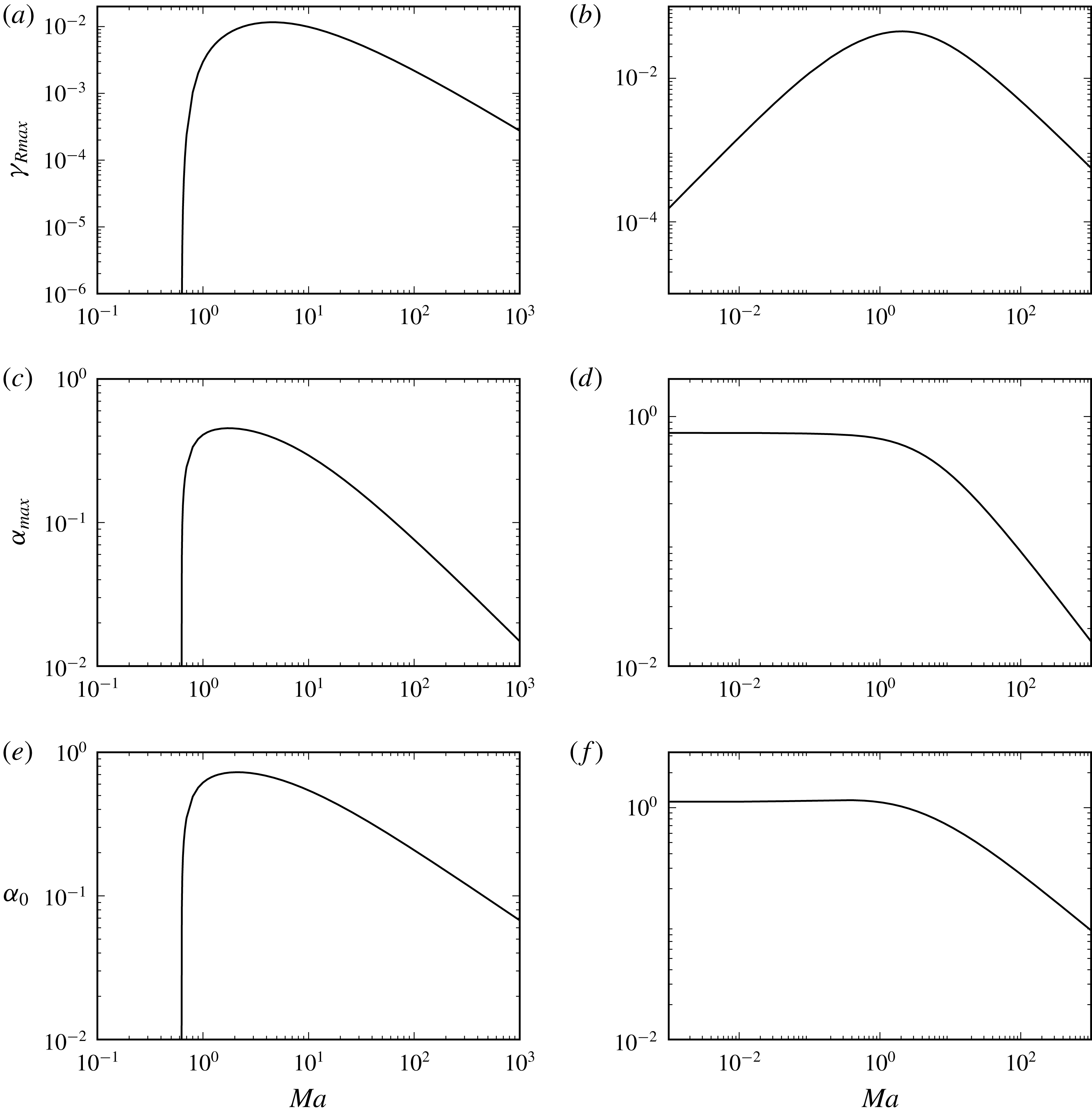
The discontinuity that can occur in the
 $S$
sector is displayed in figure 10. Panel (a) shows that for negligible
 $Bo$
, one branch is long-wave unstable and the other one is stable. As the magnitude of
 $Bo$
increases the previously stable branch becomes unstable (
 $Bo=-1$
) and at some point the branches cross (
 $Bo=-1.5,-2.3$
). Panel (e) shows that as
 $|Bo|$
continues to increase the crossing eventually disappears at which point the upper branch has two local extrema. At some value of
 $Bo$
, the global maximum shifts from the right local extremum (as for
 $Bo=-2.45$
) to the left local extremum (as for
 $Bo=-2.67$
). Finally, as
 $Bo\downarrow -\infty$
, both branches are unstable in the long-wave manner, and feature a single maximum.
5.2 Effects of surfactants in the
$R$
and
$S$
sectors


Here, we investigate, for a fixed value of
 $Bo$
in the
 $R$
and
 $S$
sectors, the Marangoni number
 $Ma$
dependences of the maximum growth rate
 $\unicode[STIX]{x1D6FE}_{max}$
, the corresponding wavenumber
 $\unicode[STIX]{x1D6FC}_{max}$
and the marginal wavenumber
 $\unicode[STIX]{x1D6FC}_{0}$
. The
 $Q$
sector turns out to have somewhat different properties, which are discussed in Part 2. However, it is immediately clear that in the
 $Q$
sector both branches are stable for
 $Bo>0$
and fixed
 $Ma$
(see (c,f,i) in figure 9).
Panels (a,b) of figure 11 show that
 $\unicode[STIX]{x1D6FE}_{Rmax}$
attains a maximum at some
 $Ma=O(1)$
in both the
 $R$
and
 $S$
sectors, and that
 $\unicode[STIX]{x1D6FE}_{Rmax}\downarrow 0$
as
 $Ma\uparrow \infty$
. Both
 $\unicode[STIX]{x1D6FC}_{max}$
and
 $\unicode[STIX]{x1D6FC}_{0}$
also decrease to zero as
 $Ma\uparrow \infty$
. However, in the
 $R$
sector there is a threshold value of
 $Ma$
,
 $Ma_{cL}$
, below which the flow is stable; while in the
 $S$
sector the flow is unstable for all
 $Ma>0$
. Recall from the long-wave results that the linear function
 $Ma_{cL}(Bo)$
is the inverse of
 $Bo_{cL}(Ma)$
(see (4.36) and (4.45)). In the
 $S$
sector,
 $\unicode[STIX]{x1D6FC}_{max}$
and
 $\unicode[STIX]{x1D6FC}_{0}$
approach some non-zero constant values and
 $\unicode[STIX]{x1D6FE}_{Rmax}\downarrow 0$
showing no threshold value of
 $Ma$
for complete stabilization of the flow.
At very small and very large
 $Ma$
, the numerically found behaviour of the marginal wavenumber
 $\unicode[STIX]{x1D6FC}_{0}$
, the maximum growth rate
 $\unicode[STIX]{x1D6FE}_{Rmax}$
and its wavenumber
 $\unicode[STIX]{x1D6FC}_{max}$
(see figure 11) is corroborated with their analytic (or, in some cases, semi-analytic) asymptotic dependencies. The latter are determined as follows.
At
 $Ma\uparrow \infty$
, panels (e,f) suggest that
 $\unicode[STIX]{x1D6FC}_{0}\downarrow 0$
. By substituting (4.13)–(4.15) into the marginal wavenumber equation (3.17), and keeping only the dominant
 $Ma$
terms, the following expression is obtained:
 $$\begin{eqnarray}\displaystyle \frac{n^{2}}{324}(n^{3}+m)^{2}BoMa\unicode[STIX]{x1D6FC}^{2}+\frac{s^{2}}{108}\unicode[STIX]{x1D711}(n-1)(n+1)^{2}(m-n^{2})=0, & & \displaystyle\end{eqnarray}$$
from which
 $$\begin{eqnarray}\displaystyle \unicode[STIX]{x1D6FC}_{0}\approx \frac{s(n+1)\sqrt{3\unicode[STIX]{x1D711}(n-1)(n^{2}-m)}}{n(n^{3}+m)}Bo^{-1/2}Ma^{-1/2}. & & \displaystyle\end{eqnarray}$$
This is consistent with the numerically found behaviour for
 $\unicode[STIX]{x1D6FC}_{0}$
at large
 $Ma$
.
As
 $Ma\downarrow 0$
, it is clear from panel (f) of figure 11 that in the
 $S$
sector,
 $\unicode[STIX]{x1D6FC}_{0}$
approaches some finite non-zero value. Therefore, by keeping only the (dominant) linear
 $Ma$
terms, equation (3.17) reduces to
 $$\begin{eqnarray}\displaystyle k_{11}+k_{13}B^{2}=0. & & \displaystyle\end{eqnarray}$$
However, this equation must be solved numerically for
 $\unicode[STIX]{x1D6FC}_{0}$
since it is not necessarily small. Some other asymptotics for
 $\unicode[STIX]{x1D6FC}_{0}$
approaching zero in the
 $R$
sector were discussed above in § 4.1.2.
At
 $Ma\uparrow \infty$
, panels (a–d) of figure 11 suggest that
 $\unicode[STIX]{x1D6FE}_{Rmax}$
and
 $\unicode[STIX]{x1D6FC}_{max}\downarrow 0$
. By using the long-wave limit and the dominant linear and constant terms of (3.16) for
 $Ma\gg 1$
, we obtain the following asymptotic expressions:
 $$\begin{eqnarray}\displaystyle \unicode[STIX]{x1D6FE}_{Rmax}\approx \frac{ns^{2}(n-1)(n+1)^{2}(m-n^{2})\unicode[STIX]{x1D711}}{4(n^{3}+m)^{3}}Ma^{-1} & & \displaystyle\end{eqnarray}$$
and
 $$\begin{eqnarray}\displaystyle \unicode[STIX]{x1D6FC}_{max}\approx \frac{[12\unicode[STIX]{x1D711}(1-n)(m-n^{2})]^{1/4}(m-1)^{1/2}s}{(n^{3}+m)}Ma^{-3/4}Bo^{-1/4}. & & \displaystyle\end{eqnarray}$$
The details of the derivation are found in Frenkel et al. (Reference Frenkel, Halpern and Schweiger2018).
At
 $Ma\downarrow 0$
, panels (b,d) of figure 11 show that
 $\unicode[STIX]{x1D6FE}_{Rmax}\downarrow 0$
and
 $\unicode[STIX]{x1D6FC}_{max}$
approaches some non-zero constant. Therefore, equation (3.16) is approximately linear for
 $\unicode[STIX]{x1D6FE}_{R}\ll 1$
,
 $$\begin{eqnarray}\displaystyle c_{10}\unicode[STIX]{x1D6FE}_{R}+c_{01}Ma\approx 0 & & \displaystyle\end{eqnarray}$$
so that
 $$\begin{eqnarray}\displaystyle \unicode[STIX]{x1D6FE}_{R}\approx -\frac{c_{01}}{c_{10}}Ma, & & \displaystyle\end{eqnarray}$$
where
 $c_{ij}$
, the coefficients of
 $\unicode[STIX]{x1D6FE}_{R}^{i}Ma^{j}$
in (3.16), are independent of
 $Ma$
. An equation for
 $\unicode[STIX]{x1D6FC}_{max}$
is obtained by differentiating (5.7) with respect to
 $\unicode[STIX]{x1D6FC}$
and solving
 $\text{d}\unicode[STIX]{x1D6FE}_{R}/\text{d}\unicode[STIX]{x1D6FC}=0$
numerically for
 $\unicode[STIX]{x1D6FC}$
, which is then substituted into (5.7) to obtain
 $\unicode[STIX]{x1D6FE}_{Rmax}$
.
Values of (a,b)
 $\unicode[STIX]{x1D6FE}_{Rmax}$
, (c,d)
 $\unicode[STIX]{x1D6FC}_{max}$
and (e,f)
 $\unicode[STIX]{x1D6FC}_{0}$
as functions of
 $Ma$
for
 $Bo=-1.0$
in the
 $R$
sector (a,c,e) and
 $S$
sector (b,d,f), for the same
 $s$
and
 $(n,m)$
points as in figure 11.

In contrast to the case shown in figure 11 for
 $Bo>0$
, the flow is unstable for all
 $Ma$
when
 $Bo<0$
in either the
 $R$
or
 $S$
sectors. Moreover, figure 12(a,b) also shows that
 $\unicode[STIX]{x1D6FE}_{Rmax}$
has a global maximum at
 $Ma=O(1)$
. However, in the
 $S$
sector
 $\unicode[STIX]{x1D6FE}_{Rmax}$
decreases with increasing
 $Ma$
for sufficiently small
 $Ma$
, up to
 $Ma=Ma_{0}$
. At
 $Ma=Ma_{0}$
there is a jump in
 $\unicode[STIX]{x1D6FC}_{max}$
. This behaviour is due to the fact that the dispersion curve has two maxima, and at this particular value of
 $Ma$
there is a jump in the location of the global maximum, similar to that shown in figure 10. Figure 12 also shows that
 $\unicode[STIX]{x1D6FE}_{Rmax}$
,
 $\unicode[STIX]{x1D6FC}_{max}$
and
 $\unicode[STIX]{x1D6FC}_{0}$
all approach some finite positive constant in the limits
 $Ma\uparrow \infty$
and
 $Ma\downarrow 0$
for both sectors. The asymptotics corresponding to figure 12 are obtained below.
Panels (e,f) of figure 12 indicate that
 $\unicode[STIX]{x1D6FC}_{0}$
asymptotes to non-zero constants both at
 $Ma\uparrow \infty$
and at
 $Ma\downarrow 0$
. The relevant values of
 $\unicode[STIX]{x1D6FC}_{0}$
can be obtained as follows.
For
 $Ma\uparrow \infty$
, the dominant term in (3.17) is the
 $Ma^{3}$
term, and since
 $k_{13}\neq 0$
this implies that
 $Bo+\unicode[STIX]{x1D6FC}^{2}\approx 0$
, or
 $$\begin{eqnarray}\displaystyle \unicode[STIX]{x1D6FC}_{0}\approx |Bo|^{1/2}. & & \displaystyle\end{eqnarray}$$
For
 $Bo=-1$
, this yields
 $\unicode[STIX]{x1D6FC}_{0}\approx 1$
which is consistent with the numerical results shown in figure 12(e,f).
In the limit
 $Ma\downarrow 0$
, equation (3.17) reduces to
 $$\begin{eqnarray}\displaystyle (k_{11}+k_{13}B^{2})MaB\approx 0. & & \displaystyle\end{eqnarray}$$
In the
 $R$
sector, the solution
 $\unicode[STIX]{x1D6FC}_{0}\approx |Bo|^{1/2}$
is again obtained because
 $k_{13}$
is always positive and
 $k_{11}$
is the product of
 $(m-1)$
and a positive function, and thus
 $k_{11}>0$
in the
 $R$
sector. However, in the
 $S$
sector
 $k_{11}<0$
, and
 $\unicode[STIX]{x1D6FC}$
is a solution of
 $k_{11}+k_{13}B^{2}=0$
which is solved numerically for
 $\unicode[STIX]{x1D6FC}$
. The solution is approximately
 $\unicode[STIX]{x1D6FC}_{0}\approx 1.56$
, and agrees with figure 12(f).
Finally, consider the asymptotics of
 $\unicode[STIX]{x1D6FE}_{Rmax}$
and
 $\unicode[STIX]{x1D6FC}_{max}$
in the limit
 $Ma\uparrow \infty$
, and then in the limit
 $Ma\downarrow 0$
, (panels (a–d) of figure 12). At
 $Ma\uparrow \infty$
, the terms proportional to
 $Ma^{3}$
in (3.16) yield a linear equation for
 $\unicode[STIX]{x1D6FE}_{R}$
. Hence,
 $$\begin{eqnarray}\displaystyle \unicode[STIX]{x1D6FE}_{R}\approx -\frac{1}{2}\frac{(s_{\unicode[STIX]{x1D6FC}}^{2}-\unicode[STIX]{x1D6FC}^{2})(s_{\unicode[STIX]{x1D6FC}n}^{2}-\unicode[STIX]{x1D6FC}^{2}n^{2})(Bo+\unicode[STIX]{x1D6FC}^{2})}{\unicode[STIX]{x1D6FC}(s_{\unicode[STIX]{x1D6FC}}^{2}-\unicode[STIX]{x1D6FC}^{2})(s_{\unicode[STIX]{x1D6FC}n}c_{\unicode[STIX]{x1D6FC}n}+\unicode[STIX]{x1D6FC}n)m+\unicode[STIX]{x1D6FC}(s_{\unicode[STIX]{x1D6FC}n}^{2}-\unicode[STIX]{x1D6FC}^{2}n^{2})(s_{\unicode[STIX]{x1D6FC}}c_{\unicode[STIX]{x1D6FC}}+\unicode[STIX]{x1D6FC})}. & & \displaystyle\end{eqnarray}$$
Again, one must solve
 $\text{d}\unicode[STIX]{x1D6FE}_{R}/\text{d}\unicode[STIX]{x1D6FC}=0$
numerically for
 $\unicode[STIX]{x1D6FC}_{max}$
which in turn is substituted into (5.10) to obtain
 $\unicode[STIX]{x1D6FE}_{Rmax}$
. At
 $Ma\downarrow 0$
, the terms without
 $\unicode[STIX]{x1D6FE}_{R}$
in (3.16) vanish, and the asymptotic constant values are found, similarly, from
 $\unicode[STIX]{x1D6FE}_{R}=-c_{10}/c_{20}$
.
Figure 13 shows the results of varying the shear parameter
 $s$
. For any fixed
 $s$
, the growth rate has a global maximum over the
 $(\unicode[STIX]{x1D6FC},Ma)$
-plane, denoted
 $\text{max}\unicode[STIX]{x1D6FE}_{R}$
. We denote
 $\unicode[STIX]{x1D6FC}(\text{max}\unicode[STIX]{x1D6FE}_{R})$
and
 $Ma(\text{max}\unicode[STIX]{x1D6FE}_{R})$
the values of the wavenumber and Marangoni number, respectively, at which the growth rate attains its maximum,
 $\text{max}\unicode[STIX]{x1D6FE}_{R}$
. These quantities are plotted versus
 $s$
in figure 13, for selected sampling points in the
 $R$
and
 $S$
sectors. We see that while in (a,c) the dependencies are linear, and also practically independent of the Bond number, this does not hold for the
 $\unicode[STIX]{x1D6FC}(\text{max}\unicode[STIX]{x1D6FE}_{R})$
shown in panel (b); in particular, in all four cases shown there, it stays almost constant (of magnitude order 1) at large
 $s$
but falls off precipitously to zero as
 $s$
approaches zero.
In this subsection we only had to deal with the long-wave instability because the values of
 $Ma$
considered are either sufficiently large or sufficiently small, or the viscosity ratio was not sufficiently close to the
 $R-Q$
boundary
 $m=n^{2}$
. It turns out that for the intermediate values of
 $Ma$
and the appropriate values of
 $m$
, even in the
 $R$
sector, a different type of instability, called the ‘mid-wave’ instability (Halpern & Frenkel Reference Halpern and Frenkel2003), may happen. It is considered in Part 2.
The influence of
 $s$
on (a) the maximum of
 $\unicode[STIX]{x1D6FE}_{Rmax}$
over all
 $\unicode[STIX]{x1D6FC}$
and
 $Ma$
in the
 $R$
sector (at
 $n=2$
and
 $m=2$
) and the
 $S$
sector (at
 $n=2,m=0.5$
) for two different values of
 $Bo$
as indicated in the legend. Panels (b,c) show the corresponding
 $\unicode[STIX]{x1D6FC}$
and
 $Ma$
.

6 Summary and discussion
In this paper, we have considered the linear stability of two immiscible viscous fluid layers flowing in the channel between two parallel plates that may move steadily with respect to each other driving a Couette flow. The combined effects of gravity and an insoluble surfactant monolayer at the fluid interface were examined for certain flows such that the effect of inertia on their stability properties is negligible. The bulk velocity components satisfy linear homogeneous equations with constant coefficients. Therefore, their general solution, in the standard normal-mode analysis, is available with a few undetermined constants. The latter are determined, by the plate and interfacial-balance boundary conditions, in terms of the interface deflection and surfactant disturbance amplitudes. This yields a system of two algebraic linear homogeneous equations for the latter two amplitudes. Non-trivial solutions of this algebraic eigenvalue problem exist only if the increment
 $\unicode[STIX]{x1D6FE}$
, the complex ‘growth rate’, satisfies a quadratic equation whose coefficients are known functions of the wavenumber
 $\unicode[STIX]{x1D6FC}$
, the Marangoni number
 $Ma$
, the Bond number
 $Bo$
, the viscosity ratio
 $m$
, the aspect ratio
 $n$
and the interfacial shear parameter
 $s$
. The two solutions of this dispersion equation were shown to yield two continuous increment branches, defined almost everywhere in the (wavenumber, system parameters)-space (with a ‘branch cut’ hypersurface excluded from it), and their real parts, the two continuous growth rate branches, were analysed to infer conclusions concerning the stability of the flow. Similar to FH and subsequent papers, we call one of the branches the ‘robust’ branch, as it is present even when
 $Ma=0$
, and we call the other one, that vanishes as
 $Ma\downarrow 0$
, the ‘surfactant’ branch. Thus, we have explicit formulas allowing us to readily compute the growth rates of instability for any given input values of the wavenumber and the five parameters of the problem.
In the long-wave analysis of FH, three open sectors in the part of the (
 $n$
,
 $m$
)-plane given by
 $n\geqslant 1$
and
 $m\geqslant 0$
, categorizing the stability of the system without gravity (
 $Bo=0$
), were identified: the
 $Q$
sector, (
 $m>n^{2}$
), where both modes are stable; the
 $R$
sector, (
 $n^{2}>m>1$
), where only the robust branch is unstable; and the
 $S$
sector, (
 $0<m<1$
), where only the surfactant mode is unstable. The same long-wave sectors were found to be relevant for non-zero
 $Bo$
in the lubrication theory of Frenkel & Halpern (Reference Frenkel and Halpern2017). In the present paper, by using the long-wave asymptotics for the coefficients of the quadratic dispersion equation, we corroborate the lubrication approximation results of Frenkel & Halpern (Reference Frenkel and Halpern2017) for the instability thresholds. In the
 $S$
sector, the surfactant mode remains unstable for all
 $Bo$
, that is for arbitrarily strong stabilizing gravity; while in the
 $R$
sector the growth rate of the robust branch is unstable provided
 $Bo$
is below some positive threshold value
 $Bo_{c}$
. In the
 $Q$
sector, both branches remain stable for
 $Bo\geqslant 0$
, but the robust branch is long-wave unstable for the smaller values of
 $Ma$
(while mid-wave unstable for larger values of
 $Ma$
, so that there are longer waves that are stable, as discussed below), when
 $Bo$
is below some negative
 $Bo_{c}$
. We have obtained the long-wave marginal wavenumbers and extremum growth rates which depend on the two main orders of the growth rate expression and were not considered in Frenkel & Halpern (Reference Frenkel and Halpern2017). In particular, the small-
 $s$
behaviour of the marginal wavenumber was obtained from the asymptotic form of our general equation for the marginal wavenumber. We have established that in the
 $R$
sector there are parametric situations in which the stabilizing effects, responsible for the emergence of the marginal wavenumber, are due, instead of the capillary forces, as is usual for larger
 $s$
, to the non-trivial combined action of gravitational and surfactant forces.
We also obtained the asymptotic small-
 $s$
behaviour of the (long-wave) growth-rate maximum and its corresponding wavenumber, which yielded different power laws for the cases of zero and non-zero Bond numbers. The asymptotic behaviour in nearing the instability thresholds in the different sectors was established as well.
The long-wave instabilities at the different borders between the three (
 $n,m$
)-sectors were analysed, such as the
 $S-R$
one,
 $m=1$
. For the latter case, it was not clear from the small-wavenumber expression for the growth rates, equation (4.49), whether the unstable mode belonged to the surfactant branch, or, alternatively, to the robust one. We used complex analysis to show that there are indeed two separate branches of the growth-rate function continuous for all wavenumbers and all the values of the parameters, one of the branches everywhere positive and the other one everywhere negative. The surfactant branch is easily identified near the wavenumber axis in the (wavenumber, Marangoni number)-space, as the one of the two branches which vanishes in the limit of Marangoni number approaching zero, and it turns out to be positive or negative for positive or negative Bond number, respectively. The same is then true in the alternative limit, the wavenumber approaching zero at a finite Marangoni number, (corresponding to (4.49)), since the branches keep their signs everywhere, and in particular the surfactant branch of the growth rate has the same sign near the
 $Ma$
-axis as its sign near the
 $\unicode[STIX]{x1D6FC}$
-axis. In this way, we established that the unstable mode, corresponding to the positive sign in (4.49), belongs to the surfactant (robust) branch for positive (negative) Bond numbers (and the stable mode belongs to the other branch, in each case).
For cases of arbitrary, (not necessarily small) wavenumbers, we still have explicit formulas for the stability quantities of interest, albeit more complicated and therefore, in general, studied numerically. It was found that in the
 $S$
sector and in the
 $R$
sector sufficiently far from the
 $Q$
sector, as well as in the
 $Q$
sector for sufficiently small Marangoni numbers, the dominant-mode instability has a long-wave character, in the sense that the left endpoint of the interval of unstable wavenumbers is zero. Otherwise, in particular in the
 $Q$
sector, for sufficiently large Marangoni numbers, the ‘mid-wave’ instability may occur, in which the interval of unstable wavenumbers is bounded away from zero. An interesting phenomenon, the dispersion-curve reconnection, was observed in the
 $S$
sector. Both branches are unstable for sufficiently negative values of Bond number, and, as
 $Bo$
decreases further, the robust-mode dispersion curve starts to cross the other dispersion curve at a single intersection point. Later in this process, at some sufficiently large value of
 $|Bo|$
, the four parts of the two curves emanating from the intersection point recombine and detach, forming two new, non-intersecting, continuous curves, with the upper curve having two local maxima, of unequal heights. Then, as the Bond number decreases further, a jump in the global maximum may occur, as the shorter local maximum grows and eventually overcomes the other local maximum (figure 10).
The long-wave instability was studied with respect to gravity effects, as indicated by the dependencies of the characteristic dispersion quantities on the Bond number, figure 9, and, in the
 $S$
and
 $R$
sectors, with respect to the surfactant effects, as expressed in the dependencies on the Marangoni number, figures 11 and 12. For the small and large values of these parameters, the relevant wavenumbers may be small, allowing for simpler asymptotics. Even when the limits of the characteristic dispersion quantities are not small, we sometimes get simplified equations which are easier to solve numerically, or, occasionally, even approximate analytic expressions, such as (5.8).
In the
 $R$
and
 $S$
sectors, at a fixed Bond number, the long-wave growth rate has a maximum at certain finite values of the wavenumber and the Marangoni number. We have observed, numerically, that both the maximum growth rate and its Marangoni number, grow linearly with the shear parameter
 $s$
, starting from zero, while the corresponding wavenumber, which starts from zero as well, grows very fast at first, but then remains almost constant at larger
 $s$
(figure 13).
Appendix A. On the continuous branches of the growth-rate function
Recall that the two distinct analytic branches of the function
 $\sqrt{\unicode[STIX]{x1D701}}$
exist in any simply connected domain in the complex plane that does not contain the origin (
 $\unicode[STIX]{x1D701}=0$
). As was mentioned in the text, it may happen for the discriminant
 $\unicode[STIX]{x1D701}$
of the dispersion relation that
 $\unicode[STIX]{x1D701}=0$
for some values of
 $\unicode[STIX]{x1D6FC}$
and the parameters. This implies the two real equations,
 $\text{Re}(\unicode[STIX]{x1D701})=0$
and
 $\text{Im}(\unicode[STIX]{x1D701})=0$
. The imaginary part of
 $\unicode[STIX]{x1D701}$
(3.15) is
 $$\begin{eqnarray}\displaystyle \text{Im}(\unicode[STIX]{x1D701})=\frac{s}{\unicode[STIX]{x1D6FC}^{5}}\left(k_{Ma}Ma+\frac{k_{b}}{\unicode[STIX]{x1D6FC}^{2}}(Bo+\unicode[STIX]{x1D6FC}^{2})\right). & & \displaystyle\end{eqnarray}$$
Here,
 $k_{M\unicode[STIX]{x1D6FC}}$
and
 $k_{b}$
are known functions of
 $m$
,
 $n$
and
 $\unicode[STIX]{x1D6FC}$
, given explicitly in appendix A of Frenkel et al. (Reference Frenkel, Halpern and Schweiger2018). As we mentioned before, the two equations
 $\text{Re}(\unicode[STIX]{x1D701})=0$
and
 $\text{Im}(\unicode[STIX]{x1D701})=0$
define a manifold of codimension two in the
 $\unicode[STIX]{x1D6FC}$
-parameter space. This manifold is analogous to a multivalued-function branch point in the complex plane. We consider the trace of this ‘branch manifold’ in the three-dimensional space of
 $(\unicode[STIX]{x1D6FC},Ma,Bo)$
, with the rest of the parameters fixed, as follows. Solving
 $\text{Im}(\unicode[STIX]{x1D701})=0$
for Marangoni number yields
 $$\begin{eqnarray}\displaystyle Ma=-\frac{k_{b}}{\unicode[STIX]{x1D6FC}^{2}k_{Ma}}(Bo+\unicode[STIX]{x1D6FC}^{2}). & & \displaystyle\end{eqnarray}$$
Note that not all values of (
 $Bo,Ma$
) are appropriate here because
 $Ma$
must be positive.
Similarly to the above expression for
 $\text{Im}(\unicode[STIX]{x1D701})$
, we obtain
 $$\begin{eqnarray}\displaystyle Re(\unicode[STIX]{x1D701})=\frac{1}{\unicode[STIX]{x1D6FC}^{10}}(K_{20}Ma^{2}+K_{02}(Bo+\unicode[STIX]{x1D6FC}^{2})^{2}+K_{11}Ma(Bo+\unicode[STIX]{x1D6FC}^{2})+K_{00}), & & \displaystyle\end{eqnarray}$$
Here,
 $K_{ij}$
are functions of
 $m$
,
 $n$
and
 $\unicode[STIX]{x1D6FC}$
(for their explicit forms, see appendix A of Frenkel et al. (Reference Frenkel, Halpern and Schweiger2018)). To solve the system
 $\text{Re}(\unicode[STIX]{x1D701})=0$
and
 $\text{Im}(\unicode[STIX]{x1D701})=0$
for
 $Ma$
and
 $Bo$
as functions of
 $\unicode[STIX]{x1D6FC}$
(with
 $s$
,
 $m$
, and
 $n$
fixed), equation (A 2) is substituted into
 $\text{Re}(\unicode[STIX]{x1D701})$
which yields
 $$\begin{eqnarray}\displaystyle \text{Re}(\unicode[STIX]{x1D701})=AB^{2}+C=0, & & \displaystyle\end{eqnarray}$$
where
 $B=Bo+\unicode[STIX]{x1D6FC}^{2}$
, and
 $A$
and
 $C$
do not depend on
 $Ma$
:
 $$\begin{eqnarray}\displaystyle A=\frac{1}{\unicode[STIX]{x1D6FC}^{10}}\left(\frac{k_{b}^{2}}{\unicode[STIX]{x1D6FC}^{4}k_{Ma}^{2}}K_{20}+K_{02}-\frac{k_{b}}{\unicode[STIX]{x1D6FC}^{2}k_{Ma}}K_{11}\right),\quad C=\frac{K_{00}}{\unicode[STIX]{x1D6FC}^{10}}. & & \displaystyle\end{eqnarray}$$
Therefore,
 $Bo=Bo(\unicode[STIX]{x1D6FC})$
, (without explicitly indicating the additional dependence on
 $m$
,
 $n$
and
 $s$
), where
 $$\begin{eqnarray}\displaystyle Bo(\unicode[STIX]{x1D6FC})=-\unicode[STIX]{x1D6FC}^{2}\pm \sqrt{-\frac{C}{A}}. & & \displaystyle\end{eqnarray}$$
Substituting (A 6) for
 $Bo$
into (A 2) yields
 $Ma$
such that
 $\unicode[STIX]{x1D701}=0$
for a given
 $\unicode[STIX]{x1D6FC}$
. Only the unique value
 $Bo=Bo(\unicode[STIX]{x1D6FC})$
that yields
 $Ma=Ma(\unicode[STIX]{x1D6FC})>0$
is admitted here. In figure 14(a,b) curves
 $Bo=Bo(\unicode[STIX]{x1D6FC})$
and
 $Ma=Ma(\unicode[STIX]{x1D6FC})$
are plotted for various values of
 $m$
with
 $n$
fixed at 2 and
 $s$
fixed at 1. One can see that
 $Ma\uparrow \infty$
in the limit
 $\unicode[STIX]{x1D6FC}\downarrow 0$
for all
 $m$
. In this limit,
 $Bo\uparrow \infty$
for
 $m>1$
, but
 $Bo\uparrow -\infty$
for
 $m<1$
. At
 $\unicode[STIX]{x1D6FC}\uparrow \infty$
, for all
 $m$
,
 $Bo\sim -\unicode[STIX]{x1D6FC}^{2}$
and
 $Ma\downarrow 0$
. There are no points where the discriminant is zero for
 $m=1$
, as was shown in the main text for all parameter values (formally, in the figure, we get
 $Ma(\unicode[STIX]{x1D6FC})=0$
and
 $Bo(\unicode[STIX]{x1D6FC})=-\unicode[STIX]{x1D6FC}^{2}$
). This indicates that the branch manifold consists of at least two pieces, and perhaps more than two, some with
 $m>1$
and others with
 $m<1$
. The same fact is reflected in the infinite discontinuities of the curves in the figure at finite values of
 $\unicode[STIX]{x1D6FC}$
, which take place provided
 $m>n^{2}$
.
The curves (a)
 $Bo=Bo(\unicode[STIX]{x1D6FC})$
and (b)
 $Ma=Ma(\unicode[STIX]{x1D6FC})$
such that the discriminant
 $\unicode[STIX]{x1D701}=0$
are plotted for the values of viscosity ratio
 $m$
indicated in the legend. Here
 $n=2$
and
 $s=1$
.

The zero discriminant curve corresponding to the
 $m=2$
projection curves shown in (a,b) of figure 14.

Also, if we consider the (
 $\unicode[STIX]{x1D6FC}$
,
 $Ma$
)-plane, with all the other parameters fixed, including
 $Bo$
, corresponding to a horizontal line in figure 14(a), there will be at most two branch points in the (
 $\unicode[STIX]{x1D6FC},Ma$
)-plane since any horizontal line there intersects any curve at no more than two points. Therefore, in some sufficiently narrow infinite strip whose left boundary is the (vertical)
 $Ma$
-axis, the discriminant is non-zero at all its points, and so there are two continuous branches, in agreement with the long-wave results in the main text. These results also show no intersections of the two dispersion curves (when the wavenumbers are small enough), which means that
 $\text{Re}\sqrt{\unicode[STIX]{x1D701}}$
is non-zero in a sufficiently narrow strip bordering the
 $Ma$
-axis. The equation
 $\text{Re}\sqrt{\unicode[STIX]{x1D701}}=0$
implies that
 $\unicode[STIX]{x1D701}$
is real (and negative). We have solved this equation for
 $Ma$
as a function of
 $\unicode[STIX]{x1D6FC}$
at fixed values of
 $Bo$
(and the other parameters), and every resulting curve in the (
 $\unicode[STIX]{x1D6FC},Ma$
)-plane indeed lies entirely outside some strip bordering the
 $Ma$
-axis.
Regarding the entire (
 $\unicode[STIX]{x1D6FC},Ma$
)-plane, if we remove from it the branch points together with the infinite rays emanating from each branch point to the right and going parallel to the
 $\unicode[STIX]{x1D6FC}$
-axis (the branch cuts), then in the remaining domain the discriminant is nowhere zero, and thus there are two continuous branches of the growth rate in this domain, smooth in
 $\unicode[STIX]{x1D6FC}$
at each point that they are defined.
Note that the horizontal line
 $Bo=0$
in (a) of figure 14 intersects every curve whose
 $m>1$
. So, even in the absence of gravity, there may be intersections of the two dispersion curves. As
 $Ma$
is varied, these intersections disappear at some
 $Ma$
, with the reconnection of the curve parts lying to the right of the ‘marginal intersection’ point and consequent separation of the two ‘renovated’ dispersion curves. This happens in the ranges of wavenumbers when both branches are stable, which was not noted in HF.
Figure 15 shows, as an example, the curve in the three-dimensional space which corresponds to the two dash-dotted,
 $m=2$
, curves of figure 14. The coordinate box there is shown with its front, top and right faces removed for a better view. The curve of zero discriminant starts at the back top right vertex and steadily goes downward and to the left simultaneously twisting first toward the viewer and then backward, until it ends at the back bottom left vertex.
We note that there is always a strip
 ${\mathcal{D}}_{s}=\{0<\unicode[STIX]{x1D6FC}<\unicode[STIX]{x1D6FC}_{s},Ma>0\}$
where
 $\unicode[STIX]{x1D701}\neq 0$
. Indeed, it appears in figure 14(a) that any horizontal line
 $Bo=Bo_{f}$
intersects any of the graphs of
 $Bo=Bo_{m}(\unicode[STIX]{x1D6FC})$
at no more than three points. If there are no intersections then the value of
 $\unicode[STIX]{x1D6FC}_{s}$
is chosen completely arbitrarily. Otherwise,
 $\unicode[STIX]{x1D6FC}_{s}$
must be smaller than the smallest
 $\unicode[STIX]{x1D6FC}$
of the intersection points. For the purpose of this paper, the existence of
 ${\mathcal{D}}_{s}$
(and thus of the two branches of the growth rate) is sufficient with any small but finite
 $\unicode[STIX]{x1D6FC}_{s}$
. The existence of
 $\unicode[STIX]{x1D6FC}_{s}$
is confirmed analytically for the small values of
 $\unicode[STIX]{x1D6FC}$
.