2.1. Numerical method

In this study, the governing equations used for simulating PS and VD SBI are the compressible Navier–Stokes equations with multiple components, expressed as

(2.1) \begin{equation} \left \{ \begin{aligned} & \frac{\partial {\rho }}{\partial t} + \frac{\partial ({\rho }{u_i})}{\partial {x_i}} = 0, \\ & \frac{\partial \left ({\rho }{u_i}\right )}{\partial t} + \frac{\partial ({\rho }{u_i}{u_{\!j}})}{\partial {x_{\!j}}} = -\frac{\partial {p}}{\partial {x_i}} + \frac{\partial {\sigma }_{\textit{ij}}}{\partial {x_{\!j}}}, \\ & \frac{\partial ({\rho }{E})}{\partial {t}} + \frac{\partial ({\rho }{u_i}{H})}{\partial {x_i}} = -\frac{\partial {q_i}}{\partial {x_i}} + \frac{\partial ({u_{\!j}}{\sigma }_{\textit{ij}})}{\partial {x_i}},\\ &\frac{\partial ({\rho }{Y}_m)}{\partial {t}} + \frac{\partial ({\rho }{u_i}{Y}_m)}{\partial {x_i}} = \frac{\partial }{\partial {x_i}}\left ({\rho }\mathcal{D}\frac{\partial {Y}_m}{\partial {x_i}}\right )\!,\\ & m = 1,2,{\cdots} ,s-1. \end{aligned} \right . \end{equation}

Here, the symbols $\rho$ , $p$ , $E$ and $H = E + {p}/{\rho }$ denote the mixture’s density, pressure, total energy per unit mass and total enthalpy per unit mass, respectively, $u_i$ is the velocity of the mixture in the $i$ th direction, $Y_{m}$ refers to the mass fraction of species $m$ with $\sum \limits _{m=1}^{s} Y_{m} = 1$ and $s$ is labelled as the total number of species. With the ideal gas hypothesis and Dalton’s law of partial pressures, the system of (2.1) is closed by the ideal gas state equation

(2.2) \begin{equation} p = \sum \limits _{m=1}^{s} p_{m} = \sum \limits _{m=1}^{s} \rho _{m}\frac{\mathcal{R}_{0}}{M_{m}}T = \rho \mathcal{R}T = \left (\gamma - 1\right )\rho e, \end{equation}

where $\mathcal{R} = \mathcal{R}_{0}/M$ and $\mathcal{R}_{0} = 8.314\ \rm {J (mol\ K)^{-1}}$ are the gas constant and universal gas constant, respectively; 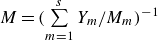$M = (\sum \limits _{m=1}^{s}Y_{m}/M_{m})^{-1}$ and $T$ are the molar mass and temperature of mixture respectively; $p_{m}, \rho _{m} = \rho Y_{m}$ and $M_{m}$ represent the partial pressure, density and molar mass of the component $m$ , respectively. The relation of the total energy per unit mass $E$ and the specific internal energy $e$ is given by

(2.3) \begin{equation} E = e + \frac{1}{2} u_{i}u_{i} = h - \frac{p}{\rho } + \frac{1}{2} u_{i}u_{i}. \end{equation}

Here, $h$ is the enthalpy of the gas mixture

(2.4) \begin{equation} h = \sum \limits _{m=1}^{s} Y_{m}h_{m} = \sum \limits _{m=1}^{s} Y_{m}\left (h_{fm}^{0} + \int _{T_0}^{T}\frac{C_{pm}}{M_{m}}dT\right )\!, \end{equation}

in which $h_{fm}^{0}$ is the heat generated by the component $m$ at the reference temperature $T_{0}$ . The constant-pressure specific heat value $C_{pm}$ is fitted by the following temperature-dependent polynomial function:

(2.5) \begin{equation} C_{pm} = \mathcal{R}_{0}(a_{1m} + a_{2m}T + a_{3m}T^2 + a_{4m}T^3 + a_{5m}T^4), \end{equation}

where the coefficients $a_{1m},\ldots .,a_{5m}$ are obtained from the NASA thermochemical polynomial fit coefficient data (Kee et al. Reference Kee, Rupley, Meeks and Miller1996).

With the definition of the constant-volume specific heat

(2.6) \begin{equation} C_{pm} - C_{vm} = \frac{\mathcal{{R}}_{0}}{M_{m}}, \end{equation}

the constant-pressure specific heat and constant-volume specific heat of the gas mixture are $C_p = \sum \limits _{m=1}^{s} Y_{m}C_{pm}$ and $C_v = \sum \limits _{m=1}^{s} Y_{m}C_{vm}$ , and the specific heat ratio of the gas mixture is $\gamma = C_{p}/C_{v}$ .

For the Newtonian fluid considered in this work, the viscous stress tensor and heat flux are defined as

(2.7) \begin{equation} \left \{ \begin{aligned} & {\sigma }_{\textit{ij}} = \mu \left (\frac{\partial {u_i}}{\partial {x_{\!j}}} + \frac{\partial {u_{\!j}}}{\partial {x_i}} - \frac{2}{3}\delta _{\textit{ij}}\frac{\partial {u_k}}{\partial {x_k}}\right )\!, \\ & {q_i} = -\lambda \frac{\partial {T}}{\partial {x_i}}.\end{aligned} \right . \end{equation}

Here, $\delta _{\textit{ij}}$ refers to the Kronecker delta. Based on the observation that the transport coefficients converge to nearly steady values after shock interaction (Liu et al. Reference Liu, Yu, Zhang and Xiang2022), constant transport coefficients are employed in the numerical simulations to simplify the expression of the mixing model in the subsequent sections. Specifically, the viscous stress tensor ${\sigma }_{\textit{ij}}$ is calculated by the constant dynamic viscosity $\mu = 125 \times 10^{-6}\, \rm {Pa\boldsymbol{\cdot }s}$ . The mass diffusion is simplified by ignoring pressure and temperature diffusion, and the Fickian diffusivity is assumed to be constant for different components, with a value of $\mathcal{D} = 355 \times 10^{-6}\, {\textrm {m}^2\,\rm s^{-1}}$ . Setting the diffusivity $\mathcal{D}$ as a constant does not accurately reflect the true physical situation. Assigning a constant value to $\mathcal{D}$ is typically used when designing SBI cases with varying Péclet numbers, which has also been employed in our previous studies (Yu et al. Reference Yu, Liu and Liu2021, Reference Yu, Li, Xu, Zhang and Liu2022). The heat flux $q_{i}$ is calculated by the Fourier’s law of heat conduction, and the heat conduction coefficient $\lambda = C_p \mu /Pr$ is calculated using a constant Prandtl number $Pr = 0.72$ . After the mathematical model is constructed, the compressible Navier–Stokes equations are numerically solved using an in-house high-resolution code, ${\textit{ParNS3D}}$ , which has undergone extensive validation (Wang et al. Reference Wang, Yu, Chen, Zhang and Liu2018; Liang et al. Reference Liang, Yu, Zhang, Xu and Liu2019; Yu et al. Reference Yu, Li, Xu, Zhang and Liu2022; Liu et al. Reference Liu, Yu, Zhang and Xiang2022). Temporal discretisation is performed using the third-order total variation diminishing Runge–Kutta method. The fifth-order weighted essentially non-oscillatory (WENO) scheme (Liu et al. Reference Liu, Osher and Chan1994; Jiang & Shu Reference Jiang and Shu1996) is employed for the discretisation of convection terms, while the second-order central difference method discretises the viscous terms.

2.2. Initial conditions for VD and PS SBI

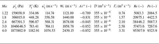
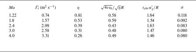
This section presents the initial conditions for the numerical simulation of VD and PS SBI, using a case with a shock strength of ${\textit{Ma}} = 2.4$ as an example. The case settings for other simulations, covering a broad range of Mach numbers from $1.22$ to $4$ , are provided in Appendix A. The configuration for VD SBI settings is depicted in figure 1 $(a)$ . The computation domain encompasses a two-dimensional space in a Cartesian coordinate system, with $X \times Y = [0, L_x] \times [0, L_y]$ , where the length is $L_x = 30 \,\rm {mm}$ and the height is $L_y = 5.5\,\rm {mm}$ . The shock is positioned at $x_{shock} = 0.7\,\rm {mm}$ . The pre-shock air has the same thermodynamic states of $1\,\rm {atm}$ pressure and $293\,\rm {K}$ temperature prior to being impacted by the shock. The detailed initial conditions for post-shock air ( $u_{1}^{\prime}, \rho _{1}^{\prime}, P_{1}^{\prime}$ and $T_{1}^{\prime}$ ) are calculated from the Rankine–Hugoniot equation. To avoid spurious vorticity arisen from the mesh discretisation (Niederhaus et al. Reference Niederhaus, Greenough, Oakley, Ranjan, Anderson and Bonazza2008), the helium bubble, centred at the position $x_{bubble} = 4.5\,\rm {mm}$ , consists of a core region with a radius of $R=2.5\,{\textrm {mm}}$ and a diffusive layer with a width of $\delta$ . The diffusive layer is positioned at the edge of the core region, as illustrated in the inset in figure 1 $(a)$ . Based on this configuration, the distribution of mass fraction of helium is set as

(2.8) \begin{equation} Y_{\textit{He}}(r) = \left \{ \begin{aligned} & Y_{\textit{max}}, & &r \lt R, \\ & Y_{\textit{max}}\mathrm{e}^{-\alpha [(r-R)/\delta ]^2}, & & R \leqslant r \lt R + \delta , \\ & 0, & &r \geqslant R + \delta , \end{aligned} \right . \end{equation}

where $Y_{\textit{max}} = 1.0$ , $\alpha = 5$ and $\delta =5$ . Using these parameters, the mass fraction distribution across the bubble is shown in figure 1 $(b)$ . It can be observed that, with the selected parameters in (2.8), the mass fraction within the thin diffusive layer smoothly connects the mass fraction inside and outside the bubble, which is consistent with the results reported in our previous studies (Wang et al. Reference Wang, Yu, Chen, Zhang and Liu2018; Liu et al. Reference Liu, Yu, Zhang and Xiang2022; Yu et al. Reference Yu, Li, Xu, Zhang and Liu2022). To simplify subsequent expressions, the helium mass fraction $Y_{\textit{He}}$ is denoted as $Y$ .

Figure 1.

$(a)$ Schematic of the initial conditions for VD SBI. $(b)$ Distribution of the initial mass fraction of helium $Y_{\textit{He}}$ across the diameter of the bubble.

Since the influence of the reflected pressure wave on mixing is not considered in this study, the left boundary is set as an inlet, while the upper and right boundaries utilise a fourth-order extrapolation to prevent interference from pseudo-pressure reflection waves affecting the flow structures of interest. A symmetric boundary condition is applied at the bottom of the computational domain. The grid resolution study, detailed in Appendix B, demonstrates that a uniform grid with a spacing of ${\varDelta } = 1.25 \times 10^{-5}\,\rm {m}$ is sufficient to accurately resolve the mixing process for the VD SBI case. Accordingly, the time step for the numerical simulation is selected as $\Delta t = 2\times 10^{-9}\ {\textrm {s}}$ to ensure the Courant-Friedrichs-Lewy number satisfies the condition

(2.9) \begin{equation} {\textrm {CFL}} = \frac{\Delta t}{\varDelta /u_{\textit{max}}} \approx \frac{\Delta t}{\varDelta /u_2^{\prime}} \lt 1. \end{equation}

Here, $u_2^{\prime}$ indicates the post-shock velocity of the helium bubble, which approximates the maximum velocity within the computation domain.

To investigate the stretching dynamics and its impact on mixing in VD SBI, we begin by developing a quantitative mixing model using a relatively simple PS SBI case. In this scenario, the density difference between the post-shock bubble and the ambient air is eliminated, specifically, by setting the post-shock Atwood number $At^{+} = (\rho _2^{\prime} - \rho _1^{\prime})/(\rho _2^{\prime} + \rho _1^{\prime}) \approx 0$ , where $\rho _2^{\prime}$ and $\rho _1^{\prime}$ represent the post-shock bubble density and ambient air density, respectively. This adjustment allows the density effects to be effectively neglected as the vortex develops, ensuring that the mixing process does not influence the flow dynamics, as expected in PS mixing (Dimotakis Reference Dimotakis2005). However, the formation of the primary vortex depends on the baroclinic vorticity generated by the cylindrical interface of fluids with different densities subjected to a shock. If the density of the original bubble matches that of the ambient air, no vorticity is deposited along the bubble interface. Therefore, an artificial density adjustment method is applied to complete the set-up of the initial conditions for the PS SBI. On the basis of the VD SBI case with the shock Mach number ${\textit{Ma}}=2.4$ , the cylindrical bubble’s mass fraction is adjusted artificially soon after the shock interaction

(2.10) \begin{equation} \left \{ \begin{aligned} & Y_{\textit{He}}^{\textit{ps}}=0.0001\times Y_{\textit{He}}^{\textit{VD}},\\ & Y_{O_2}^{\textit{ps}}=0.233\times \left (1 - Y_{\textit{He}}^{\textit{ps}}\right )\!,\\ & Y_{N_2}^{\textit{ps}}=0.767\times \left (1 - Y_{\textit{He}}^{\textit{ps}}\right )\!, \end{aligned} \right . \end{equation}

where a small amount of component is maintained to display the mixing process. With the pressure and temperature identical to those in VD SBI

(2.11) \begin{equation} \left \{ \begin{aligned} & p^{\textit{ps}}=p^{\textit{VD}},\\ & T^{\textit{ps}}=T^{\textit{ps}}, \end{aligned} \right . \end{equation}

the density of the bubble after the shock interaction will increase to the value of post-shock air

(2.12) \begin{equation} \left \{ \begin{aligned} & \rho ^{\textit{ps}}=\frac{p^{\textit{ps}}}{\mathcal{R}T^{\textit{ps}}}\approx \rho ^{\textit{air}},\\ & \mathcal{R}=\mathcal{R}_{0}\sum _{m=1}^{s}\frac{Y_{m}^{\textit{ps}}}{M_{m}}. \end{aligned} \right . \end{equation}

To ensure comparability of the mixing indicators between PS SBI and VD SBI, the mass fraction in PS SBI, denoted $Y^{\textit{ps}}$ , is normalised by the initial maximum mass fraction $Y_0^{\textit{max}}$ in the following context, such that $Y = Y^{\textit{ps}}/Y_0^{\textit{max}}$ . This method increases the bubble’s density to match that of the post-shock air, as outlined in our prior research (Liu et al. Reference Liu, Yu, Zhang and Xiang2022). It is worth noting that this artificial density adjustment, achieved through modification of the mass fraction, is a general technique. It has been widely employed in the set-up of various PS mixing scenarios, including PS SBI (Liu et al. Reference Liu, Yu, Zhang and Xiang2022), PS shock–turbulence interaction (Tian et al. Reference Tian, Jaberi, Li and Livescu2017, Reference Tian, Jaberi and Livescu2019) and PS mixing induced by random weak shock waves (Jossy & Gupta Reference Jossy and Gupta2025).

Figure 2.

Time evolution of the density contour (top) and the vorticity contour (bottom) for VD SBI case with shock Mach number 2.4 at $(a)\ t=10.8\ \rm {\unicode {x03BC} s}$ ; $(b)\ t=21.6\ \rm {\unicode {x03BC} s}$ ; $(c)\ t=32.4\ \rm {\unicode {x03BC} s}$ ; $(d)\ t=43.2\ \rm {\unicode {x03BC} s}$ ; and $(e)\ t=54.0\ \rm {\unicode {x03BC} s}$ . The PS SBI case is presented at the same moments as those of VD SBI on the bottom from $(f)$ to $(j)$ . Dashed-dot line indicates the isoline of $Y = 0.01Y_{\textit{max}}$ ( $Y_{\textit{max}} = 1.0$ for VD SBI and $Y_{\textit{max}} = 0.0001$ for PS SBI). Here, AJ, air jet; TP, triple point; MV, main vortex; MS, Mach stem; TS, transmitted shock; RS, reflected shock; Br, bridge; SBV, secondary baroclinic vorticity; TB, trailing bubble; SS, slip stream; SV1 and SV2, secondary vortex 1 and secondary vortex 2.

The numerical simulation results of the VD and PS SB, based on the set-up described above, are presented in figure 2, which depicts the time evolution of both density and vorticity contours. In the VD SBI case, positive primary baroclinic vorticity is generated due to the misalignment between the density gradient of the bubble and the pressure gradient induced by the shock. This primary vorticity drives the formation of a large-scale main vortex, as shown in the lower half of figure 2. As the main vortex develops, a vortex-bilayer structure emerges, characterised by dominant negative vorticity that intensifies and rolls up the positive vorticity. This structure, identified as secondary baroclinic vorticity (SBV), is consistent with previous studies (Gupta, Zhang & Zabusky Reference Gupta, Zhang and Zabusky2003; Peng, Zabusky & Zhang Reference Peng, Zabusky and Zhang2003) and is recognised as a classical phenomenon in VD RMI (Peng et al. Reference Peng, Yang, Wu and Xiao2021a , Reference Peng, Yang and Xiaob ). In contrast, the density contour of the PS SBI case shows that the artificial density adjustment method effectively removes the density difference between the bubble and ambient air. Consequently, the SBV vanishes, and only the main vortex is preserved. In both the PS SBI and VD SBI cases, the formation of a nearly steady single vortex is observed. Accordingly, the total circulation $\varGamma _{t}$ and the compression rate $\eta$ are examined. These two parameters are defined as

(2.13) \begin{equation} \left \{ \begin{aligned} & \varGamma _{t} = \int _{Y \gt Y_{\textit{threshold}}} \omega \ \rm {dV},\\ & \eta = \frac{\mathcal{V}_{b}}{\mathcal{V}_0} = \frac{\int _{Y \gt Y_{\textit{threshold}}}\ \rm {dV}}{\mathcal{V}_0}, \end{aligned} \right . \end{equation}

where $\omega$ is the magnitude of the vorticity vector $\boldsymbol{\omega } = \boldsymbol{\nabla }\times \boldsymbol{u}$ , $\mathcal{V}_{0}$ is the initial volume of the helium bubble, $\mathcal{V}_{b}$ is the volume of the compressed bubble following the shock interaction and the threshold is chosen as $Y_{\textit{threshold}}=1\,\% Y_{\textit{max}}$ to obtain stable values of the total circulation $\varGamma _{t}$ and the compression rate $\eta$ 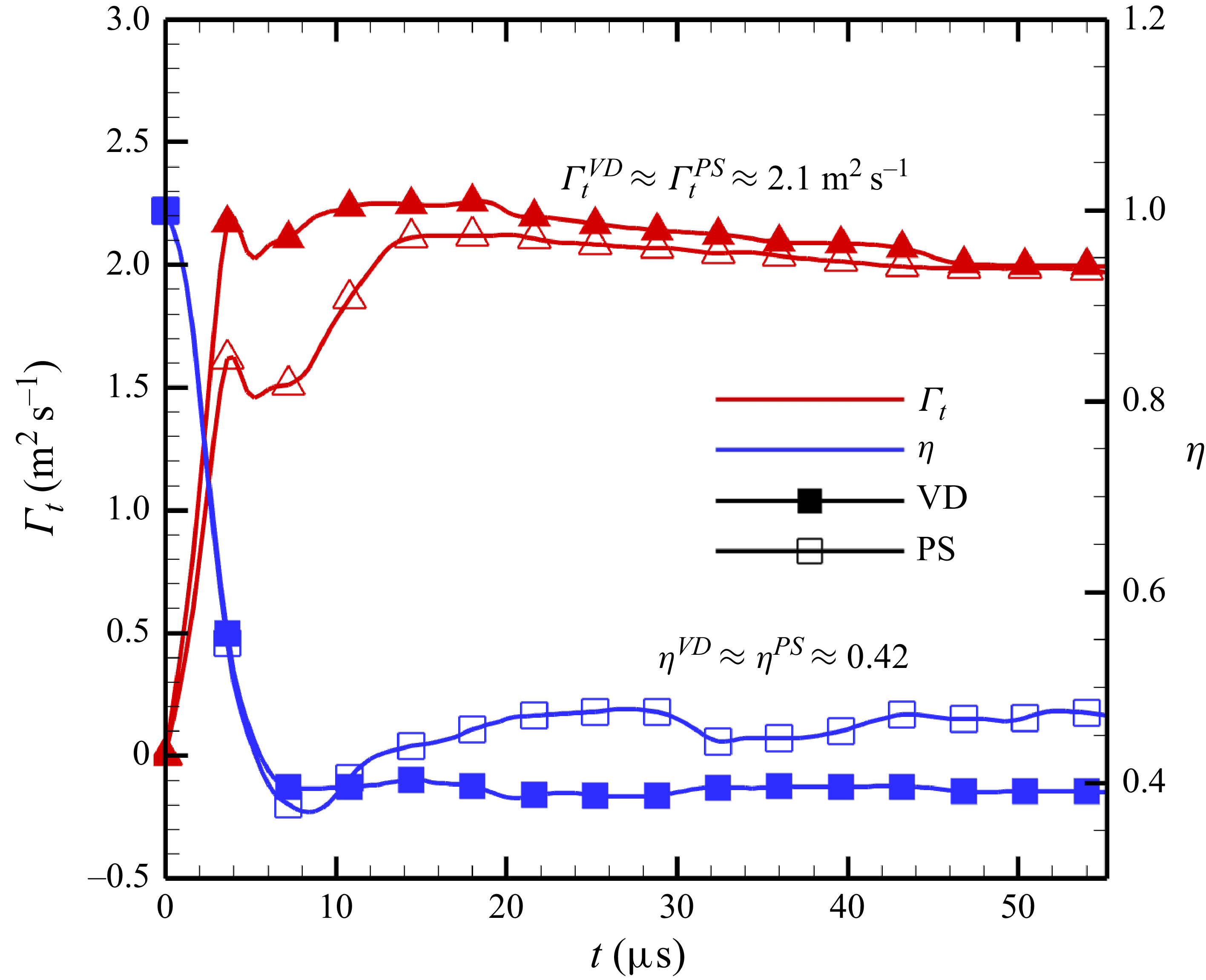in the later stage of VD SBI. Figure 3 illustrates the evolution of $\varGamma _{t}$ and $\eta$ in both VD and PS SBI cases. Following the shock interaction with the bubble, both the total circulation $\varGamma _t$ and the compression rate $\eta$ converge to nearly constant values, indicating the formation of a nearly steady single vortex. It is also observed that the total circulation $\varGamma _t$ in both the PS and VD SBI cases is nearly identical. Although the compression rate in the PS SBI case is approximately 20 $\%$ greater than in the VD SBI case, the impact of this small difference in $\eta$ on the subsequent discussions is negligible. Therefore, the compression rate $\eta$ can be considered a consistent value of 0.42 for both the PS and VD SBI cases. Consequently, both the total circulation $\varGamma _t$ and the compression rate $\eta$ are unaffected by the specific settings of the PS SBI case. Furthermore, due to the conservation of the total circulation $\varGamma _{t}$ and the alteration in bubble density in the PS SBI, the dynamic viscosity is adjusted to maintain the same dimensionless Reynolds number ${\textit{Re}} = \varGamma _{t}/\nu$ . This modification is expressed as $\mu ^{\textit{ps}} = \mu ^{\textit{VD}}( {2\rho _{2}'}/({\rho _{1}' + \rho _{2}'}))$ , ensuring the kinematic viscosity $\nu = \mu / \overline {\rho '}$ remains constant. The maintenance of ${\textit{Pe}} = \varGamma _{t}/\mathcal{D}$ is achieved by keeping the same Fickian diffusivity $\mathcal{D}$ . The set-up for the PS SBI case is summarised in table 1.

Figure 3.

Comparison of the total circulation $\varGamma _{t}$ and compression rate $\eta$ between the PS and VD SBI cases at a shock Mach number of 2.4.

Table 1.

The set-up for the PS SBI case based on the VD SBI case with a shock Mach number of ${\textit{Ma}} = 2.4$ . Compared with VD SBI, the post-shock parameters $p_{1}^{\prime}$ , $T_{1}^{\prime}$ , $u_{1}^{\prime}$ and $T_{1}^{\prime}$ in PS SBI remain unchanged, while the Atwood number, reflecting the post-shock density difference, is set to zero $(At^{+} = 0)$ . With the total circulation $\varGamma _{t}$ preserved, the Péclet number is maintained, and the Reynolds number ${\textit{Re}}$ is held constant by adjusting the dynamic viscosity $\mu$ in the PS SBI case.

The reduction of SBV due to the absence of density differences is a primary characteristic of PS mixing. Another feature of PS mixing is that the evolution of the mass fraction $Y$ follows the advection–diffusion equation (Warhaft Reference Warhaft2000), expressed as

(2.14) \begin{equation} \frac{\partial Y}{\partial t} + \frac{\partial (u_i Y)}{\partial x_i} = \mathcal{D}\frac{\partial ^2 Y}{\partial {x_{\!j}}^2}. \end{equation}

Here, the absence of density differences also leads to the reduction of the multi-component transport equation in (2.1) to the advection–diffusion equation, indicating a shift from a VD mixing characteristic to a PS mixing characteristic. As shown in (2.1), the multi-component transport equation for the mass fraction of helium $Y$ is expressed as

(2.15) \begin{equation} \frac{\partial(\rho Y)}{\partial t} + \frac{\partial (\rho u_i Y)}{\partial x_i} = \frac{\partial }{\partial x_{\!j}}\left (\rho \mathcal{D} \frac{\partial Y}{\partial x_{\!j}}\right )\!. \end{equation}

Since the Fickian diffusivity $\mathcal{D}$ is treated as constant in our numerical simulations, this equation can be rewritten in the form VD advection–diffusion equation

(2.16) \begin{equation} \frac{\partial Y}{\partial t} + \frac{\partial ( u_i Y)}{\partial x_i} = \frac{\mathcal{D}}{\rho }\left (\frac{\partial \rho }{\partial x_{\!j}}\frac{\partial Y}{\partial x_{\!j}}\right ) + \mathcal{D}\frac{\partial ^2 Y}{\partial x_{\!j}^2}. \end{equation}

When the density gradient $ {\partial \rho }/{\partial x_{\!j}}$ vanishes in the PS SBI, this equation reduces to the standard advection–diffusion equation.

In summary, the PS SBI set-up transforms the VD SBI into a system with two key PS mixing characteristics: (i) the disappearance of SBV during the development of the single vortex, and (ii) the reduction of the multi-component transport equation to the advection–diffusion equation. These two features facilitate the development of a quantitative theory for describing the stretching dynamics and its impact on mixing, which will be presented in the following sections.

3.1. Importance of the stretching term to SDR evolution in SBI

To explore the role of the stretching dynamics in mixing for PS and VD SBI, it is essential to define the stretching rate within an appropriate framework. Following previous studies on PS mixing (Cetegen & Mohamad Reference Cetegen and Mohamad1993; Buch & Dahm Reference Buch and Dahm1996), the SDR, denoted as $\chi$ and defined in (1.3), serves as a suitable mixing indicator for this purpose. The definition and physical interpretation of SDR stem from another mixing indicator, the mixedness parameter $f$ defined in (1.1). This parameter quantifies the extent of mixing, and reaches its maximum when the mass fractions of the bubble’s relevant component and the surrounding air are equal.

Figure 4.

Time evolution of the mixedness contour (top) and the SDR contour (bottom) for VD SBI case with shock Mach number 2.4 at $(a)\ t=10.8\ \rm {\unicode {x03BC} s}$ ; $(b)\ t=21.6\ \rm {\unicode {x03BC} s}$ ; $(c)\ t=32.4\ \rm {\unicode {x03BC} s}$ ; $(d)\ t=43.2\ \rm {\unicode {x03BC} s}$ ; and $(e)\ t=54.0\ \rm {\unicode {x03BC} s}$ . The PS SBI case is presented at the same moments as those of VD SBI in the bottom from $(f)$ to $(j)$ . Red dashed-dot line indicates the isoline of $Y = 0.01$ .

Figure 5.

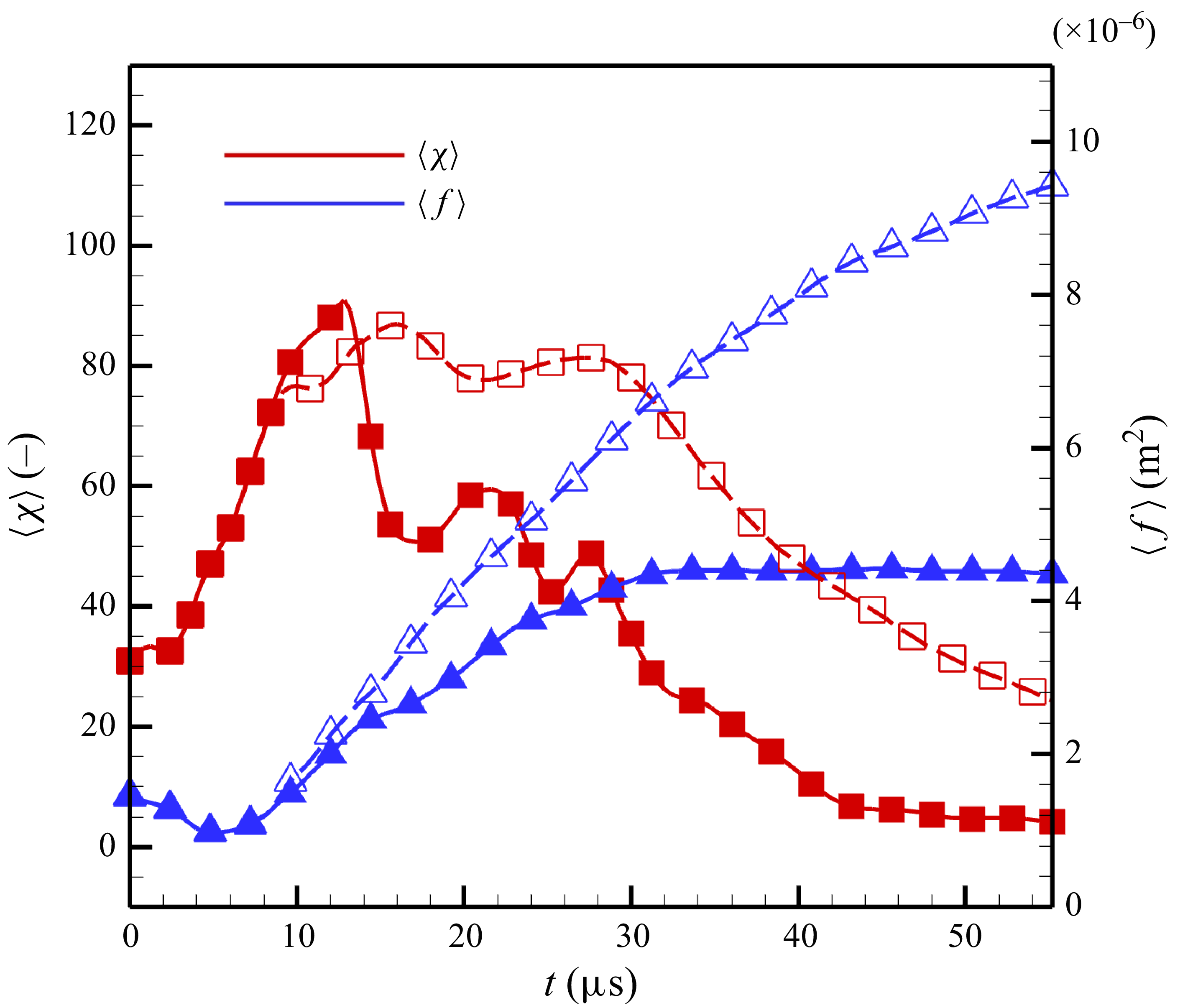
Time evolution of the total mixedness (blue) and SDR (red) for PS and VD SBI cases demonstrated in figure 4, respectively. The solid line labels the VD SBI, while the dashed line indicates the PS SBI.

Following the definition of mixedness and based on (2.15), the behaviour of mixedness $f$ is governed by the following equation:

(3.1) \begin{equation} \left (\frac{\partial }{\partial t} + u_{\!j} \frac{\partial }{\partial x_{\!j}} - \mathcal{D}\frac{\partial ^2}{\partial x_{\!j}^2}\right )f = 8\mathcal{D}\frac{\partial Y}{\partial x_{\!j}}\frac{\partial Y}{\partial x_{\!j}}+4\left (1-2Y\right )\frac{\mathcal{D}}{\rho }\frac{\partial \rho }{\partial x_{\!j}}\frac{\partial Y}{\partial x_{\!j}}. \end{equation}

The first term on the right-hand side is strictly positive, representing the growth rate of mixedness. Thus the definition of SDR $\chi = ({\partial Y}/{\partial x_i}) ({\partial Y}/{\partial x_i}) $ reflects the physical meaning of mixing rate. The second term originates from the density gradient $ {\partial \rho }/{\partial x_i}$ , and vanishes in PS SBI due to the disappearance of density difference.

Figure 4 illustrates the temporal evolution of both mixedness and SDR in PS and VD SBI. As the initially concentrated bubble undergoes the stretching process, the SDR initially increases, subsequently decreases at the later stages and ultimately dissipates, indicating the achievement of a well-mixed state. Different from the behaviour of SDR, the general trend of the mixedness is monotonically increasing. The evolution processes of these two mixing indicators (1.1 and (1.3)) can be described in detail by examining their total values, which are defined by the corresponding volume integrations

(3.2) \begin{equation} \left \{ \!\!\!\begin{aligned} & \left \langle f \right \rangle = \iint _{\mathcal{V}} f \rm {dV},\\ & \left \langle \chi \right \rangle = \iint _{\mathcal{V}} \chi \rm {dV}. \end{aligned} \right . \end{equation}

As shown in figure 5, the mixedness in both PS and VD SBI increases monotonically. In contrast, the SDR initially increases and then decreases after a certain moment. Another notable observation from this figure is that, despite the total circulation $\varGamma _{t}$ and compression rate $\eta$ being consistent between PS SBI and VD SBI, there is a significant difference in the total mixedness $\langle f\rangle$ and the total SDR $\langle \chi \rangle$ between the two cases. This phenomenon arises from the discrepancy between the mixing mechanism in PS and VD mixing flow, which will be exhibited further in the following sections.

To gain further insight into the underlying mechanisms driving these two mixing indicators, it is necessary to derive the corresponding governing equations. For the mixedness equation, using the mathematical expression for the time derivative of the volumetric mean value (Yu et al. Reference Yu, Liu and Liu2021), we have

(3.3) \begin{equation} \frac{{\textrm {D}} \langle f \rangle }{{\textrm {D}}t} = \left \langle \frac{{\textrm {D}} f}{{\textrm {D}}t} \right \rangle + \left \langle \left (\frac{\partial u_i}{\partial x_i}\right ) \! f\right \rangle\! , \end{equation}

which leads to the governing equation for the total mixedness $\langle f \rangle$ as

(3.4) \begin{equation} \frac{{\textrm {D}} \langle f \rangle }{{\textrm {D}}t} = \left \langle 8\mathcal{D}\frac{\partial Y}{\partial x_{\!j}}\frac{\partial Y}{\partial x_{\!j}} \right \rangle + \left \langle 4\left (1-2Y\right )\frac{\mathcal{D}}{\rho }\frac{\partial \rho }{\partial x_{\!j}}\frac{\partial Y}{\partial x_{\!j}}\right \rangle + \left \langle - \left (\frac{\partial u_i}{\partial x_i}\right )\! f\right \rangle . \end{equation}

Subsequently, the source of total mixedness growth $\Delta \left\langle f \right\rangle =\left\langle f \right\rangle|_t - \left\langle f \right\rangle|_0$ can be decomposed by considering the absence of mixedness transport across the boundaries of the integration region, specifically $\langle \mathcal{D}({\partial ^2 f}/{\partial x_{\!j}^2}) \rangle = 0$ . This decomposition is described as follows:

(3.5) \begin{equation} \left \{ \begin{aligned} & \varDelta \langle f \rangle = \left \langle T_{\textit{SDR}}^{f} \right \rangle + \left \langle T_{den}^{f} \right \rangle + \left \langle T_{\textit{divU}}^{f} \right \rangle\! ,\\& \left \langle T_{\textit{SDR}}^{f} \right \rangle = \int _{0}^{t}\left \langle 8\mathcal{D}\frac{\partial Y}{\partial x_{\!j}}\frac{\partial Y}{\partial x_{\!j}} \right \rangle {\textrm {d}}t',\\& \left \langle T_{den}^{f} \right \rangle = \int _{0}^{t} \left \langle 4\left (1-2Y\right )\frac{\mathcal{D}}{\rho }\frac{\partial \rho }{\partial x_{\!j}}\frac{\partial Y}{\partial x_{\!j}}\right \rangle {\textrm {d}}t', \\& \left \langle T_{\textit{divU}}^{f} \right \rangle = \int _{0}^{t} \left \langle - \left (\frac{\partial u_i}{\partial x_i}\right )\!f\right \rangle {\textrm {d}}t', \end{aligned} \right . \end{equation}

where $\langle T_{\textit{SDR}}^{f} \rangle$ is the SDR source term, $ \langle T_{den}^{f} \rangle$ is the density-gradient source term and $\langle T_{\textit{divU}}^{f} \rangle$ is the velocity-divergence source term. Similar to the total mixedness equation in (3.4), the governing equation for the total SDR can also be derived based on (2.15) as

(3.6) \begin{equation} \left \{ \begin{aligned} & \frac{{\textrm {D}}\left \langle \chi \right \rangle }{{\textrm {D}}t} = \left \langle T_{\textit{stretch}}^{\chi } \right \rangle + \left \langle T_{\textit{diff}}^{\chi } \right \rangle + \left \langle T_{\textit{source}}^{\chi } \right \rangle + \left \langle T_{\textit{divU}}^{\chi } \right \rangle\! ,\\ & \left \langle T_{\textit{stretch}}^{\chi } \right \rangle = \left \langle -2\frac{\partial Y}{\partial x_i} S_{\textit{ij}} \frac{\partial Y}{\partial x_{\!j}}\right \rangle\! ,\\ & \left \langle T_{\textit{diff}}^{\chi } \right \rangle = \left \langle -2\mathcal{D}\frac{\partial }{\partial x_i}\left (\frac{\partial Y}{\partial x_{\!j}}\right )\frac{\partial }{\partial x_i}\left (\frac{\partial Y}{\partial x_{\!j}}\right )\right \rangle\! , \\ & \left \langle T_{\textit{source}}^{\chi } \right \rangle = \left \langle 2\mathcal{D}\frac{\partial Y}{\partial x_i}\frac{\partial }{\partial x_i}\left (\frac{1}{\rho }\frac{\partial \rho }{\partial x_{\!j}}\frac{\partial Y}{\partial x_{\!j}}\right ) \right \rangle\! , \\ & \left \langle T_{\textit{divU}}^{\chi } \right \rangle = \left \langle -\left (\frac{\partial u_i}{\partial x_i}\right ) \chi \right \rangle\! , \end{aligned} \right . \end{equation}

where $\langle T_{\textit{stretch}}^{\chi } \rangle$ is the stretching term expressed as the combination of the scalar gradient $ {\partial Y}/{\partial x_i}$ and the symmetric strain-rate tensor $S_{\textit{ij}}= {1}/{2}( {\partial u_{i}}/{\partial x_{\!j}} + {\partial u_{\!j}}/{\partial x_i})$ , $ \langle T_{\textit{diff}}^{\chi } \rangle$ is the diffusion term, $\langle T_{\textit{source}}^{\chi } \rangle$ is the density-gradient source term and $\langle T_{\textit{divU}}^{\chi } \rangle$ is the velocity-divergence source term.

Figure 6.

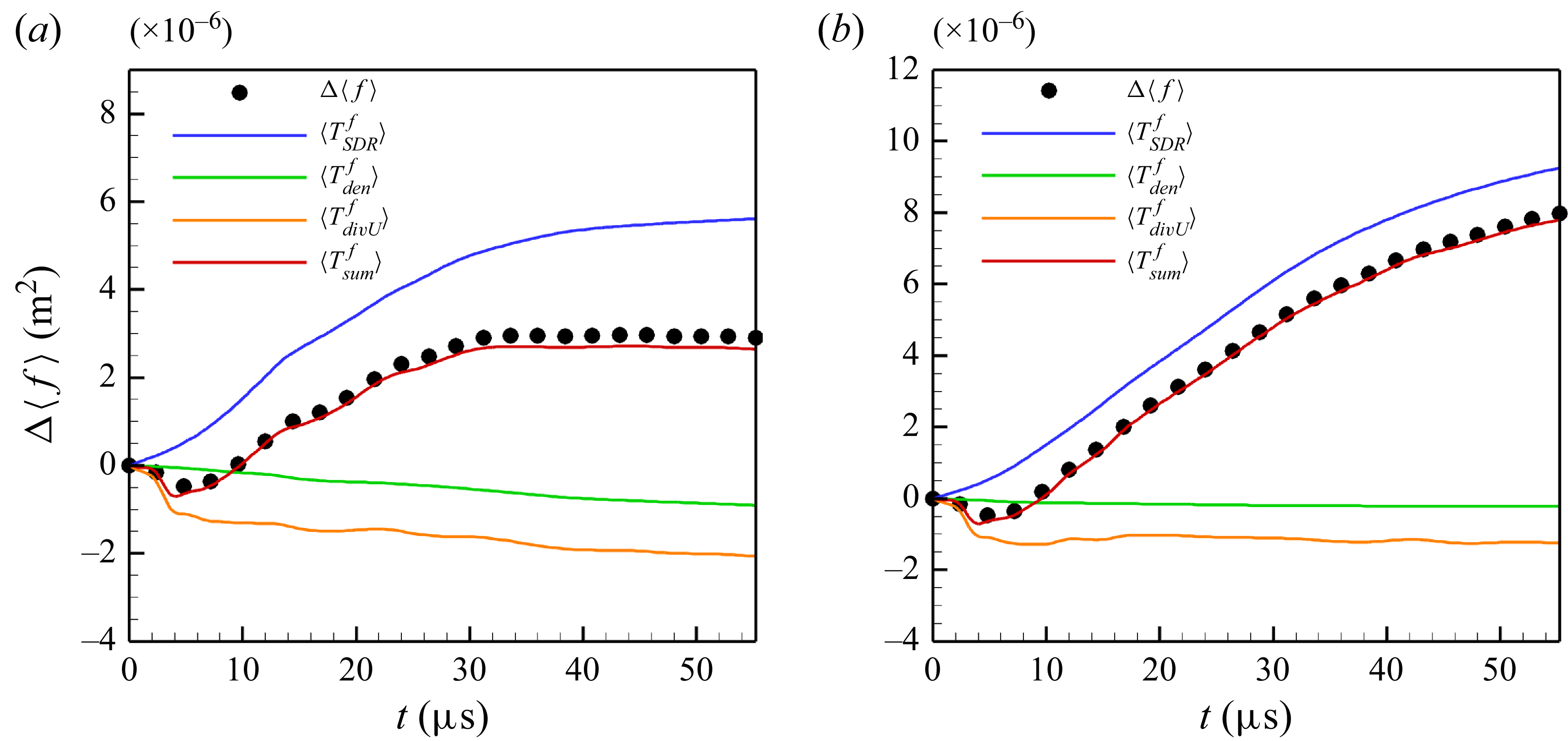
The decomposition of the total mixedness growth $\Delta \langle f \rangle$ in (3.5) for $(a)$ VD SBI and $(b)$ PS SBI. The black symbols refers to the increment of the total mixedness $\Delta \langle f \rangle$ , which is calculated from the corresponding evolution of $\langle f \rangle$ in figure 5. The red solid line indicates the summation of the terms on the right side of (3.5) $\langle T_{sum}^{f} \rangle$ .

Figure 7.

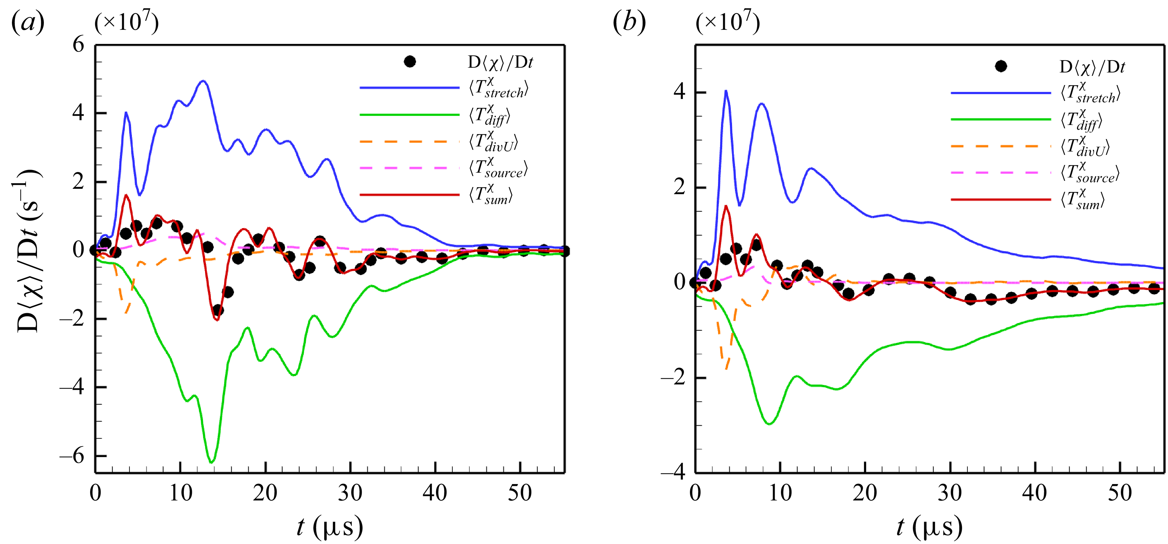
The decomposition of the material derivative of the total SDR growth $ {{\textrm {D}}\langle \chi \rangle }/{{\textrm {D}}t}$ in (3.6) for $(a)$ VD SBI and $(b)$ PS SBI. The black symbols refers to the material derivative of the total SDR growth $ {{\textrm {D}}\langle \chi \rangle }/{{\textrm {D}}t}$ , which is obtained from the evolution of $\langle\chi\rangle$ in figure 5. The red solid line indicates the summation of the terms on the right side of (3.6) $\langle T_{sum}^{\chi } \rangle$ .

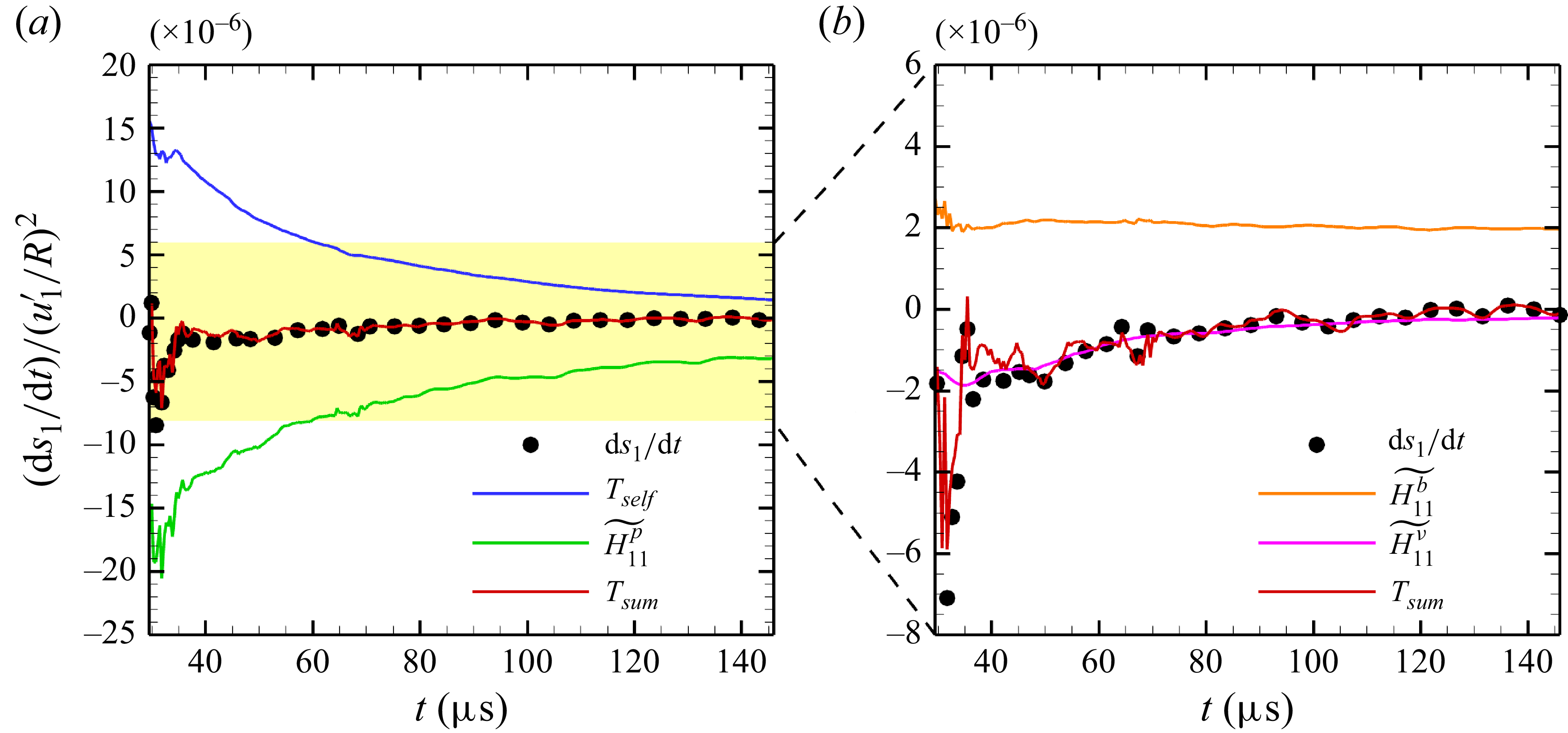
We begin by analysing the decomposition of the total mixedness growth $\Delta \langle f \rangle$ as expressed in (3.5). As shown in figure 6, the initial decrease in total mixedness $\Delta \langle f \rangle$ arises from the velocity-divergence source term $\langle T_{\textit{divU}}^{f} \rangle$ in both PS and VD SBI cases, reflecting the effect of shock compression. The primary driver of the monotonic increase in total mixedness, however, is the SDR source term $\langle T_{\textit{SDR}}^{f} \rangle$ . These findings from the decomposition of total mixedness growth confirm that the SDR $\chi$ accurately represents the physical mixing rate and underscore that the growth of mixedness can be almost represented by the SDR source term, which is defined by the time integration of the SDR.

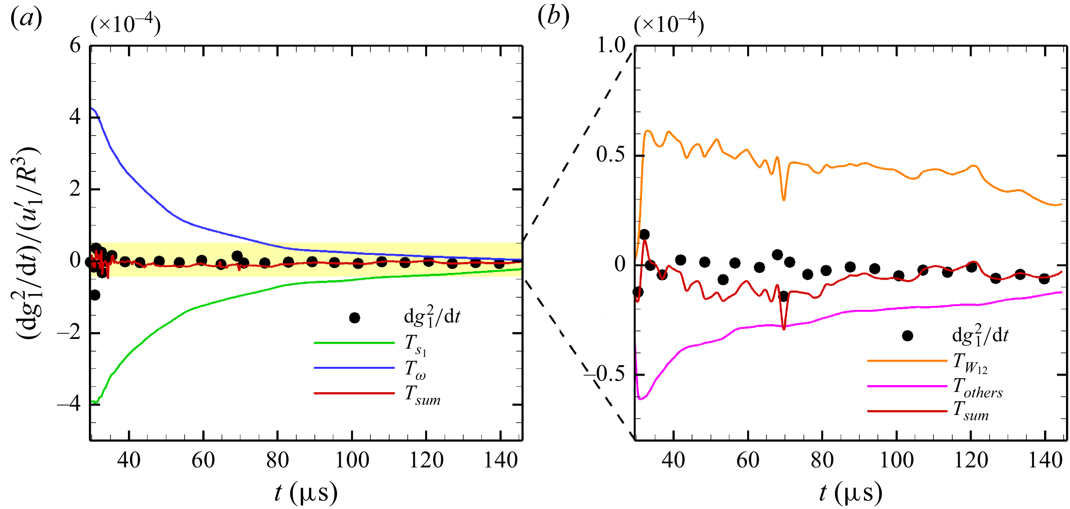
Furthermore, the governing equation for the SDR in (3.6) is analysed in figure 7. Consistent with previous studies (Danish et al. Reference Danish, Suman and Girimaji2016; Tian et al. Reference Tian, Jaberi, Li and Livescu2017; Gao et al. Reference Gao, Bermejo-Moreno and Larsson2020), the stretching term $\langle T_{\textit{stretch}}^{\chi }\rangle$ serves as the primary contributor to SDR growth, while the strictly negative diffusion term $\langle T_{\textit{diff}}^{\chi } \rangle$ is the predominant factor in SDR reduction. In comparison, the effects of the density-gradient source term $\langle T_{\textit{source}}^{\chi } \rangle$ and the velocity-divergence source term $\langle T_{\textit{divU}}^{\chi } \rangle$ on SDR are nearly negligible. This observation highlights that the evolution of SDR is governed by the coupled interaction of stretching dynamics and diffusion processes. Therefore, understanding the SDR necessitates a focus on the stretching dynamics, with the stretching term defined rigorously within this framework: $T_{\textit{stretch}}^{\chi } = -2 ({\partial Y}/{\partial x_i}) S_{\textit{ij}}({\partial Y}/{\partial x_{j}}) $ .

3.2. Stretching dynamics governing equations (SDGEs)

To further explore the stretching dynamics, according to the symmetry of the strain-rate tensor $S_{\textit{ij}}$ , the stretching term can be decomposed within an orthogonal strain-rate eigenframe, which consists of the principal strain rates $s_i$ and their corresponding eigenvectors $\boldsymbol{e}_i$ . The orthogonal expression of the stretching term is provided by (1.5): $T_{\textit{stretch}}^{\chi } = -2\chi s_i \lambda _{i}^2$ , indicating that the stretching term $T_{\textit{stretch}}^{\chi }$ is influenced by both the principal strain rates $s_i$ and the alignment of the scalar gradient with the corresponding eigenvectors $\lambda _i = \boldsymbol{\nabla }Y \boldsymbol{\cdot }\boldsymbol{e}_i/|\boldsymbol{\nabla }Y|$ . Consequently, the stretching rate is defined as the product of the principal strain rate $s_i$ and the scalar gradient alignment $\lambda _i$ as described in (1.6): $R_{\textit{stretch}} = -2 s_i \lambda _i^2$ .

Analysing the stretching rate $R_{\textit{stretch}}$ from the perspective of the stretching dynamics requires the governing equations for the principal strain rate $s_i$ and the alignment of the scalar gradient $\lambda _i$ . These two equations can be derived by taking the gradient of the momentum equation in (2.1) and the multi-component transport equation in (2.15), and projecting them onto the strain-rate eigenframe (Dresselhaus & Tabor Reference Dresselhaus and Tabor1992; Ohkitani & Kishiba Reference Ohkitani and Kishiba1995; Tom et al. Reference Tom, Carbone and Bragg2021; Han et al. Reference Han, Yu and Liu2024). Details of these derivations are provided in the supplementary material are available at https://doi.org/10.1017/jfm.2025.11051. We refer to the principal strain-rate equations as the SDGEs for $s_i$ (SDGE- $s_i$ ), which are expressed as follows:

(3.7) \begin{equation} \left \{ \begin{aligned} &\frac{\textrm {d}}{{\textrm {d}} t}s_i = -s_{i}^2 - \frac{1}{4}\left ({\widetilde {\omega _i}}^2 - \omega ^2\right ) + \widetilde {H_{\textit{ii}}^p} + \widetilde {H_{\textit{ii}}^b} + \widetilde {H_{\textit{ii}}^{\nu }},\\ &\left (s_{\!j} - s_i\right )\widetilde {W_{\textit{ij}}} = -\frac{1}{4}\widetilde {\omega _i}\widetilde {\omega _{\!j}} + \widetilde {H_{\textit{ij}}^p} + \widetilde {H_{\textit{ij}}^b} + \widetilde {H_{\textit{ij}}^{\nu }},\\ &\frac{\textrm {d}}{{\textrm {d}}t}\widetilde {\omega _{i}} = s_i \widetilde {\omega _i} - \left (\frac{\partial u_i}{\partial x_i}\right )\widetilde {\omega _i} + \widetilde {B_i} + \widetilde {T_i^{\nu }} - \widetilde {\omega _{\!j}}\widetilde {W_{\textit{ij}}}, \end{aligned} \right . \end{equation}

In the first of these equations, $s_i$ represents the principal strain rate, $\widetilde {\omega _{i}} = \boldsymbol{e}_i^{T} \boldsymbol{\cdot }\boldsymbol{\omega }$ are the vorticity components in the strain eigenframe, where $\boldsymbol{\omega } = \boldsymbol{\nabla }\times \boldsymbol{u}$ is the vorticity vector. The norm of the vorticity vector is given by $\omega = ||\boldsymbol{\omega }||$ . The terms $H_{\textit{ij}}^{p} = - {1}/{\rho }({\partial ^2 p}/{\partial x_i \partial x_{\!j}}) $ , $H_{\textit{ij}}^{b} = {1}/({2\rho ^2}) (({\partial \rho }/{\partial x_i}) ({\partial p}/{\partial x_{\!j}}) + ({\partial \rho }/{\partial x_{\!j}}) ( {\partial p}/{\partial x_i}) )$ and $H_{\textit{ij}}^{\nu }= {1}/{2} [ {\partial }/{\partial x_{\!j}} (({1}/{\rho }) {\partial \sigma _{ik}}/{\partial x_k} ) + {\partial }/{\partial x_i} (({1}/{\rho }) {\partial \sigma _{jk}}/{\partial x_k} ) ]$ correspond to the pressure Hessian, baroclinic strain and viscous stress matrix, respectively. The notation $\widetilde { ( )}$ denotes the projection of these matrices onto the strain eigenframe, calculated as

(3.8) \begin{equation} \widetilde {H_{\textit{ij}}^{p}} = \boldsymbol{e}_{i}^T \boldsymbol{H}^{p} \boldsymbol{e}_{\!j},\qquad \widetilde {H_{\textit{ij}}^{b}} = \boldsymbol{e}_{i}^T \boldsymbol{H}^{b} \boldsymbol{e}_{\!j},\qquad \widetilde {H_{\textit{ij}}^{\nu }} = \boldsymbol{e}_{i}^T \boldsymbol{H}^{\nu } \boldsymbol{e}_{\!j}. \end{equation}

In the second equation, $\widetilde {W_{\textit{ij}}}$ characterises the rate of rotation within the plane formed by two eigenvectors about the axis of the third one, that is $\widetilde {W_{\textit{ij}}} = ({\textrm {d}}/{{\textrm {d}}t}) \boldsymbol{e}_{\!j} \boldsymbol{\cdot }\boldsymbol{e}_{i}$ . The third equation pertains to the vorticity dynamics, where $\widetilde {B_i}$ and $\widetilde {T_i^{\nu }}$ represent the projections of the baroclinic vorticity $B_{i} = \epsilon _{\textit{ijk}}({1}/{\rho ^2}) ({\partial \rho }/{\partial x_{\!j}}) ({\partial p}/{\partial x_k}) $ and the viscous contribution $T_{i}^{\nu } = \epsilon _{\textit{ijk}}({\partial }/{\partial x_{\!j}}) (({1}/{\rho }) ({\partial \sigma _{kn}}/{\partial x_n}) )$ onto the strain eigenframe, expressed as

(3.9) \begin{equation} \widetilde {B_i} = \boldsymbol{e}_{i}^{T}\boldsymbol{B},\qquad \widetilde {T_i^{\nu }} = \boldsymbol{e}_{i}^{T}\boldsymbol{T^{\nu }}, \end{equation}

where $\epsilon _{\textit{ijk}}$ is the permutation symbol.

The SDGE for $\lambda _i$ (SDGE- $\lambda _i$ ) pertains to the alignment of the scalar gradient $\lambda _{i}$ , and is formulated as follows:

(3.10) \begin{equation} \frac{\textrm {d}}{{\textrm {d}}t}\lambda _i = -s_i\lambda _i + \xi _{\textit{stretch}}\lambda _{i} - \widetilde {W_{\textit{ij}}}\lambda _{\!j} + \frac{1}{2}\epsilon _{\textit{ijk}}\widetilde {\omega _{\!j}}\lambda _{k} + \frac{1}{\sqrt {\chi }}T_{i}^{\textit{others}}, \end{equation}

where $\xi _{\textit{stretch}} = s_{i}\lambda _{i}^2$ represents the stretching contribution, and $({1}/{\sqrt {\chi }})T_{i}^{\textit{others}}$ characterises the diffusion effect. Due to the presence of the square root of SDR in the denominator of the diffusion effect, 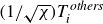$({1}/{\sqrt {\chi }})T_{i}^{\textit{others}}$ can generally be neglected in the context of flow structures with a large SDR value. This simplification is justified and demonstrated in Appendix C.

By focusing on the principal strain $s_i$ and the scalar gradient alignment $\lambda _i$ , the framework for the stretching dynamics, which centres on the stretching rate $R_{\textit{stretch}} = -2 s_{i} \lambda _{i}^2$ , can be comprehensively described through the combination of SDGE- $s_i$ and SDGE- $\lambda _i$ . The validity of the framework is corroborated through Lagrangian methods, as detailed in Appendix C.

3.3. Analytical solution of SDGEs in a single vortex

Motivated by the formation of a nearly steady single vortex following the shock’s interaction with the bubble, as depicted in figure 2, this subsection investigates the stretching dynamics within a single vortex. This research is conducted by solving the SDGEs analytically in a cylindrical coordinate system $(r, \varphi )$ , where the centre of the main vortex serves as the origin. In this context, $r$ represents the radial direction, while $\varphi$ indicates the azimuthal direction. To facilitate the simplification of the SDGEs, several assumptions and observations regarding vortex morphology for PS mixing are introduced:

Assumption PS.(i) The single vortex is axisymmetric in the azimuthal direction $\varphi$ , with negligible radial velocity, implying ${\partial }/{\partial \varphi } = 0$ and $u_r = 0$ . This assumption simplifies the momentum equation in (2.1) to $- {u_{\varphi }^2}/{r} = -({1}/{\rho }) {\partial p}/{\partial r}$ .

Assumption PS.(ii) Following the shock interaction, the single vortex is considered incompressible, aligning with previous research on RMI (Peng et al. Reference Peng, Yang, Wu and Xiao2021a ).

Assumption PS.(iii) The density gradient within the single vortex is negligible, i.e. $\boldsymbol{\nabla }\rho = 0$ .

Assumption PS.(iv) The mixing of PS SBI can be approximated as the mixing of a compressed semicircle composed of a series of scalar strips, each undergoing deformation due to the continuous stretching effect of the single vortex.

The validation of these assumptions is provided in the supplementary materials. Under assumptions PS.(i) and two-dimensional flow conditions, the SDGE- $s_i$ presented in (3.7) can be simplified by expressing these equations in cylindrical coordinates as follows:

(3.11) \begin{equation} \left \{ \begin{aligned} &\frac{\textrm {d}}{{\textrm {d}}t}s_1 = -\frac{1}{2\rho ^2}\frac{1}{r}\frac{\partial \rho }{\partial \varphi }\frac{\partial p }{\partial r} + \nu \left (\frac{\partial ^2 s_1}{\partial r^2} + \frac{1}{r}\frac{\partial s_1}{\partial r}\right )\!,\\ &\frac{\textrm {d}}{{\textrm {d}}t}s_2 = \frac{1}{2\rho ^2}\frac{1}{r}\frac{\partial \rho }{\partial \varphi }\frac{\partial p }{\partial r} + \nu \left (\frac{\partial ^2 s_2}{\partial r^2} + \frac{1}{r}\frac{\partial s_2}{\partial r}\right )\!,\\ &\widetilde {W_{12}}\approx \frac{\widetilde {H_{12}^p} + \widetilde {H_{12}^b}}{s_2 - s_1} = -\frac{u_{\varphi }}{r},\\ & \frac{\textrm {d}}{{\textrm {d}}t}\omega = -\frac{1}{2\rho ^2}\frac{1}{r}\frac{\partial \rho }{\partial \varphi }\frac{\partial p }{\partial r} + \nu \left (\frac{\partial ^2 s_1}{\partial r^2} + \frac{1}{r}\frac{\partial s_1}{\partial r}\right )\!. \end{aligned} \right . \end{equation}

In these equations, with assumption PS.(ii), $s_1$ and $s_2$ , representing the positive and negative principal strain rate, respectively, satisfy the relation $s_1 + s_2 = 0$ . Additionally, $\omega$ denotes the vorticity magnitude perpendicular to the plane of the two-dimensional single vortex. Furthermore, these equations can be further simplified under assumption PS.(iii) by ignoring the density gradient $\boldsymbol{\nabla }\rho$

(3.12) \begin{equation} \left \{ \begin{aligned} &\frac{\textrm {d}}{{\textrm {d}}t}s_1 = \nu \left (\frac{\partial ^2 s_1}{\partial r^2} + \frac{1}{r}\frac{\partial s_1}{\partial r}\right )\!,\\ &\frac{\textrm {d}}{{\textrm {d}}t}s_2 = \nu \left (\frac{\partial ^2 s_2}{\partial r^2} + \frac{1}{r}\frac{\partial s_2}{\partial r}\right )\!,\\ &\widetilde {W_{12}}\approx \frac{\widetilde {H_{12}^p} + \widetilde {H_{12}^b}}{s_2 - s_1} = -\frac{u_{\varphi }}{r},\\ & \frac{\textrm {d}}{{\textrm {d}}t}\omega = \nu \left (\frac{\partial ^2 s_1}{\partial r^2} + \frac{1}{r}\frac{\partial s_1}{\partial r}\right )\!. \end{aligned} \right . \end{equation}

These equations suggest that the principal strain rate $s_i$ and the associated parameters are primarily governed by the viscous effects.

Given the constant total circulation $\varGamma _{t}$ depicted in figure 3, the analytical solution of (3.12) can be expressed as

(3.13) \begin{equation} \left \{ \begin{aligned} & s_1 = \frac{1}{2}\left (-\frac{\partial u_{\varphi }}{\partial r} + \frac{ u_{\varphi }}{r}\right ) = \frac{\varGamma _{t}}{2\pi r^2}\left (1-{\textrm {exp}}\left (-\frac{r^2}{4\nu t}\right )\right ) - \frac{\varGamma _{t}}{8\pi \nu t}{\textrm {exp}}\left (-\frac{r^2}{4\nu t}\right )\!,\\ & \widetilde {W_{12}} = -\frac{u_{\varphi }}{r} = -\frac{\varGamma _{t}}{2\pi r^2}\left (1-{\textrm {exp}}\left (-\frac{r^2}{4\nu t}\right )\right )\!,\\ & \omega = \frac{\partial u_{\varphi }}{\partial r} + \frac{u_{\varphi }}{r} = \frac{\varGamma _t}{4\pi \nu t}{\textrm { exp}}\left (-\frac{r^2}{4\nu t}\right )\!,\\ & \boldsymbol{e}_1 = \left ( \cos \left (-\frac{\pi }{4} + \varphi \right )\!, \sin \left (-\frac{\pi }{4} + \varphi \right )\right )\!. \end{aligned} \right . \end{equation}

This solution derived for the principal strain rate $s_i$ within a single vortex aligns well with the principal strain rate obtained from Saffman’s viscous vortex ring model (Saffman Reference Saffman1970), given by

(3.14) \begin{equation} u_{\varphi } = \frac{\varGamma _{t}}{2\pi r}\left (1-{\textrm {exp}}\left (-\frac{r^2}{4\nu t}\right )\right )\!. \end{equation}

For the scalar gradient alignment $\lambda _i$ , SDGE- $\lambda _i$ as represented in (3.10) can be firstly simplified under two-dimensional flow condition

(3.15) \begin{equation} \left \{ \begin{aligned} & \frac{\textrm {d}}{{\textrm {d}}t}\lambda _1 = -\left (s_1 - s_2\right )\left (\lambda _1\lambda _2^2 + \frac{\widetilde {W_{12}} + \omega /2}{s_1-s_2}\lambda _2\right )+\frac{1}{\sqrt {\chi }}T_1^{\textit{others}},\\ & \frac{\textrm {d}}{{\textrm {d}}t}\lambda _2 = \left (s_1 - s_2\right )\left (\lambda _1^2\lambda _2 + \frac{\widetilde {W_{12}} + \omega /2}{s_1-s_2}\lambda _1\right )+\frac{1}{\sqrt {\chi }}T_2^{\textit{others}}. \end{aligned} \right . \end{equation}

Moreover, in a two-dimensional flow, the alignment of the scalar gradient $\lambda _i$ satisfies the relation $\lambda _1^2 + \lambda _2^2 = 1$ . Therefore, using the triangular transformation

(3.16) \begin{equation} \lambda _1 = \cos \theta ,\qquad \lambda _2 = \sin \theta . \end{equation}

Equation (3.15) can be further simplified by neglecting the high-order terms $(1/\sqrt{\chi})T_i^{\textit{others}}$ in the flow structures with a large SDR value, shown as

(3.17) \begin{equation} \frac{\textrm {d}}{{\textrm {d}}t}\theta = \frac{s_1- s_2}{2}\left (\sin 2\theta + \xi \right )\!, \end{equation}

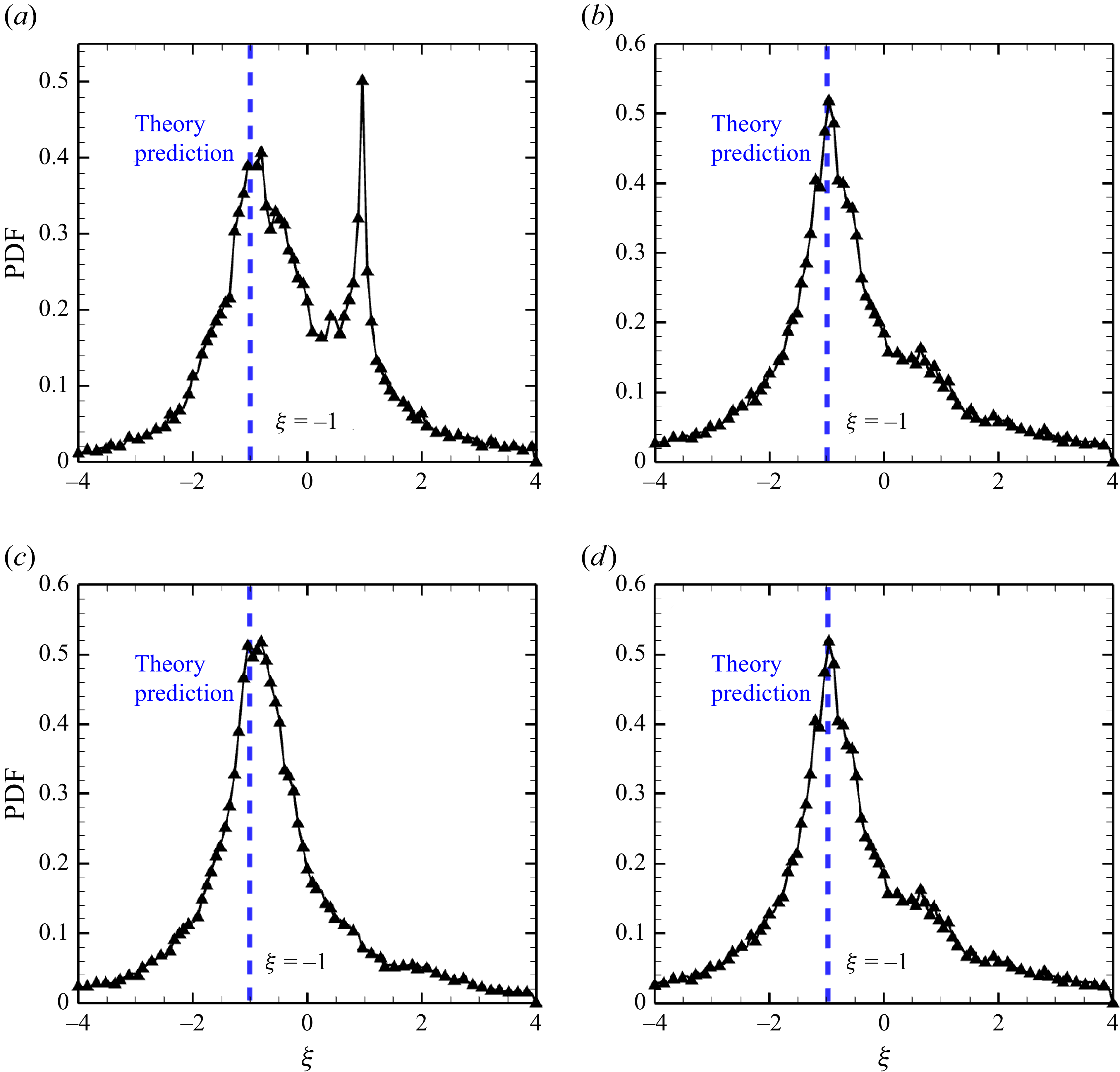
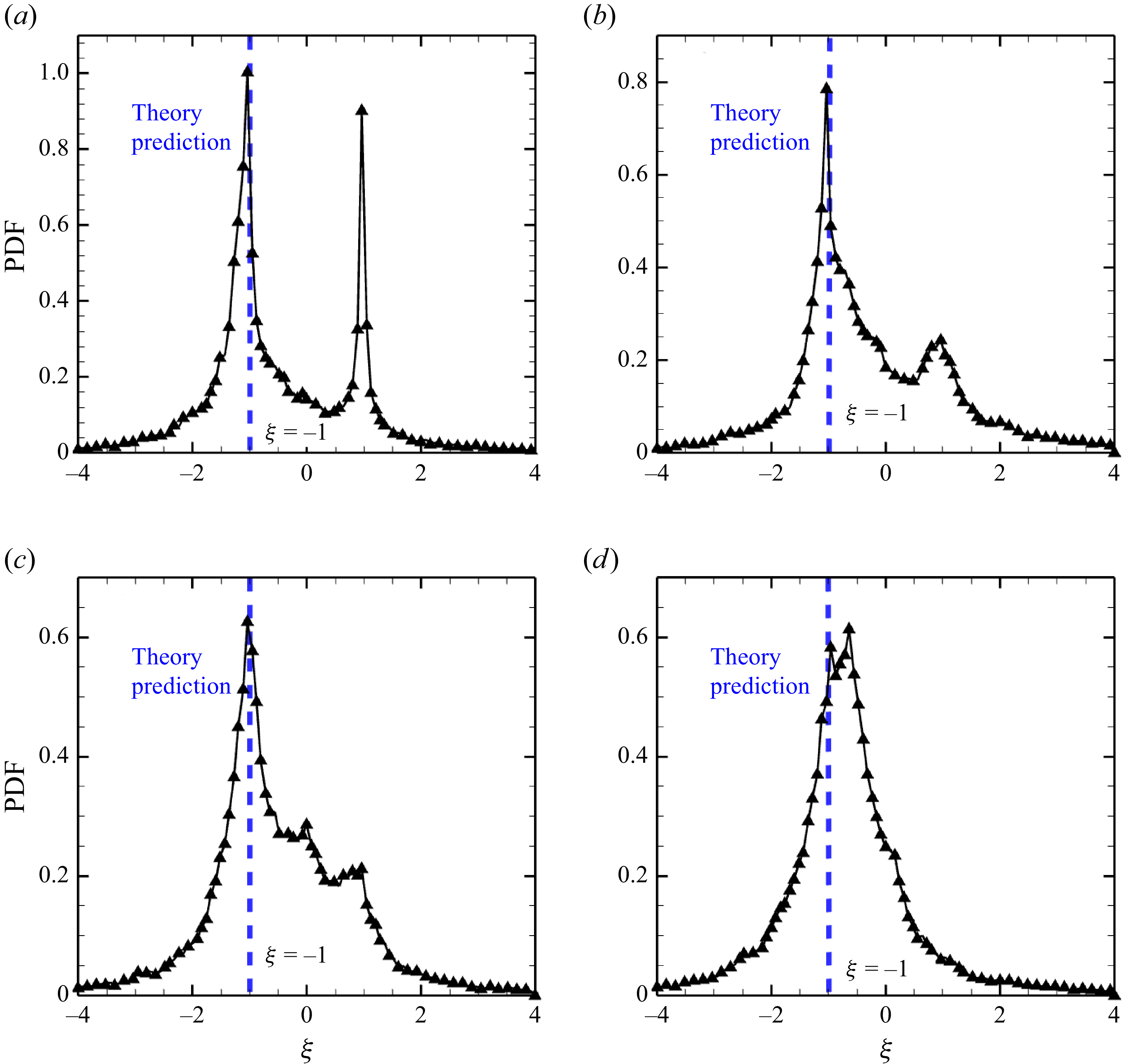
where $\xi = (\widetilde{W_{12}}+\omega/2)(1/2(s_1-s_2))$ is the essential parameter that determines the stability of this equation (Lapeyre et al. Reference Lapeyre, Klein and Hua1999). With the analytical expressions for the principal strain rate $s_i$ and the related parameters given in (3.13), $\xi$ satisfies the relationship

(3.18) \begin{equation} \xi = \frac{\widetilde {W_{12}} + \omega /2}{\dfrac {1}{2}\left (s_1-s_2\right )} = -1. \end{equation}

By transforming the angle $\theta$ and time $t$ with the following relationships:

(3.19) \begin{equation} \left \{ \begin{aligned} & \zeta = -2\theta + \frac{\pi }{2},\\ & \tau = \int _{0}^{t}2s_1\left (t'\right ){\textrm {d}}t', \end{aligned} \right . \end{equation}

then (3.17) can be can be reformulated into a simple ordinary differential equation (ODE)

(3.20) \begin{equation} \frac{\textrm {d}}{{\textrm {d}}\tau }\zeta = 1 - \cos \zeta . \end{equation}

The solution to this ODE is

(3.21) \begin{equation} \zeta = \pi + 2\arctan \left (\tau \right )\!. \end{equation}

Thus, the analytical solution for the alignment of the scalar gradient $\lambda _i$ in (3.10) is given by

(3.22) \begin{equation} \lambda _1 = \cos \left (-\frac{\pi }{4} + \arctan \left (\tau \right )\right )\!,\qquad \lambda _2 = \sin \left (-\frac{\pi }{4} + \arctan \left (\tau \right )\right )\!. \end{equation}

Figure 8.

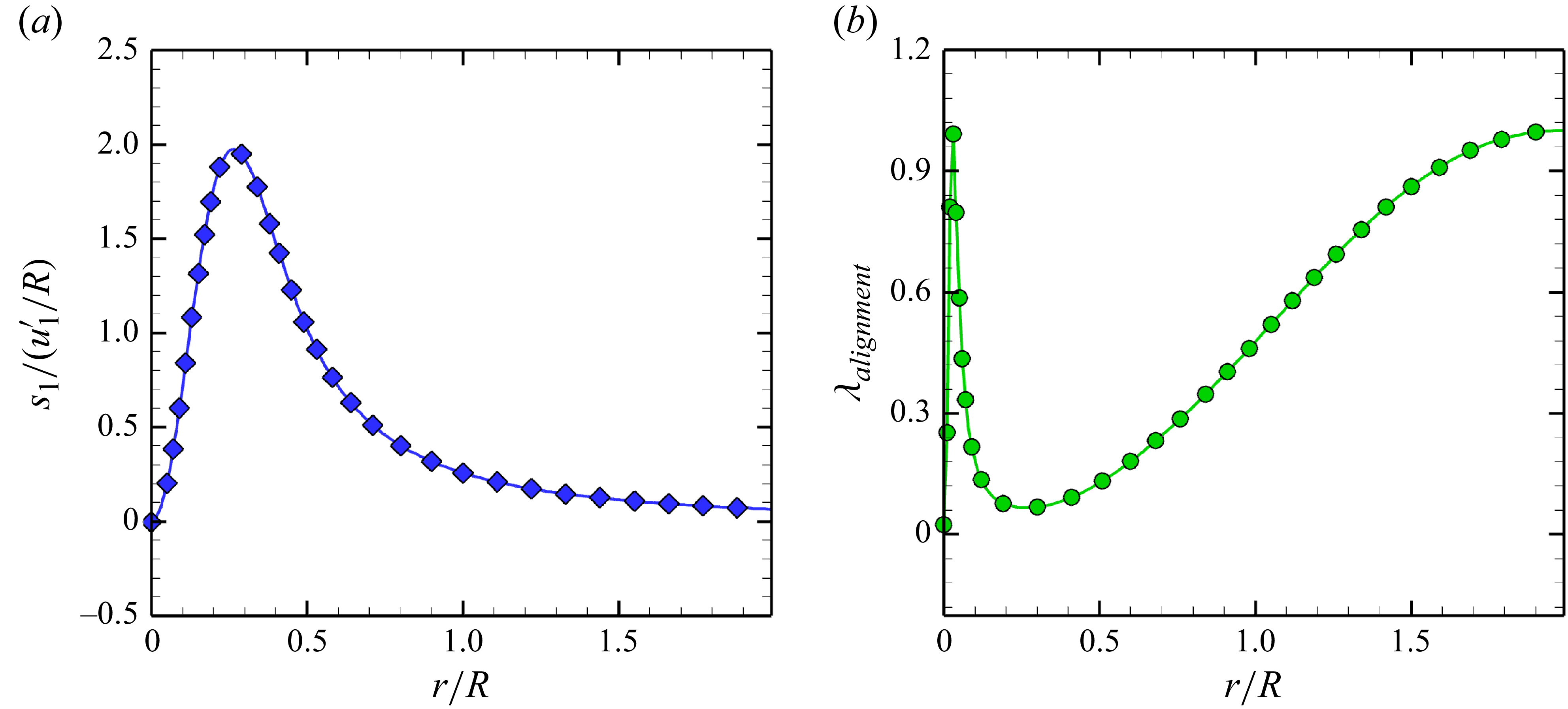
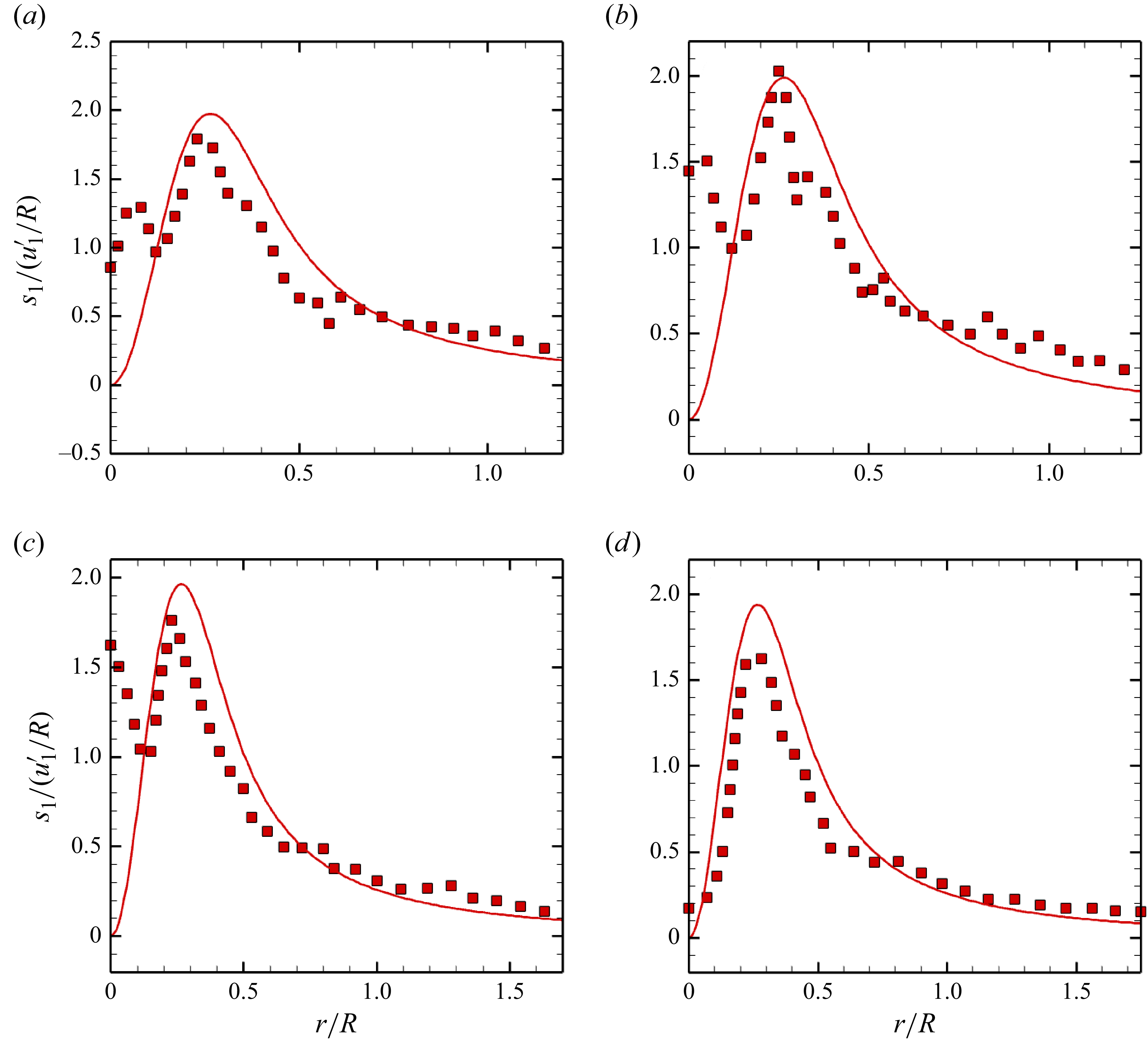
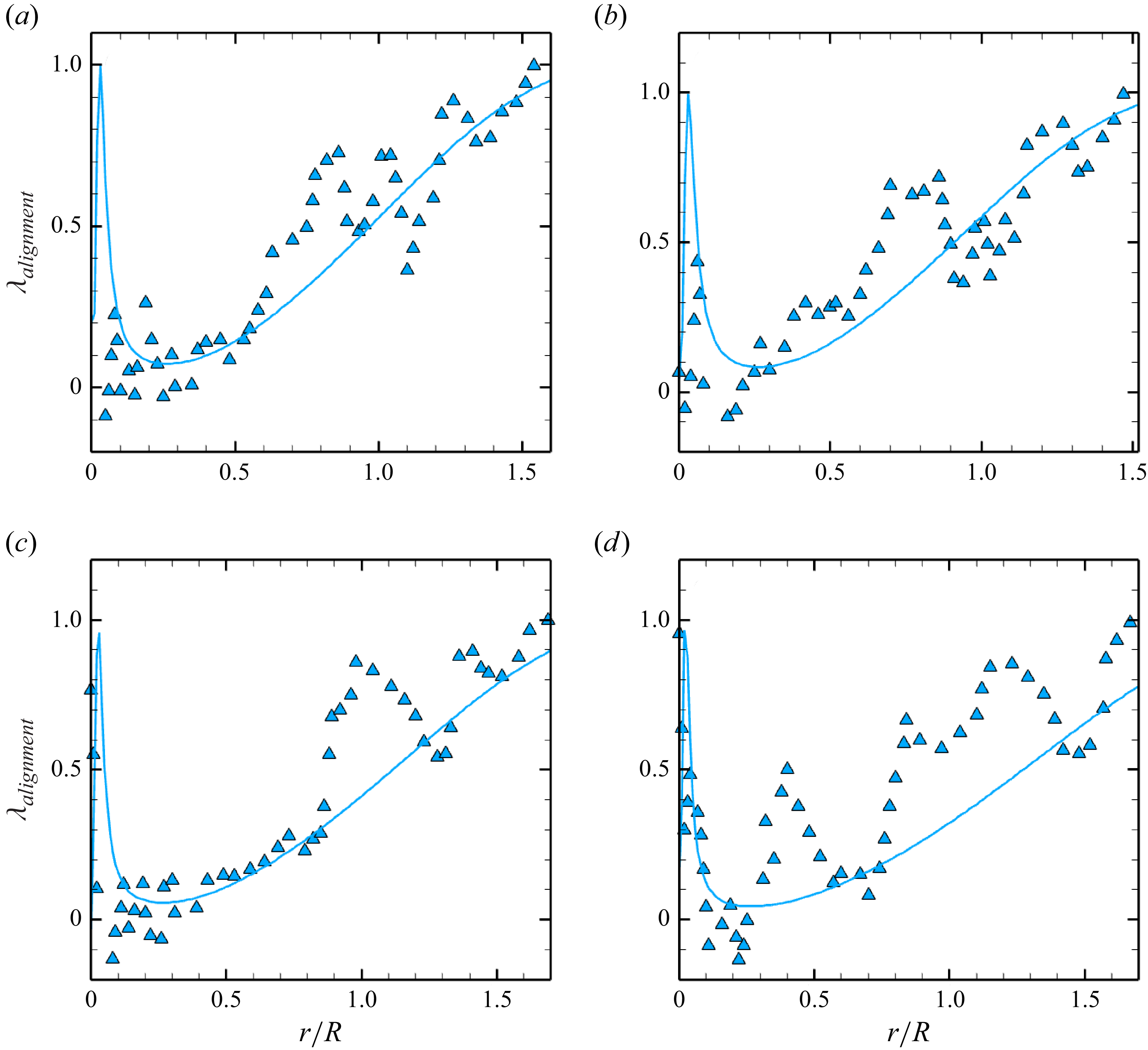
The examples for the distribution of $(a)$ the principal strain rate and $(b)$ the comprehensive alignment effect $\lambda _{\textit{alignment}}$ along the radial axis in a single vortex as in (3.23). Here, the principal strain rate is normalised by the ratio between the post-shock air velocity $u_1^{\prime}$ and the radius of the helium bubble $R$ .

With the analytical solution of the SDGEs for the principal strain rate in (3.7) and the alignment of the scalar gradient in (3.10), the stretching rate, as defined in (1.5), can be determined within a single vortex as follows:

(3.23) \begin{equation} R_{\textit{stretch}} = 2s_1\lambda _{\textit{alignment}} = 4s_1\frac{\tau }{1+\tau ^2}, \end{equation}

where

(3.24) \begin{equation} \lambda _{\textit{alignment}} = 1-2\lambda _1^2 = 2\frac{\tau }{1+\tau ^2}. \end{equation}

In this expression, $\lambda _{\textit{alignment}}$ indicates the comprehensive effect of the scalar gradient alignment on the stretching rate. Examples for the distribution of the principal strain $s_1$ and the comprehensive alignment effect $\lambda _{\textit{alignment}}$ along the radial axis under the condition of PS SBI are illustrated in figure 8. Notably, if the diffusion term in (3.6) is neglected, the analytical expression for the stretching rate in (3.23) corresponds to the algebraic growth of SDR $\chi$

(3.25) \begin{equation} \frac{\textrm {d}}{{\textrm {d}}t}\chi = T_{\textit{stretch}}^{\chi } = \chi R_{\textit{stretch}} \quad \Rightarrow \quad \chi = \chi _0\left (1+\tau ^2\right )\!. \end{equation}

This algebraic stretching characteristic will be further elaborated on from a geometric perspective in the subsequent discussion.

3.4. Physical meaning of the algebraic stretching rate: from the geometric view point

This subsection elucidates the physical meaning of the analytical expression for the stretching rate $R_{stetch}$ presented in (3.23) from the geometric viewpoint. Referring back to the governing equation for the SDR in (3.6), the stretching term $T_{\textit{stretch}}^{\chi }$ , from which the definition of the stretching rate $R_{\textit{stretch}}$ is derived, describes the evolution of the scalar gradient magnitude $\boldsymbol{\nabla }Y$ during a continuous stretching process without molecular diffusion. Figure 9 is the schematic illustrating the impact of the stretching rate $R_{\textit{stretch}}$ on SDR within a single vortex.

Figure 9.

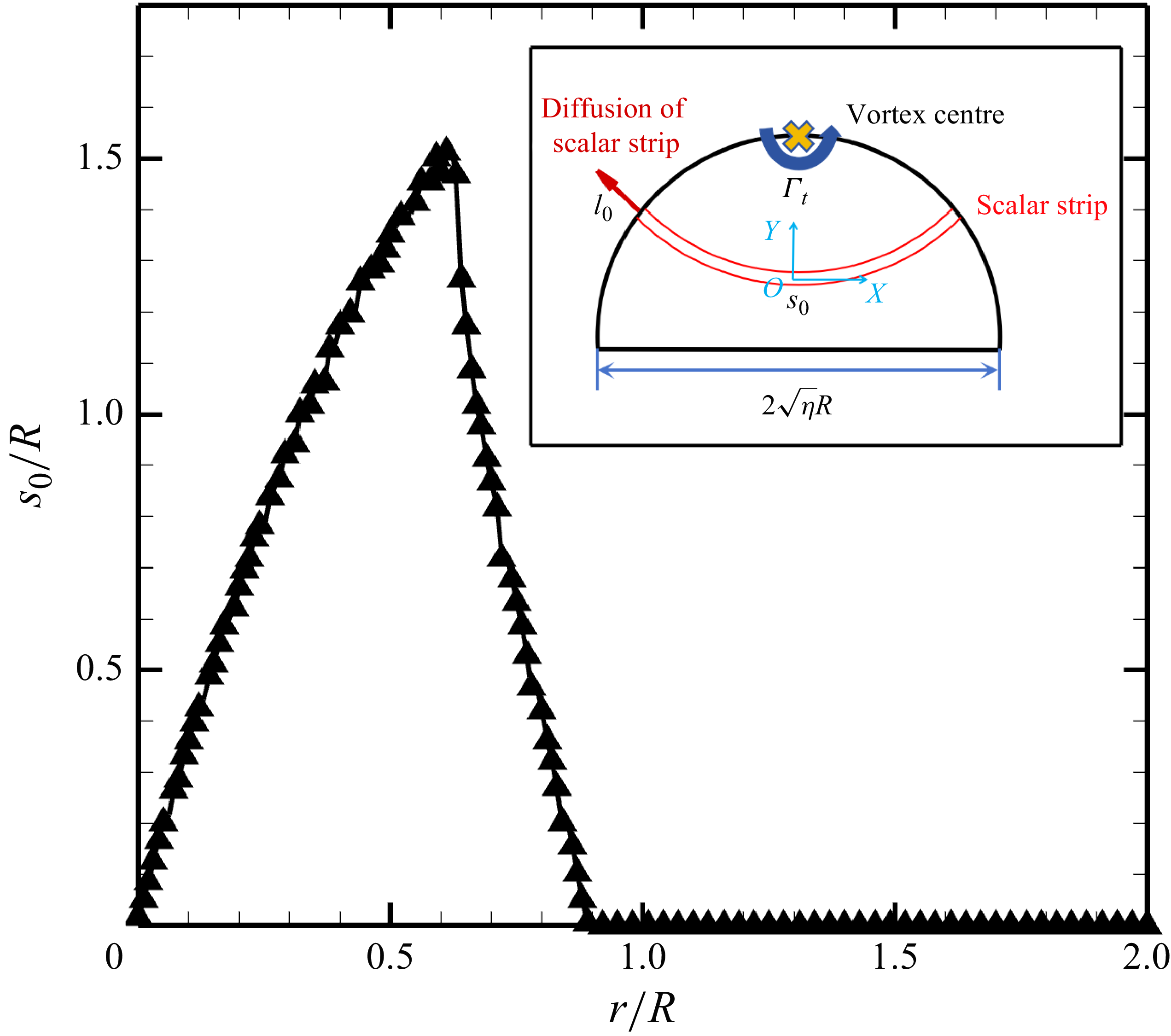
Schematic illustration of the impact of the stretching rate $R_{\textit{stretch}}$ on SDR growth in a single vortex. Within this diagram, the area outlined by the red dashed line represents the initial scalar strip, while the area enclosed by the red solid line denotes the deformed scalar strip as influenced by the stretching effect of the single vortex. The line perpendicular to the scalar gradient represents the scalar strip length $l(t)$ , while the parallel line represents the scalar strip width $s(t)$ . According to the estimation for SDR $\chi \sim |\Delta Y|^2/s(t)^2$ , the influence of the stretching rate on SDR growth is reflected in the continuous decrease in the scalar strip width $s(t)$ .

As shown in figure 9, the initial scalar strip, with a length of $l_0$ and a width of $s_0$ , undergoes deformation due to the continuous stretching effect of the single vortex. This stretching effect elongates the scalar strip to a new length $l(t)$ , while compressing its width to $s(t)$ in accordance with the conservation of the scalar strip’s area. The definition of the SDR, $\chi = \lvert \boldsymbol{\nabla }Y\rvert \lvert \boldsymbol{\nabla }Y\rvert$ , suggests that the essence of SDR is the square of the magnitude of the scalar gradient. Considering that the SDR for the scalar strip can be approximated by the ratio of the mass fraction difference $\Delta Y$ to the width $s(t)$ , expressed as $\chi \sim \lvert \Delta Y \rvert ^2/s(t)^2$ , an increase in SDR appears to stem from the reduction in the width of the deformed scalar strip $s(t)$ with a constant mass fraction difference $\Delta Y$ when the diffusion process is neglected. This observation indicates how the stretching term $T_{\textit{stretch}}^{\chi }$ drives the growth of SDR.

Under this schematic, the stretching of SDR can be transformed to the reduction in the width of the scalar strip. If the diffusion term $T_{\textit{diff}}^{\chi }$ is neglected, the governing equation for SDR in (3.6) can be rewritten based on the estimation $\chi \sim 1/s(t)^2$

(3.26) \begin{equation} \frac{\textrm {d}}{{\textrm {d}}t}\chi = T_{\textit{stretch}}^{\chi } = \chi R_{\textit{stretch}} \quad \Rightarrow \quad \frac{\textrm {d}}{{\textrm {d}}t}\left (\frac{1}{s(t)}\right )^2 = \left (\frac{1}{s(t)}\right )^2 R_{\textit{stretch}}. \end{equation}

Applying the analytical expression of the stretching rate $R_{\textit{stretch}}$ in (3.23), this equation becomes

(3.27) \begin{equation} \frac{\textrm {d}}{{\textrm {d}}t}\left (\frac{1}{s(t)}\right )^2 = \left (\frac{1}{s(t)}\right )^2 4s_1\frac{\tau }{1+\tau ^2}, \end{equation}

with the analytical solution

(3.28) \begin{equation} s\left (t\right ) = \frac{s_0}{\sqrt {1+\tau ^2}}, \end{equation}

and the corresponding evolution of the elongation in the length of the scalar strip $l(t)$ is demonstrated by

(3.29) \begin{equation} l(t) = l_0\sqrt {1+\tau ^2}. \end{equation}

Figure 10.

The schematic illustrating the validation of the algebraic stretching characteristic in a single vortex using the Lagrangian method. Referring to the previous investigation (Liu et al. Reference Liu, Yu, Zhang and Xiang2022), the stretching of a post-shock bubble is approximated as a compressed semicircle composed of a series of scalar strips, each undergoing deformation due to the continuous stretching effect of the single vortex. $(a)$ The distribution of initial scalar strips used to approximate the stretching process of the post-shock bubble. (b) An example of a stretched scalar strip, along with the corresponding strain eigenframe $(\boldsymbol{e}_1,\boldsymbol{e}_2)$ and the scalar gradient. $(c)$ The results of the Lagrangian particle movement for the scalar strip depicted in $(a)$ .

These solutions reveal that the length $l(t)$ and the width $s(t)$ evolve in an algebraic form over time, indicating that the stretching within a single vortex displays an algebraic stretching characteristic.

Figure 11.

The comparison of the length of the scalar strip at different radii obtained from the Lagrangian particle movement results and prediction of the stretching dynamics derivation in (3.29).

Based on the derivation of the stretching behaviour of the scalar strip, the algebraic stretching characteristic is further validated using the Lagrangian method (Liang et al. Reference Liang, Yu, Zhang, Xu and Liu2019; Zhang et al. Reference Zhang, Liu, Yu, Wang, He and Liu2022). The morphological changes of the bubble following shock interaction, as shown in figure 4, support assumption PS.(iv), which approximates the mixing of the post-shock bubble as the mixing of a compressed semicircle composed of a series of scalar strips, as illustrated in figure 10 $(a)$ . This approximation aligns with our previous investigation (Liu et al. Reference Liu, Yu, Zhang and Xiang2022). For one of the initial scalar strips with a length $l_0$ , perpendicular to the scalar gradient, and a width $s_0$ , parallel to the scalar gradient, the Lagrangian particle movement results in figure 10 $(c)$ demonstrate the continuous elongation of the length $l(t)$ and reduction of the width $s(t)$ . By comparing the lengths of the scalar strips at different radii, obtained according to the trajectories of the Lagrangian particles placed at the edge of semicircle, as shown in figure 10 $(b)$ , with the predictions of the stretching dynamics derivation in (3.29), figure 11 demonstrates the good agreement between the Lagrangian particle movement results and theoretical predictions, thereby the algebraic stretching characteristic within a single vortex is confirmed.

4.1. Verification of algebraic stretching in PS SBI

After the shock interaction, the PS bubble attains a translational velocity $V_v$ that is approximately equal to the post-shock velocity $u_1^{\prime}$ . By setting the origin of the cylindrical coordinates at the centre of the moving vortex (Shariff & Leonard Reference Shariff and Leonard1992), the azimuthal velocity around the vortex can be expressed as $(u {-} V_{v},v)$ , where $u$ represents the velocity in the $x$ -direction and $v$ denotes the velocity in the $y$ -direction. In figure 12, mixing in PS SBI is passively governed by the large-scale main vortex. Given the reduction of the density difference, it is reasonable to assert that the stretching dynamics in PS SBI aligns with the single-vortex algebraic stretching discussed in § 3. This assumption is further validated by analysing the azimuthally averaged parameters along the radius

(4.1) \begin{equation} f\left (r,\left .\varphi \right |_{avg}\right )=\frac{\int _{Y\gt 0.01Y_{\textit{max}}}f(r,\varphi ){\textrm {d}}\varphi }{\int _{Y\gt 0.01Y_{\textit{max}}}{\textrm { d}}\varphi }, \end{equation}

as illustrated by the blue circle in figure 12 $(b)$ .

Figure 12.

The distribution of the normalised mass fraction $Y/Y_{\textit{max}}$ and the relative azimuthal velocity around the vortex centre $(u-V_{v},v)$ in PS SBI at $(a)$ $t = 13.2\ \unicode{x03BC} {\textrm {s}}$ , $(b)$ $t = 26.4\ \unicode{x03BC} {\textrm {s}}$ , $(b)$ $t = 39.6\ \unicode{x03BC} {\textrm {s}}$ , $(d)$ $t = 52.8\ \unicode{x03BC} {\textrm {s}}$ . The red dash-dot dot line represents the isoline where $Y=0.01Y_{\textit{max}}$ .

Based on the single-vortex stretching dynamics described in (3.23), we first examine the principal strain rate in PS SBI. Figure 13 illustrates the distribution of the azimuthally averaged principal strain rate $s_1$ along the radial axis in PS SBI. With the total circulation of $\varGamma _{t} \approx 2.1\ {\textrm {m}^2\,\rm s^{-1}}$ , the analytical expression for the principal strain rate can be expressed as follows:

(4.2) \begin{equation} s_{1} = \frac{\varGamma _{t}}{2\pi r^2}\left (1 - \exp \left (-\frac{r^2}{4\nu (t + t_0)}\right )\right ) - \frac{\varGamma _{t}}{8\pi \nu (t+t_0)}\exp \left (-\frac{r^2}{4\nu (t + t_0)}\right )\!, \end{equation}

where $t_0$ is estimated based on the scale of the vortex core (Saffman Reference Saffman1970)

(4.3) \begin{equation} \sqrt {4\nu t_0} = r(s_1^{\textit{max}}) \approx 0.27 R, \quad \Rightarrow \quad t_{0} \approx 9.8\times 10^{-4} {\textrm {s}}. \end{equation}

Notably, since $t_0 \gg t$ , the principal strain rate evolves as a nearly steady state, which corresponds with the observation of the nearly steady single vortex depicted in figure 12. The comparison shown in figure 13 demonstrates that the principal strain rate in PS SBI aligns closely with the theoretical distribution outlined in (4.2). This correspondence indicates that the stretching dynamics in PS SBI exhibits a characteristic consistent with single-vortex stretching from the first perspective of the principal strain rate.

Figure 13.

The distribution of the azimuthally averaged principal strain rate $s_1$ on the radial axis in PS SBI. The moments captured from $(a)$ to $(d)$ are the same as those of figure 12. The azimuthally averaged principal strain rate is plotted as the red dots, while the prediction of the theory in (4.2) is plotted as the red solid line.

Another important parameter for stretching dynamics is the alignment of the scalar gradient $\lambda _{\textit{alignment}}$ . Referring to the derivation of the SDGE- $\lambda _i$ in (3.10), a significant result for the parameter $\xi ={(\widetilde{W_{12}}}+\omega/2)/{((s_1-s_2)/2)}$ , which determines the stability of SDGE- $\lambda _i$ , is that $\xi$ satisfies the relationship $\xi = -1$ within a single vortex (3.18).

Figure 14.

The probability density function (PDF) of the parameter $\xi = ({\widetilde {W_{12}} + \omega /2})/({({1}/{2})(s_1-s_2)})$ in PS SBI at the same moments as those of figure 12.

The probability density function (PDF) of $\xi$ in PS SBI is obtained from the region enclosed by the red dash-dot-dot line in figure 12, with the corresponding results shown in figure 14. Notably, the PDF curves exhibit pronounced peaks centred around $\xi = -1$ . The deviations from the theoretical value of $\xi = -1$ , such as the emergence of $\xi =1$ in the early stages, can be attributed to the small discrepancies between PS SBI and an idealised single vortex. To evaluate whether the relationship given in (3.18) remains applicable in PS SBI, we examine if the solution of SDGE- $\lambda _i$ as derived in § 3 based on (3.18), accurately describes the alignment of the scalar gradient $\lambda _{\textit{alignment}}$ . If (3.18) holds, the distribution of $\lambda _{\textit{alignment}}$ should follow the theoretical prediction given in (3.24): $\lambda _{\textit{alignment}} = 2\tau /(1+\tau ^2)$ , where $\tau$ is defined as $\tau = \int _{0}^{t}2s_1(t'){\textrm {d}}t'$ , and the expression for $s_1$ is consistent with that provided in (4.2).

Figure 15.

The distribution of the azimuthally averaged alignment of the scalar gradient $\lambda _{\textit{alignment}}$ on the radial axis in PS SBI. The moments captured from $(a)$ to $(d)$ are the same as those of figure 12. The azimuthally averaged alignment is plotted as the blue dots, while the prediction of the theory in (3.24) is plotted as the blue solid line.

Figure 15 presents a comparison between the azimuthally averaged $\lambda _{\textit{alignment}}$ in PS SBI and the theoretical prediction provided in (3.24). The distribution of $\lambda _{\textit{alignment}}$ is accurately captured by the theory described in (3.24). The minor discrepancies observed are likely due to the intrinsic complexity of alignment dynamics described by SDGE- $\lambda _i$ in (3.10), which incorporates the coupled effects of pressure and velocity gradients. These results support the validity of (3.18) in PS SBI, suggesting that the stretching dynamics within this flow exhibits characteristic consistent with single-vortex stretching from the second perspective of scalar gradient alignment.

4.2. Incorporating diffusion process based on algebraic stretching rate

The stretching dynamics in PS SBI has been shown to exhibit the characteristic of single-vortex stretching from two perspectives: the principal strain rate $s_1$ and the alignment of the scalar gradient $\lambda _{\textit{alignment}}$ . However, as indicated in the analysis of the decomposition of the material derivative of the total SDR ${{\textrm {D}}\langle \chi \rangle }/{{\textrm {D}}t}$ presented in figure 7, the diffusion term $\langle T_{\textit{diff}}^{\chi } \rangle$ in (3.6) serves as another significant factor influencing the evolution of the SDR. Therefore, incorporating the diffusion process based on the algebraic stretching rate is essential for developing the PS mixing model for SDR $\langle \chi \rangle$ .

As presented in figure 9, the estimation $\chi \sim \lvert \Delta Y \rvert ^2/s(t)^2$ suggests that the diffusion effect reduces the SDR $\chi$ by altering the magnitude of the mass fraction difference $\lvert \Delta Y \rvert$ . To model this diffusion effect within a post-shock cylindrical bubble, it is convenient to apply assumption PS.(iv) to assume that the mixing occurs on a compressed semicircle illustrated in figure 10. The radius of this semicircle is $\sqrt {\eta }R$ , where $\eta \approx 0.42$ represents the compression rate of PS SBI. By transforming the advection–diffusion equation (2.14) into the coordinate system $(O,X,Y)$ shown in figure 16, the equation can be reformulated as

(4.4) \begin{equation} \frac{\partial Y}{\partial t} + U\frac{\partial Y}{\partial x} + V\frac{\partial Y}{\partial y} = \mathcal{D}\left (\frac{\partial ^2 Y}{\partial x^2} + \frac{\partial ^2 Y}{\partial y^2}\right )\!, \end{equation}

where the origin of the $(O,X,Y)$ system is a Lagrangian frame set on a moving scalar strip. The direction of this frame changes over time in response to the stretching motion.

Figure 16.

The schematic of the moving coordinate $(O,X,Y)$ on the deformed scalar strips and the distribution of the related width $s_0$ of the initial scalar strips in the compressed semicircle depicted in figure 10.

On this moving coordinate, the relative velocity $(U,V)$ can be expressed in terms of the deformation rate of the scalar strip, as described by (Villermaux Reference Villermaux2019)

(4.5) \begin{equation} \left \{ \begin{aligned} & U = \frac{{\textrm {d}}x}{{\textrm {d}}t} = \frac{{\textrm {d}}x}{{\textrm {d}}s(t)}\frac{{\textrm {d}}s(t)}{{\textrm {d}}t} = \frac{x}{s(t)}\frac{{\textrm {d}}s}{{\textrm {d}}t},\\ & V = \frac{{\textrm {d}}y}{{\textrm {d}}t} = \frac{{\textrm {d}}y}{{\textrm {d}}s(t)}\frac{{\textrm {d}}s(t)}{{\textrm {d}}t} = -\frac{y}{s(t)}\frac{{\textrm {d}}s(t)}{{\textrm {d}}t}, \end{aligned} \right . \end{equation}

where $s(t)$ denotes the instantaneous width of the scalar strip. Considering the mass fraction gradient $\boldsymbol{\nabla }Y$ is predominantly aligned with the X-direction, i.e. $\lvert {\partial Y}/{\partial x} \rvert \gg \lvert {\partial Y}/{\partial y}\rvert$ , (4.4) becomes

(4.6) \begin{equation} \frac{\partial Y}{\partial t} + \frac{x}{s(t)}\frac{{\textrm {d}}s(t)}{{\textrm {d}}t}\frac{\partial Y}{\partial x} = \mathcal{D}\frac{\partial ^2 Y}{\partial x^2}. \end{equation}

Since the stretching dynamics is PS SBI is proved to exhibit the single-vortex stretching characteristic, the width $s(t)$ evolves algebraically as in (3.28). Using the canonical transformation introduced by Ranz (Reference Ranz1979)

(4.7) \begin{equation} \left \{ \begin{aligned} & \varsigma = \frac{x}{s(t)},\\ & \tau ^{\mathcal{D}} = \int _{0}^{t}\frac{\mathcal{D}{\textrm {d}}t'}{s(t')^2} , \end{aligned} \right . \end{equation}

then (4.6) is transformed into a simple Fourier equation

(4.8) \begin{equation} \frac{\partial Y}{\partial \tau ^{\mathcal{D}}} = \frac{\partial ^2 Y}{\partial \varsigma ^2}, \end{equation}

with the initial condition specified as

(4.9) \begin{equation} Y(\tau ^{\mathcal{D}} = 0) = \left \{ \begin{aligned} & 1 \quad \lvert \varsigma \rvert \leqslant \frac{1}{2},\\ & 0 \quad \lvert \varsigma \rvert \gt \frac{1}{2}. \end{aligned} \right . \end{equation}

Figure 17.

Comparison of the evolution of total SDR $\langle \chi \rangle$ in PS SBI with theoretical predictions: the red solid line represents the prediction from the PS mixing model in (4.11), and the black dashed line denotes the two-stage approximation from (4.15) and (4.16), which aligns with the approximation of SDR by Meunier & Villermaux (Reference Meunier and Villermaux2003). The blue line indicates the PS mixing time $t_{m}^{\textit{ps}}$ obtained from the previous research (Liu et al. Reference Liu, Yu, Zhang and Xiang2022).

Subsequently, the mass fraction in the moving coordinate frame will diffuse and spread according to the following solution:

(4.10) \begin{equation} Y\left (\varsigma ,\tau ^{\mathcal{D}}\right ) = \frac{1}{2}\left [{\textrm {erf}}\left (\frac{\varsigma + 1/2}{2\sqrt {\tau ^{\mathcal{D}}}}\right ) - {\textrm {erf}}\left (\frac{\varsigma - 1/2}{2\sqrt {\tau ^{\mathcal{D}}}}\right ) \right ]. \end{equation}

By considering the mass fraction difference $\Delta Y$ alongside the mass fraction distribution from (4.10), the PS mixing model for the total SDR $\langle \chi \rangle$ can be proposed as

(4.11) \begin{equation} \left \langle \chi \right \rangle = \int \left (\int _{-\infty }^{+\infty }\left (\frac{{\textrm {d}}Y}{{\textrm {d}}x}\right )^2{\textrm {d}}x\right ) {\textrm {d}}y = \int _{0}^{\sqrt {2\eta }R}\frac{1+\tau ^2}{s_0}\frac{1}{\sqrt {2\pi \tau ^{\mathcal{D}}}}\left (1-\mathrm{e}^{-\frac{1}{8\tau ^{\mathcal{D}}}}\right ) {\textrm {d}}r. \end{equation}

In this model, $\tau = \int _{0}^{t}2s_1(t'){\textrm {d}}t'$ represents the transformed time corresponding to the stretching dynamics, while $\tau ^{\mathcal{D}} = \int _{0}^{t} {\mathcal{D}{\textrm {d}}t'}/{s(t')^2} = \int _{0}^{t} {\mathcal{D} (1+\tau ^2 ){\textrm {d}}t'}/{s_0^2}$ indicates the transformed time according to the diffusion process.

The comparison shown in figure 17 indicates that the PS mixing model presented in (4.11) accurately predicts the evolution of the total SDR $\langle \chi \rangle$ during mixing in PS SBI, which proves that the mixing in PS SBI is predominantly governed by the algebraic stretching rate within a single vortex. Furthermore, we can notice the presence of the characteristic time $t_{\textit{charac}}$ , which delineates the mixing process into two distinct stages: when $t \lt t_{\textit{charac}}$ , the total SDR $\langle \chi \rangle$ increases to its peak value; subsequently, for $t \geqslant t_{\textit{charac}}$ , it transitions into the decay stage. The existence of this characteristic time and the two distinct mixing stages can be explained through two-stage approximation of (4.11).

In relation to the transformed time associated with the stretching dynamics, defined as $\tau = \int _{0}^{t}2s_1(t'){\textrm {d}}t'$ , and given the nearly steady principal strain rate $s_1$ illustrated in figure 4.2, $\tau$ can be approximated as

(4.12) \begin{equation} \tau \approx 2s_1 t. \end{equation}

Consequently, the width of the scalar strips evolves according to

(4.13) \begin{equation} s(t) = \frac{s_0}{\sqrt {1+\tau ^2}} =\frac{s_0}{\sqrt {1+4s_1^2t^2}}, \end{equation}

which simplifies the expression for the transformed time related to diffusion $\tau ^{\mathcal{D}}$ as follows:

(4.14) \begin{equation} \tau ^{\mathcal{D}} = \int _{0}^{t}\frac{\mathcal{D}{\textrm {d}}t'}{s(t')^2} = \frac{\mathcal{D}}{s_0^2}\left (t + \frac{4}{3}s_1^2t^3\right ) \approx \frac{4}{3}\frac{\mathcal{D}}{s_0^2}s_1^2t^3. \end{equation}

In the context of (4.11), if $\tau ^{\mathcal{D}} \lt {1}/{8}$ , i.e. $t \lt t_{\textit{charac}}=((3/32)(s_0^2/(s_1^2\mathcal{D})))^{(1/3)}$ , (4.11) can be modified to

(4.15) \begin{equation} \begin{aligned} \left \langle \chi \right \rangle & = \int _{0}^{\sqrt {2\eta }R}\frac{1+\tau ^2}{s_0}\frac{1}{\sqrt {2\pi \tau ^{\mathcal{D}}}}\left (1-\mathrm{e}^{-\frac{1}{8\tau ^{\mathcal{D}}}}\right ) {\textrm {d}}r \\ & \approx \int _{0}^{\sqrt {2\eta }R}\frac{1+\tau ^2}{s_0}\frac{1}{\sqrt {2\pi \tau ^{\mathcal{D}}}}{\textrm {d}}r \approx \int _{0}^{\sqrt {2\eta }R}\sqrt {\frac{6}{\pi \mathcal{D}}}s_1t^{\frac{1}{2}}{\textrm {d}}r, \end{aligned} \end{equation}

indicating the growth stage of $\langle \chi \rangle$ . During this phase, the growth of $\langle \chi \rangle$ arises from the dominance of the stretching effect $ ({1+\tau ^2})/{s_0}$ in the PS mixing process. Conversely, if $\tau ^{\mathcal{D}} \geqslant {1}/{8}$ , i.e. $t \geqslant t_{\textit{charac}} =((3/32)(s_0^2/(s_1^2\mathcal{D})))^{(1/3)}$ , the equation transforms to

(4.16) \begin{equation} \begin{aligned} \left \langle \chi \right \rangle & = \int _{0}^{\sqrt {2\eta }R}\frac{1+\tau ^2}{s_0}\frac{1}{\sqrt {2\pi \tau ^{\mathcal{D}}}}\left (1-\mathrm{e}^{-\frac{1}{8\tau ^{\mathcal{D}}}}\right ) {\textrm {d}}r \\ & \approx \int _{0}^{\sqrt {2\eta }R}\frac{1+\tau ^2}{s_0}\frac{1}{\sqrt {2\pi \tau ^{\mathcal{D}}}}\frac{1}{8\tau ^{\mathcal{D}}} {\textrm {d}}r\approx \int _{0}^{\sqrt {2\eta }R}\frac{3}{16}\sqrt {\frac{3}{2\pi }}\frac{s_0^2}{\mathcal{D}^{\frac{3}{2}}s_1 t^{\frac{5}{2}}}{\textrm {d}}r, \end{aligned} \end{equation}

which characterises the decay stage of $\langle \chi \rangle$ . In this phase, the decay of $\langle \chi \rangle$ stems from the predominance of the diffusion effect $ {1}/{\sqrt {2\pi \tau ^{\mathcal{D}}}} (1-\mathrm{e}^{-{1}/{8\tau ^{\mathcal{D}}}} )$ in the PS mixing process. The rationale of these equation simplifications is provided in the supplementary material. Notably, the two-stage approximations of the PS mixing model are consistent with the approximations for $\langle \chi \rangle$ in the previous study on single-vortex PS mixing (Meunier & Villermaux Reference Meunier and Villermaux2003). As shown in figure 17, the two-stage approximation of the PS mixing model in (4.15) and (4.16) accurately captures the trends of SDR evolution during both the growth and decay stages, while still overestimating the evolution of SDR. Compared with this previous estimation of SDR, the PS mixing model effectively synthesises the stretching dynamics and diffusion effects in (3.6), providing a robust predictive framework for the evolution of $\langle \chi \rangle$ . Furthermore, compared with the mixing time for PS SBI predicted by the mixing time model in our earlier work (Liu et al. Reference Liu, Yu, Zhang and Xiang2022), indicated by the blue line in figure 17, the PS mixing model offers a more detailed description of the evolution of mixing indicator, representing a significant advancement over the theory for mixing time prediction.

5.1. Secondary baroclinic effect on stretching dynamics in VD SBI

This section examines whether the stretching dynamics in VD SBI manifests the same single-vortex stretching characteristic as observed in PS SBI. Specifically, the azimuthally averaged principal strain rate $s_1$ in VD SBI is compared with the predictions of single-vortex stretching model as outlined in (4.2). As illustrated in figure 19, the current single-vortex stretching model underestimates $s_1$ in VD SBI. In deriving the distribution of $s_1$ for the single vortex, the application of assumption PS.(iii) neglected the density gradient $\boldsymbol{\nabla }\rho$ , leading to an oversimplified SDGE- $s_i$ in (3.12), where only viscous effect is considered. Therefore, the inclusion of the baroclinic term, $(-{1}/{2\rho}) ({1}/{r})({\partial \rho }/{\partial \varphi })({\partial p}/{\partial r})$ , as outlined in (3.11), should be reconsidered in the analysis of VD SBI to provide a more accurate depiction of the principal strain rate $s_1$ . Notably, the governing equation for $s_1$ shares the same mathematical structure as that for vorticity $\omega$ . Thus, the influence of the baroclinic term can be reflected by SBV, a canonical phenomenon in VD mixing, as reported in several studies (Peng et al. Reference Peng, Yang, Wu and Xiao2021a , Reference Peng, Yang and Xiaob ; Liu et al. Reference Liu, Yu, Zhang and Xiang2022). As shown in figure 20, SBV manifests as a vortex-bilayer structure characterised by dominant negative vorticity and intensified positive vorticity. This structure is quantitatively described using the positive and negative circulation, defined as follows, consistent with prior investigations (Peng et al. Reference Peng, Zabusky and Zhang2003; Niederhaus et al. Reference Niederhaus, Greenough, Oakley, Ranjan, Anderson and Bonazza2008):

(5.1) \begin{equation} \left \{ \begin{aligned} &\varGamma ^{+} = \iint _{\omega \gt 0} \omega {\textrm {dV}}, \\ &\varGamma ^{-} = \iint _{\omega \lt 0} \omega {\textrm {dV}}. \end{aligned} \right . \end{equation}

Figure 20 $(b)$ describes the evolution of positive and negative circulations: prior to the time $t_{sbv} \approx 7.2 \rm {\ \unicode {x03BC} s}$ , the shock interaction with the bubble triggers the formation of the primary vortex. After $t \gt t_{sbv}$ , the growth of positive and negative circulations $\varGamma ^{+}$ and $\varGamma ^{-}$ signifies the emergence of SBV. According to the fact that the positive circulation is the sum of the total circulation and the baroclinic circulation composed of SBV

(5.2) \begin{equation} \varGamma ^{+} = \varGamma _{t} + \varGamma _{sbv}, \end{equation}

the principal strain rate $s_1$ in VD SBI can be characterised by the combination of the strain rate arising from the primary vortex $s_1^{\textit{ps}}$ and that induced by the secondary baroclinic effect $s_1^{b,\nu }$

(5.3) \begin{equation} s_1 = s_1^{\textit{ps}} + s_1^{b,\nu }, \end{equation}

where $s_1^{\textit{ps}}$ is determined by the single-vortex principal strain rate as described in (4.2). Therefore, accurate modelling of $s_1^{b,\nu }$ is essential to providing a precise description of the principal strain rate $s_1$ in VD SBI.

Figure 19.

The distribution of the azimuthally averaged principal strain rate $s_1$ on the radial axis in VD SBI. The moments captured from $(a)$ to $(d)$ are the same as those of figure 18. The azimuthally averaged principal strain rate is plotted as the red dots, while the prediction of the single-vortex stretching theory in (4.2) is plotted as the red solid line.

Figure 20.

Schematic of the SBV in VD SBI, including (a) an example of the SBV distribution in VD SBI at $t=21.6\ \rm { \unicode {x03BC}}s$ ; (b) the evolution of the total circulation $\varGamma _t$ , the positive circulation $\varGamma ^{+}$ , and negative circulation $\varGamma ^{-}$ ; and (c) the geometric relationship related to the generation of SBV.

Considering the linearity of the governing equation for the principal strain rate as specified in (3.11), $s_1^{b,\nu }$ satisfies the following equation:

(5.4) \begin{equation} \frac{\textrm {d}}{{\textrm {d}}t}s_1^{b,\nu } = -\frac{1}{2\rho ^2}\frac{1}{r}\frac{\partial \rho }{\partial \varphi }\frac{\partial p }{\partial r} + \nu \left (\frac{\partial ^2 s_1^{b,\nu }}{\partial r^2} + \frac{1}{r}\frac{\partial s_1^{b,\nu }}{\partial r}\right )\!, \end{equation}

indicating that $s_1^{b,\nu }$ is governed by the baroclinic term $-({1}/{2\rho ^2})({1}/{r})({\partial \rho }/{\partial \varphi })({\partial p }/{\partial r})$ and viscous term $\nu (({\partial ^2 s_1^{b,\nu }}/{\partial r^2}) + ({1}/{r})({\partial s_1^{b,\nu }}/{\partial r}) )$ . Equation (5.4) is relatively complex, and the modelling of the secondary baroclinic strain $s_1^{b,\nu }$ can be outlined as follows.

Firstly, to simplify the analysis, the derivation initially focuses solely on the baroclinic term $-({1}/{2\rho ^2})({1}/{r})({\partial \rho }/{\partial \varphi })({\partial p }/{\partial r})$

(5.5) \begin{equation} \frac{\textrm {d}}{{\textrm {d}}t}s_1^{b} = -\frac{1}{2\rho ^2}\frac{1}{r}\frac{\partial \rho }{\partial \varphi }\frac{\partial p }{\partial r} = \frac{1}{2\rho }\left (\frac{1}{\rho }\frac{\partial p}{\partial r}\right )\left (-\frac{1}{r}\frac{\partial \rho }{\partial \varphi }\right )\!, \end{equation}

and the solution derived from this simplification is referred to as $s_1^b$ .

Secondly, based on the expression for $s_1^{b}$ , the effect of the viscous term $\nu (({\partial ^2 s_1^{b,\nu }}/{\partial r^2}) + ({1}/{r})({\partial s_1^{b,\nu }}/{\partial r}) )$ is incorporated through a viscous correction.

In the process of modelling of the secondary baroclinic strain $s_1^{b,\nu }$ , three assumptions for VD mixing are introduced to simplify the equation. These include assumptions VD.(i) and VD.(ii) for modelling the density gradient $({1}/{r})({\partial \rho }/{\partial \varphi })$ in the baroclinic term $-({1}/{2\rho ^2})({1}/{r})({\partial \rho }/{\partial \varphi })({\partial p }/{\partial r})$ , and assumption VD.(iii) for the viscous correction:

Assumption VD.(i): similar to previous studies of SBI (Yu et al. Reference Yu, Liu and Liu2021) and VD buoyancy-driven turbulence (Aslangil, Livescu & Banerjee Reference Aslangil, Livescu and Banerjee2020), the relationship between the post-shock density and mass fraction in VD SBI can be expressed as

(5.6) \begin{equation} \frac{1}{\rho } = \frac{1-Y}{\rho _1^{\prime}} + \frac{Y}{\rho _2^{\prime}}, \end{equation}

where $\rho _1^{\prime}$ represents the post-shock air density, and $\rho _2^{\prime}$ denotes the density of helium following the shock interaction.

Assumption VD.(ii): the distribution of the mass fraction along the scalar strips, $Y (\varsigma ,\tau ^{\mathcal{D}} ) = ({1}/{2}) [{\textrm {erf}} (({\varsigma + 1/2})/({2\sqrt {\tau ^{\mathcal{D}}}}) ) - {\textrm {erf}} (({\varsigma - 1/2})/({2\sqrt {\tau ^{\mathcal{D}}}}) ) ]$ , informs the evolution of the diffusion scale $\lambda _{\mathcal{D}}$ (Souzy et al. Reference Souzy, Zaier, Lhuissier, Le Borgne and Metzger2018)

(5.7) \begin{equation} \lambda _{\mathcal{D}}(t) = \left \{ \begin{aligned} & s(t) = \frac{s_0}{\sqrt {1+\tau ^2}}, \qquad \quad \ \ {\textrm {if}} \ \tau ^{\mathcal{D}} \lt \frac{1}{16},\\ & 4s(t)\sqrt {\tau ^{\mathcal{D}}} = \frac{4s_0\sqrt {\tau ^{\mathcal{D}}}}{\sqrt {1+\tau ^2}},\quad {\textrm {if}} \ \tau ^{\mathcal{D}} \geqslant \frac{1}{16}. \end{aligned} \right . \end{equation}

Assumption VD.(iii): based on the solution for $s_1^b$ , the viscous effect on the secondary baroclinic strain $s_1^{b,\nu }$ can be incorporated through a viscous correction (Petropoulos et al. Reference Petropoulos, Colm-cille, Meunier and Villermaux2023), which is given by

(5.8) \begin{equation} \left \{ \begin{aligned} &s_1^{b,\nu } = s_1^{b}{\textrm {erf}}\left (\frac{1}{4\sqrt {\tau ^{\nu }}}\right )\!, \\ &\tau ^{\nu } \approx \frac{\nu }{{s_0}^2}\left [\frac{4}{3}{s_1^{\textit{ps}}}^2\left (t - t_{sbv}\right )^3\right ]. \end{aligned} \right . \end{equation}

The validation of the assumptions for VD mixing is provided in the supplementary materials.

Here, we present the derivation of $s_1^{b}$ . As shown in (5.5), the baroclinic term is the product of the pressure gradient $ {1}/{\rho }({\partial p}/{\partial r}) $ and the density gradient $-{1}/{r}({\partial \rho }/{\partial \varphi }) $ . The pressure gradient, which arises from the primary vortex, can be modelled by the azimuthal velocity as specified in (3.14)

(5.9) \begin{equation} \frac{1}{\rho }\frac{\partial p}{\partial r} = \frac{u_{\varphi }^2}{r} = \frac{\varGamma _{t}^2}{4\pi ^2 r^3}\left (1-{\textrm { exp}}{\left (-\frac{r^2}{4\nu (t+t_{0})}\right )}\right )^2 \approx \frac{\varGamma _{t}^2}{4\pi ^2 r^3}\left (1-{\textrm { exp}}{\left (-\frac{r^2}{4\nu t_{0}}\right )}\right )^2. \end{equation}

This expression presents the steady pressure gradient due to the relationship $t_{0} \gg t$ .

The modelling of the azimuthal component of the density gradient $- {1}/{r}({\partial \rho }/{\partial \varphi }) $ requires (5.6) from assumption VD.(i). Using this relationship, the density gradient $\boldsymbol{\nabla }\rho$ is expressed in terms of the scalar gradient $\boldsymbol{\nabla }Y$

(5.10) \begin{equation} \boldsymbol{\nabla }\rho = -\rho ^2\frac{\rho _1^{\prime} - \rho _2^{\prime}}{\rho _1^{\prime} \rho _2^{\prime}} \boldsymbol{\nabla }Y. \end{equation}

Owing to the distribution of $\boldsymbol{\nabla }\rho$ across scalar strips as depicted in figure 20 $(c)$ , this relationship can be simplified to

(5.11) \begin{equation} \boldsymbol{\nabla }\rho \approx -\rho _2^{\prime 2}\frac{\rho _1^{\prime} - \rho _2^{\prime}}{\rho _1^{\prime} \rho _2^{\prime}} \boldsymbol{\nabla }Y = -\rho _2^{\prime}\left (1-\sigma \right )\boldsymbol{\nabla }Y, \end{equation}

where $\sigma = \rho _2^{\prime}/\rho _1^{\prime}$ denotes the density ratio between post-shock helium and post-shock air. By applying this expression of the density gradient and the geometric schematic depicted in figure 20 $(c)$ , the azimuthal component of the density gradient $- {1}/{r}({\partial \rho }/{\partial \varphi }) $ is derived by projecting the scalar gradient $\boldsymbol{\nabla }Y$ onto the azimuthal direction

(5.12) \begin{equation} -\frac{1}{r}\frac{\partial \rho }{\partial \varphi } = \rho _2^{\prime}\left (1-\sigma \right )\lvert \boldsymbol{\nabla }Y\rvert \cos \left (\theta _1 + \frac{\pi }{4}\right )\!. \end{equation}

Based on the solution of SDGE- $\lambda _i$ detailed in (3.22), specified as $\theta _1 = -({\pi }/{4}) + \arctan (\tau )$ , the azimuthal density-gradient component can be refined further to

(5.13) \begin{equation} -\frac{1}{r}\frac{\partial \rho }{\partial \varphi } = \rho _2^{\prime}\left (1-\sigma \right )\lvert \boldsymbol{\nabla }Y\rvert \frac{1}{\sqrt {1+\tau ^2}}. \end{equation}

Moreover, the magnitude of the scalar gradient $\boldsymbol{\nabla }Y$ in this formulation is expressed by the averaged SDR over the scalar strips

(5.14) \begin{equation} \lvert \boldsymbol{\nabla }Y \rvert \approx \sqrt {\overline {\chi }},\qquad \overline {\chi } = \int _{-\infty }^{+\infty }\left (\frac{{\textrm {d}}Y}{{\textrm {d}}x}\right )^2 {\textrm {d}}x/\lambda _{\mathcal{D}} = \frac{1}{s(t)}\int _{-\infty }^{+\infty }\left (\frac{{\textrm {d}}Y}{{\textrm {d}}\varsigma }\right )^2 {\textrm {d}}\varsigma / \lambda _{\mathcal{D}}. \end{equation}

Here, the mass fraction is presumed to follow the distribution described in (4.10) on the scalar strips, specified as: $Y(\xi,\tau^{\mathcal{D}})=({1}/{2}) [\rm{erf}(\xi +1/2)/(2\sqrt{\tau^{\mathcal{D}}})-{\rm erf}(\xi-1/2)/(2\sqrt{\tau^{\mathcal{D}}}) ]$ , and the diffusion scale $\lambda _{\mathcal{D}}$ is determined using (5.7) from assumption VD.(ii). With the expression of $\lambda _{\mathcal{D}}$ in (5.7), the averaged SDR on scalar strips can be rewritten as

(5.15) \begin{equation} \overline {\chi } = \left \{ \begin{aligned} &\frac{1+\tau ^2}{s_0^2}\frac{1}{\sqrt {2\pi \tau ^{\mathcal{D}}}}\left (1 - \mathrm{e}^{-\frac{1}{8\tau ^{\mathcal{D}}}}\right )\!, \qquad {\textrm {if}} \ \tau ^{\mathcal{D}} \lt \frac{1}{16},\\ &\frac{1+\tau ^2}{4s_0^2\tau ^{\mathcal{D}}}\frac{1}{\sqrt {2\pi }}\left (1 - \mathrm{e}^{-\frac{1}{8\tau ^{\mathcal{D}}}}\right )\!, \qquad \quad \ {\textrm {if}} \ \tau ^{\mathcal{D}} \geqslant \frac{1}{16}, \end{aligned} \right . \end{equation}

which can be further simplified considering the distinct stages of SDR evolution, following approximations similar to (4.15) and (4.16). The simplified form is given by

(5.16) \begin{equation} \overline {\chi } = \left \{ \begin{aligned} &\frac{1+\tau ^2}{s_0^2}\frac{1}{\sqrt {2\pi \tau ^{\mathcal{D}}}}, \qquad {\textrm {if}} \ \tau ^{\mathcal{D}} \lt \frac{1}{8},\\ &\frac{1+\tau ^2}{4s_0^2\tau ^{\mathcal{D}}}\frac{1}{\sqrt {2\pi }}\frac{1}{8\tau ^{\mathcal{D}}}, \quad \ {\textrm {if}} \ \tau ^{\mathcal{D}} \geqslant \frac{1}{8}. \end{aligned} \right . \end{equation}

Combining the expressions for the pressure gradient from (5.9) and density gradient from (5.13), the baroclinic term specified in (5.5) can be reformulated using the approximation $\tau^{\mathcal{D}}=(\mathcal{D}/s_0^2)(4{s_1^{ps}}^2t^3/3)$ , yielding

(5.17) \begin{align} &-\frac{1}{2\rho ^2}\frac{1}{r}\frac{\partial \rho }{\partial \varphi }\frac{\partial p}{\partial r} \nonumber\\&= \left \{ \begin{aligned} &\frac{\varGamma _{t}^2}{16\pi ^2 r^3}\left (1-{\textrm {exp}}{\left (-\frac{r^2}{4\nu t_{0}}\right )}\right )^2\left (1-\sigma \right )\frac{1}{\left (\dfrac{8\pi \mathcal{D}}{3}\right )^{\frac{1}{4}}\left (s_0 s_1^{\textit{ps}}\right )^{\frac{1}{2}}}t^{-\frac{3}{4}}, \quad {\textrm {if}}\ t \lt t_{\textit{charac}},\\ & \frac{3\varGamma _{t}^2}{256\sqrt {2}\pi ^2 r^3}\left (1-{\textrm {exp}}{\left (-\frac{r^2}{4\nu t_{0}}\right )}\right )^2\left (1-\sigma \right )\frac{s_0}{\left (2\pi \right )^{\frac{1}{4}}\mathcal{D}{s_1^{\textit{ps}}}^2 t^3}, \quad \ \ {\textrm {if}}\ t \geqslant t_{\textit{charac}}, \end{aligned} \right . \end{align}

where $t_{\textit{charac}} = (3s_0/(32\mathcal{D}{s_1^{ps}}^2))^{(1/3)}$ is determined from $\tau ^{\mathcal{D}} = {1}/{8}$ .

Noticing that figure 20 $(b)$ illustrates the presence of SBV after $t \gt t_{sbv}$ , the solution to the governing equation for $s_1^b$ in (5.5) should consider the emergence time $t_{sbv}$ :

$\quad {\textrm {if}}\ t_{\textit{charac}} \lt \ t_{sbv}$

(5.18) \begin{equation} s_1^{b} = \frac{3\varGamma _{t}^2}{512\sqrt {2}\pi ^2 r^3}\left (1-{\textrm {exp}}{\left (-\frac{r^2}{4\nu t_{0}}\right )}\right )^2\left (1-\sigma \right )\frac{s_0}{\left (2\pi \right )^{\frac{1}{4}}\mathcal{D}{s_1^{\textit{ps}}}^2 }\left (\frac{1}{t_{sbv}^2} - \frac{1}{t^2}\right )\! ,\end{equation}

$\qquad {\textrm {if}}\ t_{\textit{charac}} \geqslant \ t_{sbv}$

(5.19) \begin{equation} s_1^b = \left \{ \begin{aligned} &\frac{\varGamma _{t}^2}{4\pi ^2r^3}\left (1-{\textrm {exp}}{\left (-\frac{r^2}{4\nu t_{0}}\right )}\right )^2\frac{1}{\left (\dfrac{8\pi \mathcal{D}}{3}\right )^{\frac{1}{4}}\left (s_0 s_1^{\textit{ps}}\right )^{\frac{1}{2}}}\left (t^{\frac{1}{4}} - {t_{sbv}}^{\frac{1}{4}}\right )\!, \quad \quad \ {\textrm {if}}\ t \lt t_{\textit{charac}},\\ &s_1^{b}|_{0}-\frac{3\varGamma _{t}^2}{512\sqrt {2}\pi ^2 r^3}\left (1-{\textrm {exp}}{\left (-\frac{r^2}{4\nu t_{0}}\right )}\right )^2\left (1-\sigma \right )\frac{s_0}{\left (2\pi \right )^{\frac{1}{4}}\mathcal{D}{s_1^{\textit{ps}}}^2 }\frac{1}{t^2}, \ {\textrm {if}}\ t \geqslant t_{\textit{charac}} ,\end{aligned} \right . \end{equation}

where $s_1^b|_{0}$ is proposed to ensure the continuity of this solution. Following this solution for $s_1^b$ , the viscous effect described in (5.4) is incorporated using the viscous correction from assumption VD.(iii). The rationale of the equation simplifications applied for deriving the secondary baroclinic principal strain $s_1^{b,\nu }$ is provided in the supplementary material.

Based on the analytical expressions for the principal strain induced by the secondary baroclinic effect $s_1^{b,\nu }$ and the principal strain induced by the primary vortex $s_1^{\textit{ps}}$ , the principal strain rate in VD SBI $s_1$ can be articulated as follows:

(5.20) \begin{equation} \left \{ \begin{aligned} &s_1 = s_1^{\textit{ps}} + s_1^{b,\nu },\\ &s_{1}^{\textit{ps}} = \frac{\varGamma _{t}}{2\pi r^2}\left (1 - \exp \left (-\frac{r^2}{4\nu (t + t_0)}\right )\right ) - \frac{\varGamma _{t}}{8\pi \nu (t+t_0)}\exp \left (-\frac{r^2}{4\nu (t + t_0)}\right )\!,\\ &s_1^{b,\nu } = s_1^{b} {\textrm {erf}}\left (\frac{1}{4\sqrt {\tau ^{\nu }}}\right )\!. \end{aligned} \right . \end{equation}

Figure 21.

The distribution of the azimuthally averaged principal strain rate $s_1$ on the radial axis in VD SBI. The moments captured from $(a)$ to $(d)$ are the same as those of figure 18. The azimuthally averaged principal strain rate is plotted as the red dots, while the prediction of the single-vortex theory for $s_1^{\textit{ps}}$ in (4.2) is plotted as the black dashed line, and the prediction for $s_1$ in (5.20) is plotted as the red solid line.

Figure 21 compares the azimuthally averaged principal strain rate $s_1$ in VD SBI with the prediction of single-vortex theory for $s_1^{\textit{ps}}$ from (4.2), alongside the prediction for $s_1$ from (5.20). This comparison underscores that (5.20) effectively captures the distribution of $s_1$ in VD SBI.

Following the examination of the principal strain rate $s_1$ , the alignment of the scalar gradient $\lambda _{\textit{alignment}}$ is further analysed with respect to the stretching dynamics in VD SBI. A critical observation in PS SBI is the behaviour of the parameter $\xi$ (3.18): the distribution of $\xi$ typically centres around $-1$ , as illustrated in figure 14. This behaviour is similarly investigated in the context of VD SBI. The PDF of $\xi$ in VD SBI is displayed in figure 22, it is evident that the peaks of the PDF curves cluster around $\xi = -1$ . This consistency suggests that the $\xi = -1$ feature is not significantly altered by the baroclinic effect and remains applicable in VD SBI scenarios. Consequently, the derivation of SDGE- $\lambda _i$ outlined in § 3 remains appropriate for analysing the alignment of the scalar gradient $\lambda _{\textit{alignment}}$ in VD SBI. The distribution of $\lambda _{\textit{alignment}}$ is expected to follow (3.24): $\lambda _{\textit{alignment}} = 2{\tau }/ ({1+\tau ^2} )$ , where the expression for $s_1$ is altered from $s_1^{\textit{ps}}$ in PS SBI to $s_1^{\textit{ps}} + s_1^{b,\nu }$ in VD SBI

(5.21) \begin{equation} \left \{ \begin{aligned} & \tau = \int _{0}^{t} 2s_1(t')\,{\textrm {d}}t',\\ & s_1 = s_1^{\textit{ps}} + s_1^{b,\nu }. \end{aligned} \right . \end{equation}

Therefore, the secondary baroclinic effect on $\lambda _{\textit{alignment}}$ is captured by the additional principal strain $ s_1^{b,\nu }$ in VD SBI. Figure 23 compares the azimuthally averaged $\lambda _{\textit{alignment}}$ in VD SBI with the predictions from the single-vortex theory in (3.24), as well as those outlined the refined predictions in (5.21). The results confirm that the distribution of $\lambda _{\textit{alignment}}$ in VD SBI aligns closely with the theoretical prediction by (5.21).

Figure 22.

The PDF of the parameter $\xi = ({\widetilde {W_{12}} + \omega /2})/({({1}/{2})(s_1-s_2)})$ in VD SBI at the same moments as those of figure 18.

Figure 23.

The distribution of the azimuthally averaged alignment of the scalar gradient $\lambda _{\textit{alignment}}$ on the radial axis in VD SBI. The moments captured from $(a)$ to $(d)$ are the same as those of figure 18. The azimuthally averaged alignment is plotted as the blue dots, while the prediction of the single-vortex theory in (3.24) is plotted as the black dashed line and the prediction for $\lambda _{\textit{alignment}}$ in (5.21) is plotted as blue solid line.

By examining the stretching dynamics from two perspectives, the principal strain $s_1$ and the alignment of the scalar gradient $\lambda _{\textit{alignment}}$ , it is evident that the effects of the baroclinic term in VD SBI are comprehensively captured by the combination of (5.20) and (5.21). These equations for $s_1$ and $\lambda _{\textit{alignment}}$ confirm the preservation of the same algebraic stretching characteristic in VD SBI with that observed in PS SBI, which means that the width of the scalar strip $s(t)$ in VD SBI evolves according to (3.28): $s(t) = {s_0}/{\sqrt {1 + \tau ^2}}$ . The only difference between PS SBI and VD SBI lies in the expression for the principal strain $s_1$ , as it appears in the definition of $\tau = \int _{0}^{t} 2s_1(t'){\textrm {d}}t'$ . Based on the description of the scalar strip width in VD SBI, the mixing model incorporating only the secondary baroclinic effect (SBE) on the stretching dynamics is modified as

(5.22) \begin{equation} \left \langle \chi \right \rangle = \int _{0}^{\sqrt {2\eta }R} \frac{1+\tau ^2}{s_0}\frac{1}{\sqrt {2\pi \tau ^{\mathcal{D}}}}\left (1-\mathrm{e}^{-\frac{1}{8\tau ^{\mathcal{D}}}}\right ) {\textrm {d}}r, \end{equation}

where $\tau = \int _{0}^{t}2s_1(t'){\textrm {d}}t',\ s_1 = s_1^{\textit{ps}}+s_1^{b,\nu }$ . However, the prediction of the SBE model still does not align with the observed SDR evolution in VD SBI, as will be further discussed in figure 24.

Figure 24.

The comparison between the evolution of the total SDR $\langle \chi \rangle$ in VD SBI and the predictions of the mixing models. The prediction of PS mixing model as detailed in (4.11) is plotted as black dotted line, the prediction of VD mixing model as detailed in (5.33) is plotted as red solid line, the prediction of mixing model incorporating only the SBE on the stretching dynamics (5.22) is plotted as blue dash dot line and the prediction of mixing model incorporating only the density source effect (DSE) on the diffusion process (5.22) is plotted as green long dash line. The pink line indicates the VD mixing time $t_{m}^{\textit{VD}}$ obtained from the previous research (Liu et al. Reference Liu, Yu, Zhang and Xiang2022).

5.2. Density source effect on diffusion process in VD SBI

The stretching dynamics in VD SBI has been shown to be affected by the baroclinic effect, while the algebraic stretching characteristic is still retained. The derivation of the VD mixing model for total SDR $\langle \chi \rangle$ should consider another VD mixing feature, specifically transitioning from the advection–diffusion equation used in PS SBI (2.14), to the multi-component transport equation applicable to VD SBI (2.15). In § 2, the density variation in VD SBI introduces a density source term ${\mathcal{D}}/{\rho } (({\partial \rho }/{\partial x_{\!j}})({\partial Y}/{\partial x_{\!j}}) )$ in (2.16). This section investigates the impact of this term on the diffusion process.

For the VD advection–diffusion equation (2.16), using the relation between the density gradient $\boldsymbol{\nabla }\rho$ and scalar gradient $\boldsymbol{\nabla }Y$ in (5.11), this equation can be reformulated as

(5.23) \begin{equation} \frac{\partial Y}{\partial t} + u_{\!j} \frac{\partial Y}{\partial x_{\!j}} = -\mathcal{D}\left (1-\sigma \right )\frac{\partial Y}{\partial x_{\!j}}\frac{\partial Y}{\partial x_{\!j}} + \mathcal{D}\frac{\partial ^2 Y}{\partial x_{\!j}^2}. \end{equation}

Similar to the approach used in the derivation of the PS mixing model described in § 4, assumption PS.(iv) can also be applied to assume the mixing in VD SBI occurs within a compressed semicircle depicted in figure 16. Consequently, (5.23) is transformed into the coordinate system $(O,X,Y)$ that aligns with the deforming scalar strips

(5.24) \begin{equation} \frac{\partial Y}{\partial t} + U\frac{\partial Y}{\partial x} = -\mathcal{D}\left (1-\sigma \right )\frac{\partial Y}{\partial x}\frac{\partial Y}{\partial x} + \mathcal{D}\frac{\partial ^2 Y}{\partial x^2}, \end{equation}

where the relatively small component of the scalar gradient $ {\partial Y}/{\partial y}$ is neglected. Employing the same expression for the relative velocity $(U,V)$ as in (4.5) and utilising the Ranz transformation described in (4.7) as applied in PS SBI, this equation is further simplified into a quasi-Fourier equation

(5.25) \begin{equation} \frac{\partial Y}{\partial \tau ^{\mathcal{D}}} = -\left (1-\sigma \right )\frac{\partial Y}{\partial \varsigma }\frac{\partial Y}{\partial \varsigma } + \frac{\partial ^2 Y}{\partial \varsigma ^2}, \end{equation}

the transformed time $\tau ^{\mathcal{D}}$ in this equation is given by

(5.26) \begin{equation} \left \{ \begin{aligned} & \tau ^{\mathcal{D}} = \int _{0}^{t} \frac{\mathcal{D}}{s_0^2}\left (1+\tau ^2\right ){\textrm {d}}t',\\ & \tau = \int _{0}^{t} 2s_1(t'){\textrm {d}}t',\\ & s_1 = s_1^{\textit{ps}} + s_1^{b,\nu }. \end{aligned} \right . \end{equation}

The solution to (5.25) is assumed to take the form $g(\tau ^{\mathcal{D}})Y^{\textit{ps}}(\varsigma ,\tau ^{\mathcal{D}})$ , where $Y^{\textit{ps}}(\varsigma ,\tau ^{\mathcal{D}})$ denotes the solution to the Fourier equation without the density source term, thus exhibiting the same expression with PS mixing as described in (4.10). The term $g(\tau ^{\mathcal{D}})$ corresponds to the modified function arising from the inclusion of the density source term. Substituting $g(\tau ^{\mathcal{D}})Y^{\textit{ps}}(\varsigma ,\tau ^{\mathcal{D}})$ into (5.25), the governing equation for the modified function $g(\tau ^{\mathcal{D}})$ is derived as

(5.27) \begin{equation} \frac{1}{{g(\tau ^{\mathcal{D}})}^2}\frac{\partial g(\tau ^{\mathcal{D}})}{\partial \tau ^{\mathcal{D}}} = -\left (1-\sigma \right )\frac{1}{Y^{\textit{ps}}}\frac{\partial Y^{\textit{ps}}}{\partial \varsigma }\frac{\partial Y^{\textit{ps}}}{\partial \varsigma }. \end{equation}

In this equation, $({\partial Y^{\textit{ps}}}/{\partial \varsigma }) ({\partial Y^{\textit{ps}}}/{\partial \varsigma }) $ can be approximated by its averaged value across scalar strips, using an approach analogous to the averaged SDR in (5.15)

(5.28) \begin{equation} \left .\frac{\partial Y^{\textit{ps}}}{\partial \varsigma }\frac{\partial Y^{\textit{ps}}}{\partial \varsigma }\right |_{\textrm {avg}} = \left \{ \begin{aligned} &\int _{-\infty }^{+\infty }\left (\frac{\partial Y^{\textit{ps}}}{\partial \varsigma }\right )^2 {\textrm {d}}\varsigma , \qquad \qquad \quad {\textrm {if}}\ \tau ^{\mathcal{D}} \lt \frac{1}{16},\\ &\int _{-\infty }^{+\infty }\left (\frac{\partial Y^{\textit{ps}}}{\partial \varsigma }\right )^2 {\textrm { d}}\varsigma /\left (4\sqrt {\tau ^{\mathcal{D}}}\right )\!, \quad {\textrm {if}}\ \tau ^{\mathcal{D}} \geqslant \frac{1}{16}. \end{aligned} \right . \end{equation}

Simultaneously, $Y^{\textit{ps}}$ is approximated as half of the maximum value on the scalar strips

(5.29) \begin{equation} \left .Y^{\textit{ps}}\right |_{\textit{avg}} = \frac{1}{2}{\textrm {erf}}\left (\frac{1}{4\sqrt {\tau ^{\mathcal{D}}}}\right ) = \left \{ \begin{aligned} &\frac{1}{2}, \qquad \qquad {\textrm {if}}\ \tau ^{\mathcal{D}} \lt \frac{1}{16},\\ &\frac{1}{8\sqrt {\tau ^{\mathcal{D}}}}, \qquad {\textrm {if}}\ \tau ^{\mathcal{D}} \geqslant \frac{1}{16}. \end{aligned} \right . \end{equation}

Using these approximations, the right-hand side of (5.27) is simplified

(5.30) \begin{equation} \left .\frac{1}{Y^{\textit{ps}}}\frac{\partial Y^{\textit{ps}}}{\partial \varsigma }\frac{\partial Y^{\textit{ps}}}{\partial \varsigma }\right |_{\textit{avg}} = \left \{ \begin{aligned} & \sqrt {\frac{2}{{\pi }}}{\tau ^{\mathcal{D}}}^{\frac{1}{2}}, \qquad {\textrm {if}}\ \tau ^{\mathcal{D}} \lt \frac{1}{8},\\ & \frac{1}{4\sqrt {2\pi }}{\tau ^{\mathcal{D}}}^{-\frac{3}{2}}, \quad {\textrm {if}}\ \tau ^{\mathcal{D}} \geqslant \frac{1}{8}. \end{aligned} \right . \end{equation}

This simplification is validated to be reasonable in the supplementary material. Substituting this result into (5.27), we obtain the expression for the modified function $g(\tau ^{\mathcal{D}})$

(5.31) \begin{equation} g(\tau ^{\mathcal{D}}) = \left \{ \begin{aligned} & \frac{1}{1+2\sqrt {\frac{2}{\pi }}\left (1-\sigma \right ){\tau ^{\mathcal{D}}}^{\frac{1}{2}}}, \qquad \quad {\textrm {if}}\ \tau ^{\mathcal{D}} \lt \frac{1}{8},\\ & \frac{1}{1 + 2\left (1-\sigma \right )\left (\frac{1}{\sqrt {\pi }}-\frac{{\tau ^{\mathcal{D}}}^{-\frac{1}{2}}}{4\sqrt {2\pi }}\right )}, \quad {\textrm {if}}\ \tau ^{\mathcal{D}} \geqslant \frac{1}{8}. \end{aligned} \right . \end{equation}

The mass fraction $Y$ on scalar strips in VD SBI evolves as follows:

(5.32) \begin{equation} \left \{ \begin{aligned} &Y = g(\tau ^{\mathcal{D}})Y^{\textit{ps}},\\ & Y^{\textit{ps}} = \frac{1}{2}\left [{\textrm {erf}}\left (\frac{\varsigma + 1/2}{2\sqrt {\tau ^{\mathcal{D}}}}\right ) - {\textrm {erf}}\left (\frac{\varsigma - 1/2}{2\sqrt {\tau ^{\mathcal{D}}}}\right ) \right ]. \end{aligned} \right . \end{equation}

Based on this mass fraction distribution, the VD mixing model for the total SDR $\langle \chi \rangle$ can be proposed as

(5.33) \begin{equation} \left \langle \chi \right \rangle = \int _{0}^{\sqrt {2\eta }R} {g(\tau ^{\mathcal{D}})}^2\frac{1+\tau ^2}{s_0}\frac{1}{\sqrt {2\pi \tau ^{\mathcal{D}}}}\left (1-\mathrm{e}^{-\frac{1}{8\tau ^{\mathcal{D}}}}\right ) {\textrm {d}}r, \end{equation}

where

(5.34) \begin{equation} \left \{ \begin{aligned} & s_1 = s_1^{\textit{ps}} + s_1^{b,\nu },\\ &\tau = \int _{0}^{t}2s_1{\textrm {d}}t',\\ &\tau ^{\mathcal{D}} = \int _{0}^{t}\frac{\mathcal{D}{\textrm {d}}t'}{s(t)^2} = \int _{0}^{t}\frac{\mathcal{D}(1+\tau ^2){\textrm {d}}t'}{s_0^2}. \end{aligned} \right . \end{equation}

A comparison of the mathematical form of the VD mixing model with the PS mixing model presented in (4.11) reveals that the VD mixing model synthesises two key VD effects on mixing. First, the baroclinic effect on stretching dynamics is reflected in the inclusion of the additional principal strain: $s_1^{b,\nu }$ , which modifies the transformed time $\tau$ and $\tau ^{\mathcal{D}}$ , as defined in (5.26). Second, the influence of the density source on the diffusion process is accounted for by the introduction of the modified function $g(\tau ^{\mathcal{D}})$ . Similar to the SBE model (5.22), which considers only the SBE on VD mixing, the DSE model is proposed, where only the modified function $g(\tau ^{\mathcal{D}})$ representing the DSE is included. The DSE model has the same form as (5.33), but with the secondary baroclinic strain absent: $s_1 = s_1^{\textit{ps}}$ . As with the SBE model (5.22), the absence of the secondary baroclinic strain $s_1^{b,\nu }$ in the DSE model also leads to an inaccurate prediction of the SDR evolution in VD SBI, as discussed in figure 24.

Figure 24 compares the evolution of the total SDR $\langle \chi \rangle$ with theoretical predictions from the PS mixing model (4.11), the mixing model incorporating only the SBE on the stretching dynamics (5.22), the mixing model incorporating only the DSE on diffusion process and the VD mixing model (5.33). It is evident that the PS mixing model overestimates the total SDR $\langle \chi \rangle$ . In comparison, the inclusion of the additional principal strain rate $s_1^{b,\nu }$ in (5.22) enhances the growth of $\langle \chi \rangle$ during the early stage and accelerates its decay in the later stage. However, the prediction of (5.22) still overestimates the observed evolution of $\langle \chi \rangle$ due to the absence of the modified function $g(\tau ^{\mathcal{D}})$ . The DSE model predicts the approximate value of total SDR $\langle \chi \rangle$ by including the modified function $g(\tau ^{\mathcal{D}})$ . However, in the absence of SBE, this model significantly underestimates the principal strain $s_1$ , which leads to a slower growth rate of $\langle \chi \rangle$ in the early stage and a smaller decay rate in the later stage. In contrast, the close agreement between the observed evolution of $\langle \chi \rangle$ and the predictions of the VD mixing model demonstrates that this model, which incorporates both SBE on stretching and DSE on diffusion, accurately captures the underlying mechanisms governing $\langle \chi \rangle$ in VD mixing. Therefore, compared with previous research on the VD mixing time $t_m^{\textit{VD}}$ (Liu et al. Reference Liu, Yu, Zhang and Xiang2022), the VD mixing model establishes a quantitative relationship between stretching dynamics and the evolution of the mixing rate in VD SBI.

6.1. The VD mixing within a wide range of Mach number

In figure 6, the initial decrease in the total mixedness $\langle f\rangle$ is attributed to the effect of shock compression, while the monotonic increase in $\langle f\rangle$ is primarily driven by the SDR source term $\langle T_{\textit{SDR}}^{f}\rangle$ . Consequently, the increase in $\langle f\rangle$ can be theoretically predicted using the time integral of the VD mixing model described in (5.33).

This section focuses on the increase in $\langle f\rangle$ , where the effect of shock compression is ignored by redefining the increase in total mixedness through the removal of the velocity-divergence term $\langle T_{\textit{divU}}^{f} \rangle$ , expressed as

(6.1) \begin{equation} \Delta \left \langle f^{*} \right \rangle = \Delta \left \langle f \right \rangle - \left \langle T_{\textit{divU}}^{f} \right \rangle = \left \langle T_{\textit{SDR}}^{f} \right \rangle + \left \langle T_{den}^{f} \right \rangle\! , \end{equation}

where the increase in total mixedness $\Delta \langle f^{*} \rangle$ is decomposed into the SDR source term $\langle T_{\textit{SDR}}^{f} \rangle$ and density source term $\langle T_{den}^{f} \rangle$ .

According to the definition of these two terms in (3.5), the SDR source term driving the evolution of $\Delta \langle f^{*} \rangle$ can be modelled based on the VD mixing model for SDR as

(6.2) \begin{equation} \begin{aligned} \left \langle T_{\textit{SDR}}^{f} \right \rangle = 8\mathcal{D}\int _{0}^{t} \left (\int _{0}^{\sqrt {2\eta }R} {g(\tau ^{\mathcal{D}})}^2\frac{1+\tau ^2}{s_0}\frac{1}{\sqrt {2\pi \tau ^{\mathcal{D}}}}\left (1-\mathrm{e}^{-\frac{1}{8\tau ^{\mathcal{D}}}}\right ) {\textrm {d}}r\right ) {\textrm {d}}t'. \end{aligned} \end{equation}

For the density source term, the relationship between the density gradient $\boldsymbol{\nabla }\rho$ and the scalar gradient $\boldsymbol{\nabla }Y$ (5.11) allows its transformation into the following form:

(6.3) \begin{equation} \begin{aligned} \left \langle T_{den}^{f} \right \rangle &= \int _{0}^{t} \left \langle 4\left (1-2Y\right )\frac{\mathcal{D}}{\rho }\frac{\partial \rho }{\partial x_{\!j}}\frac{\partial Y}{\partial x_{\!j}}\right \rangle {\textrm {d}}t' \\ & = \int _{0}^{t} \left \langle -4\mathcal{D}\left (1-2Y\right )\left (1-\sigma \right )\chi \right \rangle {\textrm {d}}t', \end{aligned} \end{equation}

indicating that the density source term is the product of the mass fraction and SDR. Using the expressions for mass fraction and SDR on scalar strips, the density source term is further modelled as

(6.4) \begin{equation} \left \{ \begin{aligned} &\left \langle T_{den}^{f} \right \rangle = \int _{0}^{t} \left ( \int _{0}^{\sqrt {2\eta }R} -4\mathcal{D}\left (1-2Y\right )\left (1-\sigma \right )\chi {\textrm {d}}r\right ) {\textrm {d}}t',\\ &\chi = {g(\tau ^{\mathcal{D}})}^2\frac{1+\tau ^2}{s_0}\frac{1}{\sqrt {2\pi \tau ^{\mathcal{D}}}}\left (1-\mathrm{e}^{-\frac{1}{8\tau ^{\mathcal{D}}}}\right )\!,\\ &Y \approx \frac{1}{2}Y|_{\textit{max}} = \frac{1}{2} g(\tau ^{\mathcal{D}}){\textrm { erf}}\left (\frac{1}{4\sqrt {\tau ^{\mathcal{D}}}}\right )\!. \end{aligned} \right . \end{equation}

Based on the modelled expressions for the SDR source term $\langle T_{\textit{SDR}}^{f}\rangle$ (6.2) and density source term $\langle T_{\textit{SDR}}^{f}\rangle$ (6.4), the overall description of the increase in total mixedness $\Delta \langle f^{*} \rangle$ can be obtained as presented in (6.1). Figure 25 illustrates the small discrepancy between the observed evolution of the increase in total mixedness $\Delta \langle f^{*} \rangle$ in VD SBI and the theoretical prediction.

Figure 25.

The comparison between the evolution of the total SDR $\langle \chi \rangle$ and increase of the total mixedness $\Delta \langle f^{*} \rangle$ in VD SBI and the predictions of the mixing models. The prediction of VD mixing model for total SDR $\langle \chi \rangle$ as detailed in (5.33) is plotted as red solid line, while the prediction of VD mixing model for the increase in the total mixedness $\Delta \langle f^{*} \rangle$ as detailed in (6.1) is plotted as blue solid line.

The predictive capability of the VD mixing model for both the SDR and the growth of mixedness is also validated in VD SBI across a Mach number range of $1.22{\sim}4.0$ , with the case set-up detailed in Appendix A. Referring to the structure of the VD mixing model ( (5.33)) and the associated expressions for the stretching dynamics ((5.20) and (5.21)) and diffusion process ((5.26) and (5.31)), the undetermined parameters of the VD mixing model include the total circulation $\varGamma _{t}$ , the compression rate $\eta$ , the initial time $t_0$ for the principal strain rate arising from the primary vortex $s_{1}^{\textit{ps}}$ , the emergence time for the SBE $t_{sbv}$ and the post-shock density ratio $\sigma$ . For VD SBI cases spanning a Mach number range of $1.22\ \sim \ 4.0$ , these parameters $(\varGamma _{t},\eta , t_0, t_{sbv},\sigma )$ are summarised in the following table 2.

Table 2.

Parameters for the VD mixing model applied for the VD SBI across a Mach number range of $1.22\ \sim \ 4.0$ , including the total circulation $\varGamma _{t}$ , the compression rate $\eta$ , the initial time $t_0$ for the principal strain rate arising from the primary vortex $s_{1}^{\textit{ps}}$ , the emergence time for $t_{sbv}$ and the post-shock density ratio $\sigma$ .

Using these parameters, the predictions of the VD mixing model for the total SDR $\langle \chi \rangle$ and the increase in mixedness $\Delta \langle f^{*} \rangle$ across the Mach number range are presented in figure 26. As reflected in this figure, the capacity of the VD mixing model is validated to accurate capture the evolution of the mixing rate and mixedness in VD SBI across a wide range of Mach numbers.

Figure 26.

The comparison between the evolution of the total SDR $\langle \chi \rangle$ and increase of the total mixedness $\Delta \langle f^{*} \rangle$ in VD SBI across a Mach number range of $1.22{\sim}4.0$ and the predictions of the mixing models, including $(a)\ Ma=1.22$ , $(b)\ Ma=1.8$ , $(c)\ Ma=2.4$ , $(d)\ Ma=3.0$ and $(e)\ Ma=4.0$ .

Figure 27.

The predictions by VD mixing model (5.33) for $(a)$ the total SDR $\langle \chi \rangle$ and increase of total mixedness $\Delta \langle f^{*}\rangle$ within VD SBI for different Mach numbers.

Using the VD mixing model, the behaviour of the theoretical predictions for the total SDR $\langle \chi \rangle$ and the increase of total mixedness $\Delta \langle f^{*}\rangle$ with respect to Mach number can be analysed. For the undetermined parameters $(\varGamma _{t},\eta , t_0, t_{sbv},\sigma )$ , the total circulation $\varGamma _{t}$ is calculated by Yang’s circulation model (Yang et al. Reference Yang, Kubota and Zukoski1994)

(6.5) \begin{equation} \varGamma _{t} \approx \varGamma _{\textit{YKZ}} = \frac{4R}{W_{i}}\frac{p_1^{\prime}-p_1}{\rho _1^{\prime}}\lvert At^{+}\rvert . \end{equation}

The compression rate $\eta$ is expressed as a function of Mach number (Yu et al. Reference Yu, Liu and Liu2021)

(6.6) \begin{equation} \eta \approx \frac{\rho _1}{\rho _1^{\prime}} = \frac{\left (\gamma - 1\right )Ma^2 + 2}{\left (\gamma +1\right )Ma^2}. \end{equation}

The initial time $t_0$ for $s_1^{\textit{ps}}$ , the emergence time $t_{sbv}$ and the post-shock density ratio $\sigma$ are estimated according to table 2 as follows:

(6.7) \begin{equation} \frac{\sqrt {4\nu t_0}}{\sqrt {\eta }R} \approx 0.5,\quad \frac{t_{sbv}u_1^{\prime}}{R} \approx 1.5, \quad \sigma \approx 0.09. \end{equation}

Once these parameters are determined, the VD mixing model can predict the total SDR $\langle \chi \rangle$ and the increase of total mixedness $\Delta \langle f^{*}\rangle$ , for VD SBI cases across different Mach numbers. These predictions are illustrated in figure 27.

As shown in figure 27, the variation of total SDR and total mixedness with Mach number is evident. As the Mach number increases, the total SDR $\langle \chi \rangle$ increases due to the growth of total circulation $\varGamma _{t}$ as predicted by (6.5). However, even with the larger total SDR $\langle \chi \rangle$ , the mixing process in SBI cases with higher Mach numbers is completed in a shorter time, leading to a decrease in total mixedness $\Delta \langle f^{*}\rangle$ with increasing Mach number. These tendencies can be summarised as follows:

(6.8) \begin{equation} \left \{ \begin{aligned} & Ma \uparrow \ \Rightarrow \ \left \langle \chi \right \rangle \uparrow ,\\ & Ma \uparrow \ \Rightarrow \ \Delta \left \langle f^{*}\right \rangle \downarrow , \end{aligned} \right . \end{equation}

which are consistent with the theoretical predictions shown in figure 26. The inherent scaling behaviour of these two mixing indicators will be further examined in the subsequent discussion.

6.2. Scaling analysis of the mixing rate on Pe

Based on the VD mixing model applicable to VD SBI across a Mach number range, this section examines the scaling behaviour of the time-averaged mixing rate. As described in § 4, the mixing process in VD SBI can be divided into two distinct stages: the growth stage and the decay stage, separated by the characteristic time $t_{\textit{charac}} = ({3}/{32})({s_0^2}/{s_1^2\mathcal{D}} )^{{1}/{3}}$ . Without loss of generality, the time interval $0 \lt t \leqslant t_{\textit{charac}}$ is defined as the growth stage, while $t_{\textit{charac}} \lt t \leqslant 2t_{\textit{charac}}$ is defined as the decay stage. The time-averaged mixing rate during the mixing process is defined as

(6.9) \begin{equation} \overline {\left \langle \chi \right \rangle } = \frac{\Delta \left \langle f^* \right \rangle |_{0}^{2t_{\textit{charac}}}}{2\mathcal{D}t_{\textit{charac}}}. \end{equation}

During the growth stage $(0 \lt t \leqslant t_{\textit{charac}})$ , to simplify the structure of the VD mixing model (5.33), the principal strain rate induced by the SBE $s_{1}^{b,\nu }$ is neglected. Under this assumption, (5.33) reduces to

(6.10) \begin{equation} \left \langle \chi \right \rangle \approx \int _{0}^{\sqrt {2\eta }R} {g\left (\tau ^{\mathcal{D}}\right )}^2\sqrt {\frac{6}{\pi \mathcal{D}}} s_1 t^{\frac{1}{2}} {\textrm {d}}r. \end{equation}

By estimating the parameters in this equation

(6.11) \begin{equation} \int _{0}^{\sqrt {2\eta }R}{\textrm {d}}r \sim \sqrt {\eta } R, \quad s_1 \sim \frac{\varGamma _{t}}{\eta R^2} \end{equation}

the expression for $\left \langle \chi \right \rangle$ can be approximated as

(6.12) \begin{equation} \left \langle \chi \right \rangle \sim g\left (\tau ^{\mathcal{D}}\right )^2 \sqrt {\frac{6}{\pi \mathcal{D}}} \frac{\varGamma _t}{\sqrt {\eta }R} t^{\frac{1}{2}}. \end{equation}

Arisen from the similar post-shock density ratio listed in table 4, the modified function $g(\tau ^{\mathcal{D}})$ is assumed to be nearly identical for the VD SBI across the Mach number range of $1.22 \ \sim \ 4.0$ . This leads to a further simplification of this estimation

(6.13) \begin{equation} \left \langle \chi \right \rangle \sim \sqrt {\frac{6}{\pi \mathcal{D}}} \frac{\varGamma _t}{\sqrt {\eta }R} t^{\frac{1}{2}}. \end{equation}

Using this estimation for the total SDR $\langle \chi \rangle$ , the increase of total mixedness $\Delta \langle f^* \rangle$ in the growth stage can be approximated

(6.14) \begin{equation} \Delta \left \langle f^* \right \rangle \approx \left \langle T_{\textit{SDR}}^{f} \right \rangle \sim 8\mathcal{D}\int _{0}^{t_{\textit{charac}}} \sqrt {\frac{6}{\pi \mathcal{D}}} \frac{\varGamma _t}{\sqrt {\eta }R} t^{\frac{1}{2}} {\textrm {d}}t = \frac{2}{\sqrt {\pi }}\eta R^2. \end{equation}

Similarly, the approximation for the total SDR $\left \langle \chi \right \rangle$ in the decay stage $(t_{\textit{charac}} \lt t \leqslant 2t_{\textit{charac}})$ is presented as

(6.15) \begin{equation} \left \langle \chi \right \rangle \sim \frac{3}{16}\sqrt {\frac{3}{2\pi }}\frac{\eta ^{\frac{5}{2}}R^5}{\mathcal{D}^{\frac{3}{2}}\varGamma _t}t^{-\frac{5}{2}}, \end{equation}

and the increase of total mixedness $\Delta \left \langle f^{*}\right \rangle$ in this stage is given by

(6.16) \begin{equation} \Delta \left \langle f^* \right \rangle \approx \left \langle T_{\textit{SDR}}^{f} \right \rangle \sim 8\mathcal{D}\int _{t_{\textit{charac}}}^{2t_{\textit{charac}}} \frac{3}{16}\sqrt {\frac{3}{2\pi }}\frac{\eta ^{\frac{5}{2}}R^5}{\mathcal{D}^{\frac{3}{2}}\varGamma _t}t^{-\frac{5}{2}} {\textrm {d}}t = \frac{2}{\sqrt {\pi }}\left (2-\frac{1}{2\sqrt {2}}\right )\eta R^2. \end{equation}

Therefore, the growth of the total mixedness throughout the whole mixing process is only in proportion to the compression rate

(6.17) \begin{equation} \Delta \left \langle f^* \right \rangle \approx \left \langle T_{\textit{SDR}}^{f} \right \rangle = 8\mathcal{D}\int _{0}^{2t_{\textit{charac}}}\left \langle \chi \right \rangle {\textrm {d}}t = \frac{2}{\sqrt {\pi }}\left (3-\frac{1}{2\sqrt {2}}\right )\eta R^2 \sim \eta R^2. \end{equation}

This finding is consist with the conclusion derived from alternative approaches in previous studies (Li et al. Reference Li, Wang, Yu, Zhang and Liu2020; Yu et al. Reference Yu, Liu and Liu2021). Moreover, for the time period associated with the mixing process $2t_{\textit{charac}} =((3/16)(s_0^2/(s_1^2\mathcal{D})))^{(1/3)}$ , using the estimation for the width of scalar strips and the principal strain

(6.18) \begin{equation} s_0 \sim \sqrt {\eta }R,\quad s_1\sim \frac{\varGamma _{t}}{\eta R^2} ,\end{equation}

this time period can be approximated as

(6.19) \begin{equation} 2t_{\textit{charac}} = \left (\frac{3}{16}\frac{s_0^2}{s_1^2\mathcal{D}}\right )^{\frac{1}{3}} \sim (s_0)^{\frac{2}{3}}(s_1)^{-\frac{2}{3}}{\mathcal{D}}^{-\frac{1}{3}} \sim \eta R^2{\varGamma _{t}}^{-\frac{2}{3}}{\mathcal{D}}^{-\frac{1}{3}}, \end{equation}

which is similar to the estimation for the mixing time reported in related studies (Jacobs Reference Jacobs1992; Tomkins et al. Reference Tomkins, Kumar, Orlicz and Prestridge2008; Liu et al. Reference Liu, Yu, Zhang and Xiang2022), verifying the reliability of this approximation for the time period.

Figure 28.

The evolution of $(a)$ the increase of total mixedness $\Delta \langle f^* \rangle$ versus time $t$ ; $(b)$ the normalised increase of total mixedness $\Delta \langle f^* \rangle /(\eta R^2)$ normalised by versus the normalised time $t/(\eta R^2{\varGamma _{t}}^{-{2}/{3}}{\mathcal{D}}^{-{1}/{3}})$ in the VD SBI cases with different Mach numbers.

Thus, the scaling of increase of the mixedness and time period during the mixing process can be summarised as follows:

(6.20) \begin{equation} \left \{ \begin{aligned} & \Delta \left \langle f^* \right \rangle \sim \eta R^2,\\ & 2t_{\textit{charac}} \sim \eta R^2{\varGamma _{t}}^{-\frac{2}{3}}{\mathcal{D}}^{-\frac{1}{3}}. \end{aligned} \right . \end{equation}

This leads to the scaling behaviour of the time-averaged mixing rate

(6.21) \begin{equation} \overline {\left \langle \chi \right \rangle } = \frac{\Delta \left \langle f^* \right \rangle }{2\mathcal{D}t_{\textit{charac}}} \sim \left (\frac{\varGamma _{t}}{\mathcal{D}}\right )^{\frac{2}{3}}, \quad {\textrm {i.e.}} \quad \overline {\left \langle \chi \right \rangle } \sim {\textit{Pe}}^{\frac{2}{3}}, \end{equation}

where ${\textit{Pe}} = {\varGamma _t}/{\mathcal{D}}$ is the dimensionless Péclet number (Meunier & Villermaux Reference Meunier and Villermaux2003). This dimensionless number quantifies the relative strength of the stretching dynamics compared with the diffusion process.

Figure 29.

The evolution of $(a)$ the total SDR $\langle \chi \rangle$ versus time $t$ ; $(b)$ the normalised total SDR $\Delta \langle f^* \rangle /{\textit{Pe}}^{{2}/{3}}$ versus the normalised time $t/(\eta R^2{\varGamma _{t}}^{-{2}/{3}}{\mathcal{D}}^{-{1}/{3}})$ in the VD SBI cases with different Mach numbers.

As presented in figures 28 and 29, the scaling suggested by (6.20) and (6.21) provides good collapses for the evolution of the normalised increase of the mixedness and the normalised total SDR over time. The scaling behaviour of the time-averaged mixing rate (6.21) is further validated through figure 30 and table 3. In figure 30, the least-squares fit curve for cases with varying Mach numbers is $\overline {\langle \chi \rangle } \sim {\textit{Pe}}^{0.7368}$ . This curve closely aligns with the theoretically derived scaling law $\overline {\langle \chi \rangle } \sim {\textit{Pe}}^{{2}/{3}}$ , with small discrepancies likely arising from oversimplifications made during our derivation. Nevertheless, due to the minimal difference between the least-squares fit curve and the theoretical scaling law, as well as the nearly identical normalised time-averaged total SDR in table 3, (6.21) provides a reasonable description of the dependence of the time-averaged total SDR on the Péclet number. Since the SDR quantifies the mixing rate, and the Péclet number measures the relative strength of the stretching dynamics compared with diffusion, this dependence $\overline {\langle \chi \rangle } \sim {\textit{Pe}}^{{2}/{3}}$ highlights the critical role of the stretching dynamics in governing the mixing rate within this canonical VD SBI mixing process.

Figure 30.

The scaling of the time-averaged mixing rate, i.e. total SDR $\overline {\langle \chi \rangle }$ on the dimensionless Péclet number ${\textit{Pe}}$ .

Table 3.

Parameters for validating the scaling law of time-averaged total SDR $\overline {\langle \chi \rangle }$ , including Péclet number ${\textit{Pe}}$ , time-averaged total SDR $\overline {\langle \chi \rangle }$ and the normalised time-averaged total SDR $\overline {\langle \chi \rangle }/{\textit{Pe}}^{{2}/{3}}$ .