On an analogue of BRK-type sets in finite fields

Madeline Forbes

doi:10.4153/S0008439526102318

On an analogue of BRK-type sets in finite fields

Part of: Finite fields and commutative rings (number-theoretic aspects) Designs and configurations

Published online by Cambridge University Press: 13 July 2026

Madeline Forbes

Show author details

Madeline Forbes*: Affiliation:
University of British Columbia , Canada
*: e-mail: mforbes3@student.ubc.ca

Article contents

Abstract
Introduction
Preliminaries
Proof of Theorem
Proof of Theorem
Footnotes
References

Rights & Permissions

Abstract

A Besicovitch–Rado–Kinney (BRK) set in $\mathbb {R}^n$ contains a hypersphere of every radius. In $\mathbb {F}_q^n$, BRK-type sets of degree $\ell $ analogously contain a family of $(n-1)$-dimensional surfaces, parameterized by a dilation factor and determined by a fixed homogeneous polynomial of degree $\ell $. We define $(n,d)$-BRK-type sets of degree $\ell $, which contain a family of d-dimensional sets parameterized by an $(n-d)$-dimensional dilation factor and determined by fixed homogeneous polynomials of degree $\ell $. We use the polynomial method to obtain a lower bound $|S| \gtrsim _{n, \ell } q^n$ on $(n,d)$-BRK-type sets S of degree $\ell $. We obtain an improved lower bound $|S| \geq \frac {(q-1)^n}{(\ell + 1 - 2\ell /q)^n}$ by implementing the method of multiplicities; this is the same bound obtained by Trainor on BRK-type sets of degree $\ell $, and we obtain this bound independently of d.

Keywords

Besicovitch–Rado–Kinney sets finite fields polynomial method method of multiplicities

MSC classification

Primary: 05B25: Finite geometries

Secondary: 11T99: None of the above, but in this section

Information

Type: Article
Information: Canadian Mathematical Bulletin , First View , pp. 1 - 14

DOI: https://doi.org/10.4153/S0008439526102318 [Opens in a new window]
Creative Commons: This is an Open Access article, distributed under the terms of the Creative Commons Attribution licence (https://creativecommons.org/licenses/by/4.0), which permits unrestricted re-use, distribution and reproduction, provided the original article is properly cited.
Copyright: © The Author(s), 2026. Published by Cambridge University Press on behalf of Canadian Mathematical Society

1 Introduction

Let $\mathbb {F}_q$ be a finite field with q elements, and let $n \geq 2$ . We say that $K \subset \mathbb {F}_q^n$ is a Kakeya set if it contains a line in every direction: for every nonzero $a \in \mathbb {F}_q^n$ , there exists $b \in \mathbb {F}_q^n$ with

$$\begin{align*}\{ax + b: x \in \mathbb{F}_q\} \subset K.\end{align*}$$

As an analogue to the famous Euclidean Kakeya problem, Wolff [Reference Wolff15] introduced the finite field Kakeya problem, which seeks a lower bound on the cardinality of Kakeya sets in $\mathbb {F}_q^n$ . Given that Kakeya sets are “large” in the sense that they contain many lines, he conjectured that Kakeya sets in $\mathbb {F}_q^n$ must also have a large cardinality: specifically, he conjectured that such sets should have cardinality at least $c_nq^n$ , where $c_n$ is a constant depending only on n. This lower bound was first obtained by Dvir [Reference Dvir3] using the polynomial method. Dvir, Kopparty, Saraf, and Sudan [Reference Dvir, Kopparty, Saraf and Sudan4] later used an extension of the polynomial method, the method of multiplicities, to obtain a near-optimal lower bound: it is possible to construct Kakeya sets of only slightly larger cardinality than their lower bound [Reference Saraf and Sudan10]. As in the Euclidean setting, these objects are “large” in a dimensional sense, but our focus is on finite-field analogues.

A natural way to extend the idea of sets in $\mathbb {F}_q^n$ containing many lines is to consider sets in $\mathbb {F}_q^n$ containing many curves, and to see if they must also have a large cardinality. This has been studied by Ellenberg, Oberlin, and Tao [Reference Ellenberg, Oberlin and Tao5], who obtained a generalization of Dvir’s result by showing the existence of lower bounds on sets in $\mathbb {F}_q^n$ containing many irreducible algebraic curves. Warren and Winterhof [Reference Warren and Winterhof13] obtained an explicit bound $\big (\frac {q-1}{2n}\big )^n$ in the specific case of conical Kakeya sets: sets containing many hyperbolas or parabolas.

Another variant on Kakeya sets is Besicovitch–Rado–Kinney (BRK) sets, which in two dimensions contain many circles: specifically, BRK sets contain a circle of every radius. In higher dimensions, this is generalized to sets that contain a hypersphere of every radius. Such sets were first considered in the Euclidean case by Besicovitch–Rado [Reference Besicovitch and Rado1] and Kinney [Reference Kinney7], who each constructed BRK sets of Lebesgue measure $0$ . As an analogue to the Euclidean Kakeya problem, Kolasa and Wolff [Reference Kolasa and Wolff8] and Wolff [Reference Wolff14] considered BRK sets in $\mathbb {R}^n$ ; they showed that such sets are large in the sense that they must have Hausdorff dimension n.

BRK sets have also been studied over $\mathbb {F}_q^n$ . In [Reference Makhul, Warren and Winterhof9], Makhul, Warren, and Winterhof. obtained lower bounds of order $q^n$ on BRK sets in $\mathbb {F}_q^n$ , where they take a sphere of radius r in $\mathbb {F}_q^n$ to be a subset of the form

$$\begin{align*}\{x \in \mathbb{F}_q^n: (x_1 - a_1)^2 + \cdots + (x_n - a_n)^2 = r\}.\end{align*}$$

This is similar to the definition of a hypersphere of radius r in $\mathbb {R}^n$ . Observe that the highest homogeneous part of the polynomial determining each such sphere is always $\sum _{i=1}^n x_i^2$ ; the lower order terms in the polynomial correspond to a translation of the centre of the sphere. It is thus natural to extend this construction to sets that contain many hypersurfaces determined by polynomials of degree $\ell $ , where the highest homogeneous parts of the polynomials are identical (up to dilation) and lower degree terms may vary. Multiplying each polynomial by a dilation factor then corresponds to choosing the radius of each sphere. Trainor [Reference Trainor12] used this to generalize the notion of BRK sets in $\mathbb {F}_q^n$ by defining BRK-type sets of degree $\ell $ .

Definition 1.1 [Reference Trainor12, Definition 1.1]

If $f \in \mathbb {F}_q [s_1,. .. , s_{n-1}]$ is a homogeneous polynomial, let $P_f \subset \mathbb {F}_q [s_1,. .. , s_{n-1}]$ be the set of all polynomials with homogeneous part of highest degree equal to f.

Let $\ell \geq 2$ . We say that $S \subset \mathbb {F}_q^n$ is a BRK-type set of degree $\ell $ if there exists a polynomial $g \in \mathbb {F}_q [s_1,. .. , s_{n-1}]$ , with $\deg g = \ell $ , so that the following holds: for any $\rho \in \mathbb {F}_q$ , there exist $a = a(\rho ) \in \mathbb {F}_q^n$ and $g_\rho \in P_g$ such that

$$\begin{align*}\Lambda_\rho := \{a + \rho(\lambda, g_\rho(\lambda)) :\lambda \in \mathbb{F}_q^{n-1} \} \subset S.\end{align*}$$

As an example of such a set, consider the case where $\ell = 2$ and $g(x) = x_1^2 + \cdots + x_{n-1}^2$ . With this choice of g, up to an added constant, each $g_\rho (x)$ can be written in the form $(x_1 - b_1)^2 + \cdots + (x_{n-1} - b_{n-1})^2$ for some $\{b_i\}_{i=1}^n \subset \mathbb {F}_q$ . Up to translation, our set then contains every possible dilation of an $(n-1)$ -dimensional paraboloid.

Trainor [Reference Trainor12] used the method of multiplicities to establish a lower bound on such sets of order $(q/\ell )^n$ for $n \geq 2$ , and using inclusion–exclusion strengthened this to a bound of order $q^n/(2\ell )$ for $n \geq 3$ . Given that variants on Kakeya sets in the literature tend to be defined as either one-dimensional families of $(n-1)$ -dimensional sets or $(n-1)$ -dimensional families of one-dimensional sets, Trainor also proposed “bridging this gap” by defining BRK-type sets containing $(n-d)$ -dimensional families of d-dimensional sets determined by polynomials, where $1 \leq d \leq n-1$ . We formulate this proposed definition in a precise manner below.

Definition 1.2 Let $S \subset \mathbb {F}_q^n$ and $\ell \geq 2$ . Suppose that there exist homogeneous polynomials $h_1, \dots , h_{n-d} \in \mathbb {F}_q[x_1, \dots , x_{d}]$ of degree $\ell $ , so that for every $\rho = (\rho _1, \dots , \rho _{n-d}) \in \mathbb {F}_q^{n-d}$ , there exist $a_\rho \in \mathbb {F}_q^n$ and $\{g_{\rho ,i}\}_{i=1}^{n-d} \subset \mathbb {F}_q[x_1, \dots , x_{d}]$ , with each $g_{\rho , i} \in \mathcal {P}_{h_i}$ , such that

$$\begin{align*}\Lambda_\rho := \{\Gamma_\rho(t) := a_\rho + (t, \rho_1 g_{\rho,1}(t), \dots, \rho_{n-d} g_{\rho,n-d}(t)) : t \in \mathbb{F}_q^d\} \subset S.\end{align*}$$

Then we say that S is an $(n,d)$ -BRK-type set of degree $\ell $ .

An $(n,d)$ -BRK-type set of degree $\ell $ encodes an $(n-d)$ -parameter family of d-dimensional sets. These sets are parameterized by an $(n-d)$ -dimensional dilation factor and are determined by polynomials which have a common highest homogeneous part of degree $\ell $ in each coordinate. In particular, $(n, 1)$ -BRK-type sets contain an $(n-1)$ -dimensional family of algebraic curves, and $(n, n-1)$ -BRK-type sets contain a one-dimensional family of hypersurfaces.

We briefly discuss two simple examples to illustrate both cases. First, $(n, 1)$ -BRK-type sets of degree $1$ contain lines in each direction $a \in \{(1, \dots , 1, \rho _1, \dots , \rho _{n-d}): \rho \in \mathbb {F}_q^d\} \subset \mathbb {F}_q^n$ . This is similar to the definition of a Kakeya set, but we require only a subset of line directions to appear within the set. Any Kakeya set in $\mathbb {F}_q^n$ , then, must contain an $(n,1)$ -BRK-type set of degree $1$ . Second, after a reparameterization, $(n, n-1)$ -BRK-type sets of degree $\ell =2$ coincide with BRK-type sets of degree $\ell =2$ as in Definition 1.1. Then the set described below Definition 1.1, which contains every possible dilation of an $(n-1)$ -dimensional paraboloid, is an example of an $(n, n-1)$ -BRK-type set of degree $2$ . Note that Definition 1.1 is generally distinct from Definition 1.2 in the case $(n, n-1)$ : in Definition 1.2, the coordinates that parameterize the subset are not multiplied by the dilation factor. The definitions are thus the same, up to reparameterization, only in the case $\ell = 2$ .

When $1 < d < n-1$ , one may interpret the constituent subsets geometrically by considering their projections onto subsets of their coordinates. As an example, we consider the case where each $g_{i, \rho }(t)$ is equal to $h_i(t)$ , with $d = \ell =2$ , $n=4$ , $h_1(t) = t_1^2$ , and $h_2(t) = t_2^2$ . Defining $\pi _{ij}(x) = (x_i, x_j)$ , by construction, $\pi _{13}(S)$ and $\pi _{24}(S)$ each contain a parabola of every aperture.

Our main result is the following.

Theorem 1.1 Let $S \subset \mathbb {F}_q^n$ . Suppose that S is an $(n, d)$ -BRK-type set of degree $\ell $ , where $\ell \geq 2$ . Then $|S| \geq \binom {\lfloor \frac {q-1}{\ell }\rfloor + n}{n}$ .

This establishes a lower bound $|S| \gtrsim _{n, \ell }q^n$ on $(n,d)$ -BRK-type sets of degree $\ell $ , for $\ell \geq 2$ . Such a bound is best possible, up to an improvement of the associated constant. Interestingly, this bound does not depend on d, the dimension of the constituent subsets. Our proof uses the polynomial method: if $|S| < \binom {\lfloor \frac {q-1}{\ell }\rfloor + n}{n}$ , we can construct a nonzero polynomial in $\rho $ which is shown to have too many zeros. It is possible to slightly modify our argument to obtain the $\ell =2$ bound for the $\ell =1$ case, but we omit this as the $\ell =1$ case is addressed in our improved bound below.

We also implement the method of multiplicities as inspired by [Reference Trainor12] to obtain an improved lower bound. In particular, we obtain the same lower bound on $(n,d)$ -BRK-type sets as Trainor obtained on her BRK-type sets, independently of d.

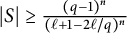
Theorem 1.2 Let $S \subset \mathbb {F}_q^n$ . Suppose that S is an $(n, d)$ -BRK-type set of degree $\ell $ , where $\ell \geq 1$ . Then $|S| \geq \frac {(q-1)^n}{(\ell + 1 - 2\ell /q)^n}$ .

The proof of Theorem 1.2 is an extension of our proof for Theorem 1.1: if $|S| < \frac {(q-1)^n}{(\ell + 1 - 2\ell /q)^n}$ , we can construct an analogous nonzero polynomial in $\rho $ that vanishes on all $\rho \in (\mathbb {F}_q \setminus \{0\})^{n-d}$ with high multiplicity. This polynomial is shown to have too many zeros, counting multiplicities.

In Section 2, we set notation, present our main tools (the polynomial method, Hasse derivatives and multiplicities, and the graded lexicographic order), and give a few preliminary results. We then prove Theorem 1.1 via the polynomial method in Section 3. In Section 4, we upgrade this to Theorem 1.2 using the method of multiplicities.

2 Preliminaries

2.1 Notation

We briefly introduce some notation which we will use throughout. We fix n and d as in Definition 1.2 and use m in lemmas which will later be applied to both cases $m=n$ and $m=d$ . For $x = (x_1, \dots , x_m) \in \mathbb {F}_q^m$ and $\alpha = (\alpha _1, \dots , \alpha _m) \in \mathbb {Z}_{\geq 0}^m$ , where $m \in \mathbb {N}$ , we write

$$\begin{align*}x^\alpha = \prod_{i=1}^m x_i^{\alpha_i}.\end{align*}$$ x Superscript alpha Baseline equals product Underscript i equals 1 Overscript m Endscripts x Subscript i Superscript alpha Super Subscript i Superscript Baseline period

If we also have $\beta = (\beta _1, \dots , \beta _m)$ , the multi-index binomial coefficients are defined by

$$\begin{align*}\binom{\alpha}{\beta} = \prod_{i=1}^n \binom{\alpha_i}{\beta_i},\end{align*}$$ StartBinomialOrMatrix alpha Choose beta EndBinomialOrMatrix equals product Underscript i equals 1 Overscript n Endscripts StartBinomialOrMatrix alpha Subscript i Baseline Choose beta Subscript i Baseline EndBinomialOrMatrix comma

with the convention that $\binom {\alpha }{\beta } = 0$ if $\alpha _i < \beta _i$ for any i. We say that the magnitude of the exponent $\alpha $ is $|\alpha | = \sum _{i=1}^m \alpha _i$ . For $\alpha = (\alpha _1, \dots , \alpha _n) \in \mathbb {Z}_{\geq 0}^n$ , we write

$$\begin{align*}\alpha' = (\alpha_{d+1}, \dots, \alpha_n)\end{align*}$$

to denote taking only the final $n-d$ coordinates of $\alpha $ .

Let $f(x)= \sum _{\alpha \in \mathbb {Z}_{\geq 0}^m} c_\alpha x^\alpha \in \mathbb {F}_q[x_1, \dots , x_m]$ . We say that the degree of f is

$$\begin{align*}\deg f := \max\{|\alpha|: c_\alpha \neq 0\}.\end{align*}$$

We say that f is nonzero if there exists $\alpha $ so that $c_\alpha \neq 0$ ; this is not, in general, equivalent to f vanishing everywhere, as it is possible for nonzero polynomials of degree greater than or equal to q to vanish everywhere.

Finally, we define a piece of notation which will be useful later on. For polynomials $\{f_i(x)\}_{i=1}^n \subset \mathbb {F}_q[x_1, \dots , x_d]$ and $\beta \in \mathbb {Z}_{\geq 0}^n$ , we define

$$\begin{align*}E_\beta(f_1(x), \dots, f_n(x)) := \prod_{i=1}^n (f_i(x))^{\beta_i}.\end{align*}$$

This is the polynomial obtained by substituting the tuple $(y_1 = f_1(x), \dots , y_n = f_n(x))$ into the monomial $y^\beta $ . In particular, if each $f_i(x)$ is a monomial in x, $E_\beta (f_1(x), \dots , f_n(x))$ is also a monomial.

2.2 The polynomial method

Dvir’s proof [Reference Dvir3] that Kakeya sets in $\mathbb {F}_q^n$ have cardinality bounded below by $c_nq^n$ uses what is now known as the polynomial method and is centreed around the idea that a polynomial of low degree cannot have too many zeros. If a Kakeya set K is too small, one can obtain a nonzero polynomial of low degree that vanishes at every point in K. Evaluating this polynomial on the parameterized lines contained in K, we then obtain a single-variable polynomial of low degree that is zero everywhere, and thus is the zero polynomial. From this, it can be shown that our original polynomial must also vanish at too many points outside of K, which gives a contradiction.

We present two essential tools used in the polynomial method. The first is a statement about how small a set needs to be to guarantee that we can find a nonzero polynomial vanishing on it. This is essentially a statement about solution sets of systems of homogeneous linear equations, as we can treat coefficients in polynomials vanishing at certain points as variables in a system of linear equations.

Lemma 2.1 [Reference Guth6, Lemma 2.3]

Let $S \subset \mathbb {F}_q^n$ . If $|S| < \binom {D + n}{n}$ , there exists a nonzero polynomial $f \in \mathbb {F}_q[x_1, \dots , x_n]$ , with $\deg f \leq D$ , such that $f(s) = 0$ for all $s \in S$ .

The Schwartz–Zippel lemma is the second main tool in the polynomial method and gives a bound on the number of zeros a polynomial can have over a Cartesian product of a set.

Lemma 2.2 [Reference Schwartz11, Reference Zippel16]

Let $A \subset \mathbb {F}_q$ . If $f \in \mathbb {F}_q[x_1, \dots , x_m]$ satisfies $\deg f \leq d$ , then

$$\begin{align*}|\{x \in A^m: f(x) = 0\}| \leq d|A|^{m-1}.\end{align*}$$

2.3 Hasse derivatives and multiplicities

The method of multiplicities extends the polynomial method and uses the idea that polynomials of not too high degree cannot vanish at too many points with high multiplicity. This allows us to work with polynomials of degree greater than the size of the field and thus obtain sharper lower bounds on quantities of interest. The notion of the multiplicity with which a polynomial vanishes at a point uses Hasse derivatives, which we define below.

Definition 2.1 Let $f(x) \in \mathbb {F}_q[x_1, \dots , x_m]$ , and let $\beta \in \mathbb {Z}_{\geq 0}^m$ . We define the $\beta $ -th Hasse derivative of f, denoted by $f^{(\beta )}$ , to be the coefficient of $y^\beta $ in $f(x+y)$ . Then

$$\begin{align*}f(x+y) = \sum_{\beta} f^{(\beta)}(x) y^\beta.\end{align*}$$

In our proof of Theorem 1.2, we use the explicit form for Hasse derivatives, which we also state here.

Lemma 2.3 [Reference Trainor12, Lemma 2.9]

Let $f(x) = \sum _{\alpha } c_\alpha x^\alpha \in \mathbb {F}_q[x_1, \dots , x_m]$ , and let $\beta \in \mathbb {Z}_{\geq 0}^m$ . Then

$$\begin{align*}f^{(\beta)}(x) = \sum_{\alpha} c_\alpha \binom{\alpha}{\beta} x^{\alpha-\beta}.\end{align*}$$

Now we define what it means for a polynomial over $\mathbb {F}_q^m$ to vanish at a point with a certain multiplicity. If we have a polynomial $p(x) \in \mathbb {C}[x]$ , $p(x)$ vanishes at a point $a \in \mathbb {C}$ with multiplicity k if $(x-a)^k \mid p(x)$ and $(x-a)^{k+1} \nmid p(x)$ . Equivalently, $p(x)$ vanishes at $a \in \mathbb {C}$ with multiplicity k if $p^{(k-1)}(a) = 0$ and $p^{(k)}(a) \neq 0$ . This idea of using derivatives to measure the multiplicity with which a polynomial vanishes at a point can be extended to polynomials over finite fields and their Hasse derivatives.

Definition 2.2 Let $a \in \mathbb {F}_q^m$ , and let $A \subset \mathbb {F}_q^m$ . We define the multiplicity of $f(x) \in \mathbb {F}_1[x_1, \dots , x_m]$ at a to be

$$\begin{align*}\operatorname{\mathrm{mult}}(f,a) := \sup\{M \in \mathbb{Z}_{\geq 0}: f^{(\beta)}(a) = 0 \text{ for all } \beta \in \mathbb{Z}_{\geq 0}^m \text{ with } |\beta| < M\}. \end{align*}$$

If $\operatorname {\mathrm {mult}}(f, a) \geq M$ for all $a \in A$ , we say that f vanishes on the set A with multiplicity M.

The following two lemmas provide lower bounds on the behavior of multiplicities under taking Hasse derivatives and under function composition.

Lemma 2.4 [Reference Dvir, Kopparty, Saraf and Sudan4, Lemma 2.4]

Let $P \in \mathbb {F}_q[x_1, \dots , x_n]$ and $\beta \in \mathbb {Z}_{\geq 0}^n$ . Then for $a \in \mathbb {F}_q^n$ ,

$$\begin{align*}\operatorname{\mathrm{mult}}(P^{(\beta)}, a) \geq \operatorname{\mathrm{mult}}(P, a) - |\beta|.\end{align*}$$

Lemma 2.5 [Reference Dvir, Kopparty, Saraf and Sudan4, Proposition 2.5]

Let $P(x) \in \mathbb {F}_q[x_1, \dots , x_m]$ , $Q(y) := (Q_1(y), \dots ,$ $Q_m(y)) \in (\mathbb {F}_q[y_1, \dots , y_j])^m$ , and $a \in \mathbb {F}_q^j$ . Then

$$\begin{align*}\operatorname{\mathrm{mult}}(P \circ Q, a) \geq \operatorname{\mathrm{mult}}(P, Q(a)).\end{align*}$$

Finally, we present multiplicity-enhanced versions of the two main tools used in the polynomial method. The first is an extension of Lemma 2.1 and states how small a set must be to guarantee the existence of a polynomial of not too high degree vanishing on our set with a given multiplicity.

Lemma 2.6 [Reference Dvir, Kopparty, Saraf and Sudan4, Proposition 3.1]

Let $A \subset \mathbb {F}_q^n$ . If

$$\begin{align*}\binom{M + n - 1}{n} \cdot |A| < \binom{D + n}{n},\end{align*}$$

then there exists a nonzero polynomial $P \in \mathbb {F}_q[x_1, \dots , x_n]$ of degree at most D vanishing on A with multiplicity M.

The second main tool is a multiplicity-enhanced version of the Schwartz–Zippel lemma (Lemma 2.2). This gives the same upper bound on the number of zeros of a polynomial as the Schwartz–Zippel lemma, but here we count zeros with their multiplicity.

Lemma 2.7 [Reference Dvir, Kopparty, Saraf and Sudan4, Lemma 2.7]

Let $A \subset \mathbb {F}_q$ . Let $P \in \mathbb {F}_q[x_1, \dots , x_n]$ be a nonzero polynomial of degree d. Then

$$\begin{align*}\sum_{a \in A^n} \operatorname{\mathrm{mult}}(P, a) \leq d|A|^{n-1}.\end{align*}$$

2.4 Vanishing multiplicities in the context of $(n,d)$ -BRK-type sets of degree $\ell $

In this section, we adapt some of the methods of [Reference Trainor12] specific to the constituent hypersurfaces in BRK-type sets to analogous methods for the d-dimensional subsets in $(n,d)$ -BRK-type sets.

The first lemma is an analogue of [Reference Trainor12, Lemma 2.7], which states that if a polynomial of sufficiently low degree vanishes on an $(n-1)$ -dimensional subset of degree $\ell $ with high multiplicity, then it must be the zero polynomial. We observe that an identical result holds for our $(n-d)$ -dimensional subsets, with an identical proof to [Reference Trainor12, Lemma 2.7], using Lemma 2.5 as a generalization of [Reference Trainor12, Lemma 2.3].

Lemma 2.8 Let $\ell \in \mathbb {N}$ with $1 \leq \ell < q$ , and let $\{g_i\}_{i=1}^{n-d} \subset \mathbb {F}_q[t_1, \dots , t_d]$ be polynomials of degree $\ell $ . For $\rho \in (\mathbb {F}_q \setminus \{0\})^{n-d}$ and $a \in \mathbb {F}_q^n$ , let

$$\begin{align*}C := \{a + (t, \rho_1 g_1(t), \dots, \rho_{n-k} g_{n-d}(t)): t \in \mathbb{F}_q^{d}\}.\end{align*}$$

Let $k, D, M \in \mathbb {N}$ be such that

(2.1) $$ \begin{align} \ell(D - \omega) < (M- \omega)q \end{align} $$

for $\omega = k-1$ . Suppose that f is a nonzero polynomial of degree at most D vanishing on C with multiplicity M. Let $f^{(\beta )}$ denote the Hasse derivative of f of order $\beta \in \mathbb {Z}_{\geq 0}^n$ , and let

$$\begin{align*}f_{\beta, \rho}(s) := f^{(\beta)}(a + (s, \rho_1g_1(s), \dots, \rho_{n-d}g_{n-d}(s))).\end{align*}$$

Then for $|\beta | < k$ , $f_{\beta , \rho }$ is the zero polynomial.

Proof [Reference Trainor12, Proof of Lemma 2.7] Let $\beta \in \mathbb {Z}_{\geq 0}^m$ , with $|\beta | < k$ . Since f has degree at most D, $f^{(\beta )}$ has degree at most $D - |\beta |$ , so that $f_{\beta , \rho }$ has degree at most $\ell (D - |\beta |)$ . Additionally, since f vanishes on C with multiplicity M, by Lemma 2.4, we have that $f^{(\beta )}$ vanishes on C with multiplicity at least $M - |\beta |$ . Then Lemma 2.5 implies that $f_{\beta , \rho }$ vanishes on $\mathbb {F}_q^d$ with multiplicity at least $M - |\beta |$ .

Notice that (2.1) must also hold for all $\omega \leq k-1$ , and so in particular must hold for $\omega = |\beta |$ . It follows that

$$ \begin{align*} \sum_{s \in \mathbb{F}_q^d} \operatorname{\mathrm{mult}}(f_{\beta, \rho}, s) \geq (M - |\beta|) q^d> \ell(D -|\beta|) q^{d-1} \geq \deg{f_{\beta, \rho}} q^{d-1}. \end{align*} $$

Applying the multiplicity-enhanced Schwartz–Zippel lemma (Lemma 2.7), we see that $f_{\beta , \rho }$ must be the zero polynomial.

In our proof of Theorem 1.2, we encounter a family of polynomials $P_\gamma (\rho )$ that vanish everywhere and are “almost” the Hasse derivatives of a polynomial up to a multiplicity k. We would like to use this to conclude that our original polynomial vanishes everywhere with multiplicity k. To do this, we use the following lemma. In a sense, this is a higher-dimensional analogue of [Reference Trainor12, Lemma 3.1]; however, this differs because our dilation parameter only impacts the final $n-d$ coordinates in our subset.

Lemma 2.9 Let $k, n \in \mathbb {N}$ , let $\{b_\alpha \}_{\alpha \in \mathbb {Z}^n} \in \mathbb {F}_q$ , and let $c \in \mathbb {F}_q^{n-d}$ . Suppose that for all $\beta \in \mathbb {Z}_{\geq 0}^n$ with $|\beta | < k$ and each $t \in (\mathbb {F}_q \setminus \{0\})^d$ , the value

$$\begin{align*}f_{\beta}(t) = \sum_{|\alpha| < k(q-1)} b_\alpha \binom{\alpha}{\beta} c^{\alpha' - \beta'}t^{\alpha' - \beta'}\end{align*}$$ f Subscript beta Baseline left parenthesis t right parenthesis equals sigma summation Underscript StartAbsoluteValue alpha EndAbsoluteValue less than k left parenthesis q minus 1 right parenthesis Endscripts b Subscript alpha Baseline StartBinomialOrMatrix alpha Choose beta EndBinomialOrMatrix c Superscript alpha prime minus beta prime Baseline t Superscript alpha prime minus beta prime

is zero, where $\alpha ' = (\alpha _{d+1}, \dots , \alpha _{n})$ (and similarly for $\beta '$ .) Then $b_\alpha = 0$ for all $\alpha $ .

Proof By a change of variables $s_i = c_i t_i$ , we obtain polynomials

$$\begin{align*}\tilde{f}_\beta(s) := \sum_{|\alpha| < k(q-1)} b_\alpha \binom{\alpha}{\beta} s^{\alpha' - \beta'},\end{align*}$$

which are zero for all $s \in (\mathbb {F}_q \setminus \{0\})^d$ whenever $|\beta | < k$ . Consider $\tilde {f}_0(s) = $ $\sum _{|\alpha | < k(q-1)} b_\alpha s^\alpha $ , and let $\beta ' \in \mathbb {Z}_{\geq 0}^{n-d}$ . The $\beta '$ -th Hasse derivative of $\tilde {f}_0$ is

(2.2) $$ \begin{align} \tilde{f}_0^{(\beta')}(s) = \sum_{|\alpha| < k(q-1)} b_\alpha \binom{\alpha'}{\beta'} s^{\alpha' - \beta'}. \end{align} $$

Taking $\beta = (0, \dots , 0, \beta ')$ , we have that

$$\begin{align*}\binom{\alpha}{\beta} = \prod_{i=1}^n \binom{\alpha_i}{\beta_i} = \Big(\prod_{i=1}^d \binom{\alpha_i}{0} \Big) \Big(\prod_{j=1}^{n-d} \binom{\alpha_{j+d}}{\beta^{\prime}_j}\Big) = 1 \cdot \binom{\alpha'}{\beta'}.\end{align*}$$

It follows that $\tilde {f}_0^{(\beta ')}(s) = \tilde {f}_{\beta }(s)$ ; observe also that $|\beta | = |\beta '| < k$ . Then $\tilde {f}_0^{(\beta ')}(s)$ is zero for all $s \in (\mathbb {F}_q \setminus \{0\})^d$ . Since $\beta '$ was arbitrary, $\tilde {f}_0$ is thus a polynomial of degree less than $k(q-1)$ vanishing on $(\mathbb {F}_q \setminus \{0\})^d$ with multiplicity k, and hence is identically zero by Lemma 2.7.

2.5 The graded lexicographic order on $\boldsymbol{\mathbb {F}_q[x_1, \dots , x_d]}$ and some associated lemmas

In our proofs, we isolate for specific coefficients of polynomials after evaluation on our constituent subsets. To do this, we want a notion of a “leading coefficient” of a polynomial in several variables, which requires a total order on the associated monic monomials. For this, we use the graded lexicographic order on monomials. This begins by sorting monic monomials by their total degree, which is necessary as the polynomials that determine our surfaces are only fixed in the highest homogeneous part. We then use the lexicographical ordering to distinguish between distinct monomials of each total degree; this allows us to always select a unique highest monomial in any polynomial. The following results are standard and can be seen from, for example, [Reference Cox, Little and O’Shea2, Chapter 2.2]. We include their proofs for completeness.

Definition 2.3 Let $\alpha , \beta \in \mathbb {Z}_{\geq 0}^d$ . We write $x^{\alpha } \prec x^{\beta }$ whenever $x^{\alpha } \prec x^{\beta }$ with respect to the graded lexicographical order. That is, $x^{\alpha } \prec x^{\beta }$ if $|\alpha | < |\beta |$ , or if $|\alpha | = |\beta |$ and $\alpha < \beta $ with respect to the lexicographical order.

We extend this to $\mathbb {F}_q[x_1, \dots , x_m]$ as follows: we write $LM(f)$ for the leading monomial of $f(x) \in \mathbb {F}_q[x_1, \dots , x_d]$ , and we say that $g(x) \prec f(x)$ if $LM(g) \prec LM(f)$ .

With this partial order in hand, we consider how it behaves under various operations on polynomials.

Remark 2.10 It is immediate from the definition of $\prec $ that if $g(x) \prec f(x)$ and $h(x) \prec f(x)$ , then $g(x) + h(x) \prec f(x)$ .

Next, we show that $\prec $ behaves as expected under monomial multiplication.

Lemma 2.11 If $x^\beta \prec x^\gamma $ , then $x^{\alpha + \beta } \prec x^{\alpha + \gamma }$ .

Proof If $|\beta | < |\gamma |$ , the result follows since $|\alpha + \beta | = |\alpha | + |\beta | < |\alpha | + |\gamma | = |\alpha + \gamma |$ . Otherwise, $|\alpha + \beta | = |\alpha + \gamma |$ , and there exists a minimal j so that $\beta _j < \gamma _j$ . Then the exponent of $x_j$ in $x^{\alpha + \beta }$ is $\alpha _j + \beta _j$ , which is strictly less than $\alpha _j + \gamma _j$ , so that $\alpha + \beta < \alpha + \gamma $ with respect to the lexicographical order.

This can be extended to polynomial multiplication: monomial dominance with respect to $\prec $ is preserved under arbitrary products of polynomials, and no cancellation occurs at the highest term. We state this formally below.

Lemma 2.12 Let $\{f_i(x)\}_{i=1}^N \subset \mathbb {F}_q[x_1, \dots , x_n]$ . Then

$$\begin{align*}LM\left(\prod_{i=1}^N f_i(x)\right) = \prod_{i=1}^N LM(f_i(x)).\end{align*}$$ StartLayout 1st Row upper L upper M left parenthesis product Underscript i equals 1 Overscript upper N Endscripts f Subscript i Baseline left parenthesis x right parenthesis right parenthesis equals product Underscript i equals 1 Overscript upper N Endscripts upper L upper M left parenthesis f Subscript i Baseline left parenthesis x right parenthesis right parenthesis period EndLayout

Proof We proceed by induction on N and begin with the $N=2$ case. Suppose that $LM(f_1(x)) = a_{\alpha } x^{\alpha }$ and $LM(f_2(x)) = b_{\beta } x^{\beta }$ . That is, we write $f_1(x) =a_{\alpha } x^{\alpha } + \sum _{\gamma \in A} a_{\gamma } x^{\gamma }$ and $f_2(x) = b_{\beta } x^{\beta } + \sum _{\mu \in B} b_{\mu } x^{\mu }$ , where $a_{\alpha } \neq 0$ , $b_{\beta } \neq 0$ , $x^{\gamma } \prec x^{\alpha }$ for all $\gamma \in A$ , and $x^{\mu } \prec x^{\beta }$ for all $\mu \in B$ . Then

$$ \begin{align*} f_1(x)f_2(x) &= \Big(a_\alpha x^\alpha + \sum_{\gamma \in A} a_{\gamma} x^{\gamma}\Big)\Big(b_\beta x^\beta + \sum_{\mu \in B} b_{\mu} x^{\mu}\Big) \\ &= a_\alpha b_\beta x^{\alpha + \beta} + g(x), \end{align*} $$

StartLayout 1st Row 1st Column f 1 left parenthesis x right parenthesis f 2 left parenthesis x right parenthesis 2nd Column equals left parenthesis a Subscript alpha Baseline x Superscript alpha Baseline plus sigma summation Underscript gamma element of upper A Endscripts a Subscript gamma Baseline x Superscript gamma Baseline right parenthesis left parenthesis b Subscript beta Baseline x Superscript beta Baseline plus sigma summation Underscript mu element of upper B Endscripts b Subscript mu Baseline x Superscript mu Baseline right parenthesis 2nd Row 1st Column Blank 2nd Column equals a Subscript alpha Baseline b Subscript beta Baseline x Superscript alpha plus beta Baseline plus g left parenthesis x right parenthesis comma EndLayout

where

$$\begin{align*}g(x) = a_\alpha \sum_{\mu \in B} b_\mu x^{\alpha + \mu} + b_\beta \sum_{\gamma \in A} a_\gamma x^{\gamma + \beta} +\sum_{\substack{\gamma \in A \\ \mu \in B}} a_{\gamma} b_{\mu} x^{\gamma + \mu}.\end{align*}$$

Lemma 2.11 implies that $x^{\alpha + \mu } \prec x^{\alpha + \beta }$ and $x^{\gamma + \mu } \prec x^{\gamma + \beta } \prec x^{\alpha + \beta }$ for all $\gamma \in A$ and all ${\mu \in B}$ , so that $g(x) \prec x^{\alpha + \beta }$ , as desired.

Now, suppose that the result holds for a product of N polynomials, with $LM(f_i(x)) = c_{\alpha ^i} x^{\alpha ^i}$ , and consider $\prod _{i=1}^{N+1} f_i(x) = \Big (\prod _{i=1}^N f_i(x)\Big )f_{N+1}(x)$ . By the inductive hypothesis,

$$\begin{align*}\prod_{i=1}^N f_i(x) = \Big(\prod_{i=1}^N c_{\alpha^i}\Big) x^{\sum_{i=1}^N \alpha^i} + G(x)\end{align*}$$

for some $G(x) \in \mathbb {F}_q[x_1, \dots , x_n]$ , where $G(x) \prec x^{\sum _{i=1}^N \alpha ^i}$ . The $N=2$ case then implies that

$$\begin{align*}\prod_{i=1}^{N+1} f_i(x) = \Biggl(\Big(\prod_{i=1}^N c_{\alpha^i}\Big) x^{\sum_{i=1}^N \alpha^i} + G(x)\Biggr)f_{N+1}(x) = \Big(\prod_{i=1}^{N+1} c_{\alpha^i}\Big) x^{\sum_{i=1}^{N+1} \alpha^i} + g(x)\end{align*}$$

for some $g(x)$ , where $g(x) \prec x^{\sum _{i=1}^{N+1} \alpha ^i}$ . By induction, the result holds for all N.

From this, it follows that in fact $\prec $ is preserved under polynomial multiplication.

Corollary 2.13 Suppose that $f(x) \prec g(x)$ . For any $h(x) \in \mathbb {F}_q[x_1, \dots , x_n]$ , $f(x)h(x) \prec g(x)h(x)$ .

Proof Write $f(x) = a x^\alpha +F(x)$ , $g(x) = bx^\beta + G(x)$ , and $h(x) = c x^\gamma + H(x)$ , where $a,b,$ and c are nonzero, $F(x) \prec x^\alpha $ , $G(x) \prec x^\beta $ , and $H(x) \prec x^\gamma $ . Then, by Lemma 2.12, we have

$$\begin{align*}f(x)h(x) = acx^{\alpha + \gamma} + f_1(x),\end{align*}$$

for some $f_1(x)$ with $f_1(x) \prec x^{\alpha + \gamma }$ , and

$$\begin{align*}g(x)h(x) = bcx^{\beta + \gamma} + f_2(x)\end{align*}$$

for some $f_2(x)$ with $f_2(x) \prec x^{\beta + \gamma }$ . By the definition of $f(x) \prec g(x)$ , $x^\alpha \prec x^\beta $ ; Lemma 2.11 then implies that $x^{\alpha + \gamma } \prec x^{\beta + \gamma }$ , and the result follows.

Monomial dominance with respect to $\prec $ is also often preserved with respect to taking Hasse derivatives, in the case where each input term is itself some polynomial in x. We state and prove such a result for monomials below, and we use the notation defined in Section 2.1.

Corollary 2.14 Let $\{\alpha ^i\}_{i=1}^n \subset \mathbb {Z}_{\geq 0}^{n}$ and $\beta ^1, \beta ^2 \in \mathbb {Z}_{\geq 0}^n$ , and suppose that $E_{\beta ^1}(x^{\alpha ^1}, \dots ,$ $x^{\alpha ^{n}}) \prec E_{\beta ^2}(x^{\alpha ^1}, \dots , x^{\alpha ^{n}})$ . Suppose additionally that $\gamma \in \mathbb {Z}_{\geq 0}^n$ is such that $\beta ^1 - \gamma , \beta ^2 - \gamma \in \mathbb {Z}_{\geq 0}^n$ . Then

$$\begin{align*}E_{\beta^1 - \gamma}(x^{\alpha^1}, \dots, x^{\alpha^{n}}) \prec E_{\beta^1 - \gamma}(x^{\alpha^1}, \dots, x^{\alpha^{n}}).\end{align*}$$

Proof This is a consequence of the fact that

$$\begin{align*}E_{\beta - \gamma}(x^{\alpha^1}, \dots, x^{\alpha^{n}})E_{\gamma}(x^{\alpha^1}, \dots, x^{\alpha^{n}}) = E_{\beta}(x^{\alpha^1}, \dots, x^{\alpha^{n}})\end{align*}$$

for any $\beta \in \mathbb {Z}_{\geq 0}^n$ and any $\gamma \in \mathbb {Z}_{\geq 0}^n$ with $\beta - \gamma \in \mathbb {Z}_{\geq 0}^n$ , and we prove the contrapositive.

Since both polynomials we compare are monic monomials in x, and $\prec $ gives a total order on such monomials, they are always either equal or comparable via $\prec $ . If $E_{\beta ^1 - \gamma }(x^{\alpha ^1}, \dots , x^{\alpha ^{n}}) = E_{\beta ^2 - \gamma }(x^{\alpha ^1}, \dots , x^{\alpha ^{n}})$ , then

$$\begin{align*}E_{\beta^1}(x^{\alpha^1}, \dots, x^{\alpha^{n}}) = E_{\beta^2}(x^{\alpha^1}, \dots, x^{\alpha^{n}}).\end{align*}$$

If $E_{\beta ^2 - \gamma }(x^{\alpha ^1}, \dots , x^{\alpha ^{n}}) \prec E_{\beta ^1 - \gamma }(x^{\alpha ^1}, \dots , x^{\alpha ^{n}})$ , Corollary 2.13 implies that

$$\begin{align*}E_{\beta^2}(x^{\alpha^1}, \dots, x^{\alpha^{n}}) \prec E_{\beta^1 }(x^{\alpha^1}, \dots, x^{\alpha^{n}}).\end{align*}$$

In both cases, we do not have

$$\begin{align*}E_{\beta^1}(x^{\alpha^1}, \dots, x^{\alpha^{n}}) \prec E_{\beta^2}(x^{\alpha^1}, \dots, x^{\alpha^{n}}).\\[-31pt] \end{align*}$$

3 Proof of Theorem 1.1

Let S be an $(n,d)$ -BRK-type set, and let $t = (t_1, \dots , t_d)$ . Let $\{h_i(t)\}_{i=1}^{n-d}$ and $\Gamma _\rho $ be as in Definition 1.2. Suppose, toward contradiction, that $|S| < \binom {\left \lfloor (q-1)/\ell \right \rfloor + n}{n}$ . By Lemma 2.1, there exists a nonzero polynomial $f \in \mathbb {F}_q[x_1, \dots , x_n]$ with $\deg f \leq \left \lfloor \frac {q-1}{\ell }\right \rfloor $ vanishing on S. We write $f(x) = \sum _{\beta \in B} b_\beta x^\beta $ , where $B \subset \mathbb {Z}_{\geq 0}^n$ is the set of multi-indices $\beta $ with $b_\beta \neq 0$ .

We begin by considering the polynomials $\{h_i(t)\}_{i=1}^{n-d}$ . For each i, we may write $h_i(t) = c_{\alpha ^i} t^{\alpha ^i} + H_i(t)$ , where $t^{\alpha ^i} \succ H_i(t)$ . We consider $LM(f(t, t^{\alpha ^1}, \dots , t^{\alpha ^{n-d}}))$ , the leading monomial obtained by evaluating f at $(t, t^{\alpha ^1}, \dots , t^{\alpha ^{n-d}})$ and considering this as a polynomial in t. That is, we write

$$\begin{align*}f(x) = \sum_{j=1}^N b_{\beta^j} x^{\beta^j} + F(x)\end{align*}$$ f left parenthesis x right parenthesis equals sigma summation Underscript j equals 1 Overscript upper N Endscripts b Subscript beta Sub Superscript j Baseline x Superscript beta Super Superscript j Baseline plus upper F left parenthesis x right parenthesis

for some $N \in \mathbb {N}$ , where the $\beta ^j$ satisfy

$$\begin{align*}E_{\beta^i}(t, t^{\alpha^1}, \dots, t^{\alpha^{n-d}}) = E_{\beta^j}(t, t^{\alpha^1}, \dots, t^{\alpha^{n-d}}) \end{align*}$$

for all $1 \leq i, j \leq N$ , and

$$\begin{align*}E_{\beta^1}(t, t^{\alpha^1}, \dots, t^{\alpha^{n-d}}) \succ F(t, t^{\alpha^1}, \dots, t^{\alpha^{n-d}}). \end{align*}$$

Now, let $\rho \in (\mathbb {F}_q \setminus \{0\})^{n-d}$ . Since f vanishes on S, we must have

$$\begin{align*}f_\rho(t) := f(\Gamma_\rho(t)) = 0\end{align*}$$

for all $t \in \mathbb {F}_q^d$ . Since the input in each coordinate is a polynomial of total degree at most $\ell $ , it follows that $\deg f_\rho \leq \deg f \cdot \ell \leq q-1$ , and thus that $f_\rho (t)$ is the zero polynomial.

Applying Lemma 2.12 to $f_\rho (t)$ , we obtain

$$ \begin{align*} f_\rho(t) &= \sum_{\beta \in B} b_\beta (\Gamma_\rho(t))^\beta \\ &= \sum_{\beta \in B} b_\beta\Big(E_\beta(t, \rho_1 c_{\alpha^1}t^{\alpha^1}, \dots, \rho_{n-d} c_{\alpha^{n-d}} t^{\alpha^{n-d}}) + F_{\rho, \beta}(t)\Big)\\ &= \sum_{\beta \in B} b_\beta\Big(\Big(\prod_{i=1}^{n-d} \rho_i^{\beta_{i+d}}c_{\alpha^i}^{\beta_{i+d}}\Big) E_\beta(t, t^{\alpha^1}, \dots, t^{\alpha^{n-d}}) + F_{\rho, \beta}(t)\Big), \end{align*} $$

StartLayout 1st Row 1st Column f Subscript rho Baseline left parenthesis t right parenthesis 2nd Column equals sigma summation Underscript beta element of upper B Endscripts b Subscript beta Baseline left parenthesis normal upper Gamma Subscript rho Baseline left parenthesis t right parenthesis right parenthesis Superscript beta Baseline 2nd Row 1st Column Blank 2nd Column equals sigma summation Underscript beta element of upper B Endscripts b Subscript beta Baseline left parenthesis upper E Subscript beta Baseline left parenthesis t comma rho 1 c Subscript alpha Sub Superscript 1 Subscript Baseline t Superscript alpha Super Superscript 1 Superscript Baseline comma ellipsis comma rho Subscript n minus d Baseline c Subscript alpha Sub Superscript n minus d Subscript Baseline t Superscript alpha Super Superscript n minus d Superscript Baseline right parenthesis plus upper F Subscript rho comma beta Baseline left parenthesis t right parenthesis right parenthesis 3rd Row 1st Column Blank 2nd Column equals sigma summation Underscript beta element of upper B Endscripts b Subscript beta Baseline left parenthesis left parenthesis product Underscript i equals 1 Overscript n minus d Endscripts rho Subscript i Superscript beta Super Subscript i plus d Superscript Baseline c Subscript alpha Sub Superscript i Subscript Superscript beta Super Subscript i plus d Superscript Baseline right parenthesis upper E Subscript beta Baseline left parenthesis t comma t Superscript alpha Super Superscript 1 Superscript Baseline comma ellipsis comma t Superscript alpha Super Superscript n minus d Superscript Baseline right parenthesis plus upper F Subscript rho comma beta Baseline left parenthesis t right parenthesis right parenthesis comma EndLayout

where $F_{\rho , \beta }(t) \prec E_{\beta; \alpha ^1, \dots , \alpha ^{n-d}}(t) $ for each $\beta $ . By our choice of $\{\beta ^j\}_{j=1}^N$ , the leading coefficient of $f_\rho (t)$ is thus given by

$$\begin{align*}P(\rho) = \sum_{j=1}^N b_{\beta^j} \rho^{(\beta^j)'}c^{(\beta^j)'},\end{align*}$$

where $(\beta ^j)'$ are defined as in Section 2.1. This is zero, since $f_\rho $ is the zero polynomial. But $\rho $ was arbitrary: P is thus a nonzero polynomial of total degree at most $\frac {q-1}{\ell }$ that vanishes at every $\rho \in (\mathbb {F}_q \setminus \{0\})^{n-d}$ . This is the desired contradiction, as Lemma 2.2 asserts that such a polynomial has no more than $\frac {(q-1)^{n-d}}{\ell } < (q-1)^{n-d}$ zeros in $(\mathbb {F}_q \setminus \{0\})^{n-d}$ .

4 Proof of Theorem 1.2

We obtain our lower bound on the cardinality of $(n,d)$ -BRK-type sets of degree $\ell $ from a sequence of lower bounds.

Lemma 4.1 Let S be an $(n,d)$ -BRK-type set of degree $\ell $ , and let $k \in \mathbb {N}$ be a multiple of q. Let $D = k(q-1) - 1$ and $M = (\ell + 1)k - 2\ell k/q$ . Then

$$\begin{align*}\binom{M + n - 1}{n} |S| \geq \binom{D + n}{n}.\end{align*}$$

Proof Suppose, again toward contradiction, that there exists $k \in \mathbb {N}$ , a multiple of q, so that for $D = k(q-1) - 1$ and $M = (\ell + 1)k - 2\ell k/q$ ,

$$\begin{align*}\binom{M + n - 1}{n} |S| < \binom{D + n}{n}.\end{align*}$$

By Lemma 2.6, there exists a nonzero polynomial $f \in \mathbb {F}_q[x_1, \dots , x_n]$ with $\deg f \leq D$ vanishing on S with multiplicity M. We again write $f(x) = \sum _{\beta \in B} b_\beta x^\beta $ , where $B \subset \mathbb {Z}_{\geq 0}^n$ is the set of multi-indices $\beta $ with $b_\beta \neq 0$ .

We again consider the polynomials $\{h_i(t)\}_{i=1}^{n-d}$ . For each i, we write $h_i(t) = c_{\alpha ^i} t^{\alpha ^i} + H_i(t)$ , where $t^{\alpha ^i} \succ H_i(t)$ . Define $c = (c_{\alpha ^1}, \dots , c_{\alpha ^{n-d}}) \in \mathbb {F}_q^{n-d}$ . We again consider $LM(f(t, t^{\alpha ^1}, \dots , t^{\alpha ^{n-d}}))$ , the leading monomial obtained by evaluating f at $(t, t^{\alpha ^1}, \dots , t^{\alpha ^{n-d}})$ and considering this as a polynomial in t. As in the proof of Theorem 1.1, we write

$$\begin{align*}f(x) = \sum_{j=1}^N b_{\beta^j} x^{\beta^j} + F(x),\end{align*}$$ f left parenthesis x right parenthesis equals sigma summation Underscript j equals 1 Overscript upper N Endscripts b Subscript beta Sub Superscript j Subscript Baseline x Superscript beta Super Superscript j Superscript Baseline plus upper F left parenthesis x right parenthesis comma

where the $\beta ^j$ satisfy

$$\begin{align*}E_{\beta^i}(t, t^{\alpha^1}, \dots, t^{\alpha^{n-d}}) = E_{\beta^j}(t, t^{\alpha^1}, \dots, t^{\alpha^{n-d}})\end{align*}$$

for all $1 \leq i, j \leq N$ , and

$$\begin{align*}E_{\beta^1}(t, t^{\alpha^1}, \dots, t^{\alpha^{n-d}}) \succ F(t, t^{\alpha^1}, \dots, t^{\alpha^{n-d}}).\end{align*}$$

Let $\rho \in (\mathbb {F}_q \setminus \{0\})^{n-d}$ . Since f vanishes on S with multiplicity M, we must have

$$\begin{align*}f_{\gamma, \rho}(t) := f^{(\gamma)}(\Gamma_\rho(t)) = 0\end{align*}$$

for all $t \in \mathbb {F}_q^d$ and all $|\gamma | < M$ . Since $\ell , D, M$ , and $\omega =k-1$ satisfy the inequality (2.1), Lemma 2.8 states that for $|\gamma | < k$ , $f_{\gamma , \rho }$ is the zero polynomial.

Fix some $|\gamma | < k$ . Applying Lemmas 2.3 and 2.12 to $f_{\gamma , \rho }(t)$ , we obtain

$$ \begin{align*} f_{\gamma, \rho}(t) &= \sum_{\substack{\beta \in B \\ \beta - \gamma \in \mathbb{Z}_{\geq 0}^n}} b_\beta \binom{\beta}{\gamma}\Big( \!\Big(\! \prod_{i=1}^{n-d} \rho_i^{\beta_{i+d} - \gamma_{i+d}}c_{\alpha^i}^{\beta_{i+d} - \gamma_{i+d}}\Big) E_{\beta - \gamma}(t, t^{\alpha^1}, \dots, t^{\alpha^{n-d}}) + F_{\rho, \beta, \gamma}(t)\Big), \end{align*} $$

StartLayout 1st Row 1st Column f Subscript gamma comma rho Baseline left parenthesis t right parenthesis 2nd Column equals sigma summation Underscript StartLayout 1st Row beta element of upper B 2nd Row beta minus gamma element of double struck upper Z Subscript greater than or equals 0 Superscript n Baseline EndLayout Endscripts b Subscript beta Baseline StartBinomialOrMatrix beta Choose gamma EndBinomialOrMatrix left parenthesis left parenthesis product Underscript i equals 1 Overscript n minus d Endscripts rho Subscript i Superscript beta Super Subscript i plus d Superscript minus gamma Super Subscript i plus d Superscript Baseline c Subscript alpha Sub Superscript i Subscript Superscript beta Super Subscript i plus d Superscript minus gamma Super Subscript i plus d Superscript Baseline right parenthesis upper E Subscript beta minus gamma Baseline left parenthesis t comma t Superscript alpha Super Superscript 1 Superscript Baseline comma ellipsis comma t Superscript alpha Super Superscript n minus d Superscript Baseline right parenthesis plus upper F Subscript rho comma beta comma gamma Baseline left parenthesis t right parenthesis right parenthesis comma EndLayout

where $F_{\rho , \beta , \gamma } \prec E_{\beta - \gamma }(t, t^{\alpha ^1}, \dots , t^{\alpha ^{n-k}})$ for all $\beta $ . To find the leading coefficient of $f_{\gamma , \rho }(t)$ , by Lemma 2.12, it thus suffices to compare $E_{\beta - \gamma }(t, t^{\alpha ^1}, \dots , t^{\alpha ^{n-k}})$ for all $\beta \in B$ with $\beta - \gamma \in \mathbb {Z}_{\geq 0}^n$ . If $\beta ^j - \gamma \in \mathbb {Z}_{\geq 0}^n$ for any j (without loss of generality, we assume $j=1$ ), Corollary 2.14 implies that the coefficient corresponding to the monomial $(t, t^{\alpha ^1}, \dots , t^{\alpha ^{n-k}})^{\beta ^1 - \gamma }$ is

$$\begin{align*}P_{\gamma}(\rho):= \sum_{j=1}^N b_{\beta^j} \binom{\beta^j}{\gamma} \rho^{(\beta^j)' - \gamma'} c^{(\beta^j)' - \gamma'} = \sum_{\substack{1 \leq j \leq N \\ \beta^j - \gamma \in \mathbb{Z}_{\geq 0}^n}} b_{\beta^j} \binom{\beta^j}{\gamma} \rho^{(\beta^j)' - \gamma'} c^{(\beta^j)' - \gamma'}\end{align*}$$

upper P Subscript gamma Baseline left parenthesis rho right parenthesis colon equals sigma summation Underscript j equals 1 Overscript upper N Endscripts b Subscript beta Sub Superscript j Baseline StartBinomialOrMatrix beta Superscript j Baseline Choose gamma EndBinomialOrMatrix rho Superscript left parenthesis beta Super Superscript j Superscript right parenthesis prime minus gamma prime Baseline c Superscript left parenthesis beta Super Superscript j Superscript right parenthesis prime minus gamma prime Baseline equals sigma summation Underscript StartLayout 1st Row 1 less than or equals j less than or equals upper N 2nd Row beta Superscript j Baseline minus gamma element of double struck upper Z Subscript greater than or equals 0 Superscript n Baseline EndLayout Endscripts b Subscript beta Sub Superscript j Baseline StartBinomialOrMatrix beta Superscript j Baseline Choose gamma EndBinomialOrMatrix rho Superscript left parenthesis beta Super Superscript j Superscript right parenthesis prime minus gamma prime Baseline c Superscript left parenthesis beta Super Superscript j Superscript right parenthesis prime minus gamma prime

and is zero, where we use that the $\beta ^j$ not included in the second sum satisfy $\binom {\beta ^j}{\gamma } = 0$ as in Lemma 2.3. Otherwise, $\binom {\beta ^j}{\gamma } = 0$ for all $1 \leq j \leq N$ , and hence in this case, we also have that $P_{\gamma }(\rho ) = 0$ .

Since $|\gamma | < k$ was arbitrary, Lemma 2.9 implies that each $b_{\beta ^j}$ is zero. This contradicts our initial assumption that each $b_\beta $ is nonzero.

Hence, for each $k \in \mathbb {N}$ , k a multiple of q, with $D = k(q-1)-1$ and $M = (\ell + 1) k - 2\ell k/q$ , we have

$$\begin{align*}|S| \geq \frac{\binom{D + n}{n}}{\binom{M + n - 1}{n}} = \frac{\prod_{i=1}^n (k(q-1) - 1 + i)}{\prod_{i=1}^n ((\ell + 1)k - 2\ell k/q + i - 1)}.\end{align*}$$

This holds for arbitrarily large k; taking the supremum over all such k, we obtain

$$\begin{align*}|S| \geq \frac{(q-1)^n}{((\ell + 1) - 2\ell/q)^n},\end{align*}$$ StartAbsoluteValue upper S EndAbsoluteValue greater than or equals StartFraction left parenthesis q minus 1 right parenthesis Superscript n Baseline Over left parenthesis left parenthesis script l plus 1 right parenthesis minus 2 script l divided by q right parenthesis Superscript n Baseline EndFraction comma

as desired.

Acknowledgements

I would like to thank Malabika Pramanik for her encouragement and many helpful suggestions.

Footnotes

This work was partially supported by an Undergraduate Student Research Award from the Natural Sciences and Engineering Research Council of Canada (NSERC).

References

Besicovitch, A. S. and Rado, R., A plane set of measure zero containing circumferences of every radius . J. Lond. Math. Soc. 43(1968), 717–719.Google Scholar

Cox, D. A., Little, J., and O’Shea, D., Ideals, varieties, and algorithms: An introduction to computational algebraic geometry and commutative algebra. 4th ed., Springer, New York, NY, 2015.Google Scholar

Dvir, Z., On the size of Kakeya sets in finite fields . J. Amer. Math. Soc. 22(2009), no. 4, 1093–1097.Google Scholar

Dvir, Z., Kopparty, S., Saraf, S., and Sudan, M., Extensions to the method of multiplicities, with applications to Kakeya sets and mergers . SIAM J. Comput. 42(2013), no. 6, 2305–2328.Google Scholar

Ellenberg, J. S., Oberlin, R., and Tao, T., The Kakeya set and maximal conjectures for algebraic varieties over finite fields . Mathematika 56(2010), no. 1, 1–25.Google Scholar

Guth, L., Polynomial methods in combinatorics, University Lecture Series, 64, American Mathematical Society, Providence, RI, 2016.Google Scholar

Kinney, J. R., A thin set of circles . Amer. Math. Monthly 75(1968), no. 10, 1077–1081.Google Scholar

Kolasa, L. and Wolff, T., On some variants of the Kakeya problem . Pacific J. Math. 190(1999), no. 1, 111–154.Google Scholar

Makhul, M., Warren, A., and Winterhof, A., The spherical Kakeya problem in finite fields . SIAM J. Discrete Math. 34(2020), no. 4, 2502–2509.Google Scholar

Saraf, S. and Sudan, M., An improved lower bound on the size of Kakeya sets over finite fields . Anal. PDE 1(2008), no. 3, 375–379.Google Scholar

Schwartz, J. T., Fast probabilistic algorithms for verification of polynomial identities . J. ACM 27(1980), no. 4, 701–717.Google Scholar

Trainor, C., BRK-type sets over finite fields . Finite Fields Appl. 105(2025), 102624, 23 pp.Google Scholar

Warren, A. and Winterhof, A., Conical Kakeya and Nikodym sets in finite fields . Finite Fields Appl. 59(2019), 185–198.Google Scholar

Wolff, T., A Kakeya-type problem for circles . Amer. J. Math. 119(1997), no. 5, 985–1026.Google Scholar

Wolff, T., Recent work connected with the Kakeya problem . In: Prospects in mathematics, Princeton, NJ, 1996, American Mathematical Society, Providence, RI, 1999, pp. 129–162.Google Scholar

Zippel, R., Probabilistic algorithms for sparse polynomials . In: Proceedings of the international symposium on symbolic and algebraic computation, Springer-Verlag, Berlin-New York, 1979, pp. 216–226.Google Scholar

Article contents

On an analogue of BRK-type sets in finite fields

Abstract

Keywords

MSC classification

Information

1 Introduction

Definition 1.1 [Reference Trainor12, Definition 1.1]

2 Preliminaries

2.1 Notation

2.2 The polynomial method

Lemma 2.1 [Reference Guth6, Lemma 2.3]

Lemma 2.2 [Reference Schwartz11, Reference Zippel16]

2.3 Hasse derivatives and multiplicities

Lemma 2.3 [Reference Trainor12, Lemma 2.9]

Lemma 2.4 [Reference Dvir, Kopparty, Saraf and Sudan4, Lemma 2.4]

Lemma 2.5 [Reference Dvir, Kopparty, Saraf and Sudan4, Proposition 2.5]

Lemma 2.6 [Reference Dvir, Kopparty, Saraf and Sudan4, Proposition 3.1]

Lemma 2.7 [Reference Dvir, Kopparty, Saraf and Sudan4, Lemma 2.7]

2.4 Vanishing multiplicities in the context of $(n,d)$ -BRK-type sets of degree $\ell $

2.5 The graded lexicographic order on $\boldsymbol{\mathbb {F}_q[x_1, \dots , x_d]}$ and some associated lemmas

3 Proof of Theorem 1.1

4 Proof of Theorem 1.2

Acknowledgements

Footnotes

References

Save article to Kindle

Save article to Dropbox

Save article to Google Drive

Reply to: Submit a response

Your details

You have entered the maximum number of contributors

Conflicting interests