



1 Introduction
This article is a sequel to Guan–Ma [Reference Guan and Ma15] on geometric fully nonlinear partial differential equations associated with the Christoffel–Minkowski problem in hyperbolic space
 $\mathbb {H}^{n+1}$
. In [Reference Guan and Ma15], it considered the existence of convex solutions of the following equation:
 $$ \begin{align} \sigma_{k}(u_{ij}+u\delta_{ij})=f ~~on~\mathbb{S}^{n}, \end{align} $$
where
 $\sigma _{k}$
is the k-th elementary symmetric function and
 $u_{ij}$
is the second-order covariant derivatives of u with respect to orthonormal frames on
 $\mathbb {S}^{n}$
, where a function
 $u \in C^{2}(\mathbb {S}^{n})$
is called
 $convex$
if
 $(u_{ij}+u\delta _{ij})>0$
. It is known that a necessary condition for equation (1.1) to have a solution is: for

 $$ \begin{align} \int_{\mathbb{S}^{n}}x_{i}f(x)dx=0. \end{align} $$
This condition is also sufficient for the Minkowski problem, which corresponds to
 $k=n$
in equation (1.1). In this case, equation (1.1) is the Monge–Ampère equation
 $\det (u_{ij}+u\delta _{ij})=f$
, which has been settled completely by Nirenberg [Reference Nirenberg30] and Pogorelov [Reference Pogorelov33] for dimension 2 and by Cheng and Yau [Reference Cheng and Yau6] and Pogorelov [Reference Pogorelov32] for general dimensions. From their works, for any positive function
 $f\in C^{2}$
satisfying the necessary condition mentioned above, the Monge–Ampère equation always has a convex solution.
When k = 1, equation (1.1) corresponds to the Christoffel problem and has the following form:
 $$ \begin{align} \Delta u+nu=f, \end{align} $$
where
 $\Delta $
is the Beltrami–Laplace operator of the round unit sphere. The operator
 $L=\Delta +n$
is linear and self-adjoint. From linear elliptic theory, equation (1.3) is solvable if and only if f is orthonormal to the kernel of the operator
 $L=\Delta +n$
. Since n is the second eigenvalue of the operator
 $-\Delta $
, the kernel of L is exactly span
 . Therefore, condition (1.2) is necessary and sufficient for the solvability of equation (1.3). In general, a solution to equation (1.3) is not necessarily convex (this is the point Christoffel overlooked when he made the premature claim in [Reference Christoffel8]). Alexandrov [Reference Aleksandrov1] constructed some positive analytic function f satisfying (1.2) such that equation (1.1) has no convex solution. The convexity of solution u to equation (1.1) is equivalent to a positive lower bound of the eigenvalues of the spherical Hessian
 $(u_{ij}+u\delta _{ij})$
, which in turn are exactly the principal radii of the convex hypersurface with u as its support function. Alexandrov’s examples indicate that when
 $k<n$
, there exists no such bound. Equation (1.3) is linear on
 $\mathbb {S}^{n}$
, a necessary and sufficient condition for the existence of convex solutions of (1.3) was found by reading off from the explicit construction of the Green function by Firey [Reference Firey10, Reference Firey11].
For the intermediate cases
 $1<k<n$
, the situation is much more delicate. By the works of [Reference Caffarelli, Nirenberg and Spruck4, Reference Ivochkina22, Reference Krylov23], k-convex functions are the natural class of functions where equation (1.1) is elliptic. Guan–Ma [Reference Guan and Ma15] proved the convexity of solutions by using the full rank theorem under the assumption that
 $f^{-\frac {1}{k}} $
is spherical convex.
Motivated by above achievement, we wonder if there is counterpart results for domains in hyperbolic space. In this article, we considered the existence of uniformly h-convex solutions of the following Hessian equation:
 $$ \begin{align} \sigma _{k}( U[\varphi] ) =\varphi ^{-k}f\left ( x \right ) , \end{align} $$
where f is a given positive and smooth function defined on
 $\mathbb {S}^{n}$
,
 $\sigma _{k}$
is the k-th elementary symmetric function for any
 , and U is a positive-definite matrix in
 $\mathbb {S}^n$
defined by
 $$ \begin{align} U[\varphi]=D^2\varphi-\frac{1}{2}\frac{|D\varphi|^2}{\varphi}I+\frac{1}{2}\Big(\varphi-\frac{1}{\varphi}\Big)I, \end{align} $$
with I denoting the identity matrix.
We will call a domain h-convex if it satisfies the below condition.
Definition 1.1 A compact domain
 $\Omega \subset \mathbb {H}^{n+1}$
(or its boundary
 $\partial \Omega $
) is horospherically convex (or h-convex for short) if every boundary point p of
 $\partial \Omega $
has a supporting horo-ball, i.e., a horo-ball B such that
 $\Omega \subset \overline {B}$
and
 $p \in \partial B$
. When
 $\Omega $
is smooth, it is h-convex if and only if the principal curvatures of
 $\partial \Omega $
are greater than or equal to
 $1$
.
For a smooth compact domain
 $\Omega $
, we say
 $\Omega $
(or
 $\partial \Omega $
) is uniformly h-convex if its principal curvatures are greater than
 $1$
.
A uniformly h-convex solution refers to a solution
 $\varphi $
with the matrix
 $U[\varphi ]$
which is defined in (1.5) is positive definite everywhere on
 $\mathbb {S}^n$
.
It is well known that the Minkowski type problems for smooth convex bodies in Euclidean space can be unified as the prescribed measure problems via the Gauss map. For domains in hyperbolic space, once a suitable Gauss map has been defined, one can also study the prescribed measure problems and the curvature problems (see, e.g., [Reference Espinar, Gálvez and Mira9, Reference Gerhardt12]).
We now state our main result.
Theorem 1.2 For a given smooth and positive function f defined on
 $\mathbb {S}^n$
, if f satisfies
(1) f is an even function, i.e.,
 $f(x)=f(-x)$
for all
 $x \in \mathbb {S}^n$
;
(2) the matrix
 $$ \begin{align*} D^2(f^{-\frac{1}{k}})-|D f^{-\frac{1}{k}}|I +\left(\frac{1}{\frac{8}{\left ( C_{n}^{k} \right ) ^{\frac{1}{k} }}\max_{\mathbb{S}^n}f^{\frac{1}{k}}+2}-2\right)f^{-\frac{1}{k}}I \end{align*} $$
is positive semi-definite on
 $\mathbb {S}^n$
.
Then, there exists a smooth, even, and uniformly h-convex solution to (1.4).
Remark In the case
 $k=1$
, equation (1.4) corresponds to the Christoffel problem which has the following simple form after inserting the definition of matrix
 $U[\varphi ]$
:
 $$ \begin{align} \Delta\varphi-\frac{n}{2}\frac{|D\varphi|^2}{\varphi}+\frac{n}{2}\Big(\varphi-\frac{1}{\varphi}\Big)=\varphi^{-1}f(x). \end{align} $$
This case has been settled by the work of Chen [Reference Chen5] where he proved the existence of uniformly h-convex solutions to above equation under some appropriate sufficient condition. In particular, when
 $n=1$
, equation (1.6) reduced to an ODE which has been studied recently by Li–Wan [Reference Li and Wan24]. When we finished our work, we notice that the horospherical p-Christoffel–Minkowski problem was recently established by Hu–Li–Xu [Reference Hu, Li and Xu19] and Luo–Wei [Reference Luo and Wei29], which include our case with
 $p=0$
, but our method and the condition in theorem are different to theirs.
In this article, we will obtain a priori estimates and full rank theorem, then ultimately utilizing degree theory to prove the existence of solutions to the Christoffel–Minkowski problem in hyperbolic space. The main difficulty in estimating second-order derivatives is shifted from dealing with the negative square terms of second-order derivatives which arise from application of the fourth-order derivatives exchange formula. As for the proof of deformation lemma, we consulted the famous work of Guan and Ma in [Reference Guan and Ma15]. However, in view of the fact that the tensors in hyperbolic space are no longer Codazzi tensors, one need to be careful when handling the terms of third- and fourth-order derivatives, as the indices of them cannot be exchanged freely as in Euclidean space.
The organization of this article is as follows: we derive equation (1.4) together with some basic facts about elementary symmetric functions and hyperbolic space in the next section. In Section 3, we establish
 $C^0$
,
 $C^1$
, and
 $C^2$
priori estimates for uniformly h-convex solutions of (1.1). The full rank theorem for the Hessian equation in
 $\mathbb {H}^{n+1}$
will be proved in Section 4 with the aid of a key deformation lemma. Finally, the main result Theorem 1.2 is proved in Section 5 via the degree theory.
2 Preliminaries
In this section, we will give some basic properties of elementary symmetric functions and establish some key equalities in hyperbolic space.
2.1 Basics in the theory of hyperbolic space
For a smooth, closed, and uniformly convex hypersurface
 $\Sigma $
in
 $\mathbb {R}^{n+1}$
, the Gauss map
 $n: \Sigma \rightarrow \mathbb {S}^n$
is a diffeomorphism. We shall work in the hyperboloid model of
 $\mathbb {H}^{n+1}$
. For that, consider the Minkowski space
 $\mathbb {R}^{n+1,1}$
with canonical coordinates
 $X=(X^1,. .. , X^{n+1}, X^0)$
and the Lorentzian metric
 $$ \begin{align*} \langle X, X\rangle=\sum_{i=1}^{n+1}(X^i)^2-(X^0)^2. \end{align*} $$
 $\mathbb {H}^{n+1}$
is the future time-like hyperboloid in Minkowski space
 $\mathbb {R}^{n+1,1}$
, i.e.,

Given two points X and Y on
 $\mathbb {H}^{n+1}$
, the geodesic distance between X and Y is denoted by
 $d_{\mathbb {H}^{n+1}}(X, Y)$
. For any
 $X \in \mathbb {H}^{n+1}$
with
 $r=\mathrm {dist}((0, 1), X)$
, there exists
 $\theta \in \mathbb {S}^n$
such that
 $$ \begin{align} X=(\sinh r\theta, \cosh r). \end{align} $$
The horospheres are hypersurfaces in
 $\mathbb {H}^{n+1}$
whose principal curvatures equal to
 $1$
everywhere. In the hyperboloid model of
 $\mathbb {H}^{n+1}$
, they can be parameterized by
 $\mathbb {S}^n \times \mathbb {R}$
 $$ \begin{align*} H_{x}(r)=\{X \in \mathbb{H}^{n+1}: \langle X, (x, 1)\rangle=-e^r\}, \end{align*} $$
where
 $x \in \mathbb {S}^n$
and
 $r \in \mathbb {R}$
represent the signed geodesic distance from the “north pole”
 $N =(0, 1)\in \mathbb {H}^{n+1}$
. The interior of the horosphere is called the horo-ball and we denote by
 $$ \begin{align*} B_{x}(r)=\{X \in \mathbb{H}^{n+1}: 0>\langle X, (x, 1)\rangle>-e^r\}. \end{align*} $$
If we use the Poincaré ball model
 $\mathbb {B}^{n+1}$
of
 $\mathbb {H}^{n+1}$
, then
 $B_x(r)$
corresponds to an
 $(n+1)$
-dimensional ball which tangents to
 $\partial \mathbb {B}^{n+1}$
at x. Furthermore,
 $B_x(r)$
contains the origin for
 $r>0$
.
Definition 2.1 Let
 $\Omega \subset \mathbb {H}^{n+1}$
be an h-convex compact domain. For each
 $X \in \partial \Omega $
,
 $\partial \Omega $
has a supporting horo-ball
 $B_{x}(r)$
for some
 $r \in \mathbb {R}$
and
 $x \in \mathbb {S}^n$
. Then, the horospherical Gauss map
 $G: \partial \Omega \rightarrow S_{\infty }=(\mathbb {S}^n, g_{\infty })$
of
 $\Omega $
(or
 $\partial \Omega $
) is defined by
 $$ \begin{align*} G(X)=x, \quad g_{\infty}(X)=e^{2r}\sigma, \end{align*} $$
where
 $\sigma $
is the canonical
 $\mathbb {S}^n$
metric.
Note that the canonical
 $\mathbb {S}^n$
metric
 $\sigma $
is used in order to measure geometric quantities associated with the Euclidean Gauss map of a hypersurface in
 $\mathbb {R}^{n+1}$
. However, Espinar–Gálvez–Mira explained in detail why we use the horospherical metric
 $g_{\infty }$
on
 $\mathbb {S}^n$
for measuring geometrical quantities with respect to the horospherical Gauss map (see [Reference Espinar, Gálvez and Mira9, Section 2]). Let M be an h-convex hypersurface in
 $\mathbb {H}^{n+1}$
. For each
 $X \in M$
, M has a supporting horo-ball
 $B_{x}(r)$
. Then, we have (see [Reference Andrews, Chen and Wei2, Equation (5.3)] or [Reference Li and Xu25, Equation (2.2)])
 $$ \begin{align} X-\nu=e^{-r}\langle x, 1\rangle, \end{align} $$
where
 $\nu $
is the unit outward vector of M. Differentiating equation (2.2) gives
 $$ \begin{align} \langle d G, d G\rangle_{g_{\infty}}=(\mathcal{W}-I)^2, \end{align} $$
where
 $\mathcal {W}$
is the Weingarten matrix of M and I is the identity matrix. For a smooth and uniformly h-convex hypersurface
 $M\subset \mathbb {H}^{n+1}$
, the matrix
 $\mathcal {W}-I$
is positive definite. Andrews–Chen–Wei [Reference Andrews, Chen and Wei2] introduce the shifted Weingarten matrix of hypersurfaces
 $\widetilde {\mathcal {W}}:=\mathcal {W}-I$
, let
 $\tilde {\kappa }=(\tilde {\kappa }_1,. .. , \tilde {\kappa }_n)$
are eigenvalues of the shifted Weingarten matrix
 $\widetilde {\mathcal {W}}$
, they define the k-th shifted mean curvature
 $$ \begin{align*} \widetilde{H}_k:=\frac{1}{C_{n}^{k}}\sigma_k(\tilde{\kappa}). \end{align*} $$
The geometry and analysis on shifted curvatures of hypersurfaces in hyperbolic space have been widely studied in [Reference Andrews, Chen and Wei2, Reference Hu, Li and Wei18, Reference Hu, Wei and Zhou20, Reference Wang, Wei and Zhou35] recently.
We recall Lemma 2.6 in [Reference Hu, Li and Wei18] which gives the relation of shifted mean curvatures.
Lemma 2.2 Let M be a smooth closed hypersurface in
 $H^{n+1}$
. Then,
 $$ \begin{align} \int_{M}(\cosh r-\langle V, \nu\rangle) \widetilde{H}_k d\mu=\int_{M}\langle V, \nu\rangle \widetilde{H}_{k+1} d\mu, \end{align} $$
where r is the radial function of M,
 $V=\sinh r\partial _r$
be the conformal Killing vector field in
 $\mathbb {H}^{n+1}$
,
 $\nu $
is the unit outward normal vector of
 $M,$
and
 $d\mu $
is the area element of M.
For a smooth and uniformly h-convex hypersurface
 $M\subset \mathbb {H}^{n+1}$
, by (2.3), we have, G is a diffeomorphism from M to
 $\mathbb {S}^n$
. Let
 $\Omega $
be an h-convex compact domain in
 $\mathbb {H}^{n+1}$
, then for each
 $x\in \mathbb {S}^n$
, we define the horospherical support function of
 $\Omega $
(or
 $\partial \Omega $
) in direction x by
 $$ \begin{align*} u(x):=\inf\{s \in \mathbb{R}: \Omega\subset \overline{B}_{x}(s)\}. \end{align*} $$
We also have the alternative characterization
 $$ \begin{align} u(x)=\sup\{\log(-\langle X, (x, 1)\rangle): X \in \Omega\}. \end{align} $$
The support function completely determines an h-convex compact domain
 $\Omega $
, as an intersection of horo-balls:
 $$ \begin{align*} \Omega=\bigcap_{x \in \mathbb{S}^n}\overline{B}_{x}(u(x)). \end{align*} $$
Since G is a diffeomorphism from
 $\partial \Omega $
to
 $\mathbb {S}^n$
for a compact uniformly h-convex domain
 $\Omega $
, then
 $\overline {X}=G^{-1}$
is a smooth embedding from
 $\mathbb {S}^n$
to
 $\partial \Omega $
and
 $\overline {X}$
can be written in terms of the support function u, as follows:
 $$ \begin{align} \overline{X}(x)=\frac{1}{2}\varphi(-x, 1)+\frac{1}{2} \Big(\frac{|D \varphi|^2}{\varphi}+\frac{1}{\varphi}\Big)(x, 1)-(D\varphi, 0), \end{align} $$
where
 $\varphi =e^u$
and D is the Levi-Civita connection of the standard metric
 $\sigma $
of
 $\mathbb {S}^{n}$
. Then, we have by (2.2)
 $$ \begin{align} X-\nu=\frac{1}{\varphi}\langle x, 1\rangle. \end{align} $$
After choosing normal coordinates around x on
 $\mathbb {S}^{n}$
, we can express the Weingarten matrix in the horospherical support function (see [Reference Andrews, Chen and Wei2, Equation (1.16)] and [Reference Li and Xu25, Lemma 2.2])
 $$ \begin{align} W-I=\Big(\varphi U[\varphi]\Big)^{-1}, \end{align} $$
where
 $$ \begin{align*} U[\varphi]=D^2\varphi-\frac{1}{2}\frac{|D\varphi|^2}{\varphi}I+\frac{1}{2}\Big(\varphi-\frac{1}{\varphi}\Big)I. \end{align*} $$
Clearly,
 $\Omega \subset \mathbb {H}^{n+1}$
is uniformly h-convex if and only if the matrix
 $U[\varphi ]$
is positive definite. So, the Christoffel–Minkowski problem is equivalent to finding a uniformly h-convex solution to equation (1.4):
 $$ \begin{align*} \sigma_k(U[\varphi])=\varphi^{-k}f(x), \end{align*} $$
where a uniformly h-convex solution refers to a solution
 $\varphi $
with the matrix
 $U[\varphi ]$
is positive definite everywhere on
 $\mathbb {S}^n$
.
Hence, for uniformly h-convex hypersurfaces in
 $\mathbb {H}^{n+1}$
, we can express the equality (2.4) by the horospherical support function of hypersurfaces, which was established by Chen [Reference Chen5].
Lemma 2.3 Let M be a smooth, closed, and uniformly h-convex hypersurface in
 $\mathbb {H}^{n+1}$
and
 $u=\log \varphi $
be its horospherical support function. Then,
 $$ \begin{align} &\int_{\mathbb{S}^n}\varphi^{k-n}\sigma_{k+1}(U[\varphi])d\sigma_{\mathbb{S}^n} \nonumber\\ &\quad =\frac{C_{n}^{k}}{C_{n}^{k+1}}\int_{\mathbb{S}^n}\Big[\frac{|D \varphi|^2}{2\varphi}+\frac{1}{2}(\varphi-\varphi^{-1})\Big] \varphi^{k-n}\sigma_{k}(U[\varphi])d\sigma_{\mathbb{S}^n}, \end{align} $$
where
 $d\sigma _{\mathbb {S}^n}$
is the area element of
 $\mathbb {S}^n$
.
Proof Comparing (2.1) with (2.6), we find
 $$ \begin{align} \cosh r=\frac{|D \varphi|^2}{2\varphi}+\frac{1}{2}(\varphi+\varphi^{-1}) \end{align} $$
and
 $$ \begin{align} \sinh r\langle \theta, x\rangle=\frac{|D \varphi|^2}{2\varphi}-\frac{1}{2}(\varphi-\varphi^{-1}). \end{align} $$
Note that
 $\partial _r=\partial _r X=(\cosh r\theta , \sinh r)$
and
 $\langle \partial _r, X\rangle =0$
. Using (2.7), we have
 $$ \begin{align*} \langle V, \nu\rangle=-\sinh r\langle \partial_r, X-\nu\rangle =\varphi^{-1}(\sinh^2 r-\cosh r \sinh r\langle \theta, x\rangle). \end{align*} $$
Plugging (2.10) and (2.11) into the above equation, it yields
 $$ \begin{align} \langle V, \nu\rangle=\frac{|D \varphi|^2}{2\varphi}+\frac{1}{2}(\varphi-\varphi^{-1}). \end{align} $$
Combining (2.3) and (2.8), we have
 $$ \begin{align*} d\mu=\varphi^n\det U[\varphi]d\sigma_{\mathbb{S}^n}. \end{align*} $$
Thus,
 $$ \begin{align} \widetilde{H}_k d\mu=\frac{1}{C_{n}^{k}}\varphi^{-k}\sigma_{n-k}(U[\varphi])d\sigma_{\mathbb{S}^n}. \end{align} $$
Inserting (2.10), (2.12), and (2.13) into (2.4), then (2.9) follows.
2.2 The elementary symmetric functions
We will give the definition of the elementary symmetric functions and review their basic properties which could be found in [Reference Gilbarg and Trudinger14].
Definition 2.4 For any  , we set

for any  and set
 $\sigma _0(\lambda )=1$
. Let
 $\lambda _1(A)$
,…,
 $\lambda _n(A)$
be the eigenvalues of the
 $n \times n$
symmetric matrix A and denote by
 $\lambda (A)=(\lambda _1(A), ..., \lambda _n(A))$
. We define by
 $\sigma _{k}(A)=\sigma _{k}(\lambda (A))$
.
We denote by
 $\sigma _k (\lambda \left | i \right .)$
the symmetric function with
 $\lambda _i = 0$
and
 $\sigma _k (\lambda \left | ij \right .)$
the symmetric function with
 $\lambda _i =\lambda _j = 0$
.
Proposition 2.5 Let  and
 , then,
 $$ \begin{align*} &\sigma_k(\lambda)=\sigma_k(\lambda|i)+\lambda_i\sigma_{k-1}(\lambda|i), \quad \forall \,1\leq i\leq n,\\ &\sum\limits_{i=1}^n \lambda_i\sigma_{k-1}(\lambda|i)=k\sigma_{k}(\lambda),\\ &\sum\limits_{i=1}^n\sigma_{k}(\lambda|i)=(n-k)\sigma_{k}(\lambda). \end{align*} $$
Proposition 2.6 Let A be an
 $n \times n$
symmetric matrix. Then, the following relations hold:


where the Kronecker symbol
 $\delta (I; J)$
for indices
 $I=(i_1, ..., i_m)$
and
 $J=(j_1, ..., j_m)$
is defined as
 $$ \begin{align*} \delta(I; J)= \begin{cases} \displaystyle 1, & \text{if I is an even permutation of J};\\[2.5ex] \displaystyle -1, & \text{if I is an odd permutation of J};\\[2.5ex] \displaystyle 0, & \text{otherwise}. \end{cases} \end{align*} $$
Recall that the Garding’s cone is defined as
 $$ \begin{align} \Gamma_k = \{ \lambda \in \mathbb{R}^n :\sigma _i (\lambda )> 0,\forall 1 \le i \le k\}. \end{align} $$
Proposition 2.7 Let
 $\lambda \in \Gamma _k$
and
 . Suppose that

then, we have


 $$ \begin{align} & \lambda _1 \sigma _{k - 1} (\lambda |1) \geq \frac{k} {{n}}\sigma _k (\lambda), \end{align} $$
where
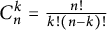 $C_n^k = \frac {n!}{k! (n-k)!}$
.
Proof All the properties are well known. For example, see [Reference Huisken and Sinestrari21] or [Reference Lieberman28] for a proof of (2.16), [Reference Li27] for (2.17), and [Reference Chou and Wang7] or [Reference Hou, Ma and Wu17] for (2.18).
The generalized Newton–MacLaurin inequality is as follows, which will be used all the time.
Proposition 2.8 For
 $\lambda \in \Gamma _k$
and
 $k> l \geq 0$
,
 $ r> s \geq 0$
,
 $k \geq r$
,
 $l \geq s$
, we have
 $$ \begin{align} \Bigg[\frac{{\sigma _k (\lambda )}/{C_n^k }}{{\sigma _l (\lambda )}/{C_n^l }}\Bigg]^{\frac{1}{k-l}} \le \Bigg[\frac{{\sigma _r (\lambda )}/{C_n^r }}{{\sigma _s (\lambda )}/{C_n^s }}\Bigg]^{\frac{1}{r-s}}. \end{align} $$
Proof See [Reference Spruck34].
3 A priori estimates
We now proceed to derive a priori estimates for solutions of equation (1.4) in this section. Equation (1.4) will be uniformly h-convex once
 $C^{2}$
estimates are established for
 $\varphi $
. By the Evans–Krylov theorem [Reference Krylov23] and Schauder theory [Reference Gilbarg and Trudinger14], one can obtain higher derivative estimates for
 $\varphi $
. Therefore, we only need to get
 $C^{2}$
estimates. For convenience, in the following of this article, we always assume that f is a smooth, positive, even function on
 $\mathbb {S}^n$
. Let M be the smooth, closed, origin-symmetric, and uniformly h-convex hypersurface in
 $\mathbb {H}^{n+1}$
with the horospherical support function
 $u=\log \varphi $
. Assume
 $\varphi $
is a smooth solution to equation (1.4). Clearly,
 $\varphi $
is a smooth, even, and uniformly h-convex solution to equation (1.4) and
 $\varphi (x)> 1$
for
 $x \in \mathbb {S}^n$
.
We will prove the following main theorem in this section.
Theorem 3.1 Let f be a smooth, even, and positive function and
 $\varphi>1$
be a smooth even h-convex solution of equation (1.4), then there is a constant
 $C>0$
depending only on n, k,
 $||f||_{C^2}$
, and
 $\min _{\mathbb {S}^n}f$
such that
 $$ \begin{align*} ||\varphi||_{C^{2}}\le C,\quad \forall x\in \mathbb{S}^{n}, \end{align*} $$
We first produce a proof of
 $C^0$
bound for
 $\varphi $
.
Lemma 3.2 We have
 $$ \begin{align} \frac{1}{2}\Big(\max_{\mathbb{S}^n}\varphi+\frac{1}{\max_{\mathbb{S}^n}\varphi}\Big)\leq \min_{\mathbb{S}^n}\varphi. \end{align} $$
Proof The inequality can be found in the proof of Lemma 7.2 in [Reference Li and Xu25]. For completeness, we give a proof here. Assume that
 $\varphi (x_1)=\max _{\mathbb {S}^n}\varphi $
and denote
 $\overline {X}(x_1)=G^{-1}(x_1)$
as before. Then, we have for any
 $x \in \mathbb {S}^n$
by the definition of the horospherical support function (2.5)
 $$ \begin{align*} -\langle \overline{X}(x_1), (x, 1)\rangle\leq \varphi(x), \quad \forall x \in \mathbb{S}^n. \end{align*} $$
Substituting the expression (2.6) for
 $\overline {X}$
into the above equality yields
 $$ \begin{align} \frac{1}{2}\varphi(x_1)(1+\langle x_1, x\rangle)+\frac{1}{2}\frac{1}{\varphi(x_1)}(1-\langle x_1, x\rangle)\leq \varphi(x), \end{align} $$
where we used the fact
 $D\varphi (x_1)=0$
. Note that
 $\varphi (x_1)\geq 1$
, we find from (3.2)
 $$ \begin{align} \frac{1}{2}\Big(\varphi(x_1)+\frac{1}{\varphi(x_1)}\Big)\leq \varphi(x) \quad \mbox{for} \quad \langle x, x_1\rangle\geq 0. \end{align} $$
Since
 $\varphi $
is even, we can assume that the minimum point
 $x_0$
of
 $\varphi (x)$
satisfies
 $\langle x_0, x_1\rangle \geq 0$
. Thus, the equality (3.1) follows that from (3.3).
Now, we use the maximum principle to get the
 $C^0$
estimate.
Lemma 3.3 Let f be a smooth, even, and positive function and
 $\varphi>1$
be a smooth, even, h-convex solution of equation (1.4). There exist constants
 $C_0>1$
depending only on the lower and upper bounds of f, k, and n such that
 $$ \begin{align} 1<C_{0}\le\varphi\leq \left ( 1+2\max_{\mathbb{S}^n }\left(\frac{f}{ C_{n}^{k} }\right)^{\frac{1}{k} }\right )^{\frac{1}{2} }+\left ( 2\max_{\mathbb{S}^n }\left(\frac{f}{ C_{n}^{k} }\right)^{\frac{1}{k} }\right )^{\frac{1}{2} }. \end{align} $$
Proof Assume the minimal value of
 $\varphi (x)$
attains at
 $x_{0}\in \mathbb {S}^n$
and choose an orthonormal local frame
 $e_{1},...,e_{n}$
near
 $x_{0}$
such that
 $(\varphi _{ij})$
is diagonal. It is obviously that
 $\left | D\varphi \right |(x_{0}) =0,~\varphi _{ii} (x_{0})\geq 0,$
and then by the definition of U,
 $U_{ii}=\varphi _{ii}+\frac {1}{2} (\varphi -\frac {1}{\varphi } )$
for any
 $1\le i\le n$
. We obtain

which leads to,
 $$ \begin{align*} f^{\frac{1}{k}} \ge \frac{1}{2}( C_{n}^{k} )^{\frac{1}{k}} \cdot (\varphi^{2}-1). \end{align*} $$
By direct calculation, we find that
 $$ \begin{align} \min_{\mathbb{S}^n } \varphi \le \left [1+ \frac{2(\max_{\mathbb{S}^n }f)^{\frac{1}{k} } }{\left ( C_{n}^{k} \right )^{^{\frac{1}{k} } } } \right ] ^{\frac{1}{2} }. \end{align} $$
From (3.1), we know,
 $$ \begin{align} ( \max_{\mathbb{S}^n }\varphi) ^{2}-( 2\min_{\mathbb{S}^n}\varphi )\max_{\mathbb{S}^n}\varphi+1\le 0, \end{align} $$
this inequality means that
 $$ \begin{align} \min_{\mathbb{S}^n}\varphi-\sqrt{(\min_{\mathbb{S}^n}\varphi)^2-1}\le\max_{\mathbb{S}^n }\varphi\le\min_{\mathbb{S}^n}\varphi+\sqrt{(\min_{\mathbb{S}^n}\varphi)^2-1}. \end{align} $$
Then, by combining (3.6) and (3.8), we derive the lower and upper bound for
 $\varphi $
,
 $$ \begin{align} \max_{\mathbb{S}^n }\varphi \le \left ( 1+2\max_{\mathbb{S}^n }\left(\frac{f}{ C_{n}^{k} }\right)^{\frac{1}{k} }\right )^{\frac{1}{2} }+\left ( 2\max_{\mathbb{S}^n }\left(\frac{f}{ C_{n}^{k} }\right)^{\frac{1}{k} }\right )^{\frac{1}{2} }. \end{align} $$
In order to obtain a exact lower bound for
 $\varphi $
, we employ the maximum principle to the maximum, following the same approach as above. Then, we have
 $$\begin{align*}\min_{\mathbb{S}^n }\varphi \ge C_{0}=\frac{1}{2}\Big(1+2\min_{\mathbb{S}^n}\left(\frac{f}{C_{n}^{k}}\right)^{\frac{1}{k}}\Big)^{\frac{1}{2}}+\frac{1}{2}\Big(1+2\min_{\mathbb{S}^n}\left(\frac{f}{C_{n}^{k}}\right)^{\frac{1}{k}}\Big)^{-\frac{1}{2}}>1.\end{align*}$$
This completes the proof of Lemma 3.3.
In order to obtain the gradient estimate, we recall Lemma 7.3 in [Reference Li and Xu25].
Lemma 3.4 For a smooth, origin symmetric, and uniformly h-convex hypersurface M in
 $\mathbb {H}^{n+1}$
, we have
 $$ \begin{align} |D \varphi|<\varphi \quad \mbox{on} \quad \mathbb{S}^n, \end{align} $$
where
 $u=log\varphi $
is the horospherical support function of M.
It is directly to see that the estimate (3.10) also holds for even, h-convex solution
 $\varphi $
of the equation (1.4), then the bound on the first derivatives immediately follows from (3.4) and (3.10).
Lemma 3.5 Let f be a smooth, even, and positive function and
 $\varphi>1$
be a smooth even h-convex solution of equation (1.4). We have
 $$ \begin{align} |D\varphi(x)|\leq C, \quad \forall \ x \in \mathbb{S}^n, \end{align} $$
where C is a positive constant depending on
 $n,k,$
and
 $\max _{\mathbb {S}^n}f$
.
Considering
 $U[\varphi ]$
is not Codazzi, in order to obtain the second derivatives estimate, we first derive following derivative exchange formula in hyperbolic space (see [Reference Chen5]), which plays a key role in our proof of
 $C^{2}$
estimates.
Lemma 3.6 For each fixed
 $x \in \mathbb {S}^n$
, we choose a local orthonormal frame so that U is diagonal at x, then, we have at x
 $$ \begin{align} U_{ij\alpha}=U_{ji \alpha}, \end{align} $$
 $$ \begin{align} U_{\alpha\alpha i}=U_{i \alpha \alpha}-\frac{\varphi_i}{\varphi}U_{ii}, \quad \alpha\neq i \end{align} $$
and
 $$ \begin{align} U_{ii\alpha\alpha}-U_{\alpha\alpha i i} & =-\frac{\sum_{k}U_{\alpha\alpha k}\varphi_k}{\varphi}-\bigg[-\frac{2\varphi_{\alpha}^{2}}{\varphi^2}+\frac{|D \varphi|^2}{2\varphi^2}+\frac{1}{\varphi}U_{\alpha\alpha}+\frac{1}{2}\Big(1+\frac{1}{\varphi^2}\Big)\bigg]U_{\alpha\alpha} \nonumber\\ &\quad +\frac{\sum_{k}U_{ii k}\varphi_k}{\varphi}+\bigg[-\frac{2\varphi_{i}^{2}}{\varphi^2}+\frac{|D \varphi|^2}{2\varphi^2}+\frac{1}{\varphi}U_{ii}+\frac{1}{2}\Big(1+\frac{1}{\varphi^2}\Big)\bigg]U_{ii}. \end{align} $$
Proof Using the Ricci identity on
 $\mathbb {S}^n$
 $$ \begin{align*} \varphi_{kji}-\varphi_{kij}=\delta_{ik}\varphi_j-\delta_{jk}\varphi_i, \end{align*} $$
we have
 $$ \begin{align*} U_{\alpha\alpha i}&= \varphi_{\alpha \alpha i}-\frac{\sum_{l}\varphi_l \varphi_{li}}{\varphi}+\frac{1}{2}\frac{|D\varphi|^2\varphi_i}{\varphi^2} +\frac{1}{2}\Big(\varphi_i+\frac{\varphi_i}{\varphi^2}\Big) \\&=\varphi_{i\alpha \alpha}-\varphi_i-\frac{\sum_{l}\varphi_l \varphi_{li}}{\varphi}+\frac{1}{2}\frac{|D\varphi|^2\varphi_i}{\varphi^2} +\frac{1}{2}\Big(\varphi_i+\frac{\varphi_i}{\varphi^2}\Big) \\&=U_{i \alpha \alpha}-\frac{\varphi_i}{\varphi}U_{ii} \end{align*} $$
and
 $$ \begin{align*} U_{ii\alpha\alpha}&=\varphi_{ii\alpha\alpha} -\frac{\sum_{k}(\varphi^{2}_{k\alpha}+\varphi_{k\alpha\alpha}\varphi_k)}{\varphi} +\frac{2\sum_{k}\varphi_{k\alpha}\varphi_k\varphi_{\alpha}}{\varphi^2}+\frac{1}{2}|D\varphi|^2 \frac{\varphi\varphi_{\alpha\alpha}-2\varphi_{\alpha}^{2}}{\varphi^3} \\ &\quad +\frac{1}{2}\Big(\varphi_{\alpha\alpha}+\frac{\varphi_{\alpha\alpha}}{\varphi^2}- \frac{2\varphi_{\alpha}^{2}}{\varphi^3}\Big) \\ &=\varphi_{ii\alpha\alpha} -\frac{\sum_{k}(\varphi^{2}_{k\alpha}+\varphi_{\alpha\alpha k}\varphi_k)}{\varphi} +\frac{\varphi_{\alpha}^{2}-|D \varphi|^2}{\varphi} +\frac{2\sum_{k}\varphi_{k\alpha}\varphi_k\varphi_{\alpha}}{\varphi^2}\\ &\quad +\frac{1}{2}|D\varphi|^2 \frac{\varphi\varphi_{\alpha\alpha}-2\varphi_{\alpha}^{2}}{\varphi^3} +\frac{1}{2}\Big(\varphi_{\alpha\alpha}+\frac{\varphi_{\alpha\alpha}}{\varphi^2}- \frac{2\varphi_{\alpha}^{2}}{\varphi^3}\Big). \end{align*} $$
Using the definition of U, it yields
 $$ \begin{align*} \frac{2\sum_{k}\varphi_{k\alpha}\varphi_k\varphi_{\alpha}}{\varphi^2}- \frac{|D\varphi|^2\varphi_{\alpha}^{2}}{\varphi^3}+\varphi_{\alpha}^{2}\Big(\frac{1}{\varphi}-\frac{1}{\varphi^3}\Big) =\frac{2\varphi_{\alpha}^{2}U_{\alpha\alpha}}{\varphi^2} \end{align*} $$
and
 $$ \begin{align*} -\frac{\sum_{k}\varphi^{2}_{k\alpha}}{\varphi}+\frac{1}{2}|D\varphi|^2 \frac{\varphi_{\alpha\alpha}}{\varphi^2} =-\frac{\varphi_{\alpha\alpha}}{\varphi}U_{\alpha\alpha}+\frac{1}{2}\varphi_{\alpha\alpha}\Big(1-\frac{1}{\varphi^2}\Big). \end{align*} $$
Thus,
 $$ \begin{align*} U_{ii\alpha\alpha}=\varphi_{ii\alpha\alpha} -\frac{\sum_{k}\varphi_{\alpha\alpha k}\varphi_k}{\varphi} -\frac{|D \varphi|^2}{\varphi} +\Big(\frac{2\varphi_{\alpha}^{2}}{\varphi^2}-\frac{\varphi_{\alpha\alpha}}{\varphi}\Big)U_{\alpha\alpha} +\varphi_{\alpha\alpha}. \end{align*} $$
Using the following Ricci identity on
 $\mathbb {S}^n$
 $$ \begin{align*} \varphi_{ii\alpha\alpha}=\varphi_{\alpha\alpha ii}-2\varphi_{\alpha\alpha}+2\varphi_{ii} \end{align*} $$
and noticing that
 $$ \begin{align*} \varphi_{\alpha\alpha k}-\varphi_{ii k}=U_{\alpha\alpha k}-U_{ii k}, \quad \varphi_{\alpha\alpha}-\varphi_{ii}=U_{\alpha\alpha}-U_{ii}, \end{align*} $$
we have
 $$ \begin{align*} &U_{ii\alpha\alpha}-U_{\alpha\alpha i i}\\&= -\frac{\sum_{k}U_{\alpha\alpha k}\varphi_k}{\varphi}+\frac{\sum_{k}U_{ii k}\varphi_k}{\varphi} +\Big(\frac{2\varphi_{\alpha}^{2}}{\varphi^2}-\frac{\varphi_{\alpha\alpha}}{\varphi}\Big)U_{\alpha\alpha} -\Big(\frac{2\varphi_{i}^{2}}{\varphi^2}-\frac{\varphi_{ii}}{\varphi}\Big)U_{ii}+U_{ii}-U_{\alpha\alpha} \\&=-\frac{\sum_{k}U_{\alpha\alpha k}\varphi_k}{\varphi}+\frac{\sum_{k}U_{ii k}\varphi_k}{\varphi} -\bigg[-\frac{2\varphi_{\alpha}^{2}}{\varphi^2}+\frac{|D \varphi|^2}{2\varphi^2}+\frac{1}{\varphi}U_{\alpha\alpha}+\frac{1}{2}\Big(1+\frac{1}{\varphi^2}\Big)\bigg]U_{\alpha\alpha} \\ &\quad +\bigg[-\frac{2\varphi_{i}^{2}}{\varphi^2}+\frac{|D \varphi|^2}{2\varphi^2}+\frac{1}{\varphi}U_{ii}+\frac{1}{2}\Big(1+\frac{1}{\varphi^2}\Big)\bigg]U_{ii}. \end{align*} $$
Lemma 3.7 If
 $tr(U)\le C $
and
 $\sigma _{2}(U)>0,$
then
 $U_{ij}\le C$
, where C is a positive constant depending on n.
Proof Notice that
 $$ \begin{align*} 0<\sigma_{2}(U)=\sum_{1\le i<j\le n}(U_{ii}U_{jj}-U_{ij}^{2})=\frac{1}{2}\left[(tr U)^{2}-\sum U_{ii}^{2}-\sum_{i\ne j}U_{ij}^{2}\right], \end{align*} $$
it follows that
 $$ \begin{align*} \sum\limits_{i=1}^nU_{ii}^{2}+\sum_{i\ne j}U_{ij}^{2}<(tr U)^{2}. \end{align*} $$
Hence, we get the desired result.
Remark For equation (1.4), when
 $k=1$
, Chen Li has already got the
 $C^2$
estimate in [Reference Chen5], so we are only going to consider the case when
 $k\ge 2.$
To complete the estimate of second derivatives, it remains to establish an upper bound for
 $tr(U)$
by Lemma 3.7.
Lemma 3.8 For
 $$ \begin{align*} U[\varphi]=D^2\varphi-\frac{1}{2}\frac{|D\varphi|^2}{\varphi}I+\frac{1}{2}\Big(\varphi-\frac{1}{\varphi}\Big)I, \end{align*} $$
we have
 $$ \begin{align*} tr(U)\le C, \end{align*} $$
where C is a positive constant depending on
 $n,k$
, and
 $\max _{\mathbb {S}^n}f$
.
Proof We now consider the auxiliary function
 $\varphi ^{n}U$
. Denote
 $F=\sigma _{k}^{\frac {1}{k}},$
thus
 $$ \begin{align} F(\lambda(U))=\sigma_{k}^{\frac{1}{k}}(\lambda(U))=\varphi^{-1}f^{\frac{1}{k}}. \end{align} $$
We may assume
 $tr(\varphi ^{n}U)$
attains its maximum at
 $x_0\in \mathbb {S}^n$
. By choosing a local orthonormal frame
 $\{e_i\}_{i=1}^n$
around
 $x_0$
such that U is diagonal, it follows that
 $\left \{F^{ij}\right \}$
and
 $U[\varphi ]$
are also diagonal at
 $x_0$
. In the following, we do the computation at
 $x_0.$
By maximum condition, we have
 $$ \begin{align} [tr(\varphi^{n}U)]_{i}=\sum_{s=1}^{n}(\varphi^{n}U_{ss})_{i}=0, \end{align} $$
 $$ \begin{align} 0\ge[tr(\varphi^{n}U)]_{ij}=\sum_{s}(\varphi^{n}U_{ss})_{ij}. \end{align} $$
Using derivative exchange formula (3.14), direct computation gives
 $$ \begin{align*} (\varphi^{n}U_{ss})_{ii}=[(\varphi^{n})_iU_{ss}+\varphi^{n}U_{ssi}]_{i}=(\varphi^{n})_{ii}U_{ss}+2(\varphi^{n})_{i}U_{ssi}+\varphi^{n}\left(U_{iiss}+A\right) \end{align*} $$
with
 $$ \begin{align*} A=&-\frac{\sum_{t}U_{ii t}\varphi_t}{\varphi}-\bigg[-\frac{2\varphi_{i}^{2}}{\varphi^2}+\frac{|D \varphi|^2}{2\varphi^2}+\frac{1}{\varphi}U_{ii}+\frac{1}{2}\Big(1+\frac{1}{\varphi^2}\Big)\bigg]U_{ii} \\&+\frac{\sum_{t}U_{ss t}\varphi_t}{\varphi}+\bigg[-\frac{2\varphi_{s}^{2}}{\varphi^2}+\frac{|D \varphi|^2}{2\varphi^2}+\frac{1}{\varphi}U_{ss}+\frac{1}{2}\Big(1+\frac{1}{\varphi^2}\Big)\bigg]U_{ss}. \end{align*} $$
Since the concavity of F and (3.17),
 $$ \begin{align} 0 &\ge \sum_{s,i=1}^{n}F^{ii}(\varphi^{n}U_{ss})_{ii} =\sum_{s,i=1}^{n}F^{ii}[(\varphi^{n})_{ii}U_{ss}+2(\varphi^{n})_{i}U_{ssi}+\varphi^{n}\left(U_{iiss}+A\right)] \nonumber\\ & =\varphi^{n}\sum_{s,i=1}^{n}F^{ii}U_{iiss}+\sum_{s,i=1}^{n}F^{ii}[(\varphi^{n})_{ii}U_{ss}+2(\varphi^{n})_{i}U_{ssi}] \nonumber\\ &\quad +\sum_{s,i=1}^{n}F^{ii}\left \{ -\frac{\varphi^{n}}{\varphi}\sum_{t}U_{ii t}\varphi_t-\varphi^{n}\bigg[-\frac{2\varphi_{i}^{2}}{\varphi^2}+\frac{|D \varphi|^2}{2\varphi^2}+\frac{1}{\varphi}U_{ii}+\frac{1}{2}\Big(1+\frac{1}{\varphi^2}\Big)\bigg]U_{ii} \right \} \nonumber\\ &\quad +\sum_{s,i=1}^{n}F^{ii}\left \{ \frac{\varphi^{n}}{\varphi}\sum_{t}U_{ss t}\varphi_t+\varphi^{n }\bigg[-\frac{2\varphi_{s }^{2}}{\varphi^2}+\frac{|D \varphi|^2}{2\varphi^2}+\frac{1}{\varphi}U_{ss}+\frac{1}{2}\Big(1+\frac{1}{\varphi^2}\Big)\bigg]U_{ss} \right \} \nonumber\\ & \triangleq F_{1}+F_{2}+F_{3}+F_{4},\nonumber\\ \end{align} $$
we will treat each term of above formula, respectively.
For the first term on the RHS of (3.18), differentiating equation (3.15) twice and by the concavity of F we have
 $$ \begin{align} F_{1}=&~\varphi^{n}[\sum_{s=1}^{n}(\varphi^{-1}f^{\frac{1}{k}})_{ss}-\sum_{s=1}^{n}F^{ij,pq}U_{ijs}U_{pqs}] \notag\\ \ge&~\varphi^{n}\sum_{s=1}^{n}\left[ (\varphi^{-1})_{ss}f^{\frac{1}{k}}+2(\varphi^{-1})_{s}(f^{\frac{1}{k}})_{s}+\varphi^{-1}(f^{\frac{1}{k}})_{ss} \right]\notag\\ \ge&-Ctr(U)-C,\ \end{align} $$
where C is a universal constant depending only on
 $\inf \varphi ,~||\varphi ||_{C^1},~\min f,~||f||_{C^2},~n,k$
. From now on, we will use C to denote universal constant depending only on
 $\inf \varphi ,~||\varphi ||_{C^1},~\min f$
,
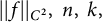 $||f||_{C^2},~n,~k,$
it may change from line to line.
We considered
 $F_{2}$
in (3.18), which is a crucial term to deal with the negative part of
 $U_{ii}^{2}$
. According to (3.16), it yields that
 $$ \begin{align} \sum_{s=1}^{n}U_{ssi}=-\varphi^{-n}\sum_{s=1}^{n}(\varphi^{m})_{i}U_{ss}, \end{align} $$
and
 $$ \begin{align} &\sum\limits_{i=1}^nF^{ii}(\varphi^{n})_{ii}\sum_{s}U_{ss}\notag \\=&\sum\limits_{i=1}^nF^{ii}\left[n(n-1)\varphi^{m-2}\varphi^{2}_{i}+n\varphi_{ii}\varphi^{n-1} \right]\big(U_{ii}+\sum_{k\neq i}U_{kk}\big) \nonumber\\=&\sum\limits_{i=1}^nF^{ii}\left[n(n-1)\varphi^{n-2}\varphi^{2}_{i}+n\varphi^{n-1}\left(U_{ii}+\frac{1}{2}\frac{|D\varphi|^{2}}{\varphi}-\frac{1}{2}(\varphi-\frac{1}{\varphi})\right) \right]\big(U_{ii}+\sum_{k\neq i}U_{kk}\big),\nonumber\\ \end{align} $$
Then, we obtain
 $$ \begin{align} F_{2}&=\sum\limits_{s,i=1}^{n}F^{ii}[(\varphi^{n})_{ii}-2\varphi^{-n}(\varphi^{n})_{i}^{2}]U_{ss}\nonumber\\ &\ge n\varphi^{n-1}\sum\limits_{i=1}^nF^{ii}U^{2}_{ii}-C\sum\limits_{i=1}^nF^{ii}tr(U). \end{align} $$
For
 $F_3$
,
 $$ \begin{align} F_{3}=&-\varphi^{n}\sum_{i,s}F^{ii}(\frac{1}{\varphi}\sum_{t}U_{iit}\varphi_{t}) -\varphi^{n}\sum_{i,s}F^{ii}\bigg[-\frac{2\varphi_{i}^{2}}{\varphi^2}+\frac{|D \varphi|^2}{2\varphi^2}+\frac{1}{\varphi}U_{ii}+\frac{1}{2}\Big(1+\frac{1}{\varphi^2}\Big)\bigg]U_{ii} \nonumber\\ =&-n\varphi^{n}\sum_{t}\frac{(\varphi^{-1}f^{\frac{1}{k}})_{t}\varphi_{t}}{\varphi}-n\varphi^{n}\sum\limits_{i=1}^{n}F^{ii}\bigg[-\frac{2\varphi_{i}^{2}}{\varphi^2}+\frac{|D \varphi|^2}{2\varphi^2}+\frac{1}{\varphi}U_{ii}+\frac{1}{2}\Big(1+\frac{1}{\varphi^2}\Big)\bigg]U_{ii} \nonumber\\ \ge&-n\varphi^{n-1}\sum\limits_{i=1}^{n}F^{ii}U_{ii}^2-C\sum\limits_{i=1}^{n}F^{ii}U_{ii}-C.\nonumber\\ \end{align} $$
Then,
 $$ \begin{align} F_{2}+F_{3}\geq -C\sum\limits_{i=1}^nF^{ii}tr(U)-C\sum\limits_{i=1}^{n}F^{ii}U_{ii}-C, \end{align} $$
As for
 $F_4$
, due to (3.20), we get
 $$ \begin{align} F_{4}&=\varphi^{n}\sum\limits_{i=1}^{n}F^{ii}[-\varphi^{-n-1}\sum_{s=1}^{n}\sum_{t=1}^n(\varphi^{n})_{t}U_{ss}\varphi_{t}] \nonumber\\ &\quad +\varphi^{n}\sum_{i,s}F^{ii}\bigg[-\frac{2\varphi_{s}^{2}}{\varphi^2}+\frac{|D \varphi|^2}{2\varphi^2}+\frac{1}{\varphi}U_{ss}+\frac{1}{2}\Big(1+\frac{1}{\varphi^2}\Big)\bigg]U_{ss} \nonumber\\ & =-\varphi^{-1}\sum\limits_{i=1}^nF^{ii}[\sum_{t}(\varphi^{n})_{t}\varphi_{t}]tr(U) \nonumber \\ &\quad +\sum_{i,s}F^{ii}\bigg[-\frac{2\varphi_{s}^{2}}{\varphi^2}+\frac{|D \varphi|^2}{2\varphi^2}+\frac{1}{\varphi}U_{ss}+\frac{1}{2}\Big(1+\frac{1}{\varphi^2}\Big)\bigg]\varphi^{n}U_{ss}\notag\\ &\ge -C\sum\limits_{i=1}^nF^{ii}tr(U)+\varphi^{n-1}\sum\limits_{i,s=1}^nF^{ii}U_{ss}^2 \end{align} $$
Plugging (3.19), (3.24), and (3.25) into (3.18), and with the aid of H
 $\ddot {o}$
lder inequality, we obtain
 $$ \begin{align} 0&\ge\sum\limits_{i,s=1}^{n}F^{ii}(\varphi^{n}U_{ss})_{ii}\notag\\ &\ge C\sum\limits_{i,s=1}^nF^{ii}U_{ss}^2-C\sum\limits_{i=1}^nF^{ii}tr(U)-Ctr(U)-C\notag\\ &\ge C\sum\limits_{i=1}^nF^{ii}tr^{2}(U)-C\sum\limits_{i=1}^nF^{ii}tr(U)-Ctr(U)-C. \end{align} $$
Meanwhile, by the Newton–Maclaurin inequality
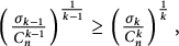 $ \left (\frac {\sigma _{k-1}}{C_{n}^{k-1}} \right )^{\frac {1}{k-1}}\ge \left (\frac {\sigma _{k}}{C_{n}^{k}} \right )^{\frac {1}{k}},$
one can get a lower bound of
 $F^{ii}$
,
 $$ \begin{align} \sum\limits_{i=1}^nF^{ii} &=\sum\limits_{i=1}^n(\sigma_{k}^{\frac{1}{k}})^{ii}=\frac{1}{k}\sigma_{k}^{\frac{1}{k}-1}\sum\limits_{i=1}^n\sigma_{k-1}(\lambda|i) \nonumber\\ &=\frac{1}{k}\sigma_{k}^{\frac{1}{k}-1}(n-k+1)\sigma_{k-1}\ge C_{n,k}. \end{align} $$
Combining (3.26) and (3.27), we can achieve
 $$ \begin{align*} tr(U)\le C, \end{align*} $$
which implies the desired result.
Combining the results in Lemmas 3.7 and 3.8, we obtain the
 $C^{2}$
estimate, which completes the proof of Theorem 3.1.
By the Evans–Krylov theorem and Schauder theory, together with the positivity of matrix
 $U[\varphi ]$
, we conclude following higher estimates.
Theorem 3.9 For each integer
 $l\geq 0$
and
 $0<\alpha <1$
, there exists a constant
 $C_{l}$
depending only on n, k, l,
 $\alpha $
,
 $||f||_{C^{l}(\mathbb {S}^{n})}$
, and
 $\min _{\mathbb {S}^{n}}f$
such that
 $$ \begin{align*} ||\varphi||_{C^{l,\alpha}}\le C_{l}, \end{align*} $$
for any even, h-convex solution
 $\varphi $
of (1.4).
4 Full rank theorem
Now we turn to the h-convexity of the solutions of equation(1.2). In this section, we will prove the following full rank theorem.
Theorem 4.1 Let f be a smooth and positive function on
 $\mathbb {S}^n$
satisfying Conditions (1) and (2) in Theorem 1.2. Let
 $\{\varphi _{i}\}_{i =1}^n$
be a sequence of smooth, even, and uniformly h-convex solutions to equation (1.4). Assuming
 $\{\varphi _{i}\}$
converges to
 $\varphi $
in
 $C^{4,\alpha }(\mathbb {S}^n)$
as
 $i \rightarrow +\infty $
. Then,
 $\varphi $
is also an even and uniformly h-convex solution to equation (1.4).
Recall
 $$ \begin{align*} U[\varphi]=D^2\varphi-\frac{1}{2}\frac{|D\varphi|^2}{\varphi}I+\frac{1}{2}(\varphi-\frac{1}{\varphi})I. \end{align*} $$
In order to prove the full rank theorem, as in [Reference Guan and Ma15], we need to establish following deformation lemma for the k-Hessian equation in hyperbolic space (1.4). The proof below follows along the lines of the proof in [Reference Guan and Ma15] by exploring some special algebraic structural properties of the Hessian operator. The proof involves some direct but lengthy computations.
For U, we rewrite (1.4) in the form
 $$ \begin{align} F\left ( U \right )=\sigma _{k}\left ( U \right )=\varphi ^{-k}f \quad \mbox{on} \quad \mathbb{S}^n, \end{align} $$
and let
 $$ \begin{align} F^{\alpha \beta}:=\frac{\partial F }{\partial W^{\alpha \beta}}, F^{\alpha \beta,\gamma s}:=\frac{\partial^{2}F}{\partial W^{\alpha \beta}{\partial W^{\gamma s}}}. \end{align} $$
We denote that
 $F^{\alpha \beta }$
is positive definite for
 $U\in \Gamma _{k}$
.
Lemma 4.2 (Deformation Lemma)
Let
 $O\subset \mathbb {S}^n$
be an open subset, suppose
 $\varphi \in C^4(O)$
is an even solution of (1.4) in O, and that the matrix U is positive semi-definite. Suppose there is a positive constant
 $C_0>0$
such that for a fixed integer
 $(n-1)\geq l\geq k\geq 2$
,
 $\sigma _l(U[\varphi (x)])\geq C_0$
for all
 $x \in O$
. Let
 $\psi (x)=\sigma _{l+1}(U[\varphi (x)])$
and let
 $\tau (x)$
be the largest eigenvalue of
 $$ \begin{align} -(f^{-\frac{1}{k}})_{ij}+|D f^{-\frac{1}{k}}|\delta_{ij} -\left(\frac{1}{\frac{8}{\left ( C_{n}^{k} \right ) ^{\frac{1}{k} }}\max_{\mathbb{S}^n}f^{\frac{1}{k}}+2}-2\right)f^{-\frac{1}{k}}\delta_{ij}. \end{align} $$
Then, there are constants
 $C_1, C_2$
depending only on
 $||\varphi ||_{C^3}$
,
 $||f||_{C^{2}}$
, n, and
 $C_0$
such that the differential inequality
 $$ \begin{align*} \sum_{\alpha,\beta}^{n}F^{\alpha\beta}(x)\psi_{\alpha\beta}(x) \le(n-l)\varphi^{-k}(x)f^{1+\frac{1}{k}}\sigma_{l}(U(x))\tau(x)+C_{1}|\bigtriangledown \psi(x)|+C_{2}\psi(x) \end{align*} $$
holds in O.
Proof The proof will follow mainly the arguments in [Reference Guan, Ma and Zhou16], which in turn were motivated by Caffarelli–Friedman [Reference Caffarelli and Friedman3] and Guan–Ma [Reference Guan and Ma15].
For any two functions defined in an open set
 $O \subset \mathbb {S}^n$
,
 $y \in O$
, we say that
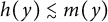 $h(y)\lesssim m(y)$
provided there exist positive constants
 $c_1$
and
 $c_2$
such that
 $$ \begin{align} h(y)-m(y)\leq c_1|\nabla \psi(y)|+c_2\psi(y). \end{align} $$
We also write
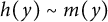 $h(y)\sim m(y)$
if
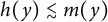 $h(y)\lesssim m(y)$
and
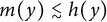 $m(y)\lesssim h(y)$
. Next, we write
 $h\lesssim m$
if the above inequality (4.4) holds in O, with the constants
 $c_1$
and
 $c_2$
depending only on
 $||\varphi ||_{C^3}$
,
 $|f|_{C^{2}}$
, n, and
 $C_0$
(independent of y and O). Finally, we write
 $h\sim m$
if
 $h\lesssim m$
and
 $m\lesssim h$
. We shall show that
 $$ \begin{align} \sum_{\alpha,\beta}^{n}F^{\alpha\beta}(x)\psi_{\alpha\beta} \lesssim (n-l)\varphi^{-k}f^{1+\frac{1}{k}}\sigma_{l}(U)\tau. \end{align} $$
For any
 $x {\kern-1pt}\in{\kern-1pt} O$
, let
 $\lambda _1{\kern-1pt}\geq{\kern-1pt} \lambda _2\geq ...\geq \lambda _n$
be the eigenvalues of U at x. Since
 ${\sigma _l(U){\kern-1pt}\geq{\kern-1pt} C_0>0}$
, there exists a positive constant
 $C>0$
such that
 $\lambda _1\geq \lambda _2\geq ...\geq \lambda _l\geq C$
. Let
 $$ \begin{align*} G=\{1, 2, ..., l\} \quad \mbox{and} \quad B=\{l+1, 2, ..., n\} \end{align*} $$
be the “good” and “bad” sets of indices, respectively. We denote by
 $\sigma _k(U|i)$
the k-th element symmetric function of U excluding the i-column and i-row and
 $\sigma _k(U|ij)$
the k-th element symmetric function of U excluding the
 $i, j$
-column and
 $i, j$
-row. Let
 $\Lambda _{G}=(\lambda _1, ..., \lambda _l)$
be the “good” eigenvalues of U at z; for convenience in notation, we also write
 $G=\Lambda _G$
if there is no confusion. In the following, all calculations are at the point x using the relation “
 $\lesssim $
”, with the understanding that the constants in (4.4) are under control.
For each fixed
 $x \in O$
, we choose a local orthonormal frame
 $e_1, ..., e_n$
so that
 $\psi $
is diagonal at x, and
 $U_{ii}=\lambda _i$
for
 $i=1, 2, ..., n$
. Now we compute
 $\psi $
and its first and second derivatives in the direction
 $e_{\alpha }$
.
As
 $\psi =\sigma _{l+1}(U)=\frac {1}{l+1}\sum _{i=1}^{n}\sigma _{l}(U|i)U_{ii}$
, we find that
 $$ \begin{align*} 0\sim \psi(z)\sim \Big(\sum_{i \in B}U_{ii}\Big)\sigma_l(G)\sim \sum_{i \in B}U_{ii}, \end{align*} $$
so
 $$ \begin{align} U_{ii}\sim 0 \quad \mbox{for all} \quad i \in B, \end{align} $$
which yields that, for
 $1\leq m\leq l$
,
 $$ \begin{align} \sigma_m(U)\sim \sigma_m(G), \quad \sigma_{m}(U|j)\sim \begin{cases} \displaystyle \sigma_{m}(G|j), & \text{if}\quad j \in G;\\[2.5ex] \displaystyle \sigma_{m}(G), & \text{if} \quad j \in B. \end{cases} \end{align} $$
 $$ \begin{align} \sigma_{m}(U|ij)\sim \begin{cases} \displaystyle \sigma_{m}(G|ij), & \text{if}\quad i, j \in G;\\[2.5ex] \displaystyle \sigma_{m}(G|j), & \text{if} \quad i \in B, j \in G;\\[2.5ex] \displaystyle \sigma_{m}(G), & \text{if} \quad i,j \in B, i\neq j. \end{cases} \end{align} $$
Moreover,
 $\psi _{\alpha }=\sigma _{l+1}^{ij}U_{ij\alpha } =\sum _{j \in B}\sigma _{l}(U|j)U_{jj\alpha }+\sum _{j \in G}\sigma _{l}(U|j)U_{jj\alpha }$
, then (4.7) tells us that
 $$ \begin{align} 0\sim \psi_{\alpha}\sim \Big(\sum_{i \in B}U_{ii\alpha}\Big)\sigma_l(G)\sim \sum_{i \in B}U_{ii\alpha}. \end{align} $$
By Proposition 2.6, we have
 $$ \begin{align} \sigma_{l+1}^{ij}\sim \begin{cases} \displaystyle \sigma_{l}(G), & \text{if}\quad i=j \in G;\\[2.5ex] \displaystyle 0, & \text{otherwise}. \end{cases} \end{align} $$
 $$ \begin{align} \sigma_{l+1}^{ij, rs}= \begin{cases} \displaystyle \sigma_{l-1}(U|ir), & \text{if}\quad i=j, r=s, i\neq r;\\[2.5ex] \displaystyle -\sigma_{l-1}(U|ij), & \text{if} \quad i\neq j, r=j, s=i;\\[2.5ex] \displaystyle 0, & \text{otherwise}. \end{cases} \end{align} $$
Since
 $$ \begin{align*} \psi_{\alpha\alpha}=\sigma_{l+1}^{ij, r s}U_{ij\alpha}U_{rs\alpha}+\sigma_{l+1}^{ij}U_{ij\alpha\alpha}, \end{align*} $$
by combining (4.11) and (3.12), it follows that for any
 $\alpha \in \{1, 2, ..., n\}$
 $$ \begin{align} \psi_{\alpha\alpha}&=\sum_{i\neq j}\sigma_{l-1}(U|i j)U_{ii\alpha}U_{jj\alpha}-\sum_{i\neq j}\sigma_{l-1}(U|i j)U^{2}_{ij\alpha}+\sum_{i=1}^{n}\sigma_{l+1}^{ii}W_{ii\alpha\alpha} \nonumber\\ &=\bigg(\sum_{i \in G, j \in B}+\sum_{i \in B, j \in G}+\sum_{i, j \in B, i\neq j}+\sum_{i, j \in G, i\neq j}\bigg)\sigma_{l-1}(U|i j)U_{ii\alpha}U_{jj\alpha}\nonumber\\ &\quad -\bigg(\sum_{i \in G, j \in B}+\sum_{i \in B, j \in G}+\sum_{i, j \in B, i\neq j}+\sum_{i, j \in G, i\neq j}\bigg)\sigma_{l-1}(U|i j)U^{2}_{ij\alpha}\nonumber\\ &\quad +\sum_{i=1}^{n}\sigma_{l+1}^{ii}U_{ii\alpha\alpha}. \end{align} $$
 $$ \begin{align} \sum_{i \in B, j \in G}\sigma_{l-1}(U|i j)U_{ii\alpha}U_{jj\alpha} \sim \bigg(\sum_{j \in G}\sigma_{l-1}(G|j)U_{jj\alpha}\bigg)\sum_{i \in B} U_{ii\alpha} \sim 0. \end{align} $$
By (4.9), for
 $\forall i\in B$
fixed and
 $\forall \alpha $
 $$ \begin{align} -U_{ii \alpha}\sim \sum_{j \in B, j\neq i}U_{jj \alpha}. \end{align} $$
 $$ \begin{align} \sum_{i, j\in B, i\neq j}\sigma_{l-1}(U|i j)U_{ii\alpha}U_{jj\alpha} \sim -\sigma_{l-1}(G)\sum_{i \in B}U^{2}_{ii\alpha}. \end{align} $$
Plugging (4.13) and (4.15) into (4.12), we obtain by (4.8)
 $$ \begin{align*} \psi_{\alpha\alpha}\sim\sum_{i=1}^{n}\sigma_{l+1}^{ii}U_{ii\alpha\alpha}-2\sum_{i \in B, j \in G}\sigma_{l-1}(G|j)U^{2}_{ij\alpha}-\sigma_{l-1}(G)\sum_{i, j \in B}U^{2}_{ij\alpha}. \end{align*} $$
So we have
 $$ \begin{align} \sum_{\alpha,\beta}F^{\alpha\beta} \psi _{\alpha\beta} &=\sum_{\alpha=1 }^{n}F^{\alpha\alpha} \psi _{\alpha\alpha} \nonumber\\ &\sim \sum_{\alpha=1}^n\sum_{i\in B}\sigma_{l+1}^{ii}F^{\alpha\alpha}U_{ii\alpha\alpha}-2\sum_{i=1}^n\sum_{i\in B,~\beta\in G}F^{\alpha\alpha}\sigma_{l-1}(G|\beta)U_{i\beta\alpha}^2\nonumber\\ &\quad -\sigma_{l-1}(G)\sum_{\alpha=1}^n\sum_{i,\beta\in B}F^{\alpha\alpha}U_{i\beta\alpha}^2. \end{align} $$
Now we compute
 $\sum _{i \in B }F^{\alpha \alpha } U_{ii\alpha \alpha }$
for
 $i \in B$
. Differentiating equation (1.4), we have
 $$ \begin{align} (\varphi^{-k}f)_{i}=\sum_{\alpha,\beta}F^{\alpha\beta}W_{\alpha\beta i},~~ (\varphi^{-k}f)_{ii}=F^{\alpha\beta,\gamma \eta }U_{\alpha\beta i}U_{\gamma\eta i}+\sum_{\alpha,\beta}F^{\alpha\beta}W_{\alpha\beta ii}. \end{align} $$
Inserting (3.14) into below equation, we obtain
 $$ \begin{align} &\sum_{i=1}^{n}\sigma_{l+1}^{ii}(U)\sum_{\alpha =1}^{n}F^{\alpha\alpha}U_{ii\alpha \alpha } \nonumber\\ &\quad =\sum_{i=1}^{n}\sigma_{l+1}^{ii}(U)\Big\{ \left ( \varphi ^{-k} f\right )_{ii}-F^{\alpha \beta ,\gamma \eta }U_{\alpha \beta i}U_{\gamma \eta i} \nonumber\\ &\qquad \left. +F^{\alpha\alpha}\left \{ -\frac{U_{\alpha\alpha k}\varphi _{k}}{\varphi}-\left [ -\frac{2\varphi^{2}_{\alpha}}{\varphi^{2} } +\frac{\left | D\varphi \right | }{2\varphi^{2}}+\frac{1}{\varphi}U_{\alpha\alpha} +\frac{1}{2}\left (\frac{1}{\varphi^{2}}+1 \right)\right]U_{\alpha\alpha}\right \} \right. \nonumber\\ &\qquad \left. +F^{\alpha\alpha}\left\{ \frac{U_{ii k}\varphi_{k}}{\varphi}+\left [ -\frac{2\varphi^{2}_{i}}{\varphi^{2} } +\frac{\left | D\varphi \right | }{2\varphi^{2}}+\frac{1}{\varphi}U_{ii} +\frac{1}{2}\left (\frac{1}{\varphi^{2}}+1 \right)\right]U_{ii}\right \} \right\} \nonumber\\ &\quad \sim \sum_{i=1}^{n}\sigma_{l+1}^{ii}(U) \Big\{ \left ( \varphi ^{-k} f\right )_{ii}-F^{\alpha \beta ,\gamma \eta }U_{\alpha \beta i}U_{\gamma \eta i} \nonumber\\ & \qquad \left.+F^{\alpha\alpha}\left\{ -\frac{U_{\alpha\alpha k}\varphi _{k}}{\varphi}-\left [ -\frac{2\varphi^{2}_{\alpha}}{\varphi^{2} } +\frac{\left | D\varphi \right | }{2\varphi^{2}}+\frac{1}{\varphi}U_{\alpha\alpha} +\frac{1}{2}\left (\frac{1}{\varphi^{2}}+1 \right)\right]U_{\alpha\alpha}\right \} \right\}, \end{align} $$
where we used below facts in the last relation:
 $$ \begin{align*} \sum_{i=1}^{n}\sigma_{l+1}^{ii}(U)U_{ii}\sim \psi \sim 0, \end{align*} $$
and
 $$ \begin{align*} \sum_{i=1}^{n}\sigma_{l+1}^{ii}(U)U_{iik}=\psi_{k}\sim 0. \end{align*} $$
Similar to the proof method in Euclidean space, we group the second term on the RHS of equation (4.18) as:
 $$ \begin{align} & \quad -F^{\alpha \beta ,\gamma \eta }U_{\alpha \beta i}U_{\gamma \eta i} =-\sum_{\alpha \ne \beta}\sigma_{k-2} (U\mid\alpha\beta)U_{\alpha\alpha i}U_{\beta\beta i}+\sum_{\alpha \ne \beta}\sigma_{k-2}(U\mid \alpha\beta)U_{\alpha\beta i}^{2} \nonumber\\& =-\left(2\sum_{\alpha \in B,\beta \in G}+\sum_{\alpha,\beta \in G, \alpha \ne \beta}+\sum_{\alpha,\beta \in B,\alpha \ne \beta}\right)\sigma_{k-2}(U\mid \alpha\beta)U_{\alpha\alpha i}U_{\beta\beta i} \nonumber \\[3pt]&\quad +\sum_{\alpha \ne \beta}\sigma_{k-2}(U \mid \alpha\beta)U_{\alpha\beta i}^{2} \nonumber\\[3pt]& \sim -\sum_{\alpha,\beta \in G,\alpha \ne \beta}\sigma_{k-2}(U\mid\alpha\beta)U_{\alpha\alpha i}U_{\beta\beta i}-\sum_{\alpha,\beta \in B,\alpha \ne \beta}\sigma_{k-2}(U\mid\alpha\beta)U_{\alpha\alpha i}U_{\beta\beta i} \nonumber\\[3pt]&\quad +\sum_{\alpha \ne \beta}\sigma_{k-2}(U \mid \alpha\beta)U_{\alpha\beta i}^{2}, \end{align} $$
here we have used again
 $\sum _{i \in B}U_{ii\alpha } \sim 0$
.
Plugging (4.17) and (4.19) into (4.18), we get for any
 $i\in B,$
 $$ \begin{align} &F^{\alpha\alpha}\psi_{\alpha\alpha} \nonumber \\[2pt]&\quad =\frac{-(n-l)\sigma_{l}(G)\sum_{j=1}^{n}(\varphi ^{-k}f)_{j}\varphi_{j}}{\varphi}\nonumber\\&\quad -\sum_{i\in B}\sigma_{l}(G)\sum _{\alpha=1}^{n}\sigma_{k-1}(U\mid\alpha) \nonumber\left[ \frac{-2\varphi_{\alpha}^{2}}{\varphi^{2}}+\frac{\left | D\varphi \right |^{2} }{2\varphi^{2}}+\frac{1}{\varphi}U_{\alpha\alpha}+\frac{1}{2} (1+\frac{1}{\varphi^{2}})\right]U_{\alpha\alpha}\notag\\[4pt]&\quad +\sigma_{l}(G)\sum_{i\in B}(\varphi^{-k}f)_{ii}-\sigma_{l}(G)\sum_{i\in B}\sum_{\alpha,\beta\in G,\alpha\ne\beta}\sigma_{k-2}(G\mid\alpha\beta)U_{\alpha\alpha i}U_{\beta\beta i}\notag\\&\quad -\sigma_{l}(G)\sum_{i\in B}\sum_{\alpha,\beta\in B,\alpha \ne\beta}\sigma_{k-2}(G)U_{\alpha\alpha i}U_{\beta\beta i} +\sigma_{l}(G) \sum_{i\in B}\sum_{\alpha,\beta=1,\alpha\ne\beta}^{n}\sigma_{k-2}(U\mid\alpha\beta)U_{\alpha\beta i}^{2}\nonumber\\&\quad -2\sum_{\alpha=1}^{n}\sum_{i\in B,~\beta\in G}\sigma_{l-1}(G\mid \beta)\sigma_{k-1}(U\mid\alpha)U_{i\beta\alpha}^{2}-\sum_{\alpha=1}^{n}\sigma_{l-1}(G)\sum_{i,\beta\in B}\sigma_{k-1}(U\mid\alpha)U_{i\beta\alpha}^{2} \nonumber\\[3pt]&\quad\triangleq (1)+(2)+(3)+(4)+(5)+(6)+(7)+(8).\nonumber\\ \end{align} $$
The terms in (4.20) need to be further simplified. We first settle the second term of(4.20). Noticing that
 $|B|=n-l$
, so
 $\sum _{i\in B}\sum _{\alpha =1}^{n}\sigma _{k-1}(|\alpha )U_{\alpha \alpha }=(n-l)k\sigma _{k}$
. Recalling the
 $C^{1}$
estimate in the previous section
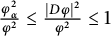 $\frac {\varphi _{\alpha }^{2}}{\varphi ^{2}}\le \frac {\left | D\varphi \right |^{2}}{\varphi ^{2}}\le 1$
, we have
 $$ \begin{align} (2)\sim(n-l)k\sigma_{l}(G)\varphi^{-k}f\left(\frac{\left | D\varphi \right |^{2}}{\varphi^{2}}-\frac{1}{2\varphi^{2}}\right). \end{align} $$
Next we deal with the sixth and seventh terms on the RHS of (4.20). For the sixth term,
 $$ \begin{align*} & \sum_{\alpha\ne\beta}\sigma_{l}(G) \sigma_{k-2}(U\mid\alpha\beta)U_{\alpha\beta i}^{2}\\ &\quad =\left[ 2\sum_{\alpha\in B,\beta\in G}+\sum_{\alpha,\beta\in G,\alpha\ne\beta}+\sum_{\alpha,\beta\in B,\alpha\ne\beta}\right]\sigma_{l}(G) \sigma_{k-2}(U\mid\alpha\beta)U_{\alpha\beta i}^{2} \nonumber\\ &\quad \triangleq (6.1)+(6.2)+(6.3), \end{align*} $$
and for the seventh term,
 $$ \begin{align*} & -2\sum_{\alpha=1}^{n}\sum_{\beta\in G}\sigma_{l-1}(G\mid \beta)\sigma_{k-1}(U\mid\alpha)U_{i\beta\alpha}^{2} \\ &\quad =\left[-2\sum_{\alpha\in B,\beta \in G}-2\sum_{\alpha,\beta\in G,\alpha\ne\beta}-2\sum_{\alpha,\beta\in B,\alpha=\beta} \right]\sigma_{k-1}(U\mid\alpha)U_{i\beta\alpha}^{2} \nonumber\\ & \quad \triangleq (7.1)+(7.2)+(7.3) \end{align*} $$
We are devoted to show that
 $$ \begin{align} (6.1)+(7.1) & \sim ~2\sum_{i\in B}\sum_{\alpha\in B,\beta\in G}\sigma_{l}(G)\sigma_{k-2}(G\mid\alpha\beta)U_{\alpha\beta i}^{2} \nonumber\\ &\quad -2\sum_{i\in B}\sum_{\alpha\in B,\beta\in G}\sigma_{l-1}(G\mid \beta)\sigma_{k-1}(U\mid\alpha)U_{i\beta\alpha}^{2} \nonumber\\ & \lesssim ~0. \end{align} $$
Indeed, we know for any
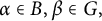 $\alpha \in B,\beta \in G,$
 $$\begin{align*}\sigma_{l}(G)\sigma_{k-2}(U|\alpha\beta)\sim\sigma_{l-1}(G| \beta)U_{\beta\beta}\sigma_{k-2}(G|\beta)\lesssim\sigma_{l-1}(G| \beta)\sigma_{k-1}(G),\end{align*}$$
and it is easy to check that
 $U_{\alpha \beta i}=U_{i\beta \alpha } $
for
 $ i\in B,\alpha \in B, \beta \in G$
on the standard
 $\mathbb {S}^{n}$
(recall the Ricci identity
 $\varphi _{\alpha \beta i}=\varphi _{i\beta \alpha }+\delta _{i\alpha }\varphi _{\beta }-\delta _{\beta \alpha }\varphi _{i}$
). So (4.22) follows. Noticing that
 $$ \begin{align*} (7.2)\sim&-2\sum_{i\in B}\sum_{\alpha,\beta\in G,\alpha\ne\beta}\sigma_{l-1}(G\mid \beta)\sigma_{k-1}(G\mid\alpha)U_{i\beta\alpha}^{2} \nonumber\\ \lesssim&-2\sum_{i\in B}\sum_{\alpha,\beta\in G,\alpha\ne\beta}\sigma_{l-1}(G\mid \beta)U_{\beta\beta}\sigma_{k-2}(G\mid\alpha\beta)U_{i\beta\alpha}^{2} \nonumber\\ \sim&-2\sum_{i\in B}\sum_{\alpha,\beta\in G,\alpha\ne\beta}\sigma_{l}(G)\sigma_{k-2}(G\mid\alpha\beta)U_{i\beta\alpha}^{2}, \end{align*} $$
by using
 $U_{i\beta \alpha }=U_{\alpha \beta i}$
for
 $i\in B,~ \alpha ,\beta \in G,$
and
 $\alpha \ne \beta $
again, we observe that
 $$ \begin{align} (6.2)+(7.2)\lesssim 0. \end{align} $$
From (4.22) and (4.23), we conclude that
 $$ \begin{align} (6)+(7) & \lesssim (6.3)+(7.3) \sim \sum_{i\in B}\sum_{\alpha,\beta\in B,\alpha\ne\beta}\sigma_{l}(G)\sigma_{k-2}(U\mid\alpha\beta)U_{\alpha\beta i}^{2} \nonumber\\ &\quad -2\sum_{i\in B}\sum_{\alpha\in G}\sigma_{l-1}(G\mid \alpha)\sigma_{k-1}(G\mid\alpha)U_{\alpha\alpha i}^{2}, \end{align} $$
where we used (3.13) in the last relation. Plugging (4.21) and (4.24) into (4.20), we obtain
 $$ \begin{align} F^{\alpha\alpha}\psi_{\alpha\alpha} &\lesssim \frac{-(n-l)\sigma_{l}(G)\sum_{j=1}^{n}(\varphi ^{-k}f)_{j}\varphi_{j}}{\varphi}+\sigma_{l}(G)\sum_{i\in B}(\varphi^{-k}f)_{ii} \nonumber\\ &\quad +(n-l)k\sigma_{l}(G)\varphi^{-k}f \left(\frac{\left | D\varphi \right |^{2}}{\varphi^{2}}-\frac{1}{2\varphi^{2}}\right) \nonumber\\ &\quad -\left(1+\frac{1}{k}\right)\sum_{i\in B}\frac{(\varphi^{-k}f)_{i}^{2}}{\varphi^{-k}f}\sigma_{l}(G)+I_{1}+I_{2}+I_{3}, \end{align} $$
where
 $$ \begin{align*} I_{1}=&\sum_{i\in B}\sum_{\alpha,\beta\in B,\alpha\ne\beta}\sigma_{l}(G) \sigma_{k-2}(G\mid\alpha\beta)U_{\alpha\beta i}^{2}-\sigma_{l}(G) \sum_{i\in B}\sum_{\alpha,\beta\in B,\alpha \ne\beta}\sigma_{k-2}(G)U_{\alpha\alpha i}U_{\beta\beta i} \nonumber\\ &-\sum_{i=1}^{n}\sigma_{l-1}(G)\sum_{\alpha,\beta\in B}\sigma_{k-1}(U\mid i)U_{\alpha\beta i}^{2}, \end{align*} $$
 $$ \begin{align*} I_{2}&=-\sum_{i\in B}\sum_{\alpha\in G}\sigma_{l-1}(G\mid\alpha)\sigma_{k-1}(G\mid\alpha)U_{\alpha\alpha i}^{2} \\ &\quad -\sigma_{l}(G) \sum_{i\in B}\sum_{\alpha,\beta\in G,\alpha\ne\beta}\sigma_{k-2}(G\mid\alpha\beta)U_{\alpha\alpha i}U_{\beta\beta i} +\sum_{i\in B}\frac{(\varphi^{-k}f)^{2}_{i}}{\varphi^{-k}f}\sigma_{l}(G), \end{align*} $$
and
 $$ \begin{align*} I_{3}=-\sum_{i\in B}\sum_{\alpha\in G}\sigma_{l-1}(G\mid\alpha)\sigma_{k-1}(G\mid\alpha)U_{\alpha\alpha i}^{2}+\frac{1}{k}\sum_{i\in B}\frac{(\varphi^{-k}f)^{2}_{i}}{\varphi^{-k}f}\sigma_{l}(G). \end{align*} $$
Claim 1.
 $I_{1}\lesssim 0,I_{2}\lesssim 0$
, and
 $I_{3}\lesssim 0.$
In fact, since
 $$ \begin{align*} \sum_{\alpha,\beta\in B,\alpha \ne\beta}U_{\alpha\alpha i}U_{\beta\beta i}\sim\sum_{\alpha\in B}U_{\alpha\alpha i}(\sum_{\beta\ne\alpha}U_{\beta\beta i})\sim-\sum_{\alpha\in B}U_{\alpha\alpha i}^{2}, \end{align*} $$
and
 $$ \begin{align*} -\sum_{i=1}^{n}\sigma_{l-1}(G)\sum_{\alpha,\beta\in B}\sigma_{k-1}(U\mid i)U_{\alpha\beta i}^{2} =&-\sum_{i=1}^{n}\sigma_{l-1}(G)\sum_{\alpha,\beta\in B}\sigma_{k-1}(U\mid i)U_{\alpha\beta i}^{2} \\ \lesssim&-\sigma_{l-1}(G)\sigma_{k-1}(G)\sum_{i \in B}\sum_{\alpha,\beta\in B}U_{\alpha\beta i}^{2}, \end{align*} $$
then for any
 $i\in B,$
we have
 $$ \begin{align} I_{1}\lesssim&\sum_{i\in B}\sum_{\alpha,\beta\in B,\alpha\ne\beta}\sigma_{l}(G) \sigma_{k-2}(G\mid\alpha\beta)U_{\alpha\beta i}^{2}+\sum_{i\in B}\sum_{\alpha\in B}\sigma_{l}(G)\sigma_{k-2}(G)U_{\alpha\alpha i}^{2} \nonumber\\ &-\sigma_{l-1}(G)\sigma_{k-1}(G)\sum_{i \in B}\sum_{\alpha,\beta\in B}U_{\alpha\beta i}^{2} \nonumber\\ \lesssim& \left[\sigma_{l}(G)\sigma_{k-2}(G)-\sigma_{l-1}(G)\sigma_{k-1}(G)\right]\sum_{\alpha,\beta\in B}U_{\alpha\beta i}^{2} \nonumber\\ \lesssim& 0, \end{align} $$
where we used the Newton–Maclaurin inequality in the last inequality.
To treat
 $I_{2}$
, by using Lemma 2.3 in [Reference Guan and Ma15], direct calculation yields that
 $$ \begin{align*} (\varphi^{-k}f)I_{2} & \sim \Big[-\sum_{i\in B}\sum_{\alpha\in G}\sigma_{l-1}(G\mid\alpha)\sigma_{k-1}(G\mid\alpha)U_{\alpha\alpha i}^{2}\\ &\quad -\sigma_{l}(G)\sum_{i\in B}\sum_{\alpha,\beta\in G,\alpha\ne\beta}\sigma_{k-2}(G\mid\alpha\beta)U_{\alpha\alpha i}U_{\beta\beta i}\Big]\sigma_{k}(G)\\ &\quad +\sum_{i\in B}\Big[\sum_{\alpha\in G}\sigma_{k-1}(G\mid\alpha)U_{\alpha\alpha i}\Big]^{2}\sigma_{l}(G)\\ &\sim \sum_{i\in B}\Bigg \{\sum_{\alpha\in G}\Big[\sigma_{l}(G) \sigma_{k-1}^{2}(G\mid\alpha)-\sigma_{l-1}(G\mid\alpha)\sigma_{k-1}(G\mid\alpha)\sigma_{k}(G)\Big] U_{\alpha\alpha i}^{2}\\ &\quad +\sum_{\alpha,\beta\in G,\alpha\ne\beta}\Big[ \sigma_{l}(G)\sigma_{k-2}(G\mid\alpha)\sigma_{k-1}(G\mid\beta) \\ &\quad -\sigma_{l}(G)\sigma_{k-2}(G\mid\alpha\beta)\sigma_{k}(G) \Big]U_{\alpha\alpha i}U_{\beta\beta i}\Bigg \} \\ &\lesssim 0, \end{align*} $$
it means that
 $I_{2}\lesssim 0.$
Now we deal with
 $I_{3}$
.
 $$ \begin{align} I_{3}\sim&\frac{1}{k(\varphi^{-k}f)}\sum_{i\in B}\left[\sum_{\alpha\in G}\sigma_{l}(G)^{\frac{1}{2}}\sigma_{k-1}(G|\alpha)U_{\alpha\alpha i} \right] ^{2}-\sum_{i\in B}\sum_{\alpha\in G}\sigma_{l-1}(G\mid\alpha)\sigma_{k-1}(G\mid\alpha)U_{\alpha\alpha i}^{2} \nonumber\\ =&\sum_{i\in B}\left\{\frac{1}{k(\varphi^{-k}f)}\left[\sum_{\alpha\in G} \left(\sigma_{l-1}^{\frac{1}{2}}(G|\alpha)\sigma_{k-1}^{\frac{1}{2}}(G|\alpha)U_{\alpha\alpha i} \right) \left(\sigma_{k-1}^{\frac{1}{2}}(G|\alpha)U_{\alpha\alpha}^{\frac{1}{2}} \right) \right]^{2} \right. \nonumber\\&-\left.\sum_{\alpha\in G}\sigma_{l-1}(G\mid\alpha)\sigma_{k-1}(G\mid\alpha)U_{\alpha\alpha i}^{2} \right\} \nonumber\\ \lesssim&\sum_{i\in B}\left\{\frac{1}{k(\varphi^{-k}f)}\left[\sum_{\alpha\in G} \sigma_{l-1}(G|\alpha)\sigma_{k-1}(G|\alpha)U_{\alpha\alpha i}^{2} \sum_{\beta\in G} \sigma_{k-1}(G|\beta)U_{\beta\beta} \right] \right. \nonumber\\&-\left.\sum_{\alpha\in G}\sigma_{l-1}(G\mid\alpha)\sigma_{k-1}(G\mid\alpha)U_{\alpha\alpha i}^{2} \right\} \sim 0.\nonumber\\ \end{align} $$
Then, Claim 1 is verified. (4.25) turns to
 $$ \begin{align} F^{\alpha\alpha}\psi_{\alpha\alpha} \nonumber\lesssim&\frac{-(n-l)\sigma_{l}(G)\sum_{j=1}^{n}(\varphi ^{-k}f)_{j}\varphi_{j}}{\varphi}+\sigma_{l}(G)\sum_{i\in B}(\varphi^{-k}f)_{ii} \nonumber\\&+(n-l)k\sigma_{l}(G)\varphi^{-k}f(\frac{\left | D\varphi \right |^{2}}{\varphi^{2}}-\frac{1}{2\varphi^{2}})-(1+\frac{1}{k})\sum_{i\in B}\frac{(\varphi^{-k}f)_{i}^{2}}{\varphi^{-k}f}\sigma_{l}(G). \end{align} $$
Direct calculation yields
 $$ \begin{align} -(1+\frac{1}{k})\sum_{i\in B}\frac{(\varphi^{-k}f)_{i}^{2}}{\varphi^{-k}f} =&-\frac{1+k}{k}(-k\varphi^{-k-1}\varphi_{i}f+\varphi^{-k}f_{i})^{2}\varphi^{k}f^{-1} \nonumber\\ =&-\frac{1+k}{k}(k^{2}\varphi^{-2k-2}\varphi_{i}^{2}f^{2}-2k\varphi^{-2k-1}\varphi_{i}f_{i}f+\varphi^{-2k}f_{i}^{2})\varphi^{k}f^{-1} \nonumber\\ =&-k(k+1)\varphi^{-k}\frac{\varphi_{i}^{2}}{\varphi^{2}}f+2(1+k)\varphi^{-k}\frac{\varphi_{i}}{\varphi}f_{i}-\frac{1+k}{k}\varphi^{-k}\frac{f_{i}^{2}}{f}, \end{align} $$
and
 $$ \begin{align} (\varphi^{-k}f)_{ii}&=(-k\varphi^{-k-1}\varphi_{i}f+\varphi^{-k}f_{i})_{i} \nonumber\\&= k(k+1)\varphi^{-k-2}\varphi_{i}^{2}f-k\varphi^{-k-1}\varphi_{ii}f-2k\varphi^{-k-1}\varphi_{i}f_{i}+\varphi^{-k}f_{ii} \nonumber\\&\sim k(1+k)\varphi^{-k}\frac{\varphi_{i}^{2}}{\varphi^{2}}f-\frac{k}{2}\varphi^{-k}f\frac{\left | D\varphi \right |^{2}}{\varphi^{2}} \nonumber\\&\quad +\frac{k}{2}\varphi^{-k}f \left(1-\frac{1}{\varphi^{2}} \right)-2k\varphi^{-k}\frac{\varphi_{i}f_{i}}{\varphi} +\varphi^{-k}f_{ii}, \end{align} $$
where we used the fact that for any
 $i\in B$
,
$$ \begin{align*} 0 \sim U_{ii}=\varphi_{ii}-\frac{1}{2}\frac{|D\varphi|^2}{\varphi}+\frac{1}{2}\Big(\varphi-\frac{1}{\varphi}\Big), \end{align*} $$
and
 $$ \begin{align} \frac{-\sum^{n}_{j=1}(\varphi^{-k}f)_{j}\varphi_{j}}{\varphi} &=\frac{-\sum^{n}_{j=1}(-k\varphi^{-k-1}\varphi_{j}f+\varphi^{-k}f_{j})\varphi_{j}}{\varphi} \notag\\&=k\varphi^{-k}f\frac{| D\varphi |^{2}}{\varphi^{2}}-\sum_{j=1}^{n}\varphi^{-k}\frac{f_{j}\varphi_{j}}{\varphi}. \end{align} $$
Combining (4.29)–1(4.31), we can get
 $$ \begin{align} \sum F^{\alpha\beta}\psi_{\alpha\beta}&\lesssim\varphi^{-k}\sigma_{l}(G)\sum_{i\in B}\big[f_{ii}+(2k+2-2k)\frac{\varphi_{i}f_{i}}{\varphi}-\sum_{j=1}^{n}\frac{\varphi_{j}f_{j}}{\varphi}+\frac{3}{2}kf\frac{\left| D\varphi \right|{}^{2}}{\varphi^{2}} \\& \quad +\frac{k}{2}(1-2\frac{1}{\varphi^{2}})-\frac{1+k}{k}\frac{f_{i}^{2}}{f}\big] \nonumber\\&=\varphi^{-k}\sigma_{l}(G)\sum_{i\in B}\big[f_{ii}+2\frac{\varphi_{i}f_{i}}{\varphi}-\sum_{j=1}^{n}\frac{\varphi_{j}f_{j}}{\varphi}+2kf-k\frac{f}{\varphi^{2}}-\frac{1+k}{k}\frac{f_{i}^{2}}{f}\big].\notag \end{align} $$
Set
 $$ \begin{align*} B=2\sum_{i\in B}\frac{\varphi_{i}f_{i}}{\varphi}-\sum_{i\in B}\sum_{j=1}^{n}\frac{\varphi_{j}f_{j}}{\varphi}. \end{align*} $$
Claim 2.
 $B\le \sum _{i\in B}|Df|$
.
According to the direct calculation of
 $(f^{-\frac {1}{k}})_{i}$
and
 $(f^{-\frac {1}{k}})_{ii}$
, we obtain that
 $$ \begin{align} |Df|=kf^{\frac{1}{k}+1}|Df^{-\frac{1}{k}}|, \end{align} $$
and
 $$ \begin{align} f_{ii}=(1+\frac{1}{k})\frac{f_{i}^{2}}{f}-k(f^{-\frac{1}{k}})_{ii}f^{\frac{1}{k}+1}. \end{align} $$
If the claim is true, it follows from(4.32)–(4.34) that
 $$ \begin{align} \sum F^{\alpha\beta}\psi_{\alpha\beta} &\le\varphi^{-k}\sigma_{l}(G)\sum_{i\in B}[f_{ii}+|Df|-\frac{1+k}{k}\frac{f_{i}^{2}}{f}+kf(2-\frac{1}{\varphi^{2}})] \nonumber\\&=k\varphi^{-k}f^{1+\frac{1}{k}}\sigma_{l}(G)\sum_{i\in B}[-(f^{-\frac{1}{k}}_{ii})+|Df^{-\frac{1}{k}}|+(2-\varphi^{2})f^{-\frac{1}{k}}]. \end{align} $$
Moreover, by the
 $C^{0}$
estimate(3.4), we conclude that
 $$ \begin{align} & \sum F^{\alpha\beta}\psi_{\alpha\beta} \nonumber \\ & \quad \le k\varphi^{-k}f^{1+\frac{1}{k}}\sigma_{l}(G)\sum_{i\in B}\left \{ -(f^{-\frac{1}{k}}_{ii})+|Df^{-\frac{1}{k}}|+\left [ 2-\frac{1}{\frac{8}{(C_{n}^{k})^\frac{1}{k}}maxf^{\frac{1}{k}}+2}\right ] f^{-\frac{1}{k}}\right \} . \end{align} $$
Thus the lemma follows from (4.36).
Proof of Claim 2
Case 1: If
 $\sum _{\beta \in B}\varphi _{\beta }f_{\beta }> 0,$
thus
 $$ \begin{align*} B&\le\sum_{i\in B}\left(2\sum_{\beta\in B}\frac{\varphi_{\beta}f_{\beta}}{\varphi}-\sum_{j=1}^{n}\frac{\varphi_{j}f_{j}}{\varphi}\right) =\sum_{i\in B}\left(2\sum_{\beta\in B}\frac{\varphi_{\beta}f_{\beta}}{\varphi}-\sum_{\alpha\in G}\frac{\varphi_{\alpha}f_{\alpha}}{\varphi}\right) \\&\le\sum_{i\in B}\sum_{i=1}^{n}\frac{|\varphi_{i}f_{i}|}{\varphi} \le\frac{\left(\sum\limits_{i=1}^n\varphi_{i}^{2}\right)^{\frac{1}{2}}\left(\sum\limits_{i=1}^nf_{i}^{2}\right)^{\frac{1}{2}}}{\varphi} \\&\le |Df|. \end{align*} $$
Case 2: If
 $\sum _{\beta \in B}\varphi _{\beta }f_{\beta }< 0,$
thus
 $$ \begin{align*} B\le-\sum_{i\in B}\frac{\left \langle Df,D\varphi \right \rangle }{\varphi} \le \sum_{i\in B}\frac{|Df||D\varphi|}{\varphi} \le \sum_{i\in B}|Df|. \end{align*} $$
Claim 2 is verified. Then, the proof of the Deformation Lemma is complete.
Now we begin to prove Theorem 4.1.
Proof If
 $\varphi $
is not uniformly h-convex, there exists an integer l with
 $l \ge k$
such that
 $\sigma _{l}(U[\varphi ])\ge 0$
for any
 $x\in \mathbb {S}^{n}$
and
 $\psi (x_{0})=\sigma _{l+1}(U[\varphi (x_{x}])=0 $
for some
 $x_{0} \in \mathbb {S}^{n}$
. Using Lemma 4.2, we have
 $$ \begin{align*} \sum_{\alpha,\beta}^{n}F^{\alpha\beta}(x)\psi_{\alpha\beta}(x) \le C_{1}|\bigtriangledown \psi(x)|+C_{2}\psi(x). \end{align*} $$
The strong minimum principle implies
 $\psi =\sigma _{l+1}(U[\varphi ])\equiv 0.$
Then, we have
 $\varphi \equiv 1$
by using (2.9). This is a contradiction to (1.4).
5 Existence via degree theory
The main object of this section is to establish an existence result for equation (1.4). With the priori estimates established in the previous section, one may wish to apply the continuity method to get the existence. Unfortunately, while the closeness follows from the estimates, the openness is difficult to establish due to the lack of geometric obstructions. Instead, we will approach the problem using degree theory (see [Reference Li26]), which leads to the study of linearized operator L of the Hessian operator in (1.4).
In order to compute the degree, we need the uniqueness of constant solutions to equation(1.4).
Lemma 5.1 Let
 $\gamma $
be a positive constant, then, the h-convex solutions to equation
 $$ \begin{align} \sigma_{k}(U)=\varphi^{-k}\gamma \end{align} $$
with
 $\varphi>1$
are given by
 $$ \begin{align*} \varphi(x)=\Big[1+2\left(\frac{\gamma}{C_{n}^{k}}\right)^{\frac{1}{k}}\Big]^{\frac{1}{2}}\Big(\sqrt{|x_0|^2+1}-\langle x_0, x\rangle\Big), \end{align*} $$
where
 $x_0 \in \mathbb {R}^{n+1}$
. In particular,
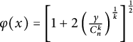 $\varphi (x)=\left [1+2\left (\frac {\gamma }{C_{n}^{k}}\right )^{\frac {1}{k}}\right ]^{\frac {1}{2}}$
is the unique even solution.
Proof When
 $k=1$
, this lemma can be easily deduced by Obata’s theorem [Reference Obata31] (see also Theorem B.2 in Appendix B in [Reference Gidas and Spruck13]). For any
 $1<k\leq n$
, this lemma is a corollary of Proposition 8.1 in [Reference Li and Xu25], its proof is simil ar to that of Theorem 8.1 (7).
We set
 $$ \begin{align*} \mathcal{B}^{2,\alpha}(\mathbb{S}^n)=\{\varphi \in C^{2,\alpha}(\mathbb{S}^n): \varphi \ \mbox{is even}\} \end{align*} $$
and
 $$ \begin{align*} \mathcal{B}_{0}^{4,\alpha}(\mathbb{S}^n)=\{\varphi \in C^{4,\alpha}(\mathbb{S}^n): U[\varphi]>0 \ \mbox{and} \ \varphi \ \mbox{is even}\}. \end{align*} $$
For
 $0\le t\le 1,$
we define
 $$\begin{align*}\mathcal{L}(\varphi, t)=\sigma_{k}(U)-\varphi^{-k} f_t,\end{align*}$$
where
 $f_t=[(1-t)(\max _{\mathbb {S}^n}f)^{-\frac {1}{k}}+t f^{-\frac {1}{k}}]^{-k}$
, then for each fixed
 $\varphi $
,
 is a differential operator that maps
 $\mathcal {B}_{0}^{4,\alpha }(\mathbb {S}^n)$
into
 $\mathcal {B}^{2,\alpha }(\mathbb {S}^n)$
. It is easy to check that
 $f_{t}$
satisfies the conditions in full rank theorem (Theorem 4.1),
 $\varphi _{t}$
is uniformly h-convex, then according to a priori estimates in previous sections (Theorems 3.3, 3.5, and 3.1), if R is sufficiently large, there exists no solution of
 $\mathcal {L}(\varphi , t)=0$
on the boundary of
 $$\begin{align*}\mathcal{O}_R=\{\varphi \in \mathcal{B}_{0}^{4,\alpha}(\mathbb{S}^n): 1+\frac{1}{R}< \varphi, \ 0< U[\varphi], \ ||\varphi||_{C^{4,\alpha}(\mathbb{S}^n)}<R\},\end{align*}$$
which clearly is an open set of
 $\mathcal {B}_{0}^{4,\alpha }(\mathbb {S}^n)$
. Consequently, the degree
 is well-defined for
 $0\leq t\leq 1$
. Since degree is a homotopic invariant ( [Reference Li26, Proposition 2.2]), we have

According to Lemma 5.1,
 $\varphi =c$
is the unique even solution for
 $\mathcal {L}(\varphi , 0)=0$
in
 $\mathcal {O}_R$
. We may compute the degree using the formula
 $\deg (L_{c_0}, \mathcal {O}_R, 0)=\sum _{\lambda _{j}>0}(-1)^{\beta _{j}},$
where
 $\lambda _{j}$
are the eigenvalues of the linearized operator of
 $\mathcal {L}$
and
 $\beta _{j}$
is its multiplicity. Direct calculation shows that the linearized operator of
 $\mathcal {L}$
at
 $\varphi =c$
is
 $$ \begin{align*} L_{c}(\overline{\phi})=\left[\frac{1}{2}\left(c-\frac{1}{c}\right)\right]^{k-1} C_{n-1}^{k-1}(\Delta_{\mathbb{S}^n}+n)\overline{\phi}. \end{align*} $$
Since
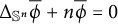 $\Delta _{\mathbb {S}^n}\overline {\phi }+n\overline {\phi }=0$
has the unique even solution
 $\overline {\phi }=0$
,
 $L_{c}$
is an invertible operator. So, we have by Proposition 2.3 in [Reference Li26]
 $$ \begin{align*} \deg(\mathcal{L}(\cdot, 0), \mathcal{O}_R, 0)=\deg(L_{c_0}, \mathcal{O}_R, 0). \end{align*} $$
Because the eigenvalues of the Beltrami–Laplace operator
 $\Delta $
on
 $\mathbb {S}^n$
are strictly less than
 $-n$
except for the first two eigenvalues
 $0$
and
 $-n$
, there is only one positive eigenvalue with multiplicity
 $1$
, which is
 $n{\cdot}\left [\frac {1}{2}\left (c-\frac {1}{c}\right )\right ]^{k-1} C_{n-1}^{k-1}$
. Then, we have by Proposition 2.4 in [Reference Li26]
 $$ \begin{align*} \deg(\mathcal{L}(\cdot, 0), \mathcal{O}_R, 0)=\deg(L_{c_0}, \mathcal{O}_R, 0)=- 1. \end{align*} $$
Therefore, it follows from (5.2)
 $$ \begin{align*} \deg(\mathcal{L}(\cdot, 1), \mathcal{O}_R; 0)=\deg(\mathcal{L}(\cdot, 0), \mathcal{O}_R, 0)=- 1. \end{align*} $$
So, we obtain a solution at
 $t=1$
. This completes the proof of Theorem 1.2.



