


Impact Statement
This research paper discusses a method for uncertainty quantification via ensemble generation for training an end-to-end data assimilation (DA) model under the 4DVarNet framework and UNet. To this end, this paper describes a novel method for ensemble generation for spatiotemporal data in the context of geosciences. It demonstrates the approach to two neural network models, 4DVarNet and UNet, that are trained for reconstruction tasks in training and shows the utility in producing ensemble outputs for uncertainty quantification. Its primary goal is to show how such structural choices that are inspired by the problem domain at hand are not only better at hidden state estimation problems but also pave the way for uncertainty quantification. The broader community may find this desirable for application and research in DA and geosciences.
1. Introduction
In geosciences, deep learning (DL) has emerged as a new way of approaching state reconstruction and forecasting problems. Through a training phase, deep neural architectures capture complex nonlinear relationships within a vast amount of spatiotemporal data (LeCun et al., Reference LeCun, Bengio and Hinton2015). By contrast, traditional physically based methods rely on data assimilation (DA) frameworks (Trémolet, Reference Trémolet2007; Carrassi et al., Reference Carrassi, Bocquet, Bertino and Evensen2018). They explicitly leverage physical knowledge, but they are often computationally expensive for multiple runs. They also generally rely on simplified models and assumptions to remain tractable (Blum et al., Reference Blum, Le Dimet and Navon2009; Asch et al., Reference Asch, Bocquet and Nodet2016; Bannister, Reference Bannister2017; Carrassi et al., Reference Carrassi, Bocquet, Bertino and Evensen2018).
The DA community has also witnessed a continuously evolving landscape of model architectures for developing applications with a focus on improving different components and algorithms in the DA pipeline (Cheng et al., Reference Cheng, Quilodrán-Casas, Ouala, Farchi, Liu, Tandeo, Fablet, Lucor, Iooss, Brajard, Xiao, Janjic, Ding, Guo, Carrassi, Bocquet and Arcucci2023). End-to-end neural architectures tailored to the structural knowledge of the underlying DA problem have seen new architectural discoveries and refinement of those suited best to the task (Fablet et al., Reference Fablet, Chapron, Drumetz, Mémin, Pannekoucke and Rousseau2021; Beauchamp et al., Reference Beauchamp, Febvre, Georgenthum and Fablet2023a; Farchi et al., Reference Farchi, Chrust, Bocquet, Laloyaux and Bonavita2023; Martin et al., Reference Martin, Manucharyan and Klein2025).
However, the application of DL in DA is not without challenges: a critical challenge lies in uncertainty quantification and the model’s generalization ability to unseen data. It is thus important to obtain both the best estimate and to quantify the associated uncertainty in DA (van Leeuwen et al., Reference van Leeuwen, Chiu and Yang2025). Ensemble methods in particular have been the cornerstone of physics-based operational DA systems (Palmer and Zanna, Reference Palmer and Zanna2013; Carrassi et al., Reference Carrassi, Bocquet, Bertino and Evensen2018). They rely on stochastic perturbation of physical parameters and perturbed initial conditions that are used to initialize the model (Palmer and Zanna, Reference Palmer and Zanna2013; Bannister, Reference Bannister2017). In DL, modern methods have gained importance to generate new states from noise, such as probabilistic diffusion models (Ho et al., Reference Ho, Jain and Abbeel2020). Their ability to sample physically consistent states in inverse problem setting remain a scientific challenge (Cheng et al., Reference Cheng, Quilodrán-Casas, Ouala, Farchi, Liu, Tandeo, Fablet, Lucor, Iooss, Brajard, Xiao, Janjic, Ding, Guo, Carrassi, Bocquet and Arcucci2023; Martin et al., Reference Martin, Manucharyan and Klein2025).
Here, we investigate how to embed uncertainty quantification in end-to-end neural DA schemes, namely 4DVarNets introduced by Fablet et al. (Reference Fablet, Chapron, Drumetz, Mémin, Pannekoucke and Rousseau2021). Leveraging physically consistent random perturbation schemes, we introduce a novel ensemble neural DA scheme, 4DVarNet-LU, extending 4DVarNets (Fablet et al., Reference Fablet, Chapron, Drumetz, Mémin, Pannekoucke and Rousseau2021) to uncertainty quantification issues. The considered random perturbations model location-based uncertainties through spatiotemporal coherent displacements in physical space using Gaussian random fields. We demonstrate that training with an initial state that reflects both prior knowledge and positional error can be used to obtain an ensemble of reconstructions from a given set of partial observations at inference. We exploit the approach to explore how such schemes could help in reducing reconstruction biases and uncertainties of DA systems. We report for one-layer quasi-geostrophic dynamics (Frezat et al., Reference Frezat, Le Sommer, Fablet, Balarac and Lguensat2022) with sparse observations, seen as an intermediate-complexity testbed representation of sea surface dynamics (Le Guillou et al., Reference Le Guillou, Gaultier, Ballarotta, Metref, Ubelmann, Cosme and Rio2023). Our results support the relevance of the end-to-end neural DA to enhance ensemble reconstruction when dealing with partially observed systems.
2. Methodology
We briefly introduce the problem of variational DA that we focus on in this work, called the weak-4DVar. This is the most general form of variational DA since the underlying physical model is rarely perfect (Trémolet, Reference Trémolet2007; Fletcher, Reference Fletcher and Fletcher2017). The objective here is to find the state sequence over a time window, denoted by
$ {X}^i=\left\{{x}_1,{x}_2,..,{x}_n\right\} $
 that fits the sparse and noisy observations
$ {Y}^i=\left\{{y}_1,{y}_2,\dots {y}_n\right\} $
 over a time window
$ {t}_1:{t}_n $
 observed on some domain
$ \Omega =\left\{{\Omega}_1,{\Omega}_2,..,{\Omega}_n\right\} $
 . This translates to an inverse problem solved by the minimization of the weak-constraint 4DVar cost
$ \mathcal{J} $
 , given by

While Equation (2.1) is minimized, it is computationally expensive for large-scale optimization using adjoint computations. The computational complexity obviously increases to ensemble DA with such model-based variational schemes.
End-to-end trainable DL methods present an alternative approach for such inverse problems in space–time dynamical systems. It reformulates the inverse problem as learning a neural operator
$ {\Psi}_{\theta } $
 to predict the target state
$ {X}^t $
 directly from observations and partial state information. This results in the optimization problem (2.2):

While generic architectures such as UNets can be used for this purpose, recent work has shown that embedding variational DA principles within neural architectures improves physical consistency and generalization (Fablet et al., Reference Fablet, Chapron, Drumetz, Mémin, Pannekoucke and Rousseau2021; Beauchamp et al., Reference Beauchamp, Febvre, Georgenthum and Fablet2023a). Building on this perspective, we now introduce the two end-to-end DL models that we use in this work.
2.1. 4DVarNet
4DVarNet is an end-to-end, data-driven neural network approach that learns both the 4DVar variational cost and its solver together (Fablet et al., Reference Fablet, Chapron, Drumetz, Mémin, Pannekoucke and Rousseau2021). It has a neural-network-parameterized 4DVar cost as part of the architecture given by

where the first term contains the observation operator
$ H $
 and measures the misfit between the estimated state
$ X $
 and the observations
$ Y $
 . The second term is a regularization term
$ \lambda \parallel X-\Phi (X)\parallel $
 , which is an autoencoder that can be interpreted as a learned representation for the state sequence in a low-dimensional manifold. A trainable, long short-term memory (LSTM)-based gradient-based solver is used to minimize this cost iteratively as

The end-to-end training of 4DVarNet leads to a bi-level optimization problem (Da Li et al., Reference Da Li, Song and Hospedales2018; Schwartz et al., Reference Schwartz, Giryes and Bronstein2019). The objective is to solve the inner minimization problem, which is achieved by minimizing the reconstruction performance criterion defined in Equation (2.2) during training.
2.2. 4DVarNet-LU: position-based uncertainty via coherent random displacements
In DA literature, it is known that the quality of initial prior state information is reflected in the quality of reconstruction for the unknown state (Carrassi et al., Reference Carrassi, Bocquet, Bertino and Evensen2018). Hence, we propose the modified 4DVarNet architecture to output the reconstructed state by taking both the initial guess and the observations
$ \left({X}^0,Y\right) $
 as input to predict the true state
$ X $
 , which we refer to as 4DVarNet-LU, which we describe in Section 2.2. It differs from the standard 4DVarNet (Fablet et al., Reference Fablet, Chapron, Drumetz, Mémin, Pannekoucke and Rousseau2021; Beauchamp et al., Reference Beauchamp, Febvre, Georgenthum and Fablet2023a) where the state
$ {X}^0 $
 is initialized directly from the sparse observations. A conceptual overview of the modified architecture is illustrated in Figure 1, where the initial state estimate
$ {X}^0 $
 is obtained by randomly sampling states around the true state via coherent displacements in position.
Schematic of 4DVarNet-LU showing the adaptation of original architecture (Fablet et al., Reference Fablet, Chapron, Drumetz, Mémin, Pannekoucke and Rousseau2021) to include an initialization method based on a random coherent displacement model.

Figure 1. Long description
The flowchart is organized into three main sections from left to right.
1. Input Section (Left):
* Top: A stack of satellite-like track maps labeled Obs, represented by the variable Y.
* Bottom: A stack of heatmaps labeled Initial State, represented by the variable X super 0. Below this are two equations: X super 0 (x vector, t) equals X (x vector plus S super i (x vector, t), t) and S super i (x vector, t) is distributed as G R F (sigma sub disp, L, T).
2. Iterative Processing Block (Center):
* Enclosed in a dashed rounded rectangle labeled Repeat block n equals 1 to K.
* Variable Y enters a blue box labeled U sub Phi.
* Variable X super 0 enters the block and becomes X super n minus 1 in the feedback loop.
* U sub Phi connects via an arrow labeled A D to a box containing Nabla sub x U sub Phi.
* This gradient box points down into a larger blue box labeled L S T M sub Gamma (Nabla sub x U).
* The output of the L S T M passes through a summation circle, becoming X super n, which feeds back to the start of the block and also exits to the right.
3. Output Section (Right):
* The final state X super K points to a stack of smooth heatmaps labeled reconstruction.
* At the bottom right, a legend defines Phi as Auto-encoder.
Position-based errors are well known in operational DA, where dynamically consistent structures (e.g., eddies or vortices) may be correctly represented but displaced in space and/or time. Such misalignment errors lead to the well-known double-penalty issue in DA (Lawson and Hansen, Reference Lawson and Hansen2005; Nehrkorn et al., Reference Nehrkorn, Woods, Hoffman and Auligné2015; Bocquet et al., Reference Bocquet, Vanderbecken, Farchi, Le Brazidec and Roustan2024).
Motivated by this, we propose a method to generate an ensemble of initial states by coherently perturbing a reference state, tailored to reconstruction problems in DA. To preserve physical consistency over the assimilation window, the induced errors are required to be both spatially and temporally correlated. This motivates the use of a Gaussian random field to sample a coherent displacement field, in contrast to diffusion-based probabilistic approaches (Ho et al., Reference Ho, Jain and Abbeel2020), which rely on unstructured random noise that is subsequently mapped to physical space.
To generate a new perturbed state
$ {X}^{ptb} $
 from the true state
$ X $
 , we sample a coherent random displacement field
$ {S}^i(\overrightarrow{x},t) $
 from a GRF, denoted by
$ \mathcal{G}\mathcal{RF}\left({\sigma}_{disp},L,\mathcal{T}\right) $
 and use it to displace the field
$ X $
 in space and time, given by

The parameter
$ {\sigma}_{disp} $
 controls the standard deviation of the field.
$ L $
 and
$ \mathcal{T} $
 are the spatial and temporal correlation lengths, and together control the spatiotemporal consistency of
$ {S}^i(\overrightarrow{x},t) $
 across the DA window. An illustrative figure of the stream function field is shown in Figure 2. As the displacement is spatially nonuniform, the mean displacement magnitude at any position
$ \overrightarrow{x} $
 is given by

The top row illustrates the true stream function field. The second row shows the perturbed stream function field obtained using the coherent random perturbations with
$ L=5.0,\mathcal{T}=20.0 $
 , and
$ {\sigma}_{disp}=7.0 $
 . The contour lines show iso-curves at five levels.

Figure 2. Long description
A two-by-five grid of heat maps.
* Vertical Color Scale: Located on the right, ranging from negative 6 (dark red) to positive 6 (dark blue), representing the stream function values.
* Top Row (True field X): Five panels showing the evolution of fluid flow at days 1, 3, 5, 7, and 9. Each panel features a prominent dark red cyclonic region in the upper right and a dark blue anticyclonic region in the lower left. White dashed and solid contour lines indicate five iso-curve levels.
* Bottom Row (X super p t b): Five panels showing the perturbed field at the same time intervals. While the general dipole structure of red and blue regions remains similar to the top row, the shapes of the high-intensity cores and the positioning of the white contour lines show stochastic variations and slight spatial shifts compared to the true field.
* Axes: Each panel is bounded by a y-axis from 0 to 120 and an x-axis from 0 to 125.
We refer to the obtained state
$ {X}^{ptb}(\overrightarrow{x},t) $
 as a perturbed state corresponding to the true state
$ X(\overrightarrow{x},t) $
 . For a given observation sequence
$ Y $
 , Equation (2.5) enables sampling different initial state realizations
$ {X}^0 $
 from the true target state
$ X $
 to train 4DVarNet-LU. In training, we sample
$ {\sigma}_{disp} $
 from a uniform distribution
$ \mathcal{U}\left(0,{\sigma}_{max}\right) $
 so that the model learns to adapt to the quality of the initial state. As in traditional ensemble DA, this approach generates the ensemble by running the models with multiple initial states independently with the same set of observations, rather than from stochasticity in the model parameters or training procedure. More details about the training and inference configurations can be found in the Supplementary Material.
2.3. UNet
We now briefly describe the UNet architecture that is used in this work. We use a standard convolutional UNet (Ronneberger et al., Reference Ronneberger, Fischer, Brox, Navab, Hornegger, Wells and Frangi2015) as a feed-forward baseline to provide a direct mapping from observations
$ Y $
 to the target stream function
$ X $
 , each of shape
$ \left[T,H,W\right] $
 . Next, we modify the input for UNet where we concatenate
$ \left(Y,{X}^{ptb}\right) $
 along the channel dimension. The architecture follows an encoder–decoder structure with skip connections and produces a single output tensor of shape
$ \left[T,H,W\right] $
 . This model is trained end-to-end in the same training configuration, training data, and loss function as 4DVarNet-LU. This UNet performs a single-pass feed-forward prediction and does not incorporate an explicit variational formulation or iterative solver structure.
3. Result
Performance is evaluated in an observation system simulation experiment (OSSE) framework based on a single-layer quasi-geostrophic model with periodic boundary conditions on a
$ 128\times 128 $
 grid. Sparse observations are generated by applying a pseudo-nadir altimetry track mask to the stream function fields. An example of the inputs, reconstructions, and reference states is shown in Figure 3. We present results for 4DVarNet-LU and UNet using identical training and testing configurations, where the training is restricted to sample
$ {\sigma}_{disp}\sim \mathcal{U}\left(0,{\sigma}_{max}\right) $
 ,
$ {\sigma}_{max}=15.0 $
 , and tested systematically for different levels of perturbations
$ {\sigma}_{disp} $
 . This value of
$ {\sigma}_{max} $
 is chosen empirically to be commensurate with the radius of the eddy features, thereby constraining perturbations to a physically plausible range of spatial variability in this system.
The first row shows the true stream function
$ X $
 for 7 consecutive days in the test period of 81 days, starting from day 20. The second row displays the sparse pseudo-nadir altimetry tracks as observations
$ Y $
 . The third and fourth are the 4DVarNet-LU and UNet mean obtained from ensemble of size 25, respectively.

Figure 3. Long description
The visualization consists of 28 panels arranged in four rows and seven columns.
* The first row, labeled Ground Truth, shows continuous heatmaps of the stream function X. Blue regions indicate positive values concentrated in the upper-left and upper-right, while red regions indicate negative values in the lower-center. White contour lines delineate the intensity gradients.
* The second row, labeled Observations, shows sparse pseudo-nadir altimetry tracks as diagonal, dotted lines of color against a white background. These represent the limited data points available for Y.
* The third row, labeled 4 D Var Net L U, displays the mean reconstruction from an ensemble of 25. The heatmaps closely mirror the Ground Truth row, showing smooth transitions and accurate placement of the blue and red vortices.
* The fourth row, labeled U Net, shows the mean reconstruction from a U Net ensemble of 25. While similar to the ground truth, the features appear slightly more diffused compared to the 4 D Var Net L U results.
At the bottom, a horizontal color bar titled Stream function Value maps the data from negative 4 in dark red to 0 in white, and up to positive 4 in dark blue.
We first consider an unbiased ensemble, obtained by sampling the first-guess state at inference around
$ {X}^t $
 , followed by a biased initial ensemble, where a biased state
$ {X}^{bias} $
 is constructed from the true state and ensemble members are sampled around
$ {X}^{bias} $
 for different values of
$ {\sigma}_{disp} $
 . Reconstruction quality is assessed using
$ RMSEs $
 score of ensemble mean reconstruction
$ \hat{X}(t) $
 over the test period of
$ 81 $
 days. We compute its mean
$ \mu $
 and standard deviation
$ \sigma \left[ RMSEs(t)\right] $
 , where

To evaluate the ensembles, we use the spatially averaged continuous ranked probability score (CRPS), which penalizes both bias and overconfidence in the ensemble (Hersbach, Reference Hersbach2000). For an ensemble of size
$ N $
 with members
$ {\left\{{x}_j\right\}}_{j=1}^N $
 and reference truth (or analysis)
$ {x}^t $
 , the CRPS is defined as

Importantly, we evaluate the model beyond
$ {\sigma}_{max} $
 at test time to assess its ability to generalize to more extreme perturbations. At inference, each ensemble member is conditioned on an independent observation noise realization, analogous to the perturbed-observation approach in the ensemble Kalman filter (EnKF) (Burgers et al., Reference Burgers, van Leeuwen and Evensen1998). Notably, we also consider the cases where both 4DVarNet and UNet models are trained directly on observations to the ground truth.
3.1. Reducing reconstruction uncertainties from a first guess
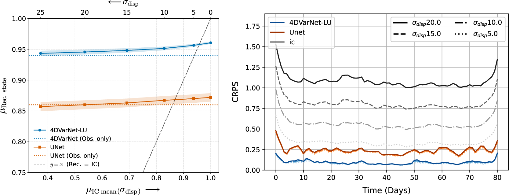
To illustrate the mean state from 4DVarNet-LU & UNet, we plot the mean reconstruction of 25 ensemble members in Figure 3. From the left panel of Figure 4, we see that even if individual initial conditions are away from the true state, the ensemble mean obtained from these models learn to correctly reduce the errors beyond those seen in training, notably
$ {\sigma}_{ptb}=20,25 $
 . Here, the spread represents the standard deviation
$ \sigma \left[ RMSEs(t)\right] $
 of the ensemble mean over the test period. We also notice a threshold for both models as
$ {\sigma}_{disp} $
 approaches
$ 0 $
 , where location errors smaller than this do not gain improvement. For UNet, this threshold is between
$ {\sigma}_{disp}=5\;\mathrm{and}\;{\sigma}_{disp}=10.0 $
 , whereas for 4DVarNet-LU it is observed below
$ {\sigma}_{disp}=5.0 $
 .
Ensemble mean performance
$ \mu $
 for 4DVarNet-LU and UNet as a function of test-time perturbation amplitude
$ {\sigma}_{\mathrm{disp}} $
 . The plot highlights the robustness of 4DVarNet and UNet to increasing perturbations in the initial state.

Figure 4. Long description
The figure consists of two panels.
Left Panel: A line graph showing mu sub Rec. state on the y-axis (ranging from 0.75 to 1.00) versus mu sub I C mean (sigma sub disp) on the x-axis (ranging from 0.4 to 1.0). A secondary top x-axis shows sigma sub disp decreasing from 25 to 0.
* 4 D Var Net L U (blue line with circles) shows a slight positive linear trend from 0.94 to 0.96.
* U Net (orange line with squares) shows a slight positive linear trend from 0.86 to 0.87.
* Horizontal dotted lines represent ‘Obs. only’ baselines for both models.
* A dashed diagonal line represents y equals x (Rec. equals I C).
Right Panel: A line graph showing C R P S on the y-axis (ranging from 0.00 to 1.75) versus Time in Days on the x-axis (ranging from 0 to 80).
* The top black line (i c) represents the highest error, fluctuating around 1.1.
* Three grey dashed/dotted lines represent sigma sub disp values of 20.0, 15.0, and 10.0, showing decreasing error levels.
* The U Net (orange line) and 4 D Var Net L U (blue line) are at the bottom, with 4 D Var Net L U maintaining the lowest C R P S near 0.1 throughout the 80-day period.
While 4DVarNet-LU consistently performs better than UNet at all perturbation levels, both models show similar trend: we see that their reconstruction scores are fairly stable with a slight but gradual decrease in the accuracy for higher displacement levels
$ {\sigma}_{\mathrm{disp}} $
 , indicating the impact of error in the initial guess. This behavior is expected since, given a sequence of observations, a better initial condition should need less correction.
The second panel for CRPS in Figure 4 shows the temporal structure of CRPS, which also complements the stability of the ensemble for both models. The CRPS value is not affected by the level of perturbation, although it degrades by a very small amount, which is not visible in the plot. For the exact value of these details, we include a separate tables in the Supplementary Material for both metrics. Figure 11 in the Supplementary Material illustrates the visual difference across the ensemble for reconstruction.
3.2. Biased DA ensemble as first guess: out-of-distribution generalization
To assess the robustness of this approach outside the training distribution, we look at the performance of both 4DVarNet-LU and UNet when the initial ensemble mean is biased. We introduce it by imposing a constant spatially coherent displacement on the true state consistent across all assimilation windows, yielding the average positional shift value
$ b $
 . Figure 5 shows the ensemble mean performance over the
$ \left({\sigma}_{\mathrm{disp}},b\right) $
 in parameter space. We see a gradual decrease in performance for both models, highlighting the joint sensitivity to initial ensemble bias and spread. We observe that the performance is highest for zero bias in the initial ensemble. Whereas if the initial ensemble is biased, there is a gradual decline in the reconstruction performance. This expected behavior points to the fact that training was entirely in the unbiased initial state scenarios. Further increases in bias magnitude result in limited additional degradation, indicating the impact of observations compensating for the error in the initial condition.
Mean performance
$ \mu $
 over the ensemble bias and ensemble spread parameter space for 4DVarNet-LU (left) and UNet (right).

Figure 5. Long description
A two-panel heatmap display. Both panels share a common X-axis labeled sigma sub disp with an arrow pointing right, ranging from 0 to 25, and a Y-axis labeled Bias with an arrow pointing up, ranging from 0.00 to 28.28.
Left Panel: Titled 4 D Var Net L U. The color scale for mu ranges from 0.90 (dark purple) to 0.95 (yellow). The highest performance is concentrated in the bottom row where Bias is 0.00, showing a bright yellow band across all sigma sub disp values. As Bias increases, performance drops sharply into a uniform dark purple region across the rest of the parameter space.
Right Panel: Titled U Net. The color scale for mu ranges from 0.845 (dark blue) to 0.870 (yellow). This panel shows a diagonal gradient. The highest performance (yellow) is at the bottom-left corner (Bias 0, sigma sub disp 0). Performance decreases as both Bias and sigma sub disp increase, with the lowest values (dark blue) located in the top-right corner. Unlike the left panel, the transition is gradual across both axes.
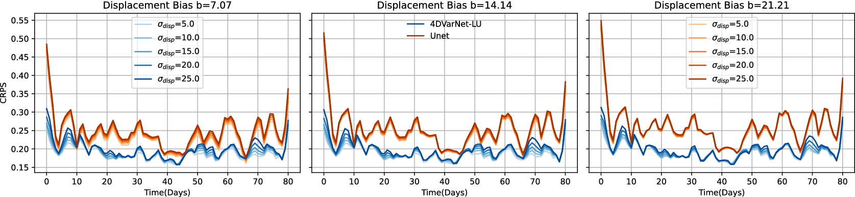
Figure 6 shows the spatially averaged CRPS for 4DVarNet-LU and UNet as a function of time for different levels of biased initial ensemble. While 4DVarNet-LU is better than UNet, for any fixed bias, both show a gradual increase in CRPS with increasing
$ {\sigma}_{\mathrm{disp}} $
 . Here, we observe that the displacement bias in the initial ensemble mean has more pronounced effect, while the ensemble spread around this biased mean does not necessarily compensate for the bias (Figures 7 and 8). While smaller
$ {\sigma}_{\mathrm{disp}} $
 ensembles achieve slightly lower CRPS, it has limited impact on the overall score, suggesting that the temporal trend is largely dominated by the bias component of CRPS (Figure 6).
Continuous ranked probability score (CRPS) as a function of time, averaged over spatial dimensions. Lower values indicate improved probabilistic performance.

Figure 6. Long description
A three-panel line graph with a shared Y-axis labeled C R P S ranging from 0.15 to 0.55 and a shared X-axis labeled Time in Days ranging from 0 to 80.
* The left panel is titled Displacement Bias b equals 7.07. It shows a series of blue lines representing 4 D Var Net L U with sigma sub disp values from 5.0 to 25.0 and an orange line for Unet. Both models start with a high C R P S near 0.50 at day 0, dropping sharply. The blue lines fluctuate between 0.15 and 0.25, while the orange line remains higher, fluctuating between 0.20 and 0.30.
* The center panel is titled Displacement Bias b equals 14.14. The legend identifies the blue lines as 4 D Var Net L U and the orange line as Unet. The performance gap widens slightly compared to the first panel, with the orange Unet line showing more pronounced peaks near 0.30.
* The right panel is titled Displacement Bias b equals 21.21. It includes a legend for sigma sub disp values from 5.0 to 25.0. The blue 4 D Var Net L U lines remain relatively stable in the 0.15 to 0.25 range, while the orange Unet line shows the highest C R P S values of the three panels, frequently peaking above 0.30.
In all panels, the blue lines representing 4 D Var Net L U consistently maintain a lower C R P S than the orange Unet line, indicating better probabilistic performance.
Error for different ensemble members for bias = 7.07, day = 50,
$ {\sigma}_{disp}=15.0 $
 .

Figure 7. Long description
A series of six square heatmaps arranged horizontally, each representing a different realization of error.
* The panels are titled from left to right as Realization 0 Error, Realization 1 Error, Realization 2 Error, Realization 3 Error, Realization 4 Error, and Realization 5 Error.
* Each heatmap displays a complex, organic pattern of red and blue regions. Red areas indicate negative error values, while blue areas indicate positive error values.
* The patterns are similar across all six panels but show slight variations in the shape and intensity of the peaks and troughs. Generally, there are prominent red clusters in the bottom-left and bottom-right quadrants, and smaller red and blue patches scattered in the upper half.
* Dashed contour lines delineate specific intensity thresholds within the colored regions.
* On the far right, a vertical color scale bar titled Error Value provides the legend. The scale ranges from negative 0.75 at the bottom in dark red, through white at 0.00, to positive 0.75 at the top in dark blue.
Although CRPS is known to favor increased uncertainty for biased Gaussian forecasts, the ensemble in this case (Figure 7) represents coherent, non-Gaussian uncertainties associated with structural and position errors (Lawson and Hansen, Reference Lawson and Hansen2005; Nehrkorn et al., Reference Nehrkorn, Woods, Hoffman and Auligné2015). As a result, increasing the positional displacement
$ {\sigma}_{disp} $
 does not necessarily improve reliability and instead leads to higher CRPS (Figure 6).
Temporal behavior of the ensemble over the test period chosen at two different spatial locations for 4DVarNet-LU and UNet. The displacement bias is given by
$ b=21.21 $
 and
$ {\sigma}_{\mathrm{disp}}=10.0 $
 . The solid lines denote the ensemble mean, and the shaded regions indicate 95% confidence intervals computed using the Student-t distribution for an ensemble of size
$ n=25 $
 .

Figure 8. Long description
A multi-panel line graph with two vertically stacked plots. Both plots share an x-axis labeled Time with an arrow pointing right, ranging from 0 to 80, and a y-axis labeled Stream function value.
Top Panel (x=64, y=64):
- The y-axis ranges from -4 to 4.
- A black line represents True Data, showing a fluctuating trend starting near 1, dipping to -2 at time 10, and rising to nearly 2 by time 50.
- A blue line (4 D Var Net L U Mean) and an orange line (U Net Mean) closely track the black True Data line throughout the period.
- A green line (Initial Ensemble Mean) shows a smoother, less accurate approximation of the True Data.
- Shaded regions indicate 95 percent confidence intervals: light green for Initial Ensemble (widest), light blue for 4 D Var Net L U (narrowest), and light orange for U Net.
Bottom Panel (x=10, y=10):
- The y-axis ranges from -4 to 3.
- The black True Data line shows higher volatility, with a significant drop to nearly -4 at time 52.
- The blue 4 D Var Net L U Mean and orange U Net Mean lines remain highly synchronized with the True Data, capturing the sharp troughs and peaks.
- The green Initial Ensemble Mean fails to capture the depth of the troughs after time 40, remaining significantly higher than the True Data.
- The confidence intervals follow the same color coding as the top panel, with the Initial Ensemble again showing the highest uncertainty (widest shaded area).
4. Conclusions
DA methods combine observations with some prior estimate or background knowledge to solve inverse problems. We explore how initial conditions information could be used in neural DA methods, by primarily focusing on two DL models that can be trained to solve the DA task, 4DVarNet-LU and UNet. Using the ideas of position-based uncertainty in DA, we propose a method to systematically sample states around a given true state in a controllable manner using coherent random displacements in physical space. The proposed strategy provides a physically plausible mechanism to generate structured variability using a Gaussian random field model that preserves continuity and enforces spatiotemporal coherence, a key characteristic of physically realistic fields. The proposed scheme becomes a part of the new learning strategy where it preserves the large-scale coherent structures while generating randomness for ensemble generation. During inference, the trained model can be used to obtain an ensemble of reconstructions when used with an ensemble of initial conditions for the same set of observations. Our experiments on a quasi-geostrophic model show that 4DVarNet-LU consistently outperforms UNet as quantified by RMSE and CRPS metrics. The performance gap between 4DVarNet-LU and UNet can be attributed to the former’s DA-based variational-formulation-aware architecture (Fablet et al., Reference Fablet, Chapron, Drumetz, Mémin, Pannekoucke and Rousseau2021; Beauchamp et al., Reference Beauchamp, Febvre, Georgenthum and Fablet2023a). Importantly, even for biased initial ensembles not seen during training, 4DVarNet-LU maintains superior reconstruction skill over UNet, demonstrating good skill in correcting the bias in reconstruction to some level and generalization beyond the training distribution. While global quantities such as mass or mean field value remain preserved under our proposed scheme, local gradients and fine-scale structures may be modified due to interpolation, and further study of the effects on conservation of higher-order derived quantities such as energy and vorticity is required. This work is a step toward robust methods and strategies for understanding and further developing uncertainty-aware DL-based neural DA models.
Supplementary material
The supplementary material for this article can be found at http://doi.org/10.1017/eds.2026.10058.
Acknowledgments
The authors acknowledge the computing resources provided by IMT Atlantique for access to the Odyssey server, which were used for model training and inference in this work.
Author contribution
Conceptualization: S.K.R., R.F.; Data curation: S.K.R.; Formal analysis: S.K.R.; Funding acquisition: R.F.; Investigation: S.K.R.; Methodology: S.K.R., R.F.; Software: S.K.R.; Supervision: R.F.; Visualization: S.K.R.; Writing—original draft: S.K.R.; Writing—review and editing: S.K.R., R.F.
Competing interest
The authors declare that they have no known competing financial interests or personal relationships that could have appeared to influence the work reported in this paper.
Data availability statement
The simulation data used in this study are publicly available on Zenodo, which contains quasi-geostrophic stream function and vorticity ground truth fields, as well as satellite-track observations of the stream function (doi:10.5281/zenodo.16890868). All the model code, training configuration, inference scripts, and figure reproduction scripts are available at https://github.com/Mr-Markovian/4DVarNet-LU.
Ethics statement
The research meets all ethical guidelines, including adherence to the legal requirements of the study country.
Funding statement
This work was supported by the European Union’s Horizon Europe research and innovation programme under grant agreement No. 101137682 (AI4PEX—Artificial Intelligence and Machine Learning for Enhanced Representation of Processes and Extremes in Earth System Models; doi:/10.3030/101137682).
Provenance statement
This article is part of the Climate Informatics 2026 proceedings and was accepted in Environmental Data Science on the basis of the Climate Informatics peer review process.






 Open access

