An inverse problem for the space–time fractional Schrödinger equation on closed manifolds

Li Li

doi:10.4153/S0008439526102124

An inverse problem for the space–time fractional Schrödinger equation on closed manifolds

Part of: Miscellaneous topics - Partial differential equations

Published online by Cambridge University Press: 04 June 2026

Li Li

Show author details

Li Li*: Affiliation:
Tsinghua University , China
*: e-mail: lili19940301@mail.tsinghua.edu.cn

Article contents

Abstract
Introduction
Preliminaries
Well-posedness
Inverse problem
Probabilistic formulation
References

Rights & Permissions

Abstract

We formulate an inverse problem for an uncoupled space–time fractional Schrödinger equation on closed manifolds. Our main goal is to determine the fractional powers and the Riemannian metric (up to an isometry) simultaneously from the knowledge of the associated source-to-solution map. Our argument relies on the asymptotic behavior of Mittag-Leffler functions, Weyl’s law for the eigenvalues of the Laplace–Beltrami operator, the unique continuation property of the space-fractional operator and the disjoint data metric determination result for the wave equation. We also provide a probabilistic formulation of our inverse problem.

Keywords

Uncoupled space-time fractional operator Inverse problem Metric determination

MSC classification

Primary: 35R30: Inverse problems

Secondary: 35R11: Fractional partial differential equations

Information

Type: Article
Information: Canadian Mathematical Bulletin , First View , pp. 1 - 15

DOI: https://doi.org/10.4153/S0008439526102124 [Opens in a new window]
Copyright: © The Author(s), 2026. Published by Cambridge University Press on behalf of Canadian Mathematical Society

1 Introduction

The study of fractional quantum mechanics at least dates back to the late 1990s. In a series of papers, Laskin replaced the classical Laplacian (in space variables) in the Schrödinger equation by the fractional Laplacian, generalizing the Feynman path integral to the Lévy one (see [Reference Laskin23, Reference Laskin24]). Later, models involving (time-fractional) Caputo derivatives have been introduced in fractional quantum mechanics. We refer readers to [Reference Naber30] for the Naber model and [Reference Achar, Yale and Hanneken1] for the Achar–Yale–Hanneken model.

More recently, models combining both space-fractional and time-fractional features have been introduced to describe quantum systems (see [Reference Dong and Mingyu8, Reference Hislop and Soccorsi17]). In this article, we are interested in such a kind of space–time fractional Schrödinger operators, and we will formulate and study a corresponding inverse problem. More precisely, we consider the following initial value problem for an uncoupled space–time fractional Schrödinger equation

(1) $$ \begin{align} \left\{ \begin{aligned} i\partial^\alpha_{t}u +(-\Delta_g)^\beta u &= f,\quad \,\,\, \mathrm{in}\,\, M\times (0, \infty),\\ u(0)&= 0,\quad \,\,\,\mathrm{in}\,\, M.\\ \end{aligned} \right. \end{align} $$

Here, $\alpha , \beta \in (0, 1)$ are constant fractional powers. $(M, g)$ is a closed Riemannian manifold, and $(-\Delta _g)$ is the Laplace–Beltrami operator.

To formulate our inverse problem, we need to define our measurement map. More precisely, for given nonempty open subsets $W_1, W_2 \subset M$ , we define the source-to-solution map

(2) $$ \begin{align} L^{\alpha, \beta}_{W_1, W_2}: f\to u_f|_{W_2\times (0, \infty)}, \qquad \mathrm{supp} (f)\subset W_1\times (0, \infty), \end{align} $$

where $u_f$ is the solution of (1) corresponding to the source f. We will show that $L^{\alpha , \beta }_{W_1, W_2}$ is well-defined for sufficiently smooth f.

Our goal is to determine $\alpha , \beta $ and the metric g (up to an isometry) simultaneously from the knowledge of $L^{\alpha , \beta }_{W_1, W_2}$ . The following theorem is our main result.

Theorem 1.1 Suppose $(M, g)$ , $(M, \tilde {g})$ are smooth connected closed Riemannian manifolds. Suppose $0< \alpha , \tilde {\alpha }< 1$ and $\beta , \tilde {\beta }\in (0, 1/2)\cup (1/2, 1)$ . Let $W_1, W_2\subset M$ be nonempty disjoint open subsets. Suppose $W_1$ satisfies the spectral bound condition (see (5) below in Section 2.1) and $W_2$ has smooth boundary. Let $L^{\alpha , \beta }_{W_1, W_2}, \tilde {L}^{\tilde {\alpha }, \tilde {\beta }}_{W_1, W_2}$ 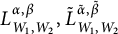be the source-to-solution maps corresponding to $g, \tilde {g}$ . Suppose $g= \tilde {g}$ in $W_1\cup W_2$ and

(3) $$ \begin{align} L^{\alpha, \beta}_{W_1, W_2} f= \tilde{L}^{\tilde{\alpha}, \tilde{\beta}}_{W_1, W_2} f,\qquad f\in C^2_c((0, \infty); L^2(W_1)). \end{align} $$

Then $\alpha = \tilde {\alpha }$ , $\beta = \tilde {\beta }$ , and $(M, g)$ and $(M, \tilde {g})$ are isometric Riemannian manifolds.

We remark that the case $\beta , \tilde {\beta }= 1/2$ has been excluded since we need to apply the unique continuation property of the fractional Laplace–Beltrami operator (Proposition 2.1) after (13).

1.1 Connection with earlier literature

Inverse spectral theory and the associated metric determination problem for hyperbolic equations have been extensively studied so far. The approach mainly relies on the boundary control method (see [Reference Belishev and Kurylev4]) and its variant. We refer readers to the textbook [Reference Kachalov, Kurylev and Lassas18] for a detailed study of this topic. We also refer readers to [Reference Helin, Lassas, Oksanen and Saksala15, Reference Krupchyk, Kurylev and Lassas20, Reference Lassas, Nursultanov, Oksanen and Ylinen25, Reference Lassas and Oksanen26, Reference Li and Zhang28] for metric determination results on manifolds with or without boundary.

There is also abundant literature available on inverse problems for fractional operators. The rigorous mathematical study of inverse problems for time-fractional but space-local equations at least dates back the late 2000s (see, for instance, [Reference Cheng, Nakagawa, Yamamoto and Yamazaki5, Reference Kian, Li, Liu and Yamamoto19]). The study of Calderón-type inverse problems for space-fractional equations was initiated in [Reference Ghosh, Salo and Uhlmann13]. We refer readers to [Reference Covi6, Reference Covi, Mönkkönen, Railo and Uhlmann7, Reference Ghosh, Rüland, Salo and Uhlmann12, Reference Lai and Zhou22] and the references inside for extended results for the fractional Calderón problem and its variants. In particular, we mention that the Calderón-type inverse problem for the (coupled or uncoupled) space–time fractional parabolic equations has been studied in [Reference Lai, Lin and Rüland21, Reference Li27]. We also mention that the determination result for exponents in the space–time fractional diffusion equation (in 1-dim case) has been obtained in [Reference Tatar, Tinaztepe and Ulusoy34].

In addition, there are a few recent works on the metric determination for fractional equations. One seminal work is [Reference Feizmohammadi, Ghosh, Krupchyk and Uhlmann9], where the authors reduced the fractional elliptic problem to the classical hyperbolic problem by taking advantage of the semigroup definition of the fractional operator and the transmutation formula. Concerning the model in this article, a more related work is [Reference Helin, Lassas, Ylinen and Zhang16], where the authors determined the metric up to an isometry from the knowledge of the source-to-solution map associated with the space–time fractional diffusion equation.

In this article, we seek a simultaneous determination of the exponents and the metric in the space–time fractional Schrödinger equation, and the proof of the main theorem involves a combination of different kinds of techniques. More precisely, our determination of the time-fractional power $\alpha $ relies on the asymptotic behavior of Mittag-Leffler functions and the unique continuation property of the space-fractional operator. Our determination of the space-fractional power $\beta $ and the metric g relies on Weyl’s law for the eigenvalues and the disjoint data metric determination result for the wave equation established in [Reference Lassas, Nursultanov, Oksanen and Ylinen25].

1.2 Organization

The rest of this article is organized in the following way. In Section 2, we will summarize the preliminary knowledge. In Section 3, we will study the well-posedness of (1) for sufficiently smooth sources. In Section 4, we will prove the main theorem. In Section 5, we will provide a probabilistic formulation of our inverse problem.

2 Preliminaries

Throughout this article, the space dimension $n\geq 2$ . We use $\langle \cdot , \cdot \rangle $ to denote the $L^2$ -inner product, and we use $\alpha , \beta \in (0, 1)$ to denote constant fractional powers.

2.1 Laplace–Beltrami operator and Sobolev spaces

Let $(M, g)$ be a smooth connected closed manifold. Let $0= \lambda _0< \lambda _1\leq \lambda _2<\cdots \to +\infty $ be the eigenvalues of the Laplace–Beltrami operator $-\Delta _g$ . Then there exists an orthonormal basis of $L^2(M)$ consisting of the eigenfunctions $\varphi _k$ corresponding to $\lambda _k$ . Recall that for $r\geq 0$ ,

$$ \begin{align*}H^r(M) = \{u \in L^2(M): \sum_{k=1}^\infty \lambda_k^{r} |\langle u, \varphi_k \rangle|^2 < +\infty\}.\end{align*} $$

The fractional operator $(-\Delta _g)^r$ is defined by

(4) $$ \begin{align} (-\Delta_g)^r u:=\sum_{k=1}^\infty \lambda_k^r \langle u, \varphi_k \rangle\varphi_k,\qquad u\in H^{2r}(M). \end{align} $$

We say that a nonempty open subset $W\subset M$ satisfies the spectral bound condition provided that there exists a constant $C_0> 0$ such that for any basis of normalized eigenfunctions $\{\varphi _k\}$ of the Laplace–Beltrami operator, the estimate

(5) $$ \begin{align} 1\leq C_0||\varphi_k||_{L^2(W)} \end{align} $$

holds for all $k\in \mathbb {N}$ . We remark that this condition holds true for an Anosov surface, regardless of the specific choice of W. We refer readers to [Reference Lassas, Nursultanov, Oksanen and Ylinen25] for more details of the Anosov property.

We will later use the following unique continuation property on closed manifolds.

Proposition 2.1 Let $r\in (0, \infty )\setminus \mathbb {N}$ . Let $W\subset M$ be nonempty and open. Suppose that $u\in C^{\infty }(M)$ satisfies

$$ \begin{align*}(-\Delta_g)^r u= u= 0\end{align*} $$

in W. Then $u= 0$ in M.

We remark that the unique continuation property of the fractional Laplacian in $\mathbb {R}^n$ was first proved in [Reference Ghosh, Salo and Uhlmann13] based on the Carleman estimates in [Reference Rüland33]. We also remark that Proposition 2.1 can be viewed as a special case of the more general entanglement principle (see Theorem 1.8 in [Reference Feizmohammadi, Krupchyk and Uhlmann10]).

2.2 Caputo derivatives and Mittag-Leffler functions

For $u(t)\in C^1([0, \infty ))$ , its Caputo derivative is given by

(6) $$ \begin{align} \partial_t^\alpha u(t)= \frac{1}{\Gamma(1-\alpha)}\int^t_0\frac{u'(\tau)}{(t-\tau)^\alpha}\,\mathrm{d}\tau. \end{align} $$

If $u(0)= 0$ , then we have the following Laplace transform formula

$$ \begin{align*}\mathcal{L}(\partial_t^\alpha u)(s)= s^\alpha \mathcal{L}u (s).\end{align*} $$

For $u(t)\in C^1([0, \infty ); L^2(M))$ , the integral in (6) should be interpreted in the sense of Bochner.

For $a, b> 0$ , we have the (two-parameter) Mittag-Leffler function

$$ \begin{align*}E_{a,b}(z):= \sum^\infty_{k=0}\frac{z^k}{\Gamma(ka+b)},\end{align*} $$ upper E Subscript a comma b Baseline left parenthesis z right parenthesis colon equals sigma summation Underscript k equals 0 Overscript infinity Endscripts StartFraction z Superscript k Baseline Over normal upper Gamma left parenthesis k a plus b right parenthesis EndFraction comma

which is an entire function generalizing the exponential function $e^z= E_{1,1}(z)$ . Here, $\Gamma $ is the standard Gamma function. For fixed a, we define

$$ \begin{align*}G_\xi(z):= E_{a, 1}(-\xi z^a)\end{align*} $$

for each $\xi \in \mathbb {C}$ , which is holomorphic on $\{z\in \mathbb {C}: \mathrm {Re}\,z> 0\}$ . Based on the relation $\Gamma (z+1)= z\Gamma (z)$ , it is easy to verify that

(7) $$ \begin{align} \frac{\mathrm{d}}{\mathrm{d}z}G_\xi(z)= -\xi z^{a-1}E_{a, a}(-\xi z^a). \end{align} $$

The following proposition corresponds to Theorems 1.4 and 1.6 in [Reference Podlubny32].

Proposition 2.2 Suppose $0< a< 2$ , $b> 0,$ and $\pi a/2< \mu < \min \{\pi , \pi a\}$ . Then we have

$$ \begin{align*}|E_{a,b}(z)|\leq \frac{C}{1+ |z|},\qquad \mu\leq |\arg(z)|\leq \pi\end{align*} $$

for some positive constant C. We also have

$$ \begin{align*}E_{a,1}(z)= -\frac{z^{-1}}{\Gamma(1-\alpha)}+ \mathrm{O}(|z|^{-2}),\qquad \mu\leq |\arg(z)|\leq \pi\end{align*} $$

as $|z|\to \infty $ .

In particular, since $0< \alpha < 1$ , we can choose $a= \alpha $ , $\pi \alpha /2 < \mu < \min \{\pi /2, \pi \alpha \}$ in the proposition above, which implies $E_{\alpha , \alpha }$ and $E_{\alpha , 1}$ are bounded on the imaginary axis, and $E_{\alpha , 1}$ has the above asymptotic expansion on the imaginary axis.

3 Well-posedness

Our goal here is to establish the well-posedness of (1). We are not going to pursue the optimal regularity since this is not our main concern.

Proposition 3.1 For $f\in C^2_c((0, \infty ); L^2(M))$ , there exists a unique solution of (1) satisfying

$$ \begin{align*}u\in C^1([0, \infty); H^{2\beta}(M))\cap L^\infty([0, \infty); H^{2\beta}(M)),\quad \partial_t u\in L^\infty([0, \infty); H^{2\beta}(M)).\end{align*} $$

Proof Recall that the fractional operator $(-\Delta _g)^r$ is defined by (4). Hence, it is natural to construct the solution in the series form of $\sum ^\infty _{k= 0}u_k(t)\varphi _k$ 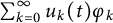. To determine the Fourier coefficients $u_k$ , we need to solve the fractional ODE

(8) $$ \begin{align} \left\{ \begin{aligned} (i\partial_t^\alpha + \lambda^\beta_k) u_k&= f_k,\\ u_k(0)&= 0,\\ \end{aligned} \right. \end{align} $$

where $f_k(t)= \langle f(t), \varphi _k\rangle \in C^2_c((0, \infty ))$ . Based on the convolution property of the Laplace transform, this fractional ODE has the solution

(9) $$ \begin{align} u_k = K_k* f_k \end{align} $$

(see (7) in [Reference Ashurov and Shakarova3]), where $K_k(t)$ satisfies the Laplace transform

(10) $$ \begin{align} \mathcal{L}K_k(s)= \frac{1}{is^\alpha+ \lambda^\beta_k}. \end{align} $$ script upper L upper K Subscript k Baseline left parenthesis s right parenthesis equals StartFraction 1 Over i s Superscript alpha Baseline plus lamda Subscript k Superscript beta Baseline EndFraction period

Based on the formula (4.9.1) in [Reference Gorenflo, Kilbas, Mainardi and Rogosin14], we know that

(11) $$ \begin{align} K_k(t)= -it^{\alpha-1}E_{\alpha, \alpha}(i\lambda^\beta_k t^\alpha). \end{align} $$

The $j^{th}$ derivatives of $u_k$ (with respect to time) satisfies

$$ \begin{align*}u^{(j)}_k = K_k* f^{(j)}_k,\qquad j= 0, 1.\end{align*} $$

Then we have

$$ \begin{align*}\lambda^\beta_ku^{(j)}_k(t)&= \int^t_0 -i\lambda^\beta_k(t-\tau)^{\alpha-1} E_{\alpha, \alpha}(i\lambda^\beta_k (t-\tau)^\alpha)f^{(j)}_k(\tau)\,d\tau\\ &= \int^t_0 [\frac{\mathrm{d}}{\mathrm{d}\tau} E_{\alpha, 1}(i\lambda^\beta_k (t-\tau)^\alpha)]f^{(j)}_k(\tau)\,d\tau\end{align*} $$

StartLayout 1st Row 1st Column lamda Subscript k Superscript beta Baseline u Subscript k Superscript left parenthesis j right parenthesis Baseline left parenthesis t right parenthesis 2nd Column equals integral Subscript 0 Superscript t Baseline minus i lamda Subscript k Superscript beta Baseline left parenthesis t minus tau right parenthesis Superscript alpha minus 1 Baseline upper E Subscript alpha comma alpha Baseline left parenthesis i lamda Subscript k Superscript beta Baseline left parenthesis t minus tau right parenthesis Superscript alpha Baseline right parenthesis f Subscript k Superscript left parenthesis j right parenthesis Baseline left parenthesis tau right parenthesis d tau 2nd Row 1st Column Blank 2nd Column equals integral Subscript 0 Superscript t Baseline left bracket StartFraction normal d Over normal d tau EndFraction upper E Subscript alpha comma 1 Baseline left parenthesis i lamda Subscript k Superscript beta Baseline left parenthesis t minus tau right parenthesis Superscript alpha Baseline right parenthesis right bracket f Subscript k Superscript left parenthesis j right parenthesis Baseline left parenthesis tau right parenthesis d tau EndLayout

by (7). Using $E_{a, 1}(0)= 1$ , $f^{(j)}_k(0)= 0$ , we integrate by parts to obtain

(12) $$ \begin{align} \lambda^\beta_ku^{(j)}_k(t)= f^{(j)}_k(t)- \int^t_0E_{\alpha, 1}(i\lambda^\beta_k (t-\tau)^\alpha)f^{(j+1)}_k(\tau)d\tau. \end{align} $$

Then we have

$$ \begin{align*}\lambda^\beta_k|u^{(j)}_k(t)| &\leq |f^{(j)}_k(t)|+ \int^t_0|E_{\alpha, 1}(i\lambda^\beta_k (t-\tau)^\alpha)f^{(j+1)}_k(\tau)|d\tau\\&\leq \int^t_0(1+|E_{\alpha, 1}(i\lambda^\beta_k (t-\tau)^\alpha)|)|f^{(j+1)}_k(\tau)|d\tau.\end{align*} $$

StartLayout 1st Row 1st Column lamda Subscript k Superscript beta Baseline StartAbsoluteValue u Subscript k Superscript left parenthesis j right parenthesis Baseline left parenthesis t right parenthesis EndAbsoluteValue 2nd Column less than or equals StartAbsoluteValue f Subscript k Superscript left parenthesis j right parenthesis Baseline left parenthesis t right parenthesis EndAbsoluteValue plus integral Subscript 0 Superscript t Baseline StartAbsoluteValue upper E Subscript alpha comma 1 Baseline left parenthesis i lamda Subscript k Superscript beta Baseline left parenthesis t minus tau right parenthesis Superscript alpha Baseline right parenthesis f Subscript k Superscript left parenthesis j plus 1 right parenthesis Baseline left parenthesis tau right parenthesis EndAbsoluteValue d tau 2nd Row 1st Column Blank 2nd Column less than or equals integral Subscript 0 Superscript t Baseline left parenthesis 1 plus StartAbsoluteValue upper E Subscript alpha comma 1 Baseline left parenthesis i lamda Subscript k Superscript beta Baseline left parenthesis t minus tau right parenthesis Superscript alpha Baseline right parenthesis EndAbsoluteValue right parenthesis StartAbsoluteValue f Subscript k Superscript left parenthesis j plus 1 right parenthesis Baseline left parenthesis tau right parenthesis EndAbsoluteValue d tau period EndLayout

Suppose $\mathrm {supp}\,f\subset (0, T_0)\times M$ for some $T_0> 0$ . By the boundedness of $E_{\alpha , 1}$ on the imaginary axis and Cauchy–Schwarz inequality, we have

$$ \begin{align*}\lambda^{2\beta}_k|u^{(j)}_k(t)|^2 &\leq \int^{\min\{t, T_0\}}_0 (1+ |E_{\alpha, 1}(i\lambda^\beta_k (t-\tau)^\alpha)|)^2 d\tau \int^{\min\{t, T_0\}}_0|f^{(j+1)}_k(\tau)|^2 d\tau\\&\leq C_\alpha T_0 \int^{T_0}_0|f^{(j+1)}_k(\tau)|^2 d\tau.\end{align*} $$

StartLayout 1st Row 1st Column lamda Subscript k Superscript 2 beta Baseline StartAbsoluteValue u Subscript k Superscript left parenthesis j right parenthesis Baseline left parenthesis t right parenthesis EndAbsoluteValue squared 2nd Column less than or equals integral Subscript 0 Superscript min left brace t comma upper T 0 right brace Baseline left parenthesis 1 plus StartAbsoluteValue upper E Subscript alpha comma 1 Baseline left parenthesis i lamda Subscript k Superscript beta Baseline left parenthesis t minus tau right parenthesis Superscript alpha Baseline right parenthesis EndAbsoluteValue right parenthesis squared d tau integral Subscript 0 Superscript min left brace t comma upper T 0 right brace Baseline StartAbsoluteValue f Subscript k Superscript left parenthesis j plus 1 right parenthesis Baseline left parenthesis tau right parenthesis EndAbsoluteValue squared d tau 2nd Row 1st Column Blank 2nd Column less than or equals upper C Subscript alpha Baseline upper T 0 integral Subscript 0 Superscript upper T 0 Baseline StartAbsoluteValue f Subscript k Superscript left parenthesis j plus 1 right parenthesis Baseline left parenthesis tau right parenthesis EndAbsoluteValue squared d tau period EndLayout

By the dominated convergence theorem,

$$ \begin{align*}\sum^\infty_{k= N}\lambda_k^{2\beta} |u^{(j)}_k(t)|^2\leq C_\alpha T_0\int^{T_0}_0\sum^\infty_{k= N}|f^{(j+1)}_k(\tau)|^2\,d\tau\to 0\end{align*} $$

as $N\to \infty $ . This convergence (uniform in $t\in [0, \infty )$ ) implies that $\sum ^\infty _{k= 0}u^{(j)}_k(t)\varphi _k$ 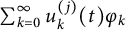( $j= 0, 1$ ) converges uniformly in $H^{2\beta }(M)$ . Hence, we can differentiate

$$ \begin{align*}u(t):=\sum^\infty_{k= 0}u_k(t)\varphi_k\end{align*} $$ StartLayout 1st Row u left parenthesis t right parenthesis colon equals sigma summation Underscript k equals 0 Overscript infinity Endscripts u Subscript k Baseline left parenthesis t right parenthesis phi Subscript k EndLayout

with respect to t term-by-term. Now, by the definition of Caputo derivatives (6) and Proposition 23 in [Reference Helin, Lassas, Ylinen and Zhang16], we have

$$ \begin{align*}\partial^\alpha_t u(t)=\sum^\infty_{k= 0}\partial^\alpha_t u_k(t)\varphi_k.\end{align*} $$ StartLayout 1st Row partial differential Subscript t Superscript alpha Baseline u left parenthesis t right parenthesis equals sigma summation Underscript k equals 0 Overscript infinity Endscripts partial differential Subscript t Superscript alpha Baseline u Subscript k Baseline left parenthesis t right parenthesis phi Subscript k Baseline period EndLayout

Hence, (8) ensures that $\sum ^\infty _{k= 0}u_k(t)\varphi _k$ 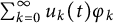is the solution of (1).

For uniqueness, it suffices to show that a solution u of (1) has to be zero in the homogeneous case $f= 0$ . In fact, we have $u_k(t)= \langle u(t), \varphi _k\rangle \in C^1([0, \infty ))$ and $u^{\prime }_k(t)= \langle u'(t), \varphi _k\rangle $ for $u\in C^1([0, \infty ); L^2(M))$ . Again by Proposition 23 in [Reference Helin, Lassas, Ylinen and Zhang16], we further have

$$ \begin{align*}\langle\partial^\alpha_t u(t), \varphi_k\rangle =\frac{1}{\Gamma(1-\alpha)}\int^t_0\frac{u^{\prime}_k(\tau)}{(t-\tau)^\alpha}\,\mathrm{d}\tau = \partial^\alpha_t u_k(t).\end{align*} $$

Hence, if $f= 0$ , then $u_k$ satisfies (8) in the homogeneous case $f_k= 0$ , which has the unique solution $u_k= 0$ (see Lemma 2 in [Reference Ashurov and Shakarova3]).

4 Inverse problem

Our goal here is to prove Theorem 1.1.

Let $\lambda _{j_k}$ be the distinct eigenvalues and $P_k$ be the projections on the corresponding eigenspaces spanned by the eigenfunctions $\varphi _{j_k, p}$ ( $1\leq p\leq m_k$ ). Here, $m_k$ are the corresponding multiplicities. Then we have

$$ \begin{align*}P_k u= \sum^{m_k}_{p=1}\langle u, \varphi_{j_k, p} \rangle \varphi_{j_k, p},\qquad u\in L^2(M).\end{align*} $$ upper P Subscript k Baseline u equals sigma summation Underscript p equals 1 Overscript m Subscript k Baseline Endscripts left angle bracket u comma phi Subscript j Sub Subscript k Subscript comma p Baseline right angle bracket phi Subscript j Sub Subscript k Subscript comma p Baseline comma u element of upper L squared left parenthesis upper M right parenthesis period

We define

$$ \begin{align*}P_{W_1, W_2, k}:= (P_k\circ e)|_{W_2},\end{align*} $$

where e is the zero extension map from $L^2(W_1)$ to $L^2(M)$ . Note that

$$ \begin{align*}P_{W_1, W_2, k}\in B(L^2(W_1)\to L^2(W_2)),\end{align*} $$

which denotes the space of bounded linear operators from $L^2(W_1)$ to $L^2(W_2)$ .

Due to the unique continuation property of elliptic operators, $\{\varphi _{j_k, p}|_{W_l}\}^{m_k}_{p=1}$ 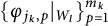are linearly independent functions for $l= 1, 2$ . If

$$ \begin{align*}\sum^{m_k}_{p=1} c_pP_{W_1, W_2, k}(\varphi_{j_k, p}|_{W_1})= 0,\end{align*} $$ sigma summation Underscript p equals 1 Overscript m Subscript k Baseline Endscripts c Subscript p Baseline upper P Subscript upper W 1 comma upper W 2 comma k Baseline left parenthesis phi Subscript j Sub Subscript k Subscript comma p Baseline vertical bar Subscript upper W 1 Baseline right parenthesis equals 0 comma

then it implies that

$$ \begin{align*}\langle \sum^{m_k}_{p=1} c_pe(\varphi_{j_k, p}|_{W_1}), \varphi_{j_k, l}\rangle= 0, \qquad 1\leq l\leq m_k\end{align*} $$

based on the linear independence of $\{\varphi _{j_k, p}|_{W_2}\}^{m_k}_{p=1}$ 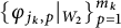. Combining these $m_k$ identities, it further implies

$$ \begin{align*}\sum^{m_k}_{p=1} c_p\varphi_{j_k, p}|_{W_1}= 0,\end{align*} $$ sigma summation Underscript p equals 1 Overscript m Subscript k Baseline Endscripts c Subscript p Baseline phi Subscript j Sub Subscript k Subscript comma p Baseline vertical bar Subscript upper W 1 Baseline equals 0 comma

and thus $c_p= 0$ for $1\leq p\leq m_k$ based on the linear independence of $\{\varphi _{j_k, p}|_{W_1}\}^{m_k}_{p=1}$ 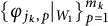. Hence, $P_{W_1, W_2, k}$ has rank $m_k$ , and thus it is not a zero map for each k.

We remark that based on the formula (4.9.1) in [Reference Gorenflo, Kilbas, Mainardi and Rogosin14], the Laplace transform formula (10) is valid for s with $\mathrm {Re}\,s> \lambda _k^{\frac {\beta }{\alpha }}$ . By the boundedness of $E_{\alpha , \alpha }$ on the imaginary axis, the Laplace transform on the LHS of (10) is well-defined for s with $\mathrm {Re}\,s> 0$ , so the analytic continuation implies that (10) is valid for s with $\mathrm {Re}\,s> 0$ .

To prove Theorem 1.1, we will first determine the time-fractional power $\alpha $ and then determine the space-fractional power $\beta $ and the metric g up to an isometry.

4.1 Determination of the time-fractional power

Roughly speaking, we will choose specific sources and study the asymptotic behavior of the corresponding solutions for large time t. The unique continuation property of the fractional Laplace–Beltrami operator will ensure that the principal part in the asymptotic expansion is non-vanishing. Then the knowledge of the source-to-solution map will enable us to determine the time-fractional power $\alpha $ .

More precisely, we pick a nonzero $\xi \in C^\infty _c(W_1)$ 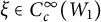s.t. $\langle e(\xi ), 1\rangle = 0$ 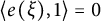. For each $t> 0$ , we define

$$\begin{align*}g_t(\tau):=\begin{cases} \tau, & 0\leq \tau\leq t/3;\\ 2t/3-\tau, & t/3\leq \tau\leq 2t/3;\\ 0, & 2t/3\leq \tau\leq t. \end{cases} \end{align*}$$

g Subscript t Baseline left parenthesis tau right parenthesis colon equals StartLayout Enlarged left brace 1st Row 1st Column tau comma 2nd Column 0 less than or equals tau less than or equals t divided by 3 semicolon 2nd Row 1st Column 2 t divided by 3 minus tau comma 2nd Column t divided by 3 less than or equals tau less than or equals 2 t divided by 3 semicolon 3rd Row 1st Column 0 comma 2nd Column 2 t divided by 3 less than or equals tau less than or equals t period EndLayout

Note that $g_t$ is absolutely continuous and weakly differentiable, and we can choose (scalar-valued) functions $^l f(\tau )\in C^2_c((0, t))$ s.t. $^l f\to g_t$ in $H^1$ as $l\to \infty $ . Let $^l u$ be the solution corresponding to the source $(^l f)e(\xi )$ . We use $(^l u)_k$ to denote the Fourier coefficients of $^l u$ . Then, by (12), we have

$$ \begin{align*}\lambda^\beta_k (^l u)_k(t)= -(\int^t_0 E_{\alpha, 1}(i\lambda^\beta_k (t-\tau)^\alpha) (^l f)'(\tau)d\tau) \langle e(\xi), \varphi_k\rangle.\end{align*} $$

The knowledge of the source-to-solution map $L^{\alpha , \beta }_{W_1, W_2}$ gives the knowledge of $(^l u)(t)|_{W_2}$ for each l. Let $l\to \infty $ . Then we have the knowledge of $w(t)|_{W_2}$ . Here,

$$ \begin{align*}w&= -\sum^\infty_{k=1}\frac{1}{\lambda^\beta_k}(\int^t_0 E_{\alpha, 1}(i\lambda^\beta_k (t-\tau)^\alpha) (g_t)'(\tau)d\tau) \langle e(\xi), \varphi_k\rangle\varphi_k\\&= -\sum^\infty_{k=1}\frac{1}{\lambda^\beta_k}[\int^{t/3}_0 E_{\alpha, 1}(i\lambda^\beta_k (t-\tau)^\alpha) d\tau- \int^{2t/3}_{t/3} E_{\alpha, 1}(i\lambda^\beta_k (t-\tau)^\alpha) d\tau] \langle e(\xi), \varphi_k\rangle\varphi_k.\end{align*} $$

StartLayout 1st Row 1st Column w 2nd Column equals minus sigma summation Underscript k equals 1 Overscript infinity Endscripts StartFraction 1 Over lamda Subscript k Superscript beta Baseline EndFraction left parenthesis integral Subscript 0 Superscript t Baseline upper E Subscript alpha comma 1 Baseline left parenthesis i lamda Subscript k Superscript beta Baseline left parenthesis t minus tau right parenthesis Superscript alpha Baseline right parenthesis left parenthesis g Subscript t Baseline right parenthesis prime left parenthesis tau right parenthesis d tau right parenthesis left angle bracket e left parenthesis xi right parenthesis comma phi Subscript k Baseline right angle bracket phi Subscript k Baseline 2nd Row 1st Column Blank 2nd Column equals minus sigma summation Underscript k equals 1 Overscript infinity Endscripts StartFraction 1 Over lamda Subscript k Superscript beta Baseline EndFraction left bracket integral Subscript 0 Superscript t divided by 3 Baseline upper E Subscript alpha comma 1 Baseline left parenthesis i lamda Subscript k Superscript beta Baseline left parenthesis t minus tau right parenthesis Superscript alpha Baseline right parenthesis d tau minus integral Subscript t divided by 3 Superscript 2 t divided by 3 Baseline upper E Subscript alpha comma 1 Baseline left parenthesis i lamda Subscript k Superscript beta Baseline left parenthesis t minus tau right parenthesis Superscript alpha Baseline right parenthesis d tau right bracket left angle bracket e left parenthesis xi right parenthesis comma phi Subscript k Baseline right angle bracket phi Subscript k Baseline period EndLayout

Note that $|i\lambda ^\beta _k (t-\tau )^\alpha |\geq \lambda ^\beta _1(\frac {t}{3})^\alpha $ for $\tau \in [0, 2t/3]$ . Then we use the asymptotic expansion of $E_{\alpha , 1}$ in Proposition 2.2 for large t to obtain

$$ \begin{align*}&\int^{t/3}_0 E_{\alpha, 1}(i\lambda^\beta_k (t-\tau)^\alpha) d\tau- \int^{2t/3}_{t/3} E_{\alpha, 1}(i\lambda^\beta_k (t-\tau)^\alpha) d\tau\\&\quad =c_\alpha[\frac{(t-\tau)^{1-\alpha}}{\lambda^\beta_k}|^{\tau=t/3}_{\tau= 0}- \frac{(t-\tau)^{1-\alpha}}{\lambda^\beta_k}|^{\tau=2t/3}_{\tau= t/3}]+ \frac{1}{\lambda^{2\beta}_k}\mathrm{O}(t^{1-2\alpha}).\end{align*} $$

StartLayout 1st Row 1st Column Blank 2nd Column integral Subscript 0 Superscript t divided by 3 Baseline upper E Subscript alpha comma 1 Baseline left parenthesis i lamda Subscript k Superscript beta Baseline left parenthesis t minus tau right parenthesis Superscript alpha Baseline right parenthesis d tau minus integral Subscript t divided by 3 Superscript 2 t divided by 3 Baseline upper E Subscript alpha comma 1 Baseline left parenthesis i lamda Subscript k Superscript beta Baseline left parenthesis t minus tau right parenthesis Superscript alpha Baseline right parenthesis d tau 2nd Row 1st Column Blank 2nd Column equals c Subscript alpha Baseline left bracket StartFraction left parenthesis t minus tau right parenthesis Superscript 1 minus alpha Baseline Over lamda Subscript k Superscript beta Baseline EndFraction vertical bar Subscript tau equals 0 Superscript tau equals t divided by 3 Baseline minus StartFraction left parenthesis t minus tau right parenthesis Superscript 1 minus alpha Baseline Over lamda Subscript k Superscript beta Baseline EndFraction vertical bar Subscript tau equals t divided by 3 Superscript tau equals 2 t divided by 3 Baseline right bracket plus StartFraction 1 Over lamda Subscript k Superscript 2 beta Baseline EndFraction normal upper O left parenthesis t Superscript 1 minus 2 alpha Baseline right parenthesis period EndLayout

Hence, we can write

$$ \begin{align*}w= C_{\alpha}t^{1-\alpha}\omega+ \mathrm{O}(t^{1-2\alpha}),\quad \omega= \sum^\infty_{k=1}\frac{1}{\lambda^{2\beta}_k}\langle e(\xi), \varphi_k\rangle\varphi_k.\end{align*} $$

Here, $c_{\alpha }, C_{\alpha }$ are nonzero constants only depending on $\alpha $ , and the asymptotic expansion is in $H^{4\beta }(M)$ -norm. Note that we have $(-\Delta _g)^{2\beta }\omega = e(\xi )$ and $\omega \in C^\infty (M)$ . Since $W_1$ and $W_2$ are disjoint based on the assumption in the statement of Theorem 1.1, we claim that $\omega |_{W_2}$ is nonzero. Otherwise,

(13) $$ \begin{align} (-\Delta_g)^{2\beta}\omega= \omega =0 \end{align} $$

in $W_2$ implies $\omega \equiv 0$ by the unique continuation property (Proposition 2.1), which contradicts with our choice of $\xi $ .

We can do the same analysis for $\tilde {L}^{\tilde {\alpha }, \tilde {\beta }}_{W_1, W_2}$ . Then $L^{\alpha , \beta }_{W_1, W_2}= \tilde {L}^{\tilde {\alpha }, \tilde {\beta }}_{W_1, W_2}$ 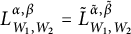implies

$$ \begin{align*}C_{\alpha}t^{1-\alpha}\omega|_{W_2}+ \mathrm{O}(t^{1-2\alpha})= \tilde{C}_{\tilde{\alpha}}t^{1-\tilde{\alpha}}\tilde{\omega}|_{W_2}+ \mathrm{O}(t^{1-2\tilde{\alpha}})\end{align*} $$

for large t. We conclude that $\alpha = \tilde {\alpha }$ . Otherwise, we may assume $\alpha < \tilde {\alpha }$ . Then we multiply both sides of the identity above by $t^{\alpha -1}$ and let $t\to \infty $ to reach the contradiction.

4.2 Determination of the space-fractional power and the metric

Now we can fix $\alpha $ since it has been determined. Next, we will retrieve the spectral information via the Laplace transform with respect to time. Weyl’s law will enable us to determine the space-fractional power $\beta $ , and the determination result for the wave equation will enable us to determine the metric g up to an isometry.

Proposition 4.1 The knowledge of $L^{\alpha , \beta }_{W_1, W_2}f$ for all $f\in C^2_c((0, \infty ); L^2(W_1))$ determines the operator-valued function

(14) $$ \begin{align} H^{\beta}_{W_1, W_2}(s):=\sum^\infty_{k=1}\frac{1}{\lambda^\beta_{j_k} + i s^\alpha }P_{W_1, W_2, k},\qquad \mathrm{Re}\,s> 0. \end{align} $$

Proof We fix a nonzero nonnegative $a(t)\in C^2_c((0, \infty ))$ such that $\mathcal {L}a> 0$ on $(0, \infty )$ . We consider a source f of the form

$$ \begin{align*}f= a(t)e(\xi),\qquad \xi\in L^2(W_1)\quad s.t.\quad \langle e(\xi), 1\rangle= 0.\end{align*} $$

(Then the Fourier coefficient $f_0 =0$ , and the summation will start at $k=1$ .)

Recall that we use $u_f$ to denote the solution of (1) associated with f. Then for each s with $\mathrm {Re}\,s> 0$ , the function $e^{-st}u_f(t)$ is $L^2$ -valued integrable on $(0, \infty )$ . By Proposition 23 in [Reference Helin, Lassas, Ylinen and Zhang16], we can take the Laplace transform componentwise. For $f= a(t)e(\xi )$ 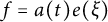, we use the convolution property of the Laplace transform to obtain

$$ \begin{align*}\mathcal{L}u_f(s)&= \sum^\infty_{k=1} \mathcal{L}(K_k* f_k)(s)\varphi_k= \sum^\infty_{k=1}\frac{1}{\lambda^\beta_k+ i s^\alpha}\mathcal{L}f_k(s)\varphi_k\\& = \sum^\infty_{k=1}\frac{1}{\lambda^\beta_k+ i s^\alpha}\langle\mathcal{L}f(s), \varphi_k\rangle\varphi_k= \mathcal{L}a(s)\sum^\infty_{k=1}\frac{1}{\lambda^\beta_{j_k}+ i s^\alpha}P_k\circ e(\xi)\end{align*} $$

StartLayout 1st Row 1st Column script upper L u Subscript f Baseline left parenthesis s right parenthesis 2nd Column equals sigma summation Underscript k equals 1 Overscript infinity Endscripts script upper L left parenthesis upper K Subscript k Baseline asterisk f Subscript k Baseline right parenthesis left parenthesis s right parenthesis phi Subscript k Baseline equals sigma summation Underscript k equals 1 Overscript infinity Endscripts StartFraction 1 Over lamda Subscript k Superscript beta Baseline plus i s Superscript alpha Baseline EndFraction script upper L f Subscript k Baseline left parenthesis s right parenthesis phi Subscript k Baseline 2nd Row 1st Column Blank 2nd Column equals sigma summation Underscript k equals 1 Overscript infinity Endscripts StartFraction 1 Over lamda Subscript k Superscript beta Baseline plus i s Superscript alpha Baseline EndFraction left angle bracket script upper L f left parenthesis s right parenthesis comma phi Subscript k Baseline right angle bracket phi Subscript k Baseline equals script upper L a left parenthesis s right parenthesis sigma summation Underscript k equals 1 Overscript infinity Endscripts StartFraction 1 Over lamda Subscript j Sub Subscript k Subscript Superscript beta Baseline plus i s Superscript alpha Baseline EndFraction upper P Subscript k Baseline ring e left parenthesis xi right parenthesis EndLayout

based on the formula for the solution of (1) in the proof of Proposition 3.1. Hence, we can conclude that $L^{\alpha , \beta }_{W_1, W_2}f$ determines the restriction of $\frac {1}{\mathcal {L}a(s)}\mathcal {L}u_f(s)$ 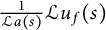in $W_2$ , which equals to $H^{\beta }_{W_1, W_2}(s)\xi $ .

In particular, the knowledge of $H^{\beta }_{W_1, W_2}(s)$ in (14) for $s>0$ determines the meromorphic operator-valued function

(15) $$ \begin{align} H^{\beta}_{W_1, W_2}(z):= \sum^\infty_{k=1}\frac{1}{\lambda^\beta_{j_k} + i z }P_{W_1, W_2, k} \end{align} $$ upper H Subscript upper W 1 comma upper W 2 Superscript beta Baseline left parenthesis z right parenthesis colon equals sigma summation Underscript k equals 1 Overscript infinity Endscripts StartFraction 1 Over lamda Subscript j Sub Subscript k Subscript Superscript beta Baseline plus i z EndFraction upper P Subscript upper W 1 comma upper W 2 comma k

with poles $\{i\lambda ^\beta _{j_k}\}$ . The convergence of the series in $B(L^2(W_1)\to L^2(W_2))$ -norm at non-pole z is ensured by the fact that $\lambda _{j_k}\to \infty $ as $k\to \infty $ and the fact that the operators $P_k$ project onto mutually orthogonal subspaces. Note that

$$ \begin{align*}\lim_{z\to z_0}(\lambda^\beta_{j_k} + i z)H^{\beta}_{W_1, W_2}(z)= P_{W_1, W_2, k}\end{align*} $$

if $z_0= i\lambda ^\beta _{j_k}$ , and the limit is zero if $z_0$ is not a pole.

Proposition 4.2 Let $H^{\beta }_{W_1, W_2}(z)$ and $\tilde {H}^{\tilde \beta }_{W_1, W_2}(z)$ be the meromorphic functions associated with g and $\tilde {g}$ , respectively. Suppose $g= \tilde {g}$ in $W_1\cup W_2$ and $H^{\beta }_{W_1, W_2}(z)= \tilde {H}^{\tilde \beta }_{W_1, W_2}(z)$ . Then we have $\beta = \tilde {\beta }$ and

$$ \begin{align*}\{(\lambda_{j_k}, P_{W_1, W_2, k}): k\in \mathbb{N}\}= \{(\tilde{\lambda}_{\tilde{j}_k}, \tilde{P}_{W_1, W_2, k}): k\in \mathbb{N}\}. \end{align*} $$

Proof Based on the assumption, for each $k \in \mathbb {N}$ , we have

(16) $$ \begin{align} P_{W_1, W_2, k}= \lim_{z\to i\lambda^\beta_{j_k}}(\lambda^\beta_{j_k} + i z)H^{\beta}_{W_1, W_2}(z) =\lim_{z\to i\lambda^\beta_{j_k}}(\lambda^\beta_{j_k} + i z)\tilde{H}^{\tilde\beta}_{W_1, W_2}(z). \end{align} $$

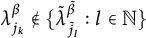
Note that the RHS of (16) equals to $\tilde {P}_{W_1, W_2, l}$ , provided $\lambda ^{\beta }_{j_k}= \tilde {\lambda }^{\tilde \beta }_{\tilde {j}_l}$ for some $l\in \mathbb {N}$ . Also note that if $\lambda ^{\beta }_{j_k}\notin \{\tilde {\lambda }^{\tilde \beta }_{\tilde {j}_l}: l\in \mathbb {N}\}$ , then $i\lambda ^\beta _{j_k}$ cannot be a pole of the $\tilde {H}^{\tilde \beta }_{W_1, W_2}(z)$ based on the previous observation, which implies that the RHS of (16) is zero contradicting with that $P_{W_1, W_2, k}$ is nonzero.

Hence, (16) implies

$$ \begin{align*}(\lambda^{\beta}_{j_k}, P_{W_1, W_2, k})\in \{(\tilde{\lambda}^{\tilde\beta}_{\tilde{j}_k}, \tilde{P}_{W_1, W_2, k}): k\in \mathbb{N}\}\end{align*} $$

for each k, and thus

$$ \begin{align*}\{(\lambda^{\beta}_{j_k}, P_{W_1, W_2, k}): k\in \mathbb{N}\}\subset \{(\tilde{\lambda}^{\tilde\beta}_{\tilde{j}_k}, \tilde{P}_{W_1, W_2, k}): k\in \mathbb{N}\}. \end{align*} $$

We can symmetrically show the reverse inclusion. Hence, we have

$$ \begin{align*}\{(\lambda^{\beta}_{j_k}, P_{W_1, W_2, k}): k\in \mathbb{N}\}= \{(\tilde{\lambda}^{\tilde\beta}_{\tilde{j}_k}, \tilde{P}_{W_1, W_2, k}): k\in \mathbb{N}\}. \end{align*} $$

Now $\lambda ^{\beta }_{j_k}= \tilde {\lambda }^{\tilde \beta }_{\tilde {j}_k}$ and $P_{W_1, W_2, k}= \tilde {P}_{W_1, W_2, k}$ imply that $m_k= \tilde {m}_k$ and $\lambda ^{\beta }_k= \tilde {\lambda }^{\tilde \beta }_k$ . Let $N(\lambda )$ , $\tilde {N}(\lambda )$ denote the number of eigenvalues of the Laplace–Beltrami operator corresponding to g, $\tilde {g}$ (counting their multiplicities) less than or equal to $\lambda $ . 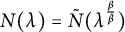Then $N(\lambda )= \tilde {N}(\lambda ^{\frac {\beta }{\tilde {\beta }}})$ . By Weyl’s law,

$$ \begin{align*}\lim_{\lambda\to \infty}\frac{N(\lambda)}{\lambda^{\frac{\mathrm{dim} M}{2}}}= C,\qquad \lim_{\lambda\to \infty}\frac{\tilde{N}(\lambda)}{\lambda^{\frac{\mathrm{dim} M}{2}}}= \tilde{C}.\end{align*} $$

Hence, the only possibility is $\beta = \tilde {\beta }$ . Then we have

$$ \begin{align*}\{(\lambda_{j_k}, P_{W_1, W_2, k}): k\in \mathbb{N}\}= \{(\tilde{\lambda}_{\tilde{j}_k}, \tilde{P}_{W_1, W_2, k}): k\in \mathbb{N}\}.\\[-34pt] \end{align*} $$

The proof of Theorem 1.1 will be complete based on the following known result since the source-to-solution map associated with the wave equation below is completely characterized by the spectral data set in Proposition 4.2.

Proposition 4.3 [Reference Lassas, Nursultanov, Oksanen and Ylinen25, Theorem 1.1]

Let $W_1, W_2\subset M$ be nonempty open subsets. Suppose $W_1$ satisfies the spectral bound condition (5) and $W_2$ has smooth boundary. The metric g can be determined up to an isometry from the knowledge of $g|_{W_1\cup W_2}$ and the source-to-solution map

$$ \begin{align*}L^{\mathrm{wave}}_{W_1, W_2}: f\to u_f|_{W_2\times (0, \infty)},\qquad f\in C^\infty_c((0, \infty)\times W_1)\end{align*} $$

associated with the wave equation

(17) $$ \begin{align} \left\{ \begin{aligned} (\partial^2_{t} -\Delta_g) u&= f,\quad \,\,\, (x, t)\in M\times (0, \infty),\\ u(0)= \partial_t u(0)&= 0,\quad \,\,\,x\in M.\\ \end{aligned} \right. \end{align} $$

Here, $L^{\mathrm {wave}}_{W_1, W_2}$ has the representation formula

$$ \begin{align*}L^{\mathrm{wave}}_{W_1, W_2}f(x, t)= \sum^\infty_{k=0}\int^t_0 K^{\mathrm{wave}}_{j_k}(t-\tau)P_{W_1, W_2, k}f(x, \tau)\,d\tau,\end{align*} $$

where $j_0= 0$ with

$$ \begin{align*}K^{\mathrm{wave}}_0(t)= t, \qquad K^{\mathrm{wave}}_k(t)= \frac{\sin(\sqrt{\lambda_k}t)}{\sqrt{\lambda_k}}\quad (k\geq 1).\end{align*} $$

5 Probabilistic formulation

Inverse problems for stochastic PDEs involving additive or multiplicative white noise have caught much attention recently (see, for instance, [Reference Feng, Li and Wang11, Reference Li, Chen and Li29]). Here, we will consider a stochastic version of the deterministic problem studied in previous sections.

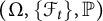
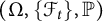
Throughout this section, we fix a filtered probability space $(\Omega , \{\mathcal {F}_t\}, \mathbb {P})$ . We use $\mathbb {E}$ to denote the expectation of a random variable, and we use $\dot {B}$ to denote the formal derivative of the standard real-valued Brownian motion $B_t$ defined on $(\Omega , \{\mathcal {F}_t\}, \mathbb {P})$ . For $\frac {1}{2}< \alpha < 1$ , we consider the fractional stochastic problem

(18) $$ \begin{align} \left\{ \begin{aligned} i\partial^\alpha_{t}u +(-\Delta_g)^\beta u &= f+ \sigma \dot {B},\quad \,\,\, \mathrm{in}\,\, M\times (0, \infty),\\ u(0)&= 0,\quad \,\,\,\mathrm{in}\,\, M,\\ \end{aligned} \right. \end{align} $$

where the mean of the source f and the deviation $\sigma $ are deterministic functions.

Definition 5.1. For $f, \sigma \in C^2_c((0, \infty ); L^2(M))$ , we say that u is the solution of (18) provided that

(19) $$ \begin{align} \sup_t\mathbb{E}[\,||u(t)||^2_{L^2(M)}\,]< \infty, \end{align} $$

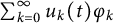
and u has the form $\sum ^\infty _{k= 0}u_k(t)\varphi _k$ , where the Fourier coefficients $u_k$ solve the fractional stochastic ODE

(20) $$ \begin{align} \left\{ \begin{aligned} (i\partial_t^\alpha + \lambda^\beta_k) u_k&= f_k+ \sigma_k \dot {B},\\ u_k(0)&= 0. \end{aligned} \right. \end{align} $$

Here, $f_k(t)= \langle f(t), \varphi _k\rangle \in C^2_c((0, \infty ))$ and $\sigma _k(t)= \langle \sigma (t), \varphi _k\rangle \in C^2_c((0, \infty ))$ .

We remark that (20) should be interpreted as the integral equation

(21) $$ \begin{align} u_k(t)= \frac{1}{\Gamma(\alpha)}\int^t_0 (t-\tau)^{\alpha-1}(i\lambda^\beta_k u_k(\tau)- if_k(\tau))\,\mathrm{d}\tau+ \frac{1}{\Gamma(\alpha)}\int^t_0 (t-\tau)^{\alpha-1}(- i\sigma_k(\tau))\,\mathrm{d}B_\tau. \end{align} $$

We will use the argument similar to the one in [Reference Anh, Doan and Huong2] to derive the formula for $u_k$ based on the knowledge of the corresponding deterministic problem and some basic facts on Itô integrals.

Proposition 5.2 Equation (18) has the solution $u= \sum ^\infty _{k= 0}u_k(t)\varphi _k$ , where

(22) $$ \begin{align} u_k(t)&= \int^t_0 -i(t-\tau)^{\alpha-1} E_{\alpha, \alpha}(i\lambda^\beta_k (t-\tau)^\alpha)f_k(\tau)\,\mathrm{d}\tau\\&\quad +\int^t_0 -i(t-\tau)^{\alpha-1} E_{\alpha, \alpha}(i\lambda^\beta_k (t-\tau)^\alpha)\sigma_k(\tau)\,\mathrm{d}B_\tau.\notag \end{align} $$

StartLayout 1st Row 1st Column u Subscript k Baseline left parenthesis t right parenthesis 2nd Column equals integral Subscript 0 Superscript t Baseline minus i left parenthesis t minus tau right parenthesis Superscript alpha minus 1 Baseline upper E Subscript alpha comma alpha Baseline left parenthesis i lamda Subscript k Superscript beta Baseline left parenthesis t minus tau right parenthesis Superscript alpha Baseline right parenthesis f Subscript k Baseline left parenthesis tau right parenthesis normal d tau 2nd Row 1st Column Blank 2nd Column plus integral Subscript 0 Superscript t Baseline minus i left parenthesis t minus tau right parenthesis Superscript alpha minus 1 Baseline upper E Subscript alpha comma alpha Baseline left parenthesis i lamda Subscript k Superscript beta Baseline left parenthesis t minus tau right parenthesis Superscript alpha Baseline right parenthesis sigma Subscript k Baseline left parenthesis tau right parenthesis normal d upper B Subscript tau Baseline period EndLayout

Proof We use $v_k(t)$ to denote the RHS of (22). We will first show that $u_k(t)= v_k(t)$ . Note that by Itô’s representation theorem (see Theorem 4.3.3 in [Reference Oksendal31]), each $X\in L^2(\mathcal {F}_t, \mathbb {P})$ can be written as

$$ \begin{align*}X= \mathbb{E}X+ \int^t_0 \xi(\tau)\,\mathrm{d}B_\tau\end{align*} $$

for some $\mathcal {F}_t$ -adapted stochastic process $\xi $ s.t.

$$ \begin{align*}\mathbb{E}[\int^t_0|\xi(\tau)|^2\mathrm{d}\tau] < \infty.\end{align*} $$

Hence, it suffices to show that

(23) $$ \begin{align} \mathbb{E}[u_k(t)(c+\int^t_0 \xi(\tau)\,\mathrm{d}B_\tau)]= \mathbb{E}[v_k(t)(c+\int^t_0 \xi(\tau)\,\mathrm{d}B_\tau)] \end{align} $$

for each constant c and real-valued process $\xi $ .

Now we use $\chi _{\xi , c, k}(t)$ and $\tilde {\chi }_{\xi , c, k}(t)$ to denote the LHS and RHS of (23), respectively, and we define

$$ \begin{align*}\kappa_{\xi, c, k}(t):= \mathbb{E}[f_k(t)(c+\int^t_0 \xi(\tau)\,\mathrm{d}B_\tau)].\end{align*} $$

In fact, we can multiply both sides of (21) by $c+\int ^t_0 \xi (\tau )\,\mathrm {d}B_\tau $ 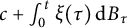and take the expectation to obtain

$$ \begin{align*}\chi_{\xi, c, k}(t)&= \frac{1}{\Gamma(\alpha)}\int^t_0 (t-\tau)^{\alpha-1}(i\lambda^\beta_k \chi_{\xi, c, k}(\tau)- i \kappa_{\xi, c, k}(\tau))\,\mathrm{d}\tau\\&\quad + \frac{-i}{\Gamma(\alpha)}\mathbb{E}[(\int^t_0 (t-\tau)^{\alpha-1}\sigma_k(\tau)\,\mathrm{d}B_\tau)(\int^t_0 \xi(\tau)\,\mathrm{d}B_\tau)]\\& = \frac{1}{\Gamma(\alpha)}\int^t_0 (t-\tau)^{\alpha-1}(i\lambda^\beta_k \chi_{\xi, c, k}(\tau)- i \kappa_{\xi, c, k}(\tau))\,\mathrm{d}\tau\\ &\quad +\frac{-i}{\Gamma(\alpha)}(\int^t_0 (t-\tau)^{\alpha-1}\sigma_k(\tau) \mathbb{E}[\xi(\tau)]\,\mathrm{d}\tau,\end{align*} $$

StartLayout 1st Row 1st Column chi Subscript xi comma c comma k Baseline left parenthesis t right parenthesis 2nd Column equals StartFraction 1 Over normal upper Gamma left parenthesis alpha right parenthesis EndFraction integral Subscript 0 Superscript t Baseline left parenthesis t minus tau right parenthesis Superscript alpha minus 1 Baseline left parenthesis i lamda Subscript k Superscript beta Baseline chi Subscript xi comma c comma k Baseline left parenthesis tau right parenthesis minus i kappa Subscript xi comma c comma k Baseline left parenthesis tau right parenthesis right parenthesis normal d tau 2nd Row 1st Column Blank 2nd Column plus StartFraction negative i Over normal upper Gamma left parenthesis alpha right parenthesis EndFraction double struck upper E left bracket left parenthesis integral Subscript 0 Superscript t Baseline left parenthesis t minus tau right parenthesis Superscript alpha minus 1 Baseline sigma Subscript k Baseline left parenthesis tau right parenthesis normal d upper B Subscript tau Baseline right parenthesis left parenthesis integral Subscript 0 Superscript t Baseline xi left parenthesis tau right parenthesis normal d upper B Subscript tau Baseline right parenthesis right bracket 3rd Row 1st Column Blank 2nd Column equals StartFraction 1 Over normal upper Gamma left parenthesis alpha right parenthesis EndFraction integral Subscript 0 Superscript t Baseline left parenthesis t minus tau right parenthesis Superscript alpha minus 1 Baseline left parenthesis i lamda Subscript k Superscript beta Baseline chi Subscript xi comma c comma k Baseline left parenthesis tau right parenthesis minus i kappa Subscript xi comma c comma k Baseline left parenthesis tau right parenthesis right parenthesis normal d tau 4th Row 1st Column Blank 2nd Column plus StartFraction negative i Over normal upper Gamma left parenthesis alpha right parenthesis EndFraction left parenthesis integral Subscript 0 Superscript t Baseline left parenthesis t minus tau right parenthesis Superscript alpha minus 1 Baseline sigma Subscript k Baseline left parenthesis tau right parenthesis double struck upper E left bracket xi left parenthesis tau right parenthesis right bracket normal d tau comma EndLayout

where the last identity above is ensured by Itô’s isometry (see Lemma 3.1.5 in [Reference Oksendal31]). This implies that $\chi _{\xi , c, k}$ solves the deterministic fractional ODE

(24) $$ \begin{align} \left\{ \begin{aligned} (i\partial_t^\alpha + \lambda^\beta_k) \chi_{\xi, c, k}(t)&= \kappa_{\xi, c, k}(t)+ \sigma_k(t) \mathbb{E}[\xi(t)],\\ \chi_{\xi, c, k}(0)&= 0. \end{aligned} \right. \end{align} $$

On the other hand, we can multiply the expression of $v_k(t)$ by $c+\int ^t_0 \xi (\tau )\,\mathrm {d}B_\tau $ 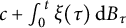. Again we take the expectation and use Itô’s isometry to obtain

$$ \begin{align*}\tilde{\chi}_{\xi, c, k}(t)&= \int^t_0 -i(t-\tau)^{\alpha-1} E_{\alpha, \alpha}(i\lambda^\beta_k (t-\tau)^\alpha)\kappa_{\xi, c, k}(\tau)\,\mathrm{d}\tau\\&\quad +\mathbb{E}[(\int^t_0 -i(t-\tau)^{\alpha-1} E_{\alpha, \alpha}(i\lambda^\beta_k (t-\tau)^\alpha)\sigma_k(\tau)\,\mathrm{d}B_\tau)(\int^t_0 \xi(\tau)\,\mathrm{d}B_\tau)]\\&= \int^t_0 -i(t-\tau)^{\alpha-1} E_{\alpha, \alpha}(i\lambda^\beta_k (t-\tau)^\alpha)\kappa_{\xi, c, k}(\tau)\,\mathrm{d}\tau\\&\quad + \int^t_0 -i(t-\tau)^{\alpha-1} E_{\alpha, \alpha}(i\lambda^\beta_k (t-\tau)^\alpha)\sigma_k(\tau)\mathbb{E}[\xi(\tau)]\,\mathrm{d}\tau.\end{align*} $$

StartLayout 1st Row 1st Column ModifyingAbove chi With tilde Subscript xi comma c comma k Baseline left parenthesis t right parenthesis 2nd Column equals integral Subscript 0 Superscript t Baseline minus i left parenthesis t minus tau right parenthesis Superscript alpha minus 1 Baseline upper E Subscript alpha comma alpha Baseline left parenthesis i lamda Subscript k Superscript beta Baseline left parenthesis t minus tau right parenthesis Superscript alpha Baseline right parenthesis kappa Subscript xi comma c comma k Baseline left parenthesis tau right parenthesis normal d tau 2nd Row 1st Column Blank 2nd Column plus double struck upper E left bracket left parenthesis integral Subscript 0 Superscript t Baseline minus i left parenthesis t minus tau right parenthesis Superscript alpha minus 1 Baseline upper E Subscript alpha comma alpha Baseline left parenthesis i lamda Subscript k Superscript beta Baseline left parenthesis t minus tau right parenthesis Superscript alpha Baseline right parenthesis sigma Subscript k Baseline left parenthesis tau right parenthesis normal d upper B Subscript tau Baseline right parenthesis left parenthesis integral Subscript 0 Superscript t Baseline xi left parenthesis tau right parenthesis normal d upper B Subscript tau Baseline right parenthesis right bracket 3rd Row 1st Column Blank 2nd Column equals integral Subscript 0 Superscript t Baseline minus i left parenthesis t minus tau right parenthesis Superscript alpha minus 1 Baseline upper E Subscript alpha comma alpha Baseline left parenthesis i lamda Subscript k Superscript beta Baseline left parenthesis t minus tau right parenthesis Superscript alpha Baseline right parenthesis kappa Subscript xi comma c comma k Baseline left parenthesis tau right parenthesis normal d tau 4th Row 1st Column Blank 2nd Column plus integral Subscript 0 Superscript t Baseline minus i left parenthesis t minus tau right parenthesis Superscript alpha minus 1 Baseline upper E Subscript alpha comma alpha Baseline left parenthesis i lamda Subscript k Superscript beta Baseline left parenthesis t minus tau right parenthesis Superscript alpha Baseline right parenthesis sigma Subscript k Baseline left parenthesis tau right parenthesis double struck upper E left bracket xi left parenthesis tau right parenthesis right bracket normal d tau period EndLayout

Based on (8), (9), and (11) in Proposition 3.1, we know that $\tilde {\chi }_{\xi , c, k}$ is the solution of (24) as well. Hence, we conclude that ${\chi }_{\xi , c, k}= \tilde {\chi }_{\xi , c, k}$ .

To verify the estimate (19), we use $u^D_k(t)$ and $u^I_k(t)$ to denote the deterministic integral and the Itô integral in (22). Suppose $\mathrm {supp}\,f\cup \mathrm {supp}\,\sigma \subset (0, T_0)\times M$ for some $T_0> 0$ . By Itô’s isometry, the boundedness of $E_{\alpha , \alpha }$ on the imaginary axis and Cauchy–Schwarz inequality, we have

$$ \begin{align*}\mathbb{E}[\,||u(t)||^2_{L^2(M)}\,]&= \sum^\infty_{k=0}\mathbb{E}[|u_k(t)|^2] = \sum^\infty_{k=0}|u^D_k(t)|^2+ \sum^\infty_{k=0}\mathbb{E}[|u^I_k(t)|^2]\\&\leq CT^{2\alpha-1}_0\sum^\infty_{k=0}\int^{T_0}_0|f_k(\tau)|^2\,\mathrm{d}\tau+ \sum^\infty_{k=0}\int^t_0(t- \tau)^{2(\alpha-1)}|E_{\alpha, \alpha}(i\lambda^\beta_k (t-\tau)^\alpha)|^2|\sigma_k(\tau)|^2\,\\&\leq CT^{2\alpha-1}_0\int^{T_0}_0||f(\tau)||^2_{L^2(M)}\,\mathrm{d}\tau+ C'\int^t_0(t- \tau)^{2(\alpha-1)}||\sigma(\tau)||_{L^2(M)}^2\,\mathrm{d}\tau\\&\leq CT^{2\alpha-1}_0\int^{T_0}_0||f(\tau)||^2_{L^2(M)}\,\mathrm{d}\tau+ C"T^{2\alpha-1}_0\sup_t ||\sigma(t)||_{L^2(M)}^2< \infty.\\[-34pt] \end{align*} $$

StartLayout 1st Row 1st Column double struck upper E left bracket StartAbsoluteValue EndAbsoluteValue u left parenthesis t right parenthesis StartAbsoluteValue EndAbsoluteValue Subscript upper L squared left parenthesis upper M right parenthesis Superscript 2 Baseline right bracket 2nd Column equals sigma summation Underscript k equals 0 Overscript infinity Endscripts double struck upper E left bracket StartAbsoluteValue u Subscript k Baseline left parenthesis t right parenthesis EndAbsoluteValue squared right bracket equals sigma summation Underscript k equals 0 Overscript infinity Endscripts StartAbsoluteValue u Subscript k Superscript upper D Baseline left parenthesis t right parenthesis EndAbsoluteValue squared plus sigma summation Underscript k equals 0 Overscript infinity Endscripts double struck upper E left bracket StartAbsoluteValue u Subscript k Superscript upper I Baseline left parenthesis t right parenthesis EndAbsoluteValue squared right bracket 2nd Row 1st Column Blank 2nd Column less than or equals upper C upper T 0 Superscript 2 alpha minus 1 Baseline sigma summation Underscript k equals 0 Overscript infinity Endscripts integral Subscript 0 Superscript upper T 0 Baseline StartAbsoluteValue f Subscript k Baseline left parenthesis tau right parenthesis EndAbsoluteValue squared normal d tau plus sigma summation Underscript k equals 0 Overscript infinity Endscripts integral Subscript 0 Superscript t Baseline left parenthesis t minus tau right parenthesis Superscript 2 left parenthesis alpha minus 1 right parenthesis Baseline StartAbsoluteValue upper E Subscript alpha comma alpha Baseline left parenthesis i lamda Subscript k Superscript beta Baseline left parenthesis t minus tau right parenthesis Superscript alpha Baseline right parenthesis EndAbsoluteValue squared StartAbsoluteValue sigma Subscript k Baseline left parenthesis tau right parenthesis EndAbsoluteValue squared 3rd Row 1st Column Blank 2nd Column less than or equals upper C upper T 0 Superscript 2 alpha minus 1 Baseline integral Subscript 0 Superscript upper T 0 Baseline StartAbsoluteValue EndAbsoluteValue f left parenthesis tau right parenthesis StartAbsoluteValue EndAbsoluteValue Subscript upper L squared left parenthesis upper M right parenthesis Superscript 2 Baseline normal d tau plus upper C prime integral Subscript 0 Superscript t Baseline left parenthesis t minus tau right parenthesis Superscript 2 left parenthesis alpha minus 1 right parenthesis Baseline StartAbsoluteValue EndAbsoluteValue sigma left parenthesis tau right parenthesis StartAbsoluteValue EndAbsoluteValue Subscript upper L squared left parenthesis upper M right parenthesis Superscript 2 Baseline normal d tau 4th Row 1st Column Blank 2nd Column less than or equals upper C upper T 0 Superscript 2 alpha minus 1 Baseline integral Subscript 0 Superscript upper T 0 Baseline StartAbsoluteValue EndAbsoluteValue f left parenthesis tau right parenthesis StartAbsoluteValue EndAbsoluteValue Subscript upper L squared left parenthesis upper M right parenthesis Superscript 2 Baseline normal d tau plus upper C quotation mark upper T 0 Superscript 2 alpha minus 1 Baseline sup Underscript t Endscripts StartAbsoluteValue EndAbsoluteValue sigma left parenthesis t right parenthesis StartAbsoluteValue EndAbsoluteValue Subscript upper L squared left parenthesis upper M right parenthesis Superscript 2 Baseline less than infinity period EndLayout

Note that $\mathbb {E}[u^I_k(t)]= 0$ 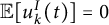so the expectation of the solution of the stochastic problem (18) is exactly the same as the solution of the deterministic problem (1). Hence, we can formulate the inverse problem and state Theorem 1.1 in the following probabilistic way.

For given nonempty open subsets $W_1, W_2 \subset M$ and fixed deterministic deviation function $\sigma $ , we define the source-to-solution map

(25) $$ \begin{align} L^{\alpha, \beta}_{W_1, W_2}: f\to u_f|_{W_2\times (0, \infty)}, \qquad \mathrm{supp} (f)\subset W_1\times (0, \infty), \end{align} $$

where the stochastic function $u_f$ is the solution of (18) corresponding to the mean of the source f.

Theorem 5.3 Suppose $(M, g)$ , $(M, \tilde {g})$ are smooth connected closed Riemannian manifolds. Suppose $1/2< \alpha , \tilde {\alpha }< 1,$ and $\beta , \tilde {\beta }\in (0, 1/2)\cup (1/2, 1)$ . Let $W_1, W_2\subset M$ be nonempty disjoint open subsets. Suppose $W_1$ satisfies the spectral bound condition (5) and $W_2$ has smooth boundary. We fix the deterministic function $\sigma \in C^2_c((0, \infty ); L^2(W_1))$ . Let $L^{\alpha , \beta }_{W_1, W_2}, \tilde {L}^{\tilde {\alpha }, \tilde {\beta }}_{W_1, W_2}$ 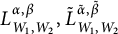be the source-to-solution maps corresponding to $g, \tilde {g}$ . Suppose $g= \tilde {g}$ in $W_1\cup W_2$ and

(26) $$ \begin{align} \mathbb{E}[L^{\alpha, \beta}_{W_1, W_2} f]= \mathbb{E}[\tilde{L}^{\tilde{\alpha}, \tilde{\beta}}_{W_1, W_2} f],\qquad \text{for }f\in C^2_c((0, \infty); L^2(W_1)). \end{align} $$

Then $\alpha = \tilde {\alpha }$ , $\beta = \tilde {\beta }$ , and $(M, g)$ and $(M, \tilde {g})$ are isometric Riemannian manifolds.

Acknowledgements

The author would like to thank Prof. Katya Krupchyk for suggesting the problem and for helpful discussions.

References

Achar, B. N. N., Yale, B. T., and Hanneken, J. W., Time fractional Schrödinger equation revisited . Adv. Math. Phys. 2013(2013), no. 1, 290216.Google Scholar

Anh, P. T., Doan, T. S., and Huong, P. T., A variation of constant formula for Caputo fractional stochastic differential equations . Statist. Probab. Lett. 145(2019), 351–358.Google Scholar

Ashurov, R. R. and Shakarova, M. D., Time-dependent source identification problem for fractional Schrodinger type equations . Lobachevskii J. Math. 43(2022), no. 2, 303–315.Google Scholar

Belishev, M. I. and Kurylev, Y. V., To the reconstruction of a Riemannian manifold via its spectral data (Bc–method) . Comm. Partial Differential Equations 17(1992), nos. 5–6, 767–804.Google Scholar

Cheng, J., Nakagawa, J., Yamamoto, M., and Yamazaki, T., Uniqueness in an inverse problem for a one-dimensional fractional diffusion equation . Inverse Problems 25(2009), no. 11, 115002.Google Scholar

Covi, G., Uniqueness for the fractional Calderón problem with quasilocal perturbations . SIAM J. Math. Anal. 54(2022), no. 6, 6136–6163.Google Scholar

Covi, G., Mönkkönen, K., Railo, J., and Uhlmann, G., The higher order fractional Calderón problem for linear local operators: Uniqueness . Adv. Math. 399(2022), 108246.Google Scholar

Dong, J. and Mingyu, X., Space–time fractional Schrödinger equation with time-independent potentials . J. Math. Anal. Appl. 344(2008), no. 2, 1005–1017.Google Scholar

Feizmohammadi, A., Ghosh, T., Krupchyk, K., and Uhlmann, G., Fractional anisotropic Calderón problem on closed Riemannian manifolds . J. Differential Geom. 131(2025), no. 2, 401–414.Google Scholar

Feizmohammadi, A., Krupchyk, K., and Uhlmann, G., Calderón problem for fractional Schrödinger operators on closed Riemannian manifolds . Inventiones mathematicae 2026, 1–54. Published online, 09 June, 2026.Google Scholar

Feng, X., Li, P., and Wang, X., An inverse potential problem for the stochastic diffusion equation with a multiplicative white noise . Inverse Probl. Imaging 18(2024), no. 1, 271–285.Google Scholar

Ghosh, T., Rüland, A., Salo, M., and Uhlmann, G., Uniqueness and reconstruction for the fractional Calderón problem with a single measurement . J. Funct. Anal. 279(2020), no. 1, 108505.Google Scholar

Ghosh, T., Salo, M., and Uhlmann, G., The Calderón problem for the fractional Schrödinger equation . Anal. PDE 13(2020), no. 2, 455–475.Google Scholar

Gorenflo, R., Kilbas, A. A., Mainardi, F., and Rogosin, S. V., Mittag-Leffler functions, related topics and applications, (Vol. 1451), Berlin: Springer, 2020.Google Scholar

Helin, T., Lassas, M., Oksanen, L., and Saksala, T., Correlation based passive imaging with a white noise source . J. Math. Pures Appl. (9) 116(2018), 132–160.Google Scholar

Helin, T., Lassas, M., Ylinen, L., and Zhang, Z., Inverse problems for heat equation and space–time fractional diffusion equation with one measurement . J. Differential Equations 269(2020), no. 9, 7498–7528.Google Scholar

Hislop, P. D. and Soccorsi, E., Edge currents for the time-fractional, half-plane, Schrödinger equation with constant magnetic field. Journal of Mathematical Physics 65(2024), no. 10, 102101.Google Scholar

Kachalov, A., Kurylev, Y., and Lassas, M., Inverse boundary spectral problems, Chapman and Hall/CRC, Boca Raton, Florida, 2001.Google Scholar

Kian, Y., Li, Z., Liu, Y., and Yamamoto, M., The uniqueness of inverse problems for a fractional equation with a single measurement . Math. Ann. 380(2021), nos. 3–4, 1465–1495.Google Scholar

Krupchyk, K., Kurylev, Y., and Lassas, M., Inverse spectral problems on a closed manifold . J. Math. Pures Appl. (9) 90(2008), no. 1, 42–59.Google Scholar

Lai, R.-Y., Lin, Y.-H., and Rüland, A., The Calderón problem for a space-time fractional parabolic equation . SIAM J. Math. Anal. 52(2020), no. 3, 2655–2688.Google Scholar

Lai, R.-Y. and Zhou, T., An inverse problem for the non-linear fractional magnetic Schrödinger equation . J. Differential Equations 343(2023), 64–89.Google Scholar

Laskin, N., Fractional quantum mechanics . Phys. Rev. E (3) 62(2000), no. 3, 3135.Google Scholar

Laskin, N., Fractional Schrödinger equation . Phys. Rev. E (3) 66(2002), no. 5, 56108.Google Scholar

Lassas, M., Nursultanov, M., Oksanen, L., and Ylinen, L., Disjoint data inverse problem on manifolds with quantum chaos bounds. SIAM Journal on Mathematical Analysis 56(2024), no. 6, 7748–7779.Google Scholar

Lassas, M. and Oksanen, L., Inverse problem for the Riemannian wave equation with Dirichlet data and Neumann data on disjoint sets . Duke Math. J. 163(2014), no. 6, 1071–1103.Google Scholar

Li, L., On inverse problems for uncoupled space-time fractional operators involving time-dependent coefficients . Inverse Probl. Imaging 17(2023), no. 4, 890–906.Google Scholar

Li, L. and Zhang, Y., On inverse problems for a strongly damped wave equation on compact manifolds . J. Geom. Anal. 34(2024), no. 4, 118.Google Scholar

Li, M., Chen, C., and Li, P., Inverse random source scattering for the Helmholtz equation in inhomogeneous media . Inverse Problems 34(2017), no. 1, 15003.Google Scholar

Naber, M., Time fractional Schrödinger equation . J. Math. Phys. 45(2004), no. 8, 3339–3352.Google Scholar

Oksendal, B., Stochastic differential equations: An introduction with applications, Springer Science & Business Media, Berlin, Heidelberg, New York (Springer-Verlag), 2013.Google Scholar

Podlubny, I., Fractional differential equations: An introduction to fractional derivatives, fractional differential equations, to methods of their solution and some of their applications, (Vol. 198). Elsevier, Amsterdam, Netherlands, 1998.Google Scholar

Rüland, A., Unique continuation for fractional Schrödinger equations with rough potentials . Comm. Partial Differential Equations 40(2015), no. 1, 77–114.Google Scholar

Tatar, S. I., Tinaztepe, R., and Ulusoy, S., Simultaneous inversion for the exponents of the fractional time and space derivatives in the space-time fractional diffusion equation . Appl. Anal. 95(2016), no. 1, 1–23.Google Scholar

Article contents

An inverse problem for the space–time fractional Schrödinger equation on closed manifolds

Abstract

Keywords

MSC classification

Information

1 Introduction

1.1 Connection with earlier literature

1.2 Organization

2 Preliminaries

2.1 Laplace–Beltrami operator and Sobolev spaces

2.2 Caputo derivatives and Mittag-Leffler functions

3 Well-posedness

4 Inverse problem

4.1 Determination of the time-fractional power

4.2 Determination of the space-fractional power and the metric

Proposition 4.3 [Reference Lassas, Nursultanov, Oksanen and Ylinen25, Theorem 1.1]

5 Probabilistic formulation

Acknowledgements

References

Save article to Kindle

Save article to Dropbox

Save article to Google Drive

Reply to: Submit a response

Your details

You have entered the maximum number of contributors

Conflicting interests