2. A useful setting

In this paper, for simplicity, we work in the setting of complex-Riemannian manifolds (the ‘real setting’ means that we deal with (complexifications of) real-analytic Riemannian manifolds (note that, semi-Riemannian manifolds could be, also, considered)). For simplicity, we omit the word ‘complex’.

Let $(P,M,G)$ be a principal bundle and let $E$ be a vector bundle over $M$ endowed with a (vector bundles) morphism $\rho :E\to TM$ . Recall [Reference Pantilie15] that, by a $\rho$ -connection on $(P,M,G)$ , we mean a morphism from $E$ to $TP/G$ , which, when composed with the canonical morphism from $TP/G$ to $TM$ , gives $\rho$ .

We are interested in the following setting.

A significant particular case of Remark 1.1 is the following. Let $\mathfrak{g}\subseteq \mathfrak{so}(n+1)$ be a Lie algebra endowed with a faithful orthogonal representation of dimension $n+1$ , and let $\mathfrak{h}=\mathfrak{g}\cap \mathfrak{so}(n)$ , where $\mathfrak{so}(n)\subseteq \mathfrak{so}(n+1)$ is the Lie subalgebra preserving some nondegenerate hyperspace, where $n\in \mathbb{N}\setminus \{0\}$ . Assuming $\mathfrak{g}$ nondegenerate, with respect to the Killing form of $\mathfrak{so}(n+1)$ , and denoting by $\mathfrak{m}$ the orthogonal complement of $\mathfrak{h}$ in $\mathfrak{g}$ , we obtain a reductive decomposition $\mathfrak{g}=\mathfrak{h}\oplus \mathfrak{m}$ .

We, further, assume $\dim \mathfrak{m}=n$ and the representation of $\mathfrak{h}$ on $\mathfrak{m}$ , induced by the adjoint representation of $\mathfrak{g}$ , be (up to some nonzero factor) the given $\mathfrak{h}\subseteq \mathfrak{so}(n)$ . Therefore, there exists a linear embedding $\mathfrak{m}\to \mathfrak{g}\subseteq \mathfrak{so}(n+1)$ , given by

\begin{equation*} x\mapsto \begin{pmatrix} h(x) & \quad x \\ -x^T & \quad 0 \end{pmatrix}, \end{equation*}

for any $x\in \mathfrak{m}$ , where $h:\mathfrak{m}\to \mathfrak{so}(n)$ is a linear map such that $[A,h(x)]=h(Ax)$ , for any $A\in \mathfrak{h}$ and $x\in \mathfrak{m}$ .

Therefore, if $\widetilde {A}=(A,x)\in \mathfrak{g}=\mathfrak{h}\oplus \mathfrak{m}$ , then, as an element of $\mathfrak{so}(n+1)$ ,

\begin{equation*} \widetilde {A}= \begin{pmatrix} A+h(x) & \quad x \\ -x^T & \quad 0 \end{pmatrix}. \end{equation*}

Now, we use Remark 1.1, with $M$ a manifold endowed with an almost $H$ -structure and $E=T(L\setminus 0)/(\mathbb{C}\,\setminus \{0\})$ , where $L$ is a line bundle over $M$ endowed with a connection. In particular, $E=TM\oplus \mathbb{C}$ , and we denote by $\unicode{x1D7D9}$ the section of $E$ corresponding to $(0,1)$ , and by $u$ the nowhere zero function on $M$ such that $u{\unicode{x1D7D9}}$ is given by the infinitesimal generator of the action of $\mathbb{C}\,\setminus \{0\}$ on $L$ .

It follows that any $\rho$ -connection $\widetilde {\nabla }$ on $E$ , where $\rho :E\to TM$ is the projection, corresponds to a $\rho$ -connection $\nabla$ on $TM$ , and a section $\gamma$ of $\textrm {Hom}(E,TM)$ . These are related through the involved section $h$ of $\textrm {Hom}(TM,\textrm {End}(TM))$ , as follows.

(1.1) \begin{equation} \begin{split} \widetilde {\nabla }_XY&=\nabla _XY+h(\gamma (X))Y-\lt \gamma (X),Y\gt {\unicode{x1D7D9}},\\ \widetilde {\nabla }_X{\unicode{x1D7D9}}&=\gamma (X),\\ \widetilde {\nabla }_{{\unicode{x1D7D9}}}X&=\nabla _{{\unicode{x1D7D9}}}X+h(\gamma ({\unicode{x1D7D9}}))X-\lt \gamma ({\unicode{x1D7D9}}),X\gt {\unicode{x1D7D9}},\\ \widetilde {\nabla }_{{\unicode{x1D7D9}}}{\unicode{x1D7D9}}&=\gamma ({\unicode{x1D7D9}}), \end{split} \end{equation}

for any (local) vector fields $X$ and $Y$ on $M$ , where $\lt \cdot,\cdot \gt$ denotes the Riemannian metric on $M$ (and where, for simplicity, we did not mention the compatibilities with the structural groups; for example, $h$ is, in fact, a $1$ -form on $M$ with values in the adjoint bundle of the underlying Riemannian structure on $M$ , which is equivariant with respect to the actions of the adjoint bundle of the almost $H$ -structure on $M$ , where $H$ is the simply-connected Lie group with Lie algebra $\mathfrak{h}$ ).

Proposition 1.2. The torsion $\widetilde {T}$ of $\widetilde {\nabla }$ is given by

\begin{align*} \begin{split} \widetilde {T}(X,Y)&=T(X,Y)+h(\gamma (X))Y-h(\gamma (Y))X+\bigl (u\Omega (X,Y)-\lt \gamma (X),Y\gt +\lt \gamma (Y),X\gt \bigr){\unicode{x1D7D9}},\\ \widetilde {T}(X,{\unicode{x1D7D9}})&=\gamma (X)-\nabla _{{\unicode{x1D7D9}}}X-h(\gamma ({\unicode{x1D7D9}}))X+\bigl (u^{-1}X(u)+\lt \gamma ({\unicode{x1D7D9}}),X\gt \bigr){\unicode{x1D7D9}}, \end{split} \end{align*}

for any $X,Y\in TM$ , where $T$ is the torsion of the connection given by $\nabla$ (and the connection on $L$ ), and $\Omega$ is the curvature form of the connection on $L$ .

Let $G\subseteq O(k)$ be a Lie subgroup and $M$ a Riemannian manifold, $\dim M=k$ , $k\in \mathbb{N}\setminus \{0\}$ . We say that $M$ is a $G$ -manifold if its orthonormal frame bundle admits a reduction $(P,M,G)$ endowed with a connection that gives the Levi-Civita connection of $M$ . Note that, without the connection assumption, we retrieve the basic notion of ‘almost $G$ -structure’.

We consider only nowhere isotropic Killing vector fields $V$ on $G$ -manifolds $M$ which are infinitesimal automorphisms of the given $G$ -structure; that is, their flow preserves the reduction $(P,M,G)$ and its connection. We, further, assume that the frames from $P$ whose first vector is given by $V$ (locally) normalised form a principal bundle preserved by the local flow of $V$ .

Let $\mathbb{C}\,^{m}$ , $(m\in \mathbb{N}\setminus \{0\})$ , be endowed with its canonical Riemannian structure, given by the canonical symmetric bilinear form $\lt \cdot,\cdot \gt$ . The unit sphere, of dimension $m-1$ , is the submanifold of $\mathbb{C}\,^{m}$ formed of those $u\in \mathbb{C}\,^{m}$ such that $\lt u,u\gt =1$ .

Theorem 1.3. Let $M$ be a $G$ -manifold, with $G$ connected and acting transitively on the unit sphere. Let $H\subseteq G$ be the connected Lie subgroup whose Lie algebra is formed of those matrices of the Lie algebra of $G$ whose first rows and columns are zero.

Let $M$ be endowed with a Killing vector field such that $H$ is the structural group of the bundle of frames whose first vector is given by $V$ normalised.

Then, locally, $M$ is of the form $N\times \mathbb{C}\,$ with the metric $\lt \cdot,\cdot \gt +u^2(\textrm {d}t+A)^2$ , where $ (N,\lt \cdot,\cdot \gt\! )$ is an almost $H$ -manifold endowed with a compatible connection $\nabla$ , a section $\mathcal{B}$ of its adjoint bundle, a nowhere zero function $u$ , and a $1$ -form $A$ such that, on denoting by $\gamma$ , the $(1,1)$ -tensor field on $N$ given by $\gamma (X)=\mathcal{B}X-u^{-1}h(\textrm {grad}\,u)X$ , for any $X\in TN$ , the following relations hold

(1.2) \begin{equation} \begin{split} T(X,Y)&=-h(\gamma (X))Y+h(\gamma (Y))X,\\ \textrm {d}A(X,Y)&=2u^{-1}\lt \gamma (X),Y\gt , \end{split} \end{equation}

for any $X,Y\in TN$ , where $T$ is the torsion of $\nabla$ ; in particular, $\nabla +h\circ \gamma$ is the Levi-Civita connection of $ (N,\lt \cdot,\cdot \gt\! )$ .

3. Basic facts in the geometry in dimension $6$

The starting point of this section is the following known fact (see [Reference Chiossi and Salamon6]), where $\mathfrak{g}_2$ is the simple Lie algebra of dimension 14 (see [Reference Pantilie17] for an explicit description and, also, the proof of Proposition 2.1, below).

Proof. We have to show that we are in the setting of Section 2 with $\mathfrak{g}=\mathfrak{g}_2\subseteq \mathfrak{so}(7)$ , and $\mathfrak{sl}(3)=\mathfrak{g}_2\,\cap \,\mathfrak{so}(6)$ .

We choose to deduce this by giving an explicit description, in matrix form, of the Lie algebras embeddings $\mathfrak{sl}(3)\subseteq \mathfrak{g}_2\subseteq \mathfrak{so}(7)$ . For this, if $x\in \mathbb{C}\,^{3}$ , we denote by $[x]$ the element of $\mathfrak{so}(3)$ such that $[x]y=x\times y$ , for any $y\in \mathbb{C}\,^{3}$ , where $\times$ denotes the quaternionic cross product (the well known explicit description of the isomorphism of Lie algebras between $(\mathbb{C}\,^{3},\times)$ and $\mathfrak{so}(3)$ ). Also, we use the characterisation of $\mathfrak{sl}(3)\subseteq \mathfrak{so}(6)$ as formed of all the matrices $\begin{pmatrix} [x] & \quad -y \\ y & \quad [x] \end{pmatrix} ,$ with $x\in \mathbb{C}\,^{3}$ and $y$ a $3\times 3$ trace-free symmetric matrix.

Now, we use the obvious embedding of $\mathfrak{so}(6)$ into $\mathfrak{so}(7)$ whose image has the fourths’ rows and columns equal to zero. Also, we embed $\mathbb{C}\,^{6}$ into $\mathfrak{so}(7)$ as follows: to any $(a,b)\in \mathbb{C}\,^{6}=\mathbb{C}\,^{3}\oplus \mathbb{C}\,^{3}$ , we associate $\{a\}^1+\{b\}^2$ , where

\begin{equation*}\{a\}^1= \begin{pmatrix} 0 &\quad 2a & \quad [a] \\ -2a^T &\quad 0 & \quad 0 \\ [a] & \quad 0 &\quad 0 \end{pmatrix},\ \{b\}^2= \begin{pmatrix} [b] &\quad 0 &\quad 0 \\ 0 &\quad 0 &\quad -2b^T \\ 0 &\quad 2b &\quad -[b] \end{pmatrix} .\end{equation*}

From [Reference Pantilie17], we deduce that $\mathfrak{g}_2$ is, inside $\mathfrak{so}(7)$ , the direct sum of $\mathfrak{sl}(3)$ and $\mathbb{C}\,^{6}$ , and the proof follows.

Let $N$ be a Riemannian manifold of dimension $6$ endowed with a reduction $P$ of its orthonormal frame bundle to $\textrm { GL}(3)$ , corresponding to an almost Hermitian structure $J$ . Similarly to Remark 1.1, the Levi-Civita connection $\nabla$ of $N$ corresponds to a connection on $P$ and a $(1,1)$ -tensor field $A$ on $N$ .

Then $(N,J)$ is nearly-Kähler (that is, $(\nabla _XJ)(X)=0$ , for any $X\in TN$ ) if and only if, pointwisely, $A$ is in the space generated by $\textrm {Id}_{TN}$ and $J$ .

Unless otherwise stated, any nondegenerate hypersurface in an almost $G_2$ -manifold will be considered endowed with the almost Hermitian structure given (up to sign) by the octonionic cross product.

4. Killing vector fields on $\boldsymbol{G}_2$ -manifolds

Approaches different to the one of this section can be found in [Reference Apostolov and Salamon1] and [Reference Fowdar11].

To give an almost $\textrm {SL}(3)$ -structure, through the direct sum of its fundamental representations, on a six-dimensional Riemannian manifold $N$ is the same as to specify the bundle of nondegenerate ‘associative’ spaces contained by $TN$ . Here, associativity is induced by the octonionic cross product on the bundle $E=TN\oplus \mathbb{C}$ , obtained through the setting of Section 2 (and with $M$ replaced by $N$ ), by taking $\mathfrak{g}=\mathfrak{g}_2$ and $\mathfrak{h}=\mathfrak{sl}(3)$ (see, also, Proposition 2.1 whose explicit formulae for the embedding $\mathfrak{sl}(3)\subseteq \mathfrak{g}_2$ require a choice of a nondegenerate associative space).

To make the conditions of Corollary 3.1 more explicit, we endow the tangent bundle of $N$ with an ‘associative (orthogonal) decomposition’ $TN=T^+N\oplus T^-N$ . That is, an orthogonal decomposition such that the horizontal lift of $T^+N$ is nondegenerate and closed under the octonionic cross product.

Then, we can write $\mathcal{B}=\begin{pmatrix} [b] &\quad -B \\ B &\quad [b] \end{pmatrix}$ , where $b$ is a section of $T^+N$ and $B$ is a trace-free self-adjoint section of $\textrm { Hom}(T^+N,T^-N)$ , where we use the orientation preserving isometry between $T^+N$ and $T^-N$ given by the octonionic cross product on $TN\oplus \mathbb{C}\,$ .

Also, we have 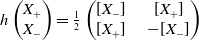$h\begin{pmatrix} X_+\\ X_- \end{pmatrix} =\frac 12\begin{pmatrix} [X_-] &\quad [X_+] \\ [X_+] &\quad -[X_-] \end{pmatrix}$ , for any $X_{\pm }\in T^{\pm }N$ .

Consequently,

(3.1) \begin{equation} \gamma \begin{pmatrix} X_+ \\[2pt] X_- \end{pmatrix} =\begin{pmatrix} b\times X_+ -BX_- -\frac 12\,u^{-1}(\textrm {grad}\,u)_-\times X_+ -\frac 12\,u^{-1}(\textrm {grad}\,u)_+\times X_-\\[2pt] BX_+ +b\times X_- -\frac 12\,u^{-1}(\textrm {grad}\,u)_+\times X_+ +\frac 12\,u^{-1}(\textrm {grad}\, u)_-\times X_- \end{pmatrix}, \end{equation}

for any $X_{\pm }\in T^{\pm }N$ .

Hence, condition (ii) of Corollary 3.1 becomes

(3.2) \begin{equation} \begin{split} \textrm {d}A(X_+,Y_+)&=2u^{-1}\det \bigl (b-\tfrac 12\,u^{-1}(\textrm {grad}\,u)_-,X_+,Y_+\bigr),\\[5pt] \textrm {d}A(X_-,Y_-)&=2u^{-1}\det \bigl (b+\tfrac 12\,u^{-1}(\textrm {grad}\, u)_-,X_-,Y_-\bigr),\\[5pt] \textrm {d}A(X_+,Y_-)&=2u^{-1}\bigl (\lt BX_+,Y_-\gt -\tfrac 12\,u^{-1}\det ((\textrm {grad}\, u)_+,X_+,Y_-)\bigr),\\[5pt] \textrm {d}A(X_-,Y_+)&=2u^{-1}\bigl (-\lt BX_-,Y_+\gt -\tfrac 12\,u^{-1}\det ((\textrm {grad}\, u)_+,X_-,Y_+)\bigr), \end{split} \end{equation}

for any $X_{\pm },Y_{\pm }\in T^{\pm }N$ , where, obviously, the last two equations give the same condition.

Remark 3.3. 1) If $b=\tfrac 12\,u^{-1}(\textrm {grad}\, u)_-$ , $B=0$ , and $(\textrm {grad}\, u)_+=0$ then (3.1) becomes

\begin{equation*}\gamma \begin{pmatrix} X_+ \\ X_- \end{pmatrix} =\begin{pmatrix} 0\\ u^{-1}(\textrm {grad}\,u)_-\times X_- \end{pmatrix},\end{equation*}

for any $X_{\pm }\in T^{\pm }N$ . Therefore, in this case, condition (ii) of Corollary 3.1 becomes

(3.3) \begin{equation} \begin{split} \textrm {d}A(X_-,Y_-)&=2u^{-2}\det ((\textrm {grad}\,u)_-,X_-,Y_-),\\[5pt] \textrm {d}A(X_+,Y_{\pm })&=0, \end{split} \end{equation}

for any $X_{\pm },Y_{\pm }\in T^{\pm }N$ ; equivalently, $\textrm {d}A=2u^{-2}*_-\textrm {d}u$ , where $*_-$ is the Hodge $*$ -operator on $T^-N$ .

Now, we change $\lt \cdot,\cdot \gt$ by the conformal factor $u^2$ along $T^-N$ and by keeping it unchanged elsewhere; denote by $\lt \cdot,\cdot \gt _1$ this new metric on $N$ . Then (3.3) becomes

(3.4) \begin{equation} \textrm {d}A=-*^1_-\textrm {d}(u^{-2}), \end{equation}

where $*^1_-$ is the Hodge $*$ -operator on $T^-N$ , with respect to $\lt \cdot,\cdot \gt _1$ .

If $T^{\pm }N$ are integrable and $\nabla$ is compatible with the decomposition $TN=T^+N\oplus T^-N$ then (i) of Corollary 3.1 holds if and only if the Levi-Civita connection of $\lt \cdot,\cdot \gt _1$ is given by

\begin{equation*}X\mapsto \nabla _X+u^{-1}X(u)\textrm {Id}_{TN}+\tfrac 12\begin{pmatrix} u^{-1}[(\textrm {grad}\,u)_-\times X_-] &\quad 0 \\ 0 &\quad u^{-1}[(\textrm {grad}\,u)_-\times X_-] \end{pmatrix},\end{equation*}

for any $X=X_++X_-\in TN=T^+N\oplus T^-N$ . Consequently, $(N,\lt \cdot,\cdot \gt_1\!)$ is a $\textrm {SL}(3)$ -manifold.

Assume, further, that, up to a suitable (local) frame on $T^+N\,(=T^-N)$ , the local connection form of $\nabla$ is given by the $\mathfrak{so}(3)$ -valued $1$ -form $-\tfrac 12\,u^{-1}[(\textrm {grad}\,u)_-]$ (under the obvious diagonal embedding $\mathfrak{so}(3)\subseteq \mathfrak{sl}(3)$ ). Then, $T^{\pm}N$ are (integrable and) totally geodesic with respect to $\lt \cdot,\cdot \gt$ ; consequently, the same holds for $\lt \cdot,\cdot \gt _1$ . Thus, locally, $(N,\lt \cdot,\cdot \gt _1\!)$ is a product $N^+\times N^-$ , where $N^{\pm }$ are leaves of $T^{\pm }N$ . Then (i) of Corollary 3.1 holds if and only if $N^{\pm }$ are flat. Consequently, by applying Corollary 3.1 we obtain a $G_2$ -manifold which, locally, is a product of a flat Euclidean space of dimension $3$ , and a Ricci-flat anti-self-dual manifold obtained by applying the Gibbons-Hawking construction.

2) If $b=0$ , $B=0$ , and $(\textrm {grad}\,u)_+=0$ (or $(\textrm {grad}\,u)_-=0$ ) then (i) of Corollary 3.1 is equivalent to $(N,u\lt \cdot,\cdot \gt\!)$ is Kähler.

3) If $(\textrm {grad}\,u)_+=0$ (or $(\textrm {grad}\,u)_-=0$ ) then (i) of Corollary 3.1 is equivalent to the fact that the Levi-Civita connection of $(N,u\lt \cdot,\cdot \gt\!)$ is $\nabla ^1+h\circ \mathcal{B}$ , where $\nabla ^1$ is a connection on $N$ compatible with the almost Hermitian structure of $(N,u\lt \cdot,\cdot \gt\!)$ .

The following result can be, also, found in [Reference Apostolov and Salamon1, Proposition 1].

5. Killing vector fields on $\boldsymbol {Spin}(7)$ -manifolds

With the same notations as in Section 2, here, we consider the case $G=\textrm {Spin}(7)$ and $H=G_2$ (compare [Reference Fowdar10]). Then a result similar to Corollary 3.1 follows from Theorem1.3. Furthermore, with $U$ the space of imaginary octonions, $h:U\to \mathfrak{so}(U)$ is given by $h(X)=-\tfrac 13X\times (\!\cdot\!)$ , for any $X\in U$ , where $\times$ denotes the octonionic cross product.

Similarly to Section 4, an orthogonal decomposition $U=U_+\oplus U_-$ with $U_+$ (nondegenerate and) associative, will be called associative.

6. Killing vector fields on special Kähler manifolds

With the same notations as in Section 2, here, we consider the case $G=\textrm {SL}(n)$ and $H=\textrm {SL}(n-1)$ , where the former is considered with the direct sum of its fundamental representations of dimensions $n\geq 2$ . Similarly to the previous sections, these are the eigenspaces of an orthogonal complex structure $J$ on an Euclidean space $\widetilde {U}$ , $\dim \widetilde {U}=2n$ . Furthermore, the induced representation space of $\textrm {SL}(n-1)$ is a codimension $1$ subspace $U\subseteq \widetilde {U}$ admitting an orthogonal decomposition $U=\mathbb{C}\,u_0\oplus U_+\oplus U_-$ , where $u_0\in U$ is such that $\lt u_0,u_0\gt =1$ , $Ju_0\in U^{\perp }$ , and $J|_{U_{\pm }}:U_{\pm }\to U_{\mp }$ are isometries; in particular, $\dim U_{\pm }=n-1$ . Note that $\textrm {SL}(n-1)$ acts trivially on $u_0$ , and ‘canonically’ on $U_+\oplus U_-$ (the latter also holds for $\textrm {SL}(n)$ , with respect to $\widetilde {U}_+=U^{\perp }\oplus U_+$ and $\widetilde {U}_-=\mathbb{C}\,u_0\oplus U_-$ ).

Consequently, the resulting $h:U\to \mathfrak{so}(U)$ is characterised by the following:

(i) $h(u_0)|_{U_+\oplus U_-}=-\tfrac {1}{n-1}J|_{U_+\oplus U_-}$ , $h(u_0)u_0=0$ .

(ii) $h(u_+)u_0=Ju_+$ , $h(u_+)v_+=0$ , $h(u_+)u_-=-\lt Ju_+,u_-\gt u_0$ , for any $u_+,v_+\in U_+$ and $u_-\in U_-$ .

(iii) $h(u_-)u_0=Ju_-$ , $h(u_-)v_-=0$ , $h(u_-)u_+=-\lt Ju_-,u_+\gt u_0$ , for any $u_-,v_-\in U_-$ and $u_+\in U_+$ .