3.1. Preliminary notions

We start by introducing several concepts from the arbitrage theory for semimartingales. Let X be a semimartingale defined on the probability space $(\Omega,(\mathcal{F}_t)_{t\ge 0},\mathbb{P})$ , where the filtration $(\mathcal{F}_t)_{t\ge 0} $ is assumed both right-continuous and complete. This means that

• • for all $t\ge 0$ , $\mathcal F_t = \bigcap_{s>t} \mathcal{F}_s$ ;

• • $\mathcal{F}_0$ contains all $\mathbb{P}$ -negligible events.

We may now define the following objects.

• • A trading strategy is a predictable process $\theta$ with respect to $(\mathcal{F}_t)_{t\ge 0}$ , i.e. for all stopping times $\tau$ , $\theta_{\tau}$ is $\mathcal{F}_{\tau-}$ -measurable.

• • An elementary trading strategy is a trading strategy of the form $\theta_t = \sum_{i=0}^{n}\theta^{(i)}{\mathbf{1}}_{t\in(\tau_{i},\tau_{i+1}]}$ with $n\in\mathbb{N}$ , $(\tau_i)_{i\le n}$ a family of stopping times, and $(\theta^{(i)})_i$ a family of random variables such that, for all i, $\theta^{(i)}$ is $\mathcal{F}_{\tau_i}$ -measurable. Such strategies are also called simple trading strategies.

• • An M-admissible trading strategy, for some $M\ge0$ , is an adapted predictable process $\theta$ with finite variation such that, for all $t\ge0$ , $\int_{0}^{t}\theta_s\,\mathrm{d}X_s>-M$ almost surely (a.s.). An admissible strategy is a strategy that is M-admissible for some $M\ge0$ . We denote the set of all M-admissible strategies by $\mathcal A_M$ .

• • A probability measure $\mathbb{Q}$ is called an equivalent local martingale measure (ELMM) for X if $\mathbb{Q} \sim \mathbb{P}$ and X is a local martingale on $(\Omega,(\mathcal{F}_t)_{t\ge 0},\mathbb{Q})$ .

We now introduce three notions of arbitrage. For more on these, see [Reference Delbaen and Schachermayer24, Reference Karatzas and Kardaras39]. We note that arbitrage notions in a diffusion market with non-trivial interest rates should be expressed in terms of the discounted price process. Otherwise, for the case $r\in \mathbb{R}$ , depending on the sign of r, longing or shorting the riskless asset results in an arbitrage strategy.

The reason we are interested in (NFLVR) is the following result, which qualifies it as a sufficient and necessary condition for the existence of an (ELMM). The latter implies an arbitrage-free pricing framework.

We observe that an arbitrage strategy also realizes a free lunch with vanishing risk. This confirms that (NFLVR) implies (NA). Hence, the following result provides a necessary condition for the existence of an (ELMM).

3.2. The case of the sticky Black–Scholes model

We now study the sticky Black–Scholes model in terms of (NA) and (NFLVR). We first prove that (NFLVR) holds when $r =0$ , by finding an (ELMM) for the discounted price $\widetilde S = S/S^{0}$ . We then prove that (NA), and hence (NFLVR), do not hold when $r \not=0 $ , by establishing an arbitrage strategy.

We first elaborate on the dynamic of the discounted risky asset. From (1) and the Itô formula [Reference Revuz and Yor42, Theorem IV.3.3],

(4) \begin{equation} \mathrm{d}\widetilde S_t = \mathrm{d}({\mathrm{e}}^{-rt}S_t) = {\mathrm{e}}^{-rt}\,\mathrm{d}S_t - r{\mathrm{e}}^{-rt}S_t\,\mathrm{d}t = \big(\mu{\mathbf{1}}_{S_t\not=\zeta}-r\big)\widetilde S_t\,\mathrm{d}t + \sigma\widetilde S_t{\mathbf{1}}_{S_t\not=\zeta}\,\mathrm{d}B_t.\end{equation}

This qualifies $\widetilde S$ as a semimartingale.

The process S is a local martingale under $\mathbb{Q}_x$ as the stochastic integral of a predictable process with respect to a standard Brownian motion. From [Reference Revuz and Yor42, Chapter IV, Corollary 1.25], to prove that S is a martingale it suffices to show that $\mathbb{E}^{\mathbb{Q}_{x}}(\langle S\rangle_t) < \infty$ . Indeed, from (3), we have

\begin{align*} \mathbb{E}^{\mathbb{Q}_{x}}(\langle S\rangle_t) & = \mathbb{E}^{\mathbb{Q}_{x}}\bigg(\int_{0}^{t}\sigma^{2}S^{2}_s{\mathbf{1}}_{S_s\not=\zeta}\,\mathrm{d}s\bigg) \\ & \le \sigma^{2}\int_{0}^{t}\mathbb{E}^{\mathbb{Q}_{x}}\big(S^{2}_s\big)\,\mathrm{d}s \\ & = \sigma^{2}S^{2}_0\int_{0}^{t}\mathbb{E}^{\mathbb{Q}_{x}}\bigg( \exp\bigg({-}\sigma^{2}\int_{0}^{s}{\mathbf{1}}_{S_u\ne\zeta'}\,\mathrm{d}u + 2\sigma\int_{0}^{s}{\mathbf{1}}_{S_u\ne\zeta'}\,\mathrm{d}B_u\bigg)\bigg)\,\mathrm{d}s, \end{align*}

where, from [Reference Revuz and Yor42, Corollary VIII.1.16], the quantity under the expectancy is a martingale. Hence, for all $t\ge 0$ , $\mathbb{E}^{\mathbb{Q}_{x}}(\langle S\rangle_t) \le \sigma^{2}S^{2}_0t$ , which is finite. This proves (iii), which completes the proof.

We consider the trading strategy H defined by

(7) \begin{equation} H_t = \textrm{sgn}({-}r){\mathrm{e}}^{rt}{\mathbf{1}}_{S_t=\zeta}, \quad t>0. \end{equation}

We now show that, for all $t\ge 0$ , $\int_{0}^{t}H_s\,\mathrm{d}\widetilde S_s \ge 0$ , and that there exists some $t>0$ such that $\mathbb{P}\big(\int_{0}^{t}H_s\,\mathrm{d}\widetilde S_s>0\big)>0$ . From (1), (4), and (7),

\begin{equation*} \int_{0}^{t}H_s\,\mathrm{d}\widetilde S_s = \int_{0}^{t}H_s{\mathbf{1}}_{S_s=\zeta}\,\mathrm{d}\widetilde S_s = -r\zeta\int_{0}^{t}H_s{\mathrm{e}}^{-rs}{\mathbf{1}}_{S_s=\zeta}\,\mathrm{d}s = |r|\zeta\int_{0}^{t}{\mathbf{1}}_{S_s=\zeta}\,\mathrm{d}s = |r|\rho\zeta L^{0}_{t}(S). \end{equation*}

We observe that, for all $t\ge 0$ , $\int_{0}^{t}H_s\,\mathrm{d}\widetilde S_s \ge 0$ , i.e. $H\in\mathcal A_0$ . From [Reference Kallenberg38, Corollary 29.18] and [Reference Bruggeman and Ruf15, Theorem 1.1], $\mathbb{P}_x\big(\int_{0}^{t}H_s\,\mathrm{d}\widetilde S_s > 0\big) = \mathbb{P}_x(L^{0}_{t}(S) > 0) = \mathbb{P}_x(\inf\{s>0\colon S_s = \zeta\} < t) > 0$ . These qualify H as an arbitrage strategy. This completes the proof.

Example 2. (Standard Black–Scholes ( $\rho=0$ ); continuation of Example 1 .) In the standard Black–Scholes model the discounted price process has dynamic $\mathrm{d}\widetilde S_t = (\mu-r)\widetilde S_t\,\mathrm{d}t + \sigma\widetilde S_t\,\mathrm{d}B_t$ . An (ELMM) for $\widetilde S$ is the measure $\mathbb{Q}_x$ defined by $\mathrm{d}\mathbb{Q}_x = \mathcal{E}(\theta)_T\,\mathrm{d}\mathbb{P}_x$ , where

\begin{equation*} \mathcal{E}(\theta)_T = \exp\bigg(\int_{0}^{T}\frac{\mu-r}{\sigma}\,\mathrm{d}B_s - \frac{1}{2}\int_{0}^{T}\bigg(\frac{\mu-r}{\sigma}\bigg)^{2}\,\mathrm{d}s\bigg). \end{equation*}

Hence, (NFLVR) is satisfied.

We note also that in the standard Black–Scholes model, if $A+M$ is the Doob–Meyer decomposition of the discounted price process $\widetilde S$ , then $\mathrm{d}A_t \ll \mathrm{d}\langle M\rangle_t$ . Indeed, for all $t\ge 0$ ,

\begin{equation*} A_t = \int_{0}^{t}(\mu-r)\widetilde S_s\,\mathrm{d}s, \qquad M_t = \int_{0}^{t}\sigma\widetilde S_s\,\mathrm{d}B_s. \end{equation*}

Remark 3. In the sticky Black–Scholes model ( $\rho>0$ ), there is no uniqueness of (ELMM) for S. Indeed, we observe that taking any $\theta$ in (5) such that, for all $t \ge 0$ ,

\begin{equation*} \int_{0}^{t}\theta_s{\mathbf{1}}_{S_s\not=\zeta}\,\mathrm{d}s = \int_{0}^{t}\frac{\mu}{\sigma}{\mathbf{1}}_{S_s\not=\zeta}\,\mathrm{d}s, \end{equation*}

also results in an equivalent local martingale measure $\mathbb{Q}^{\theta}$ for S. In this case, the process S solves

\begin{equation*} \begin{cases} \mathrm{d}S_t = \sigma S_t{\mathbf{1}}_{S_t\ne\zeta}\,\mathrm{d}B^{\theta}_t, \\ {\mathbf{1}}_{S_t=\zeta}\,\mathrm{d}t = \rho\,\mathrm{d}L^{\zeta}_{t}(S), \end{cases} \end{equation*}

where $\widetilde B^{\theta} = (B_t-\int_{0}^{t}\theta_s\,\mathrm{d}s)_{t\ge 0}$ is a $\mathbb{Q}^{\theta}$ -Brownian motion.

4.1. Pricing equation

We consider the generic pricing problem

(8) \begin{equation} \begin{cases} v_{t} = -\frac{\sigma^{2}x^{2}}{2}v_{xx} \quad \text{for all } (t,x)\in[0,T)\times(0,\infty), \\ \frac{\sigma^{2}\zeta^{2}}{2}v_{xx}(t,\zeta{-}) = \frac{\sigma^{2}\zeta^{2}}{2}v_{xx}(t,\zeta{+}) = \frac{1}{2\rho}(v_{x}(t,\zeta{+})-v_{x}(t,\zeta{-})) \quad \text{for all } t \in [0,T), \\ v(T,x) = h(x) \quad \text{for all } x \in (0,\infty). \end{cases}\end{equation}

We now define the space of classical solutions of (8). This is justified by Remark 6.

For I an interval of $[0,\infty)$ and L an interval of $(0,\infty)$ , we consider the spaces $C^{L}(I)$ and $C^{1,L}(I\times L)$ defined by

\begin{align*} C^{L}(L) & \,:\!=\, \bigg\{f \in C(L) \cap C^{2}(L)\colon\frac{\sigma^{2}\zeta^{2}}{2}f''(\zeta{-}) = \frac{\sigma^{2}\zeta^{2}}{2}f''(\zeta{-}) = \frac{1}{2\rho}(f'(\zeta{+})-f'(\zeta{-}))\bigg\}, \\ C^{1,L}(I \times L) & \,:\!=\, \big\{u \in C(I \times L)\colon\text{for all } x \in L,\,u(\cdot,x) \in C^{1}(I); \text{ for all } t \in I,\,u(t,\cdot) \in C^{L}(L)\big\},\end{align*}

where all the derivatives considered are right derivatives. We can now define the notion of a classical solution of (8).

We note that the space $C^{L}((0,\infty))$ is comprised of functions that are differences of convex functions. Indeed, if $f \in C^{L}((0,\infty))$ , the function $\phi$ defined by

\begin{equation*} \phi(x) = f(x) - \frac{\rho(\zeta\sigma)^{2}}{2}f''(\zeta)(x - \zeta)_+, \quad x \in (0,\infty),\end{equation*}

is $C^{2}((0,\infty))$ . It suffices to observe that the regularity of $\phi$ ensures it is difference of convex functions, and that $[x \rightarrow (x - \zeta)_+]$ is convex. This justifies the use of the Itô–Tanaka formula [Reference Revuz and Yor42, Theorem VI.1.5] on any $f\in C^{L}((0,\infty))$ .

Proof. Let v be the unique classical solution of (8). Since, for all $t\in [0,T)$ , $v(t,\cdot)\in C^{L}((0,\infty))$ , from the Itô–Tanaka formula,

\begin{align*} \mathrm{d}v(t,S_t) & = v_t(t,S_t)\,\mathrm{d}t + v_x(t,S_t)\,\mathrm{d}S_t \\ & \quad + \frac{1}{2}v_{xx}(t,S_t)\,\mathrm{d}\langle S\rangle_t + \frac{1}{2}(v_{x}(t,\zeta{+}) - v_{x}(t,\zeta{-}))\,\mathrm{d}L^{\zeta}_{t}(S). \end{align*}

From (6), $\mathrm{d}\langle S\rangle_t = \sigma^{2}S^{2}_t{\mathbf{1}}_{S_t\not=\zeta}\,\mathrm{d}t$ and ${\mathbf{1}}_{S_t=\zeta}\,\mathrm{d}t = \rho\,\mathrm{d}L^{\zeta}_{t}(S)$ . This, combined with (8), yields

\begin{equation*} \frac{1}{2}(v_{x}(t,\zeta{+}) - v_{x}(t,\zeta{-}))\,\mathrm{d}L^{\zeta}_{t}(S) = \frac{\rho\sigma^{2}\zeta^{2}}{4}v_{xx}(t,\zeta)\,\mathrm{d}L^{\zeta}_{t}(S) = -v_t(t,\zeta){\mathbf{1}}_{S_t=\zeta}\,\mathrm{d}t. \end{equation*}

Consequently,

\begin{align*} \mathrm{d}v(t,S_t) & = v_t(t,S_t){\mathbf{1}}_{S_t\not=\zeta}\,\mathrm{d}t + v_x(t,S_t)\,\mathrm{d}S_t + \frac{\sigma^{2}S^{2}_t}{2}v_{xx}(t,S_t){\mathbf{1}}_{S_t\not=\zeta}\,\mathrm{d}t \\ & \quad + v_t(t,S_t){\mathbf{1}}_{S_t=\zeta}\,\mathrm{d}t + \frac{1}{2}(v_{x}(t,\zeta{+}) - v_{x}(t,\zeta{-}))\,\mathrm{d}L^{\zeta}_{t}(S) \\ & = v_x(t,S_t)\,\mathrm{d}S_t + \bigg(v_t(t,S_t) + \frac{\sigma^{2}S^{2}_t}{2}v_{xx}(t,S_t)\bigg){\mathbf{1}}_{S_t\not=\zeta}\,\mathrm{d}t. \end{align*}

Integrating in time yields $h(S_T) = v(t,S_t) + \int_{t}^{T}v_x(t,S_s)\,\mathrm{d}S_s$ . This proves the two assertions.

For our next remark, we recall some notation. The semi-group of a diffusion is the family of operators $(P_t)_{t\ge 0}$ defined by $P_t f(x) \,:\!=\, \mathbb{E}(f(S_t) \mid S_0 = x)$ for all $f \in C_{\mathrm{b}}((0,\infty))$ , $t\ge 0$ , $x\in(0,\infty)$ . We note that S is a Feller process [Reference Criens19, Theorem 1], i.e. it is strong Markov and its semi-group $(P_t)_{t\ge 0}$ is internal on $C_0((0,\infty))$ and continuous at 0, i.e.

• • for all $f \in C_0((0,\infty))$ , $P_t f \in C_0((0,\infty))$ ;

• • for all $f \in C_0((0,\infty))$ and $x\in (0,\infty)$ , $\lim_{t\rightarrow 0}P_t f(x) = f(x)$ .

Its semi-group is therefore generated by the operator

\begin{equation*} L f = \frac{(x\sigma)^{2}}{2}f'', \quad \mathrm{dom}_{C_0}(L) = C_0((0,\infty)) \cap C^{L}((0,\infty)).\end{equation*}

4.2. Representation

In Remark 6, we observed that if $h\in \textrm{dom}_{C_0}(L)$ , then the pricing equation has a unique classical solution, the price function has a representation in terms of an expectancy, and a replication strategy exists. In this section we prove that the two latter assertions are part of a more general principle, which is a consequence of the martingale representation property [Reference Criens and Urusov21, Theorem 2.7].

Our motivation is that the condition $h\in \mathrm{dom}_{C_0}(L) $ is quite restrictive. Indeed, classical claims like calls and puts have payoff functions that are neither in $C_0((0,\infty)) $ nor in $C^{L}((0,\infty))$ . This holds true even for the standard Black–Scholes model, where $\mathrm{dom}_{C_0}(L) = C_0((0,\infty)) \cap C^{2}((0,\infty))$ . Nevertheless, as depicted in Section 6.1, we obtain satisfactory numerical results for a call payoff in the sticky and the non-sticky model.

Regarding (ii), from the (APP) (see Definition 4) and the payoff replication relations (9), the price of the claim at t is necessarily $\mathbb{E}^{\mathbb{Q}_x}(h(S_T) \mid \mathcal{F}_t)$ . Any other value would result in an arbitrage opportunity for one of the two parties. This completes the proof.

Remark 7. We note that in the sticky Black–Scholes model ( $\rho>0$ ) we have no uniqueness of the payoff replication strategy. Indeed, let $\delta$ be a payoff replication strategy and $\delta'$ a strategy such that $\delta \not= \delta'$ and, for all $t\ge 0$ , $\delta_t{\mathbf{1}}_{S_t\not=\zeta} = \delta'_t{\mathbf{1}}_{S_t\not=\zeta}$ . Then, we have

\begin{equation*} \mathbb{E}^{\mathbb{Q}_x}(h(S_T) \mid \mathcal{F}_t) - \mathbb{E}^{\mathbb{Q}_x}(h(S_T)) = \int_{0}^{t}\delta_s\,\mathrm{d}S_s = \int_{0}^{t}\delta'_s\,\mathrm{d}S_s. \end{equation*}

Example 3. (Standard Black–Scholes ( $\rho=0$ ); continuation of Examples 1 and 2 .) For the standard Black–Scholes model $(\rho = 0)$ , the risky asset and discounted risky asset price dynamics $S,\widetilde S$ under $\mathbb{Q}_x$ are $\mathrm{d}S_t = S_t(r\,\mathrm{d}t + \sigma\,\mathrm{d}B_t)$ and $\mathrm{d}\widetilde S_t = \sigma\widetilde S_t\,\mathrm{d}B_t$ . The pricing equation [Reference Shreve47, Theorems 6.4.3 and 7.3.1] is

(10) \begin{equation} \begin{cases} v_t(t,x) + rxv_x(t,x) + \frac{\sigma^{2}x^{2}}{2}v_{xx}(t,x) = rv(t,x) & \text{for all } (t,x) \in (0,T)\times (0,\infty), \\ v(T,x) = h(x). \end{cases} \end{equation}

If $h\in \mathsf H(S_T)$ , there exists a replication strategy in $L^{2}$ and the price at $t\in [0,T]$ of the contingent claim of payoff at maturity $h(S_T)$ is given by $V_t \,:\!=\, \mathbb{E}^{\mathbb{Q}_x}({\mathrm{e}}^{-r(T-t)}h(S_T) \mid \mathcal{F}_t)$ . If (10) has a unique classical solution v, the (APP) price of the contingent claim at $t\in[0,T]$ is $V_t = v(t,S_t)$ , and the replication strategy is the process $\delta$ defined [Reference Shreve47, Remark 7.3.3] by $\delta_t \,:\!=\, v_x(t,S_t)$ , $t\in [0,T]$ .

6.1. Hedging time granularity

The message of the Black–Scholes model is as follows: it is possible to replicate the payoff of a European option using a self-financing portfolio composed of quantities of the risky and non-risky assets. In particular, the option seller can hedge their risk by holding a portfolio that, at each time t, comprises $\delta_t = v_x(t,S_t)$ parts of the risky asset.

However, a practical challenge arises since achieving this requires continuous rebalancing of the portfolio composition over time. This, as mentioned in [Reference Bertsimas, Kogan and Lo10], proves impossible in real-world scenarios as it necessitates an infinite number of operations. One way to address this is to introduce a hedging window $h>0$ , resulting in hedging times $(t_{i})_i$ such that $t_{i+1}-t_{i} = h$ . The agent can then rebalance the portfolio at each time $t_i$ so that, for all i, they hold $v_{x}(t_i,S_{t_i})$ parts of the risky asset on $[t_i,t_{i+1})$ . The resulting discretized version of the continuous-time hedging strategy $\delta$ is the strategy $\delta^{(N)}$ defined for all t by $\delta^{(N)}_t = \delta_{[Nt]/N}$ , where $[x]=\sup\{k\in\mathbb{N}\colon k \le x\}$ .

The profits and losses (PnLs) at t of the strategies $\delta$ and $\delta^{(N)}$ are

\begin{equation*} V_t(\delta) - V_0(\delta) = \int_{0}^{t}\delta_s\,\mathrm{d}S_s, \qquad V_t(\delta^{(N)}) - V_0(\delta) = \int_{0}^{t}\delta^{(N)}_s\,\mathrm{d}S_s,\end{equation*}

where, from Theorem 5, the option premium is $V_0(\delta)=\mathbb{E}^{\mathbb{Q}}(h(S_T))$ and $V_t(\delta)=\mathbb{E}^{\mathbb{Q}}(h(S_T)\mid \mathcal{F}_t)$ $= Q^{S,\mathbb{Q}}_{S_t}(h(Y_{T-t}))$ .

This discrete replication strategy, outlined in Algorithm 1, results in replication errors known as the tracking error, defined by $\varepsilon^{(N)}_t \,:\!=\, V_{t}(\delta^{(N)})-V_t(\delta)$ . In [Reference Bertsimas, Kogan and Lo10], the metric used to assess the replication quality is the mean squared tracking error, defined by

\begin{equation*} \mathsf R_T^{(N)} \,:\!=\, \sqrt{\mathbb{E}^{\mathbb{Q}} \big[\big(\varepsilon^{(N)}_T\big)^{2}\big]}.\end{equation*}

Instead of this, we will quantify the replication properties of each model with the pair $\big(\mathbb{E}^{\mathbb{Q}}\big[\varepsilon^{(N)}_t\big],\big(\mathrm{Var}^{\mathbb{Q}}\big[\varepsilon^{(N)}_t\big]\big)^{1/2}\big)$ , where $\mathbb{E}^{\mathbb{Q}}\big[\varepsilon^{(N)}_t\big]$ is the expected replication PnL, with the replication PnL standard deviation being $\big(\mathrm{Var}^{\mathbb{Q}}\big[\varepsilon^{(N)}_t\big]\big)^{1/2}$ . The reason is that $\mathsf R_t^{(N)}$ is more adapted to the case where $\mathbb{E}^{\mathbb{Q}}\big[\varepsilon^{(N)}_t\big]=0$ . If an agent is unsure about the pricing/replication model they apply, they are likely to miscalculate the option premium and end up with non-zero PnL, making the metric $\mathsf R_t^{(N)}$ irrelevant. This is the object of Section 6.2. Another reason for this choice is that the pair $\big(\mathbb{E}^{\mathbb{Q}}\big[\varepsilon^{(N)}_t\big],\big(\mathrm{Var}^{\mathbb{Q}}\big[\varepsilon^{(N)}_t\big]\big)^{1/2}\big)$ contains the information in $\mathsf R_t^{(N)}$ . Indeed, the three quantities are linked by the relation $\mathrm{Var}^{\mathbb{Q}}\big[\varepsilon^{(N)}_t\big] = \big(\mathsf R_t^{(N)}\big)^{2} -\big(\mathbb{E}^{\mathbb{Q}}\big[\varepsilon^{(N)}_t\big]\big)^{2}$ .

We assess the discrete-time hedging error of the sticky Black–Scholes model as follows. We sample trajectories of the sticky geometric Brownian motion. Then, we apply Algorithm 1 to hedge a call option for various hedging windows. Last, we compute the empiric mean and standard deviation of the PnL with

\begin{equation*} \widehat\mu^{(N)}_{\textrm{MC}} = \frac{1}{N_{\textrm{MC}}}\sum_{i=1}^{N_{\textrm{MC}}}\varepsilon^{(N)}_{T}(\omega_i), \qquad \widehat{\sigma}^{(N)}_{\textrm{MC}} = \frac{1}{\sqrt{N_{\textrm{MC}}}\,} \sqrt{\sum_{i=1}^{N_{\textrm{MC}}}\big(\varepsilon^{(N)}_{T}(\omega_i) - \widehat\mu_{\textrm{MC}}\big)^{2}}.\end{equation*}

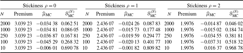
We have no closed-form expressions for the replication strategy and the (APP) prices of claims in the sticky Black–Scholes model. Therefore, we use a finite-difference approximation to numerically solve (8). The simulation results are summarized in Table 1.

Table 1.

Premiums and Monte Carlo estimation of the expected replication error (1000 simulated trajectories) for a call $(K,T)=(10,10)$ for various stickiness and hedging windows. $N_{\textrm{MC}}=1000$ .

From the numerical simulations, we observe the following. The replication errors in the sticky and non-sticky models decreases the higher the hedging frequency N is. Convergence in the sticky model seems to occur at the same rate as for the non-sticky one (standard Black–Scholes model). In [Reference Bertsimas, Kogan and Lo10], it is proved that the rate of convergence for the Black–Scholes model is $\mathcal O(N^{-1/2})$ .

Also, higher stickiness leads to higher tracking errors for coarse hedging time-windows. We attribute this behavior to the inherent discontinuity of the delta function at the sticky threshold. As depicted in Figure 2, higher stickiness at $\zeta$ corresponds to more substantial jumps in the delta, resulting in sudden shifts in portfolio composition whenever the price process S crosses the sticky threshold. Consequently, the discrete-time hedging portfolio manifests substantial deviations in portfolio composition from the ideal configuration whenever the price crosses the sticky threshold. This is illustrated in Figure 3, where spikes and oscillations in the portfolio composition for fine-grained hedging do not appear in coarser regimes.

Figure 2.

Finite difference approximations of the price (left) and delta (right) curves for a call option with strike $K = 11$ and maturity $T = 10$ . The graphs compare prices and deltas for three models: the standard Black–Scholes model with $(r,\sigma) = (0,0.25)$ (solid curves); the sticky Black–Scholes model with $(r,\sigma,\rho,\zeta) = (0,0.25,1.0,10.0)$ (dot-dashed curves); and the sticky Black–Scholes model with $(r,\sigma,\rho,\zeta) = (0,0.25,2.0,10.0)$ (dashed curves).

Figure 3.

(Top): Parts of the risky asset in the payoff replication strategy for one sample path of S with $\rho=0$ , for (black) $N=100$ and (gray) $N=2000$ . (Bottom): Same, but with $\rho=1$ .

6.2. Model mismatch: Constant volatility

Now let’s assume that an agent intends to hedge a contingent claim on an underlying asset with a sticky geometric Brownian motion price dynamic with parameters $(\sigma,\rho,\zeta)$ . The agent considers the following models:

• • Model 1: the standard Black–Scholes model with volatility $\sigma$ .

• • Model 2: the standard Black–Scholes model with volatility $\Sigma_n(X)$ , where for some $T'>0$ , $\Sigma_n(X)$ is the estimator of the realized volatility on $[-T',0)$ of the current sample path. The estimator is defined by

  \begin{equation*} \Sigma_n(X) = \frac{1}{\sqrt{T'}\,}\sqrt{\sum_{i=1}^{[nT']}(\log S_{-{i}/{n}} - \log S_{-({i+1})/{n}})^{2}}. \end{equation*}

• • Model 3: the sticky Black–Scholes model with parameters $(\sigma,\rho,\zeta)$ .

According to Theorem 5, the replication cost for the claim with payoff $h(S_T)$ is $\mathbb{E}^{\mathbb{Q}}[h(S_T)]$ . This matches the (APP) price or premium in Model 3, i.e.,

\begin{equation*} \mathrm{({APP})}\text{ price} = (\text{Premium in Model 3}) = \mathbb{E}^{\mathbb{Q}}[h(S_T)].\end{equation*}

Therefore, the premium is miscalculated in Models 1 and 2. To address the premium miscalculation in each model, we introduce the mispricing error, defined as

\begin{equation*} \epsilon_{\mathrm{MP}} \,:\!=\, (\text{Premium in Model }i) - \mathrm{({APP})}\text{ price}.\end{equation*}

This error compensates for the error made by the agent when using an incorrect model to compute premiums for contingent claims. It is to be compared with the empiric mean PnL of the replication portfolios $\widehat\mu_{\textrm{MC}}$ . The discrepency between values of Model 1 and Model 3 when $\rho=0$ is due to the error incurred from the finite-difference approximations of quantities in Model 3.

We observe in Model 1 that the mispricing error $\epsilon_{\mathrm{MP}}$ is close to the empiric mean PnL of the replication portfolios $\widehat\mu_{\textrm{MC}}$ . This is due to two facts. First, the agent ultimately holds $h(S_T)$ at maturity. Second, given that the price dynamics are martingales on $(\Omega,(\mathcal{F}_t)_{t\ge 0},\mathbb{Q})$ , from (9) the self-financing portfolio is also a martingale. Hence, the expected PnL of any self-financing portfolio is 0 and the expected PnL of the option seller is $\text{Premium} - \mathbb{E}^{\mathbb{Q}}[h(S_T)]$ , which equals 0 only when pricing with the correct model, Model 3. Also, among Models 1, 2, and 3, it is Model 3 that exhibits the lowest hedging error, indicating superior replication properties (see Table 2).

Table 2.

Theoretical premiums in each model, (APP) prices, mean PnLs, and tracking errors for a call $(K,T)=(10,10)$ on assets with price processes $\sigma=0.25$ sticky at $\zeta=10$ for various degrees of stickiness $\rho$ in each model. The hedging frequency is $N=2000$ and the number of simulated sample paths of each process is $N_{\textrm{MC}}=1000$ .

6.3. Model mismatch: Smooth SDE

We now suppose the agent misrepresents price stickiness as local volatility in a smooth SDE model.

It is possible to approximate in law diffusions with sticky features by smooth diffusions. Let X be the diffusion on $(0,\infty)$ , on a natural scale, of speed measure

\begin{equation*} m(dx) = \frac{2}{\sigma^{2}x^{2}}\,\mathrm{d}x + \rho\delta_{\zeta}(dx), \quad x>0.\end{equation*}

It corresponds to the law of S under $\mathbb{Q}$ , see (6). We can define an approximating sequence $(X^{n})_n$ of S in law as follows. For all n, let $X^{n}$ solve $\mathrm{d}X^{n}_t = \sigma_n(X^{n}_t)\,\mathrm{d}B^{n}_t$ with $B^{n}$ a standard Brownian motion and $\sigma_n$ a smooth function, such that

\begin{equation*} \frac{2}{\sigma_{n}^{2}(x)}\,\mathrm{d}x \xrightarrow[n\rightarrow\infty]{\text{weakly}} m(\text{d}x).\end{equation*}

From [Reference Brooks and Chacon14], $X^{n} \rightarrow X$ in law.

We make two key observations. First, the prices in the smooth models converge to the prices in the sticky model. Indeed, let v be the price function and $(Q_{x}^{X})_x$ the Markovian family of the sticky model X, and, for all $n\in \mathbb{N}$ , let $v^{(n)}$ be the price function and $(Q_{x}^{X^{n}})_x$ the Markovian family of the smooth model $X^{n}$ . The convergence in law implies that

\begin{equation*} \lim_{n\rightarrow\infty}v^{(n)}(t,x) = \lim_{n\rightarrow\infty}Q^{X^{n}}_x(h(Y_{T-t})) = Q^{X}_x(h(Y_{T-t})) = v(t,x),\end{equation*}

where Y is the coordinate process. Second, while the deltas in the smooth models are continuous, the delta of the sticky model is discontinuous (see Remark 5). Indeed, due to the smoothness of the coefficient $\sigma_n$ , the function $x \rightarrow v^{(n)}(t,x)$ is also smooth, for all $t\in [0,T] $ and $n\in \mathbb{N}$ .

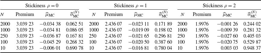
In Section 6.1, we approximated the delta function using an interpolation of the finite-difference scheme that preserved the discontinuity. In this section, we use an approximation that does not preserve the discontinuity. Thus, the deltas for the two approximations differ only locally around the threshold of stickiness. We observe that the second method produces a high tracking error (see Table 3, and compare with Table 1). This indicates that hedging a sticky diffusion using a smooth model results in some significant irreductible tracking error. The reason is that a smooth function of the spot price cannot replicate the discontinuity of the true sticky hedging strategy.

Table 3.

As Table 1 but for the locally linearly interpolated price curve around $\zeta$ .