1 Introduction
Thin liquid films appear in a wide variety of applications, ranging from large-scale geophysical flows, such as lava flows, to small-scale microfluidic devices, such as lab-on-chip technology (see Oron, Davis & Bankoff Reference Oron, Davis and Bankoff1997; Toner & Irimia Reference Toner and Irimia2005; Craster & Matar Reference Craster and Matar2009; SooHoo & Walker Reference SooHoo and Walker2009). In the present study, we consider pressure-driven two-layer flows through channels of variable cross-section that are additionally influenced by the presence of electric fields arising from imposing a constant voltage potential across the channel walls. Sufficiently strong electric fields can destabilise the flow and lead to nonlinear free surface patterns that can be useful in applications, e.g. microlithography. The reader is referred to Melcher & Taylor (Reference Melcher and Taylor1969) and Saville (Reference Saville1997) for general reviews of electrohydrodynamics.
In recent years there has been growing interest in the miniaturisation of electronic tools, and much research has gone into finding appropriate techniques to pattern polymers. Details on the applications and techniques of polymer patterning can be found in the review by Nie & Kumacheva (Reference Nie and Kumacheva2008). One such technique exploits the electrohydrodynamic instabilities of a system to induce ordered patterns, and it was first explored in two experimental papers contemporary with each other (see Chou & Zhuang Reference Chou and Zhuang1999; Schaffer et al. Reference Schaffer, Thurn-Albrecht, Russell and Steiner2000). Since then, electrohydrodynamic instability-induced structures have been the focus of much research due to the simplicity and the low cost of this patterning method, details of which can be found in the review by Wu & Russell (Reference Wu and Russell2009). Linear stability analyses have been conducted using both the perfect dielectric (Schaffer et al. Reference Schaffer, Thurn-Albrecht, Russell and Steiner2001) and the leaky dielectric (Pease & Russell Reference Pease and Russell2002) models. Both predict experimental data reasonably well, with the leaky dielectric decreasing pillar spacing and increasing their rate of formation.
Linear stability analyses and full numerical simulations have been done for a variety of similar set-ups. Ozen et al. (Reference Ozen, Aubry, Papageorgiou and Petropoulos2006) and Li et al. (Reference Li, Ozen, Aubry, Papageorgiou and Petropoulos2007) considered the linear stability of the interface between two conducting fluids bounded by two flat electrodes at arbitrary Reynolds numbers, and found that the electric field has a destabilising effect for perfect dielectrics, and either a stabilising or destabilising effect for leaky dielectrics with either Couette or Poiseuille base flows. A comparison of the instabilities observed when a horizontal or vertical electric field is acting was carried out by Uguz & Aubry (Reference Uguz and Aubry2008) for inertialess flows, and horizontal fields were shown to be stabilising while vertical ones lead to long-wave instabilities. Craster & Matar (Reference Craster and Matar2005) carried out numerical simulations for a two-fluid system under a vertical electric field in the absence of flow, and showed that initially small perturbations developed into spatially periodic columnar structures. Thaokar & Kumaran (Reference Thaokar and Kumaran2005) considered electrified two-fluid Couette flows of equal viscosities at zero Reynolds numbers and presented a detailed study of linear and weakly nonlinear stability as well as simulations using boundary integral methods. They found that the presence of shear is stabilising in the sense that higher critical electric fields are required for instability, and subcritical bifurcations give way to supercritical ones. Direct numerical simulations of an equivalent problem with inertia present was carried out by Maehlmann & Papageorgiou (Reference Maehlmann and Papageorgiou2011), who found that the interface evolves into finger-like structures that were driven away from the centreline due to the presence of background flow. In this study we combine these set-ups and look at a pressure-driven two-layer flow between one flat and one sinusoidal electrode.
There has been some recent work on the flow of fluids over surface topography in a set-up similar to the one in this paper, mostly involving a fluid–air interface. Lenz & Kumar (Reference Lenz and Kumar2007) analysed steady states of the interface between two viscous fluids flowing between one flat boundary and one with periodic steps using lubrication theory. This set-up was later considered by Zhou & Kumar (Reference Zhou and Kumar2012) with full numerical simulations that showed good agreement with those from lubrication theory. Luo & Pozrikidis (Reference Luo and Pozrikidis2006) considered a similar set-up but for a gravity-driven flow and with a sinusoidal lower wall and found the interfacial features to be in phase with the topography. Tseluiko et al. (Reference Tseluiko, Blyth, Papageorgiou and Vanden-Broeck2008) looked at steady solutions for the gravity-driven flow of a single layer of electrified viscous fluid over steps, trenches and mounds and showed that the presence of an electric field can alter some of the interfacial features. Heier, Groenewold & Steiner (Reference Heier, Groenewold and Steiner2009) considered the instability of a polymer film under the action of a heterogeneous electric field caused by placing a sinusoidally shaped upper electrode above the film. They found theoretically and experimentally that, below a critical value of the electric field, a non-uniform steady-state shape appears, and at higher values an instability sets in, causing pillars to form and reach the upper electrode. Ramkrishnan & Kumar (Reference Ramkrishnan and Kumar2014) investigated the fluid–air interface in the flow between a patterned and a flat electrode with both perfect and leaky dielectric materials considered. They found that, in the case of a perfect dielectric, a small-amplitude sinusoidal pattern leads to an interface shape that mimics the electrode pattern. Karapetsas & Bontozoglou (Reference Karapetsas and Bontozoglou2015) carried out two-dimensional numerical calculations for a Newtonian fluid and a viscoelastic polymeric fluid under a patterned mask to find that perturbations grow until they reach the top electrode and viscoelasticity affects their wavelength.
In the present study we extend previous work by considering two-fluid systems in channels of variable thickness and under the action of electric fields applied in the gap. Lubrication theory is used under negligible inertia conditions to derive an evolution equation that describes the nonlinear dynamics in this limit. Our objectives include the effect of the field in destabilising the flow and the coupling of such instabilities with non-zero applied flow rates. Of particular interest is the ability of flow to prevent fluid layer thinning and interface touchdown, and the description of the resulting nonlinear dynamics as the flow rate changes. We note that, in the absence of a field, the inertialess flow is linearly stable for arbitrary viscosity ratios between the phases (see Yih Reference Yih1967).
The paper is structured as follows. Section 2 provides details of the governing equations and derives the long-wave model that is studied in detail. Section 3 presents results for flat-walled channels and describes the effect of flow on pattern formation. Section 4 considers wavy wall effects and the resulting formation of stable and unstable wavy solutions. Section 5 considers the stability of non-uniform steady-state results using a Floquet analysis. Section 6 studies large-flow-rate solutions numerically and asymptotically. Section 7 includes our conclusions.
2 Formulation
2.1 Governing equations
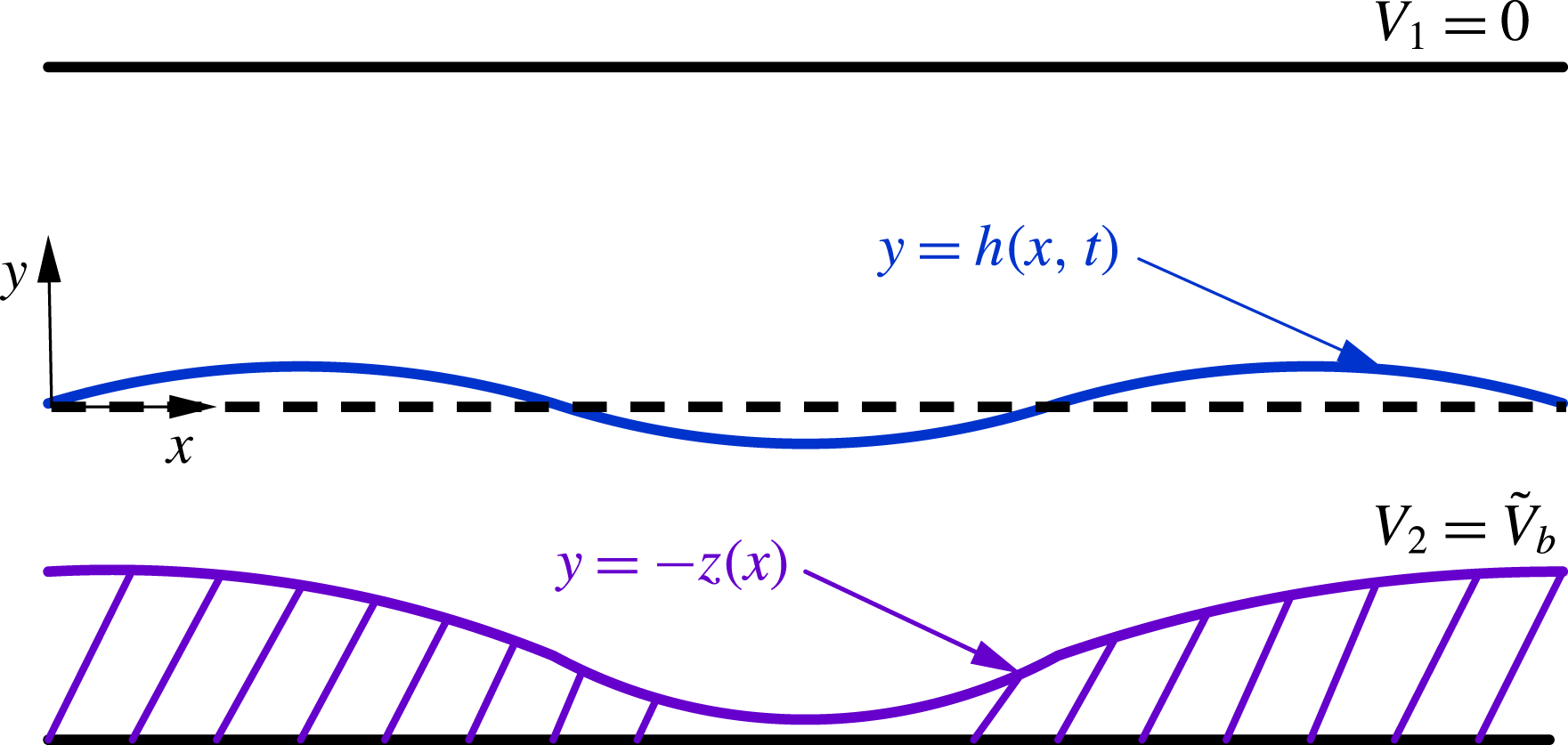
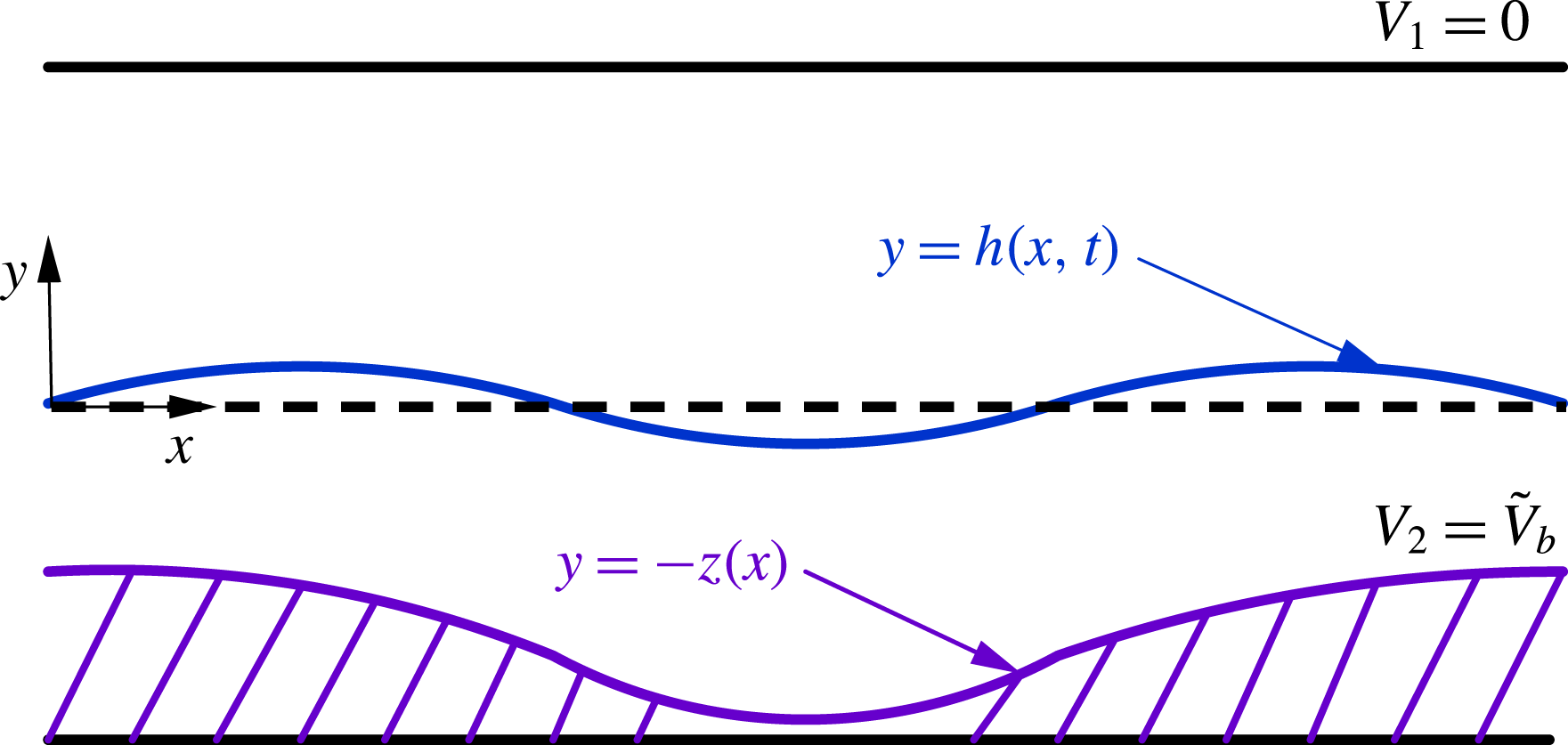
We consider the dynamics of two layers of immiscible viscous fluids that are placed between two electrodes; the top electrode is parallel to the undisturbed interface while the bottom electrode is patterned and its shape is given by
 $y=-z(x)$
(figure 1). The flow in the channel is driven by a pressure gradient and the overall flow rate through the channel is taken to be constant. The fluids are assumed to be perfect dielectrics and occupy the regions
 $h(x,t)\leqslant y\leqslant \unicode[STIX]{x1D6FD}H$
(fluid 1) and
 $-z(x)H\leqslant y\leqslant h(x,t)$
(fluid 2), where
 $y=h(x,t)$
denotes the interface location. The electrodes are kept at constant voltage potentials,
 $V_{1}=0$
at the top and
 $V_{2}=\tilde{V}_{b}$
at the bottom. In addition, the interfacial tension is constant and equal to
 $\unicode[STIX]{x1D6FE}$
.
Schematic of the problem studied. The lower boundary is structured topographically with a given position
 $y=-z(x)$
and is held at constant voltage
 $V_{2}=\tilde{V}_{b}$
. The upper wall is at
 $y=\unicode[STIX]{x1D6FD}H$
and is held at zero potential.
The fluids are taken to be Newtonian and incompressible, and the electric fields are governed by the electrostatic approximation of Maxwell’s equations. Here we give the general governing equations for the two fluids, assumed to be perfect dielectrics, and denoted as fluid 1 (upper) and fluid 2 (lower), and having viscosities
 $\unicode[STIX]{x1D707}_{1,2}$
, densities
 $\unicode[STIX]{x1D70C}_{1,2}$
and dielectric constants
 $\unicode[STIX]{x1D716}_{1,2}$
, respectively. The velocity in fluid
 $i$
(for
 $i=1,2$
) is
 $\boldsymbol{u}_{i}=(u_{i},v_{i},0)$
, where
 $u_{i}$
and
 $v_{i}$
are the components in the
 $x$
and
 $y$
directions, respectively;
 $P_{i}$
is the pressure in fluid
 $i$
. Owing to the small scale of the systems of interest here, gravity can be neglected.
The fluid flow is governed by the Navier–Stokes and continuity equations in each region
 $i=1,2$
:
 $$\begin{eqnarray}\displaystyle & \displaystyle \unicode[STIX]{x1D70C}_{i}(\boldsymbol{u}_{it}+\boldsymbol{u}_{i}\boldsymbol{\cdot }\unicode[STIX]{x1D735}\boldsymbol{u}_{i})=-\unicode[STIX]{x1D735}P_{i}+\unicode[STIX]{x1D707}_{i}\unicode[STIX]{x1D6FB}^{2}\boldsymbol{u}_{i}, & \displaystyle\end{eqnarray}$$
 $$\begin{eqnarray}\displaystyle & \displaystyle \unicode[STIX]{x1D735}\boldsymbol{\cdot }\boldsymbol{u}_{i}=0. & \displaystyle\end{eqnarray}$$
The above equations are solved together with interfacial boundary conditions that correspond to continuity of the fluid velocity at the interface and jumps in the normal and tangential stresses:
 $$\begin{eqnarray}\displaystyle [\boldsymbol{u}\boldsymbol{\cdot }\boldsymbol{n}]_{2}^{1}=[\boldsymbol{u}\boldsymbol{\cdot }\boldsymbol{t}]_{2}^{1}=0,\quad [\boldsymbol{n}\boldsymbol{\cdot }\unicode[STIX]{x1D64F}\boldsymbol{\cdot }\boldsymbol{n}]_{2}^{1}=\unicode[STIX]{x1D6FE}\unicode[STIX]{x1D705},\quad [\boldsymbol{t}\boldsymbol{\cdot }\unicode[STIX]{x1D64F}^{\boldsymbol{F}}\boldsymbol{\cdot }\boldsymbol{n}]_{2}^{1}=0. & & \displaystyle\end{eqnarray}$$
Here
 $[(\cdot )]_{2}^{1}$
denotes the jump in
 $(\cdot )$
as the interface is crossed from above;
 $\boldsymbol{n}=(-h_{x},1)/\sqrt{1+h_{x}^{2}}$
is the outward-pointing normal vector;
 $\boldsymbol{t}=(1,h_{x})/\sqrt{1+h_{x}^{2}}$
is the tangent vector; and
 $\unicode[STIX]{x1D705}=h_{xx}/(1+h_{x}^{2})^{3/2}$
is the mean curvature. The total stress tensor
 $\unicode[STIX]{x1D64F}=\unicode[STIX]{x1D64F}^{\boldsymbol{F}}+\unicode[STIX]{x1D64F}^{\boldsymbol{E}}$
has both a fluid part and an electrical part, given by
 $$\begin{eqnarray}\displaystyle \unicode[STIX]{x1D64F}^{\boldsymbol{F}}=-p\unicode[STIX]{x1D644}+\unicode[STIX]{x1D707}(\unicode[STIX]{x1D735}\boldsymbol{u}+\unicode[STIX]{x1D735}\boldsymbol{u}^{\text{T}}),\quad \unicode[STIX]{x1D64F}^{\boldsymbol{E}}=\unicode[STIX]{x1D716}_{i}(\boldsymbol{E}\boldsymbol{E}-{\textstyle \frac{1}{2}}|\boldsymbol{E}|^{2}\unicode[STIX]{x1D644}). & & \displaystyle\end{eqnarray}$$
Note that the Maxwell stress contribution drops out of the tangential stress balance in (2.3) after use of Gauss’s law, given below in (2.6a,b
). In addition, we have no slip and no penetration at both boundaries,
 $y=-z(x)H$
and
 $y=\unicode[STIX]{x1D6FD}H$
.
The electric field
 $\boldsymbol{E}_{i}$
is irrotational, hence it can be expressed by
 $\boldsymbol{E}_{i}=-\unicode[STIX]{x1D735}V_{i}$
, where the voltage potentials
 $V_{i}$
are governed by the Laplace equations
 $$\begin{eqnarray}\displaystyle \unicode[STIX]{x1D6FB}^{2}V_{i}=0. & & \displaystyle\end{eqnarray}$$
The boundary conditions across the interface are those of continuity of
 $V$
and continuity of the displacement field in the normal direction (the latter is Gauss’s law),
 $$\begin{eqnarray}\displaystyle V_{1}=V_{2},\quad [\unicode[STIX]{x1D716}\boldsymbol{E}\boldsymbol{\cdot }\boldsymbol{n}]_{2}^{1}=0\quad \text{on}~y=h(x,t). & & \displaystyle\end{eqnarray}$$
At the walls, the voltages are kept constant according to
 $$\begin{eqnarray}\displaystyle V_{1}=0\quad \text{at}~y=\unicode[STIX]{x1D6FD}H,\quad V_{2}=\tilde{V}_{b}\quad \text{at}~y=-z(x)H. & & \displaystyle\end{eqnarray}$$
To complete the system, we need a kinematic condition at the interface,
 $$\begin{eqnarray}\displaystyle v_{i}=h_{t}+u_{i}h_{x}\quad \text{on}~y=h(x,t), & & \displaystyle\end{eqnarray}$$
and an overall flow-rate condition that is prescribed (the resulting horizontal pressure gradient comes as part of the solution),
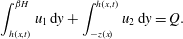 $$\begin{eqnarray}\displaystyle \int _{h(x,t)}^{\unicode[STIX]{x1D6FD}H}u_{1}\,\text{d}y+\int _{-z(x)}^{h(x,t)}u_{2}\,\text{d}y=Q. & & \displaystyle\end{eqnarray}$$
This set of nonlinear equations plus boundary conditions are a formidable nonlinear system, and to make progress we will utilise asymptotic methods to derive reduced-dimension nonlinear evolution equations that are valid for thin films.
2.2 Dimensionless equations
The equations are non-dimensionalised using the following scales:
 $$\begin{eqnarray}(x,y)=H(x^{\prime },y^{\prime }),\quad (u,v)=U(u^{\prime },v^{\prime }),\quad t=\frac{H}{U}t^{\prime },\quad V=V_{b}V^{\prime },\quad P=\frac{\unicode[STIX]{x1D707}_{1}U}{H}P^{\prime }.\end{eqnarray}$$
Here
 $U$
is a typical velocity scale, for example the velocity at the undisturbed interface of the equivalent straight-walled channel, and the scale
 $V_{b}$
will be chosen later in order to normalise to unity the coefficient of the electrical Maxwell stresses in the normal stress balance (2.12) below. The following non-dimensional equations emerge, where for simplicity all primes are dropped:
 $$\begin{eqnarray}\displaystyle & \displaystyle \mathit{Re}(u_{it}+u_{i}u_{ix}+v_{i}u_{iy})=-P_{ix}+m_{i}(u_{ixx}+u_{iyy}), & \displaystyle\end{eqnarray}$$
 $$\begin{eqnarray}\displaystyle & \displaystyle \mathit{Re}(v_{it}+u_{i}v_{ix}+v_{i}v_{iy})=-P_{iy}+m_{i}(v_{ixx}+v_{iyy}), & \displaystyle\end{eqnarray}$$
 $$\begin{eqnarray}\displaystyle & \displaystyle u_{ix}+v_{iv}=0, & \displaystyle\end{eqnarray}$$
 $$\begin{eqnarray}\displaystyle & \displaystyle V_{ixx}+V_{iyy}=0. & \displaystyle\end{eqnarray}$$
The dimensionless normal and tangential stress balances (see (2.3)) become, at
 $y=h(x,t)$
,
 $$\begin{eqnarray}\displaystyle & & \displaystyle \left[-P_{i}+\frac{2}{1+h_{x}^{2}}\left[m_{i}v_{iy}(1-h_{x}^{2})-m_{i}h_{x}(u_{iy}+v_{ix})\right]\right.\nonumber\\ \displaystyle & & \displaystyle \quad \left.+\,\bar{\unicode[STIX]{x1D716}}_{i}\frac{1-h_{x}^{2}}{2(1+h_{x}^{2})}(V_{iy}^{2}-V_{ix}^{2})-\frac{2\bar{\unicode[STIX]{x1D716}}_{i}h_{x}}{1+h_{x}^{2}}V_{ix}V_{iy}\right]_{2}^{1}=\frac{h_{xx}}{Ca(1+h_{x}^{2})^{3/2}},\end{eqnarray}$$
 $$\begin{eqnarray}\displaystyle & & \displaystyle \left[4h_{x}m_{i}v_{iy}+(1-h_{x}^{2})(m_{i}u_{iy}+m_{i}v_{ix})\right]_{2}^{1}=0,\end{eqnarray}$$
while the continuity of velocity at the interface, the kinematic condition and the overall flow-rate condition (see (2.9)) transform to
 $$\begin{eqnarray}\displaystyle u_{1}=u_{2},\quad v_{1}=v_{2}\quad \text{on}~y=h(x,t), & & \displaystyle\end{eqnarray}$$
 $$\begin{eqnarray}\displaystyle & \displaystyle v_{1,2}=h_{t}+u_{1,2}h_{x}\quad \text{on}~y=h(x,t), & \displaystyle\end{eqnarray}$$
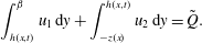 $$\begin{eqnarray}\displaystyle & \displaystyle \int _{h(x,t)}^{\unicode[STIX]{x1D6FD}}u_{1}\,\text{d}y+\int _{-z(x)}^{h(x,t)}u_{2}\,\text{d}y=\tilde{Q}. & \displaystyle\end{eqnarray}$$
The voltage continuity and Gauss’s law conditions (2.6) become, at
 $y=h(x,t)$
,
 $$\begin{eqnarray}\displaystyle V_{1}=V_{1},\quad [\bar{\unicode[STIX]{x1D716}}_{i}(h_{x}\,V_{ix}-V_{iy})]_{2}^{1}=0. & & \displaystyle\end{eqnarray}$$
Finally, the boundary conditions for the velocity and voltage at the upper and lower walls become
 $$\begin{eqnarray}\displaystyle u_{1}=0,\quad V_{1}=0\quad \text{at}~y=\unicode[STIX]{x1D6FD}, & & \displaystyle\end{eqnarray}$$
 $$\begin{eqnarray}\displaystyle u_{2}=0,\quad V_{2}=V_{b}\quad \text{at}~y=-z(x). & & \displaystyle\end{eqnarray}$$
In the process of the non-dimensionalisation, the following dimensionless parameters emerge:
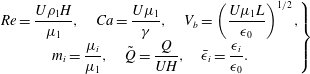 $$\begin{eqnarray}\displaystyle \left.\begin{array}{@{}c@{}}\displaystyle \mathit{Re}=\frac{U\unicode[STIX]{x1D70C}_{1}H}{\unicode[STIX]{x1D707}_{1}},\quad Ca=\frac{U\unicode[STIX]{x1D707}_{1}}{\unicode[STIX]{x1D6FE}},\quad V_{b}=\left(\frac{U\unicode[STIX]{x1D707}_{1}L}{\unicode[STIX]{x1D716}_{0}}\right)^{1/2},\\ \displaystyle m_{i}=\frac{\unicode[STIX]{x1D707}_{i}}{\unicode[STIX]{x1D707}_{1}},\quad \tilde{Q}=\frac{Q}{UH},\quad \bar{\unicode[STIX]{x1D716}}_{i}=\frac{\unicode[STIX]{x1D716}_{i}}{\unicode[STIX]{x1D716}_{0}}.\end{array}\right\} & & \displaystyle\end{eqnarray}$$
Here
 $\mathit{Re}$
is the Reynolds number,
 $Ca$
is the capillary number,
 $V_{b}$
is the dimensionless voltage imposed at the lower wall
 $y=-z(x)$
,
 $\tilde{Q}$
is the dimensionless flow rate,
 $m_{2}$
is the viscosity ratio of lower to upper fluid, and
 $\bar{\unicode[STIX]{x1D716}}_{i}$
are the relative electrical permittivities in each region with respect to that of free space
 $\unicode[STIX]{x1D716}_{0}$
. We also note that the problem is solved subject to periodic boundary conditions in
 $x$
when
 $z(x)$
is spatially periodic; in such cases the pressure gradient can be written as a constant plus a spatially periodic part of zero spatial mean.
2.3 Long-wave analysis and derivation of evolution equations
In the analysis that follows we assume that the wavelength
 $\unicode[STIX]{x1D706}$
of interfacial disturbances is long compared to the channel height
 $H$
and take
 $\unicode[STIX]{x1D6FF}=H/\unicode[STIX]{x1D706}\ll 1$
. We make the following change of variables in each region
 $i=1,2$
:
 $$\begin{eqnarray}\displaystyle u_{i}=\tilde{u} _{i},\quad v_{i}=\unicode[STIX]{x1D6FF}\tilde{v}_{i},\quad x=\frac{\hat{x}}{\unicode[STIX]{x1D6FF}},\quad t=\frac{\hat{t}}{\unicode[STIX]{x1D6FF}},\quad P_{i}=\frac{\tilde{P}_{i}}{\unicode[STIX]{x1D6FF}},\quad V_{i}=\tilde{V}_{i}. & & \displaystyle\end{eqnarray}$$
For convenience, the hats on the independent variables
 $\hat{x}$
and
 $\hat{t}$
are now dropped. The scaling for the vertical velocities
 $v_{i}$
comes from the continuity equations while the one for the pressures is needed for the flow to be driven by the pressure gradient at leading order (see e.g. Craster & Matar Reference Craster and Matar2009, and references therein). In order to retain electric field and surface tension effects, we are led to the canonical asymptotic limit of strong surface tension and high contrast permittivities in the two fluids, namely
 $Ca\sim \unicode[STIX]{x1D6FF}^{3}$
and
 $\bar{\unicode[STIX]{x1D716}}_{i}\sim 1/\unicode[STIX]{x1D6FF}$
. Note that other limits are possible, for example weaker surface tension and comparable electrical permittivities
 $Ca\sim \unicode[STIX]{x1D6FF}^{2}$
and
 $\bar{\unicode[STIX]{x1D716}}_{i}\sim 1$
, which can yield Benney-type equations with small regularising terms containing inertia – see Tseluiko & Papageorgiou (Reference Tseluiko and Papageorgiou2006) for electrified falling films on flat substrates. In addition we take the Reynolds number to be small,
 $\mathit{Re}\sim \unicode[STIX]{x1D6FF}$
, since we are interested in small-scale geometries with applications in microfluidics. The solutions are expanded in powers of
 $\unicode[STIX]{x1D6FF}$
as
 $$\begin{eqnarray}(\tilde{u} _{i},\tilde{v}_{i},\tilde{P}_{i},\tilde{V}_{i})=(u_{i}^{(0)},v_{i}^{(0)},p_{i}^{(0)},V_{i}^{(0)})+\unicode[STIX]{x1D6FF}(u_{i}^{(1)},v_{i}^{(1)},p_{i}^{(1)},V_{i}^{(1)})+O(\unicode[STIX]{x1D6FF}^{2}),\end{eqnarray}$$
and at leading order the system (2.8)–(2.11) yields
 $$\begin{eqnarray}\displaystyle m_{i}u_{iyy}^{(0)}=p_{ix}^{(0)},\quad p_{iy}^{(0)}=0,\quad u_{ix}^{(0)}+v_{iy}^{(0)}=0,\quad V_{iyy}^{(0)}=0. & & \displaystyle\end{eqnarray}$$
The interfacial conditions (2.12)–(2.18) and (2.20) become, at leading order,
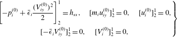 $$\begin{eqnarray}\displaystyle \left.\begin{array}{@{}c@{}}\displaystyle \left[-p_{i}^{(0)}+\bar{\unicode[STIX]{x1D716}}_{i}\frac{(V_{iy}^{(0)})^{2}}{2}\right]_{2}^{1}=h_{xx},\quad [m_{i}u_{iy}^{(0)}]_{2}^{1}=0,\quad [u_{i}^{(0)}]_{2}^{1}=0,\\ \displaystyle [-\bar{\unicode[STIX]{x1D716}}_{i}V_{iy}^{(0)}]_{2}^{1}=0,\quad [V_{i}^{(0)}]_{2}^{1}=0,\end{array}\right\} & & \displaystyle\end{eqnarray}$$
while the overall flow-rate condition (2.19) gives
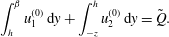 $$\begin{eqnarray}\displaystyle \int _{h}^{\unicode[STIX]{x1D6FD}}u_{1}^{(0)}\,\text{d}y+\int _{-z}^{h}u_{2}^{(0)}\,\text{d}y=\tilde{Q}. & & \displaystyle\end{eqnarray}$$
Solving (2.26) along with the interfacial conditions (2.27) and the boundary conditions (2.21) and (2.22) gives the following expressions for the horizontal velocities and the voltages:
 $$\begin{eqnarray}\displaystyle u_{1}^{(0)}=\frac{p_{1x}^{(0)}}{2m_{1}}(y^{2}-\unicode[STIX]{x1D6FD}^{2})+f_{1}(x,t)(y-\unicode[STIX]{x1D6FD}),\quad u_{2}^{(0)}=\frac{p_{2x}^{(0)}}{2m_{2}}(y^{2}-z^{2})+f_{2}(x,t)(y+z), & & \displaystyle \nonumber\\ \displaystyle & & \displaystyle\end{eqnarray}$$
 $$\begin{eqnarray}\displaystyle V_{1}^{(0)}=d_{1}(x,t)(y-\unicode[STIX]{x1D6FD}),\quad V_{2}^{(0)}=d_{2}(x,t)(y+z)+V_{b}. & & \displaystyle\end{eqnarray}$$
Here
 $d_{i}(x,t)$
,
 $f_{i}(x,t)$
and
 $p_{ix}^{(0)}(x,t)$
for
 $i=1,2$
are functions of
 $h(x,t)$
and its derivatives – see appendix A for details. Finally, the kinematic condition is written in integral form using the continuity equation (2.11) as in Papaefthymiou, Papageorgiou & Pavliotis (Reference Papaefthymiou, Papageorgiou and Pavliotis2013) for example:
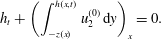 $$\begin{eqnarray}\displaystyle h_{t}+\left(\int _{-z(x)}^{h(x,t)}u_{2}^{(0)}\,\text{d}y\right)_{x}=0. & & \displaystyle\end{eqnarray}$$
Substituting the leading-order solutions (2.29) and (2.30) found above into (2.31) leads to the following evolution equation for the interfacial position
 $h(x,t)$
:
 $$\begin{eqnarray}\displaystyle h_{t}+\left\{\frac{D_{3}}{6m_{2}}\left[D_{4}p_{2x}^{(0)}+3m_{2}f_{2}\right]\right\}_{x}=0, & & \displaystyle\end{eqnarray}$$
where
 $D_{3}=(h(x,t)+z(x))^{2}$
and
 $D_{4}=h(x,t)-2z(x)$
(see appendix A for details of the functions involved). It should be stressed that, once the interfacial amplitude
 $h(x,t)$
is determined, then the leading-order flow and voltage potential throughout the channel follow from the solutions (2.29) and (2.30). Such expressions are used in the sequel when constructing instantaneous (or steady-state) streamlines to visualise the flow and obtain information about the distribution of vorticity in the microchannel.
Equation (2.32) is solved numerically using spectral methods in space and the stiff ordinary differential equation (ODE) solver DASSL in time (see Petzold Reference Petzold and Stepleman1983). The latter is a Fortran package that approximates derivatives using backward differentiation formulae of order
 $p$
with
 $1\leqslant p\leqslant 5$
; the order
 $p$
and the time step size are selected adaptively in order to keep errors below a desired tolerance level. The discretisation results in a large nonlinear system that is solved efficiently and accurately using a Newton’s method. The initial condition used in our computations is
 $$\begin{eqnarray}h(x,0)=h_{0}\cos (kx),\end{eqnarray}$$
with
 $h_{0}=0.01$
(or
 $h_{0}=0$
when stated) and different values of the wavenumber
 $k$
. The initial condition (2.33) is
 $2\unicode[STIX]{x03C0}/k$
periodic and typically the evolution equation (2.32) is also solved on a periodic domain of length
 $2\unicode[STIX]{x03C0}/k$
. We have also carried out computations on longer domains that are integer multiples of
 $2\unicode[STIX]{x03C0}/k$
, in order to investigate the possibility of subharmonic instabilities. The numerical integration is carried out to large enough times to enable identification of the types of solutions that emerge.
2.4 Linear stability for flat boundaries
When the lower boundary is wavy, the base state is non-uniform and its stability is not amenable to a normal-mode analysis – Floquet theory is used instead, as detailed later in § 5. To gain an understanding of the underlying instabilities present, in what follows we perform a linear stability analysis for a flat lower electrode placed at
 $y=-Z_{c}=0.9$
. Note that this analysis is a special case of that in Ozen et al. (Reference Ozen, Aubry, Papageorgiou and Petropoulos2006) and Li et al. (Reference Li, Ozen, Aubry, Papageorgiou and Petropoulos2007) – it is the inertialess long-wave version of those studies and we include it for completeness and guidance for the wavy-boundary nonlinear work that follows. In this case the evolution equation is linearised about the steady state
 $h\equiv 0$
and solutions proportional to
 $\exp (\text{i}kx+st)$
are sought, leading to a dispersion relation for the growth rate
 $s$
as a function of the wavenumber
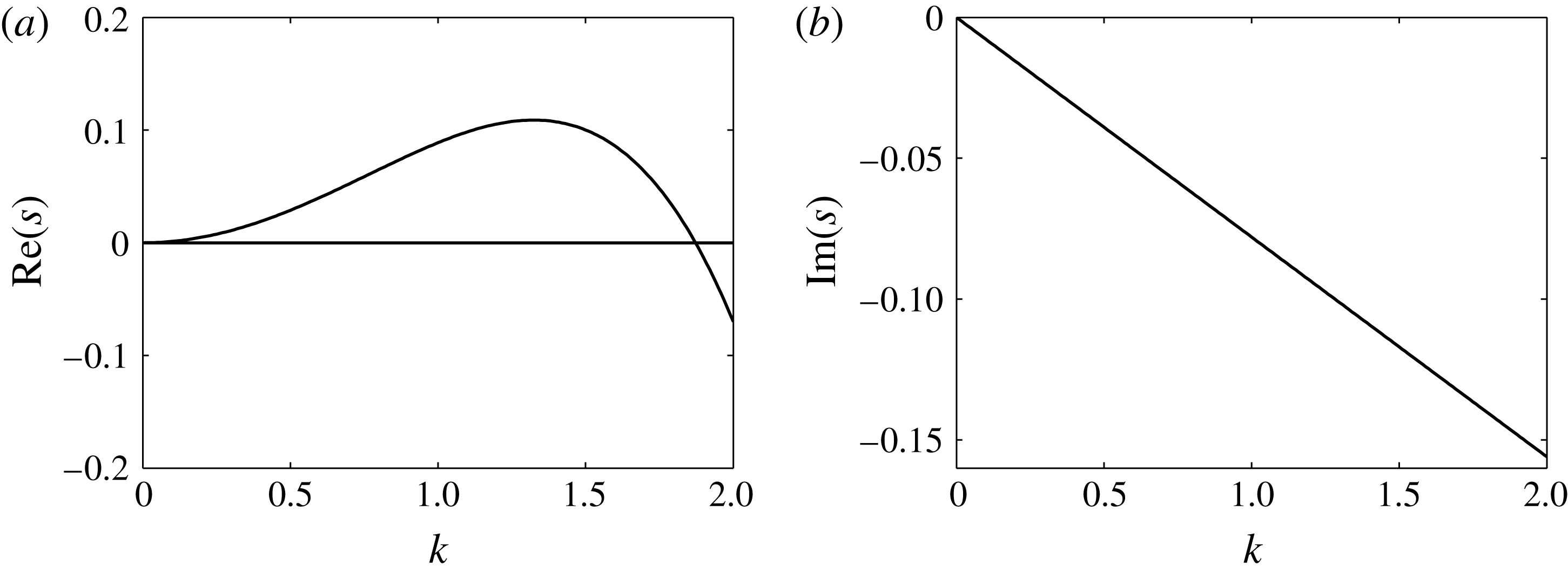
 $k$
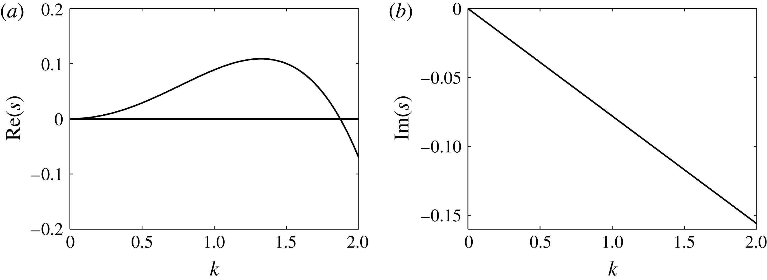
. Figure 2(a) shows the real part of
 $s$
, which is the growth rate, and figure 2(b) shows its imaginary part, which is the frequency. This is done for a typical set of physical parameters with an imposed dimensionless voltage
 $V_{b}=3$
, a flow rate
 $\tilde{Q}=0.1$
, a unit channel height described by
 $\unicode[STIX]{x1D6FD}=1$
, relative permittivities
 $\bar{\unicode[STIX]{x1D716}}_{1}=1$
and
 $\bar{\unicode[STIX]{x1D716}}_{2}=5$
, and equal viscosities so that
 $m_{1}=m_{2}=1$
. In order to reduce the large set of parameters that characterise our problem, we proceed with equal viscosities throughout the rest of the paper. The results show that the flow is long-wave unstable with a finite band of unstable modes with short waves (large
 $k$
) damped. In addition, the imaginary part of
 $s$
is non-zero and in fact linear in
 $k$
, hence linear waves are predicted to travel with a constant phase velocity. Hence we can expect that, after nonlinear saturation, the emerging structures will tend to travel in the direction of increasing
 $x$
. The precise nature of the emerging coherent structures is undertaken next through detailed numerical computations.
Linear growth rate for flat bottom walls at
 $y=-0.9$
and for an applied dimensionless voltage
 $V_{b}=3$
. Other parameters are the dimensionless flow rate
 $\tilde{Q}=0.1$
,
 $\unicode[STIX]{x1D6FD}=1$
(i.e. the upper wall is at
 $y=1$
), dimensionless permittivities
 $\bar{\unicode[STIX]{x1D716}}_{1}=1$
and
 $\bar{\unicode[STIX]{x1D716}}_{2}=5$
, and viscosity ratio
 $m_{2}=1$
.
3 Flat lower boundary: formation of directed assembly travelling wave structures
We begin our numerical studies by considering the case when the lower electrode is flat and placed at
 $y=-Z_{c}$
, where
 $Z_{c}>0$
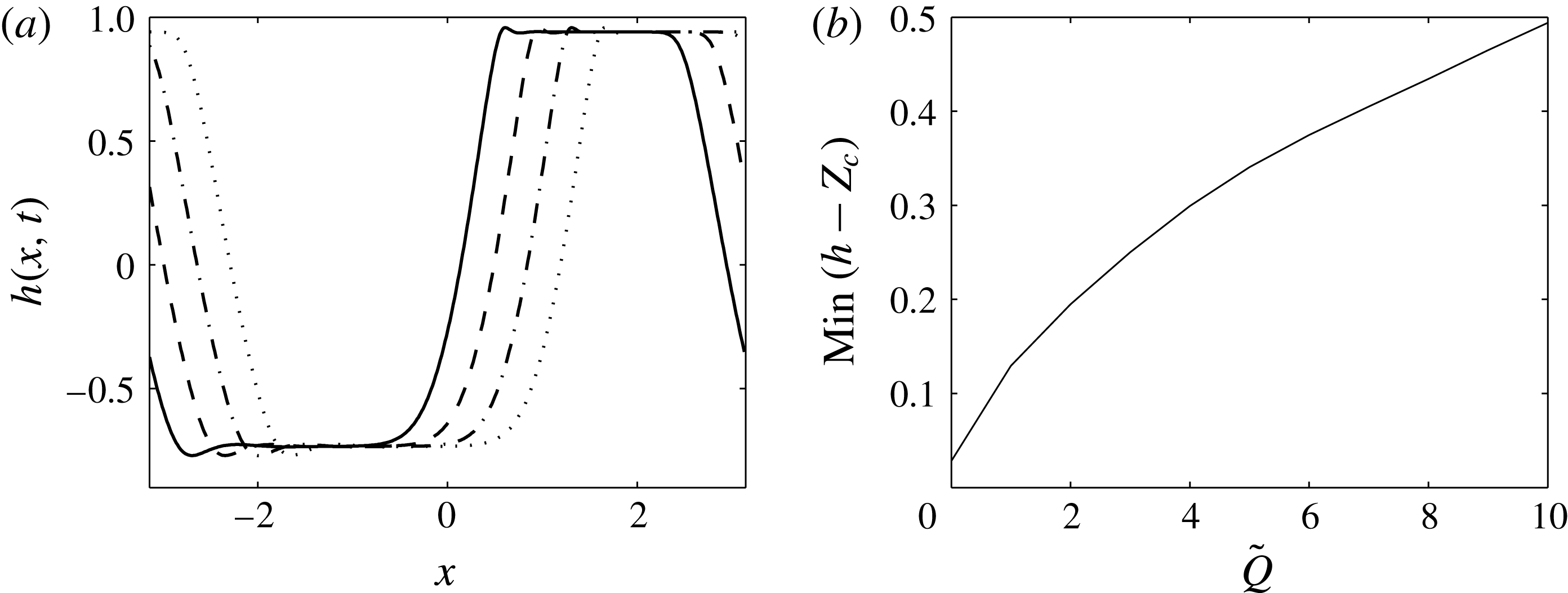
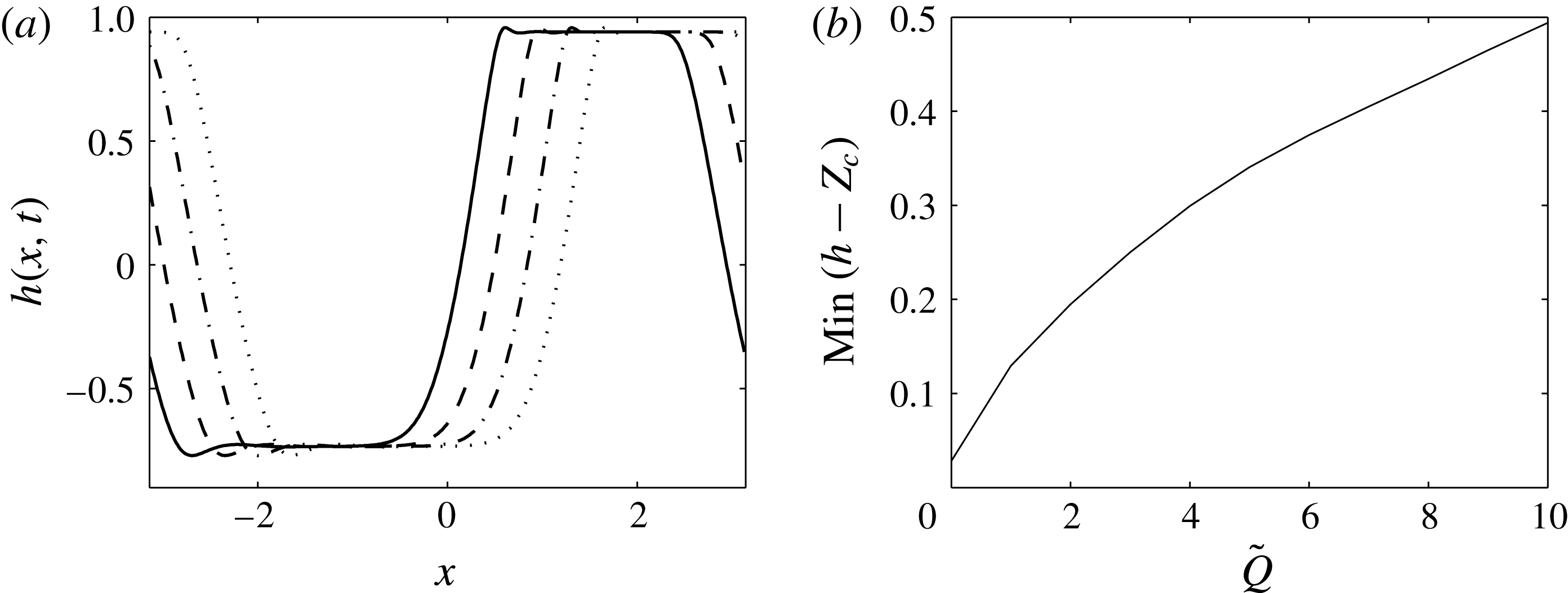
is a constant. Figure 3(a) shows the interfacial deformation
 $h(x,t)$
at four consecutive relatively large times, ensuring transients have died out; here
 $Z_{c}=0.9$
so that the dimensionless channel thickness is 1.9 units, and the other parameters are as in figure 2 so that the
 $k=1$
mode is unstable. The solid curve corresponds to
 $t=200$
, the dashed curve to
 $t=200.6$
, the dot-dashed curve to
 $t=201.2$
, and the dotted curve to
 $t=201.8$
. The linear instabilities saturate to what appear to be nonlinear travelling waves that span almost the whole extent of the channel. The interface approaches the boundaries but remains at a small but finite distance from them for the whole duration of the computation – such behaviour has been confirmed for much longer computations with times as large as
 $10^{4}$
and different parameters. This is in contrast to situations with no background flow, i.e.
 $\tilde{Q}=0$
in our notation, where electrostatic instabilities lead to interfacial contact with the wall – see for example the theoretical studies of Craster & Matar (Reference Craster and Matar2005), Tseluiko & Papageorgiou (Reference Tseluiko and Papageorgiou2007a
,Reference Tseluiko and Papageorgiou
b
) and Barannyk et al. (Reference Barannyk, Papageorgiou, Petropoulos and Vanden-Broeck2015) for both planar and cylindrical geometries as well as fields acting parallel to the undisturbed interface, as well as the experiments of Schaffer et al. (Reference Schaffer, Thurn-Albrecht, Russell and Steiner2001). In figure 3(b) we quantify these observations in the presence of flow by monitoring the minimum distance of the interface to the walls as
 $\tilde{Q}$
varies – to fix matters we do this for different runs and calculate minimal approaches at a large time
 $t=300$
. The results indicate that the minimum distance increases as
 $\tilde{Q}$
increases, thus confirming the earlier findings that there is a flow-induced stabilisation of touchdown events. As mentioned already, when
 $\tilde{Q}=0$
, we expect asymptotic thinning with touchdown as
 $t\rightarrow \infty$
, and the finite value of approximately
 $0.02$
given in figure 3(b) reflects the fact that
 $t$
is not large enough – larger
 $t$
would lead to smaller values (see e.g. Craster & Matar Reference Craster and Matar2005; Tseluiko & Papageorgiou Reference Tseluiko and Papageorgiou2007b
). Similar stabilising effects due to flow are found, for instance, when van der Waals forces are present that would otherwise cause film rupture (Bielarz & Kalliadasis Reference Bielarz and Kalliadasis2003; Kalpathy, Francis & Kumar Reference Kalpathy, Francis and Kumar2010; Davis, Gratton & Davis Reference Davis, Gratton and Davis2010).
(a) Interface
 $h(x,t)$
at
 $t=200$
(solid curve),
 $t=200.6$
(dashed curve),
 $t=201.2$
(dot-dashed curve) and
 $t=201.8$
(dotted curve). Walls are at
 $y=-0.9$
(
 $Z_{c}=0.9$
) and
 $y=1$
(
 $\unicode[STIX]{x1D6FD}=1$
). Other parameters are
 $\tilde{Q}=1$
,
 $V_{b}=3$
,
 $\bar{\unicode[STIX]{x1D716}}_{1}=1$
,
 $\bar{\unicode[STIX]{x1D716}}_{2}=5$
and
 $m_{2}=1$
. (b) Minimum distance between the interface and the lower boundary at time
 $t=300$
as the flow rate
 $\tilde{Q}$
varies.
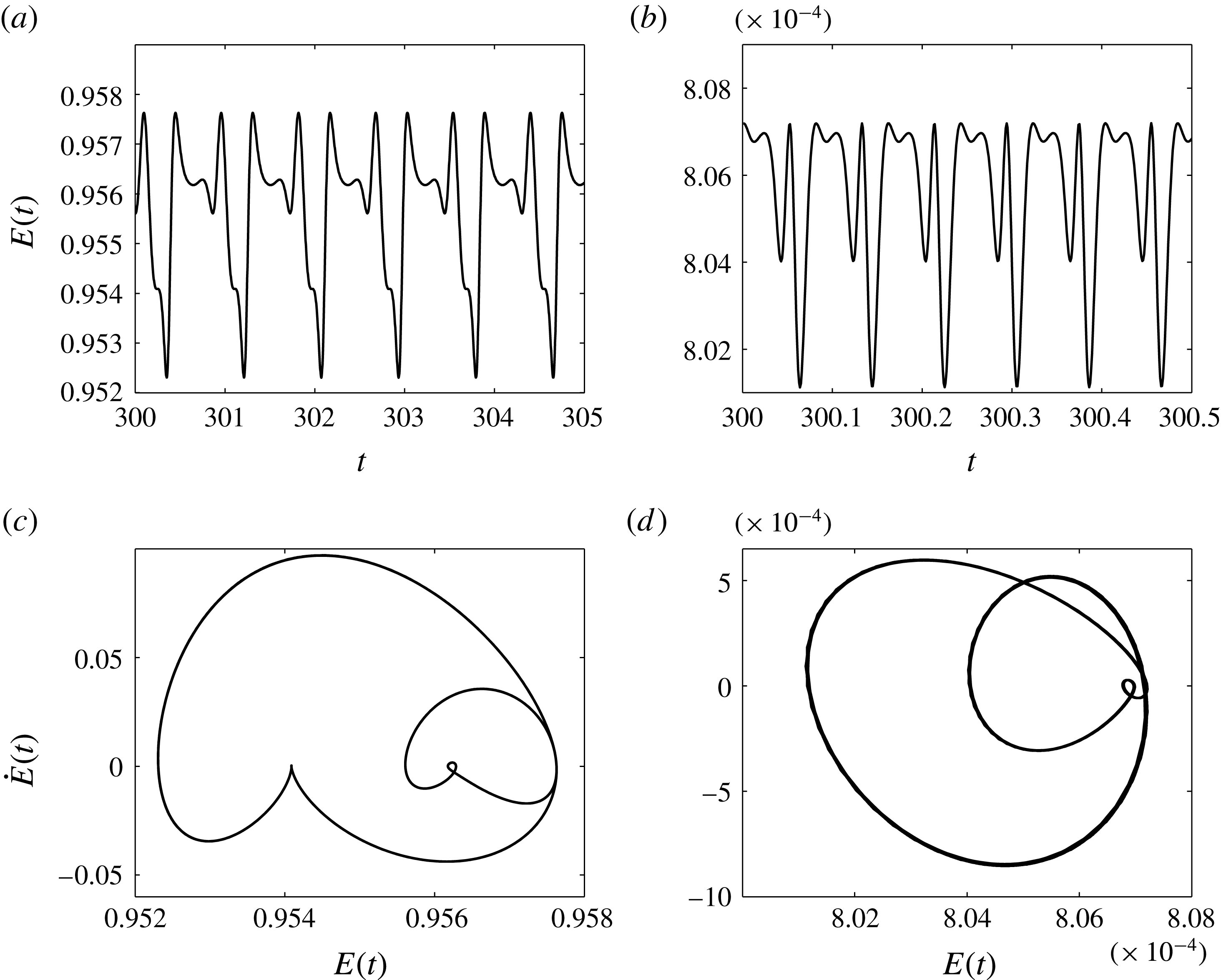
Even though the solutions presented in figure 3(a) appear to be nonlinear travelling waves, closer analysis of the data establishes that they are in fact travelling time-periodic waves – such structures have been found in simpler weakly nonlinear model equations such as the Kuramoto–Sivashinsky equation (see e.g. Akrivis, Papageorgiou & Smyrlis Reference Akrivis, Papageorgiou and Smyrlis2011). To accurately predict such dynamics we make use of the energy of the solution defined as
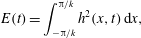 $$\begin{eqnarray}\displaystyle E(t)=\int _{-\unicode[STIX]{x03C0}/k}^{\unicode[STIX]{x03C0}/k}h^{2}(x,t)\,\text{d}x, & & \displaystyle\end{eqnarray}$$
and note that this is computed with spectral accuracy either using Parseval’s theorem, since the Fourier coefficients are known, or using trapezoidal quadrature, which is spectrally accurate for periodic functions; we also calculate
 $\text{d}E/\text{d}t$
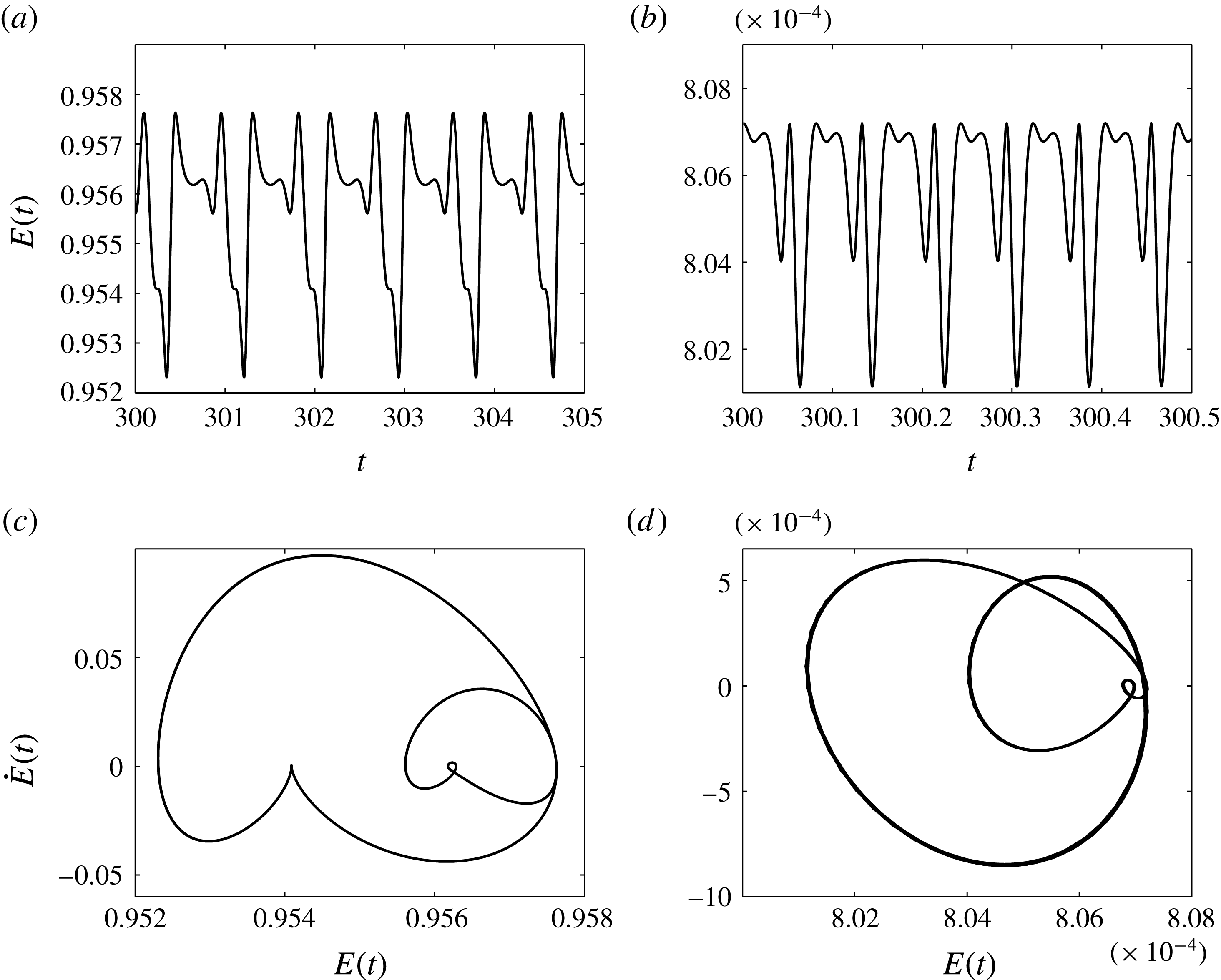
in order to construct the phase planes presented below. Figure 4(a,b) gives the evolution of
 $E(t)$
for
 $\tilde{Q}=10$
and
 $100$
, respectively. In both cases we observe time-periodic behaviour (approximately five periods of oscillation are included in each case) with the period decreasing as
 $\tilde{Q}$
increases. In fact the period for
 $\tilde{Q}=10$
is approximately equal to
 $0.8$
time units, while that for
 $\tilde{Q}=100$
it is approximately
 $0.08$
time units, a decrease by a factor of
 $10$
, indicating that the frequency of oscillation is proportional to
 $\tilde{Q}$
when this becomes large – an asymptotic theory along with comparisons with the numerical data is presented in § 6.1 for the more complicated case of wavy lower boundaries. Another feature of the results in figure 4(a,b) is the small amplitude of the time-dependent oscillations about a mean value, with these amplitudes again decreasing as
 $\tilde{Q}$
increases. Confirmation of the time periodicity of the solution is provided in the phase-plane plots in figure 4(c,d) that have been produced for longer time intervals than those shown in figure 4(a,b). The two distinct loops correspond to the small- and large-amplitude superimposed oscillations of the two time signals.
(a,b) Time evolution of the energy
 $E(t)$
for (a)
 $\tilde{Q}=10$
and (b)
 $\tilde{Q}=100$
. (c,d) Phase planes of the energy,
 $E$
versus
 $\text{d}E/\text{d}t$
, for (c)
 $\tilde{Q}=10$
and (d)
 $\tilde{Q}=100$
. All other parameters are the same as in figure 3.
We conclude that the dynamics in channels with flat walls leads to the formation of periodic ‘pillars’ similar to the ones found experimentally by Schaffer et al. (Reference Schaffer, Thurn-Albrecht, Russell and Steiner2001) and theoretically by Craster & Matar (Reference Craster and Matar2005) in the absence of a background flow. However, owing to the presence of flow, these structures travel down the channel and also undergo time-periodic modulations while keeping a finite separation distance from the walls.
4 Wavy lower boundary: interfacial response to non-uniform confinement geometries
In this section we present results of computations of (2.32) for a sinusoidal lower boundary given by
 $$\begin{eqnarray}y=-z(x)=-Z_{c}+d_{b}\cos (k_{b}\,x).\end{eqnarray}$$
The initial condition is (2.33) as before – recall that
 $2\unicode[STIX]{x03C0}/k$
selects the length of the computational domain. The parameter
 $d_{b}$
measures the wall amplitude and
 $k_{b}$
its wavenumber. When
 $d_{b}=0$
we reduce to the flat case and we will use the linear stability results of § 2.4 to guide the computations when
 $d_{b}\neq 0$
. In particular, for a given set of parameters, the linear theory predicts a critical wavenumber
 $k_{c}$
below which instability is supported, and we investigate the two cases (a)
 $k<k_{c}$
and (b)
 $k>k_{c}$
to show that they delineate distinct types of large-time solutions. In case (b) the interface very quickly reaches a steady state and adopts the wavenumber
 $k_{b}$
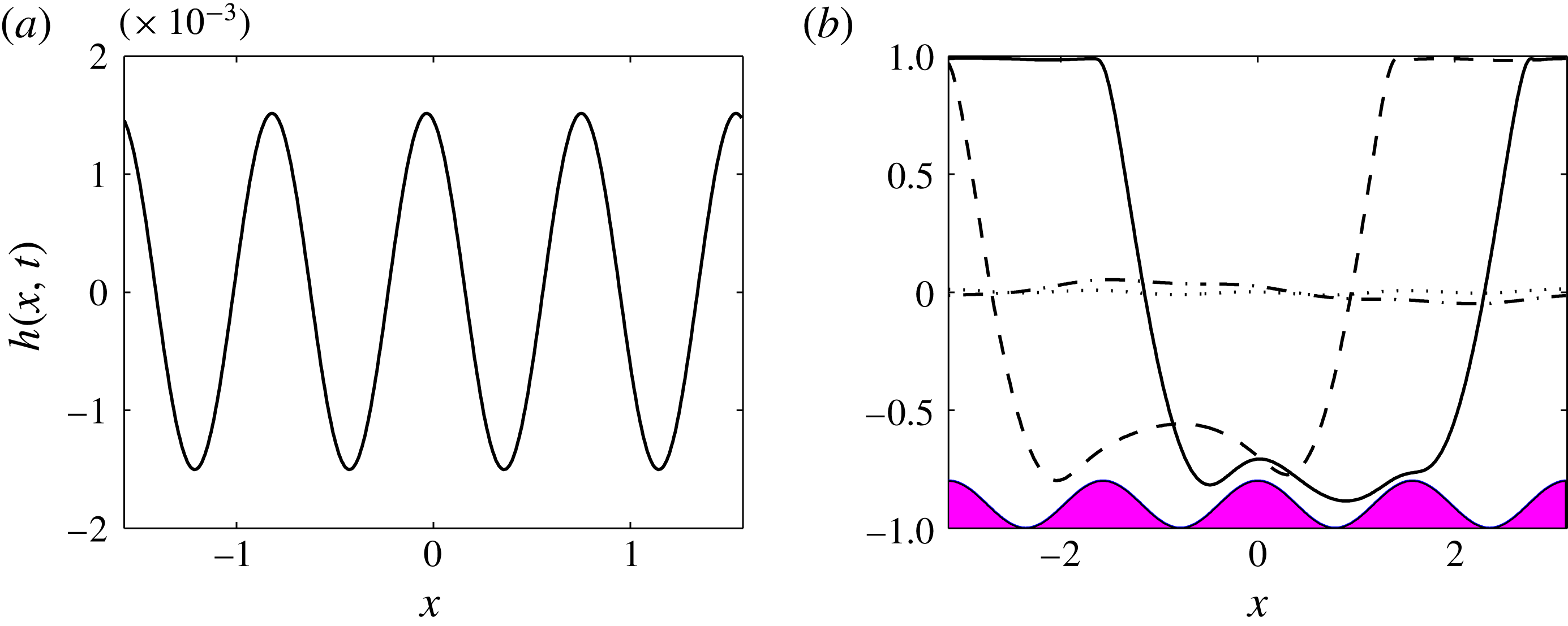
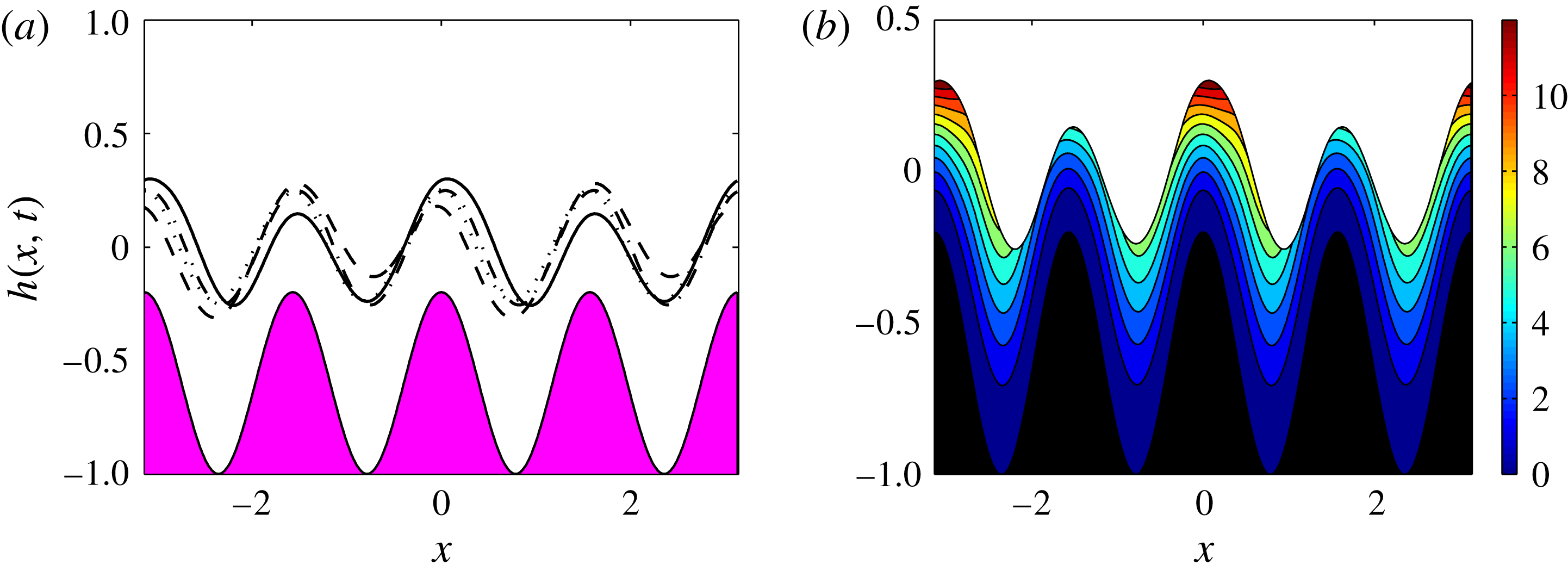
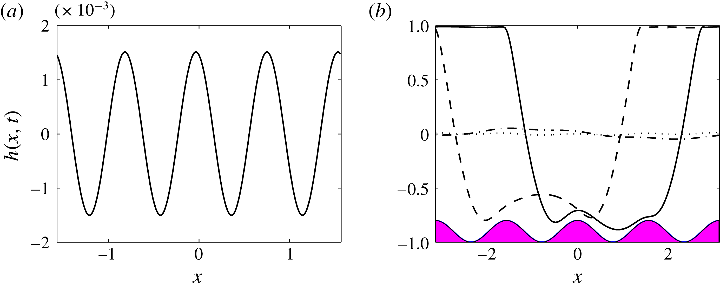
of the wavy boundary but with a much smaller amplitude; in case (a) we find travelling time-periodic structures that are similar to those for the flat-boundary case seen in figure 3, but are modulated due to the wavy confining wall and ‘squeeze’ past it. Typical results are given in figure 5 for wall parameters
 $k_{b}=4$
and
 $d_{b}=0.1$
and mean position
 $y=-Z_{c}=-0.9$
; the other parameters are
 $\tilde{Q}=0.1$
and
 $V_{b}=3$
. The results in figure 5(a) correspond to an initial condition having
 $k=2$
, i.e. it is twice the wavelength of the wavy wall. Note that this is larger than
 $k_{c}$
for the chosen parameters and so the flow reaches a steady state (
 $h$
is shown at
 $t=100$
here) with the interface inheriting the pattern of the wavy wall but with a smaller amplitude of roughly
 $1.5\times 10^{-3}$
compared with
 $d_{b}=0.1$
. In figure 5(b) we set
 $k=1<k_{c}$
and observe that the unstable longer-wavelength perturbation grows nonlinearly to travelling pillar-like structures found for flat walls, but at the same time sweeps over the topography, modulating its shape as it moves downstream. Profiles are shown at times ranging from
 $t=1$
(dotted curve) to
 $t=100$
(solid curve) and, as found previously for flat walls, throughout the evolution the interface gets close to the upper and lower walls but does not touch them.
Flow past a sinusoidal wavy wall of mean position
 $y=-0.9$
and having amplitude
 $d_{b}=0.1$
and wavenumber
 $k_{b}=4$
and
 $k_{c}=1.87$
; the scaled relative permittivities are
 $\bar{\unicode[STIX]{x1D716}}_{1}=1$
and
 $\bar{\unicode[STIX]{x1D716}}_{2}=5$
, the flow rate is
 $\tilde{Q}=0.1$
and the lower wall potential is
 $V_{b}=3$
. (a) Initial condition (2.33) with
 $k=2$
. Interface
 $h(x,t)$
is shown at time
 $t=100$
after the solution has reached steady state. (b) Longer initial perturbation having
 $k=1$
. Interface
 $h(x,t)$
at
 $t=1$
(dotted line),
 $t=25$
(dot-dashed line),
 $t=75$
(dashed line) and
 $t=100$
(solid line). The shaded area represents the lower boundary. A movie of the simulation for case (b) (movie 1) can be found in the supplementary material available at https://doi.org/10.1017/jfm.2017.17.
The results presented in figure 5 can be understood with a more detailed comparison with linear theory for flat walls. We can anticipate that, as long as the wall amplitude
 $d_{b}$
is not large – in the results
 $d_{b}=0.1$
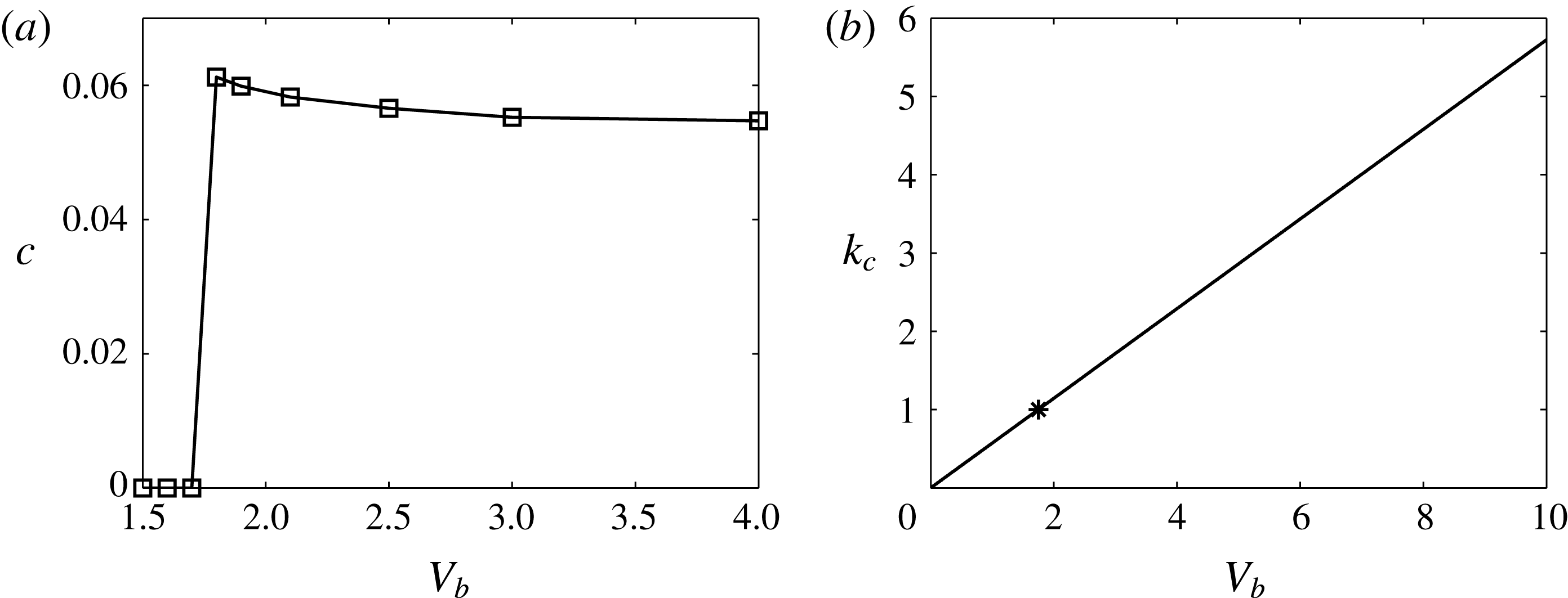
– the bifurcation from a non-uniform steady state to a more complicated modulated travelling wave should correlate with flat-wall linear theory. This is confirmed in the results presented in figure 6. We fix
 $k=1$
in the initial conditions and compute solutions for a wavy wall having
 $d_{b}=0.1$
and
 $k_{b}=1$
at increasing values of
 $V_{b}$
starting from
 $V_{b}=1.5$
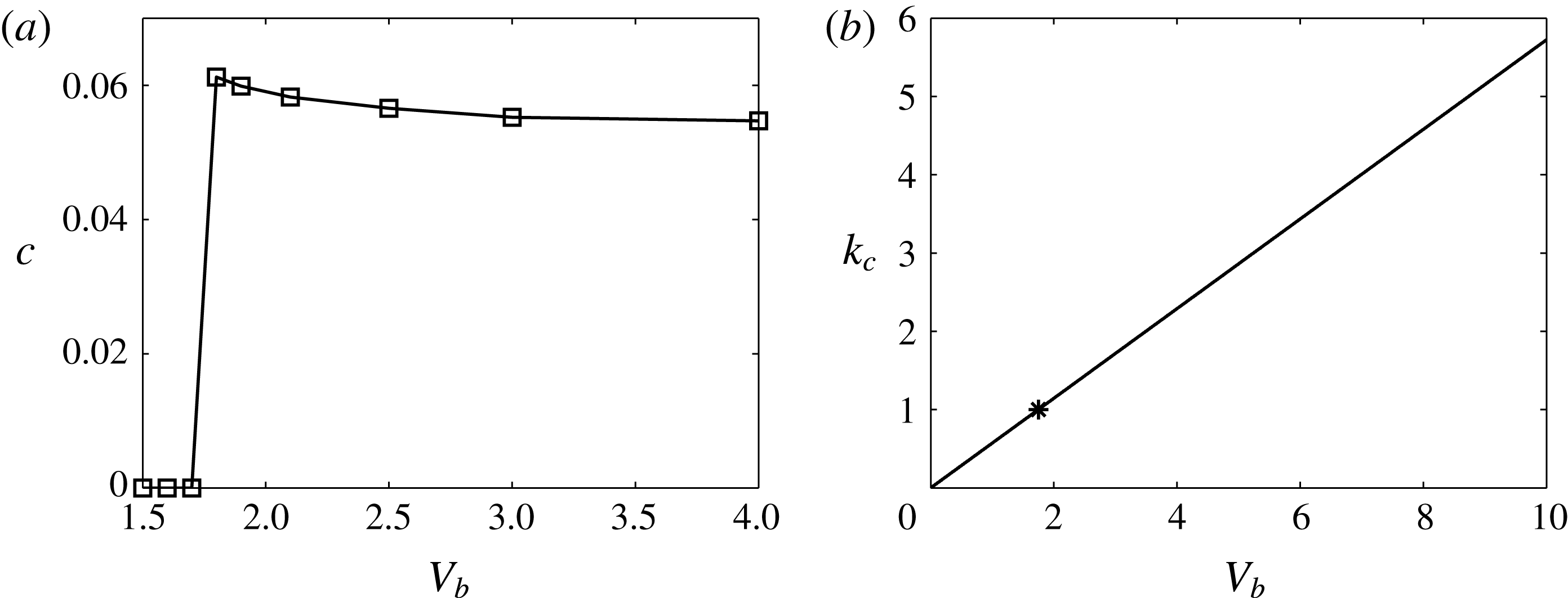
. We quantify the solutions by estimating a wave speed
 $c$
that measures the streamwise motion of the interfacial wave – the solution is not exactly a travelling wave of permanent form – it is time-periodic and travelling. This is done by following trajectories in the
 $x$
–
 $t$
plane of given points on the interface and defining a speed by estimating the slope of given trajectories using least-squares regression. The results are given in figure 6(a) and it is seen that a bifurcation from stationary non-uniform steady-state waves to travelling modulated waves takes place at a critical value
 $V_{b}\approx 1.75$
. A direct comparison with the flat-case linear theory is possible from the critical stability curve in
 $k_{c}$
–
 $V_{b}$
space depicted in figure 6(b); in fact we find that
 $k_{c}$
varies linearly with
 $V_{b}$
and at
 $k_{c}=1$
the critical value
 $V_{crit}$
above which instability occurs is given by
 $V_{crit}=1.75$
, in complete agreement for the bifurcation value from steady to time-modulated travelling waves for wavy walls. We conclude that there is a direct correlation between the stability of the flat- and wavy-wall cases; the critical voltage
 $V_{crit}$
found for the flat case corresponds to the value
 $V_{b}$
that marks the transition from steady-state solutions to time-modulated travelling waves.
(a) Estimated interfacial wave speeds
 $c$
for flows over a sinusoidal boundary with
 $d_{b}=0.1$
,
 $k_{b}=1$
and
 $Z_{c}=0.9$
. (b) Neutral stability curve showing the critical wavenumber
 $k_{c}$
as a function of
 $V_{b}$
from linear theory with a flat bottom wall. The star corresponds to wavenumber
 $k_{c}=1$
and
 $V_{crit}=1.75$
. The relative permittivities are
 $\bar{\unicode[STIX]{x1D716}}_{1}=1$
and
 $\bar{\unicode[STIX]{x1D716}}_{2}=5$
and the flow rate is
 $\tilde{Q}=0.1$
.
4.1 Non-uniform steady states for different wall amplitudes
The transition between the two different types of solutions for the wavy-boundary problem was described above and quantified using linear theory for flat walls. We now focus on calculating steady states of the evolution equation (2.32) by solving
 $$\begin{eqnarray}\displaystyle \left\{\frac{D_{3}}{6m_{2}}\left[D_{4}p_{2x}^{(0)}+3m_{2}f_{2}\right]\right\}_{x}=0. & & \displaystyle\end{eqnarray}$$
Equation (4.2) is solved using centred finite differences to discretise derivatives and a Newton–Kantorovich method to solve the resulting set of nonlinear algebraic equations. As a check the solutions were compared with those given by the time-dependent code at least for values of
 $V_{b}<V_{crit}$
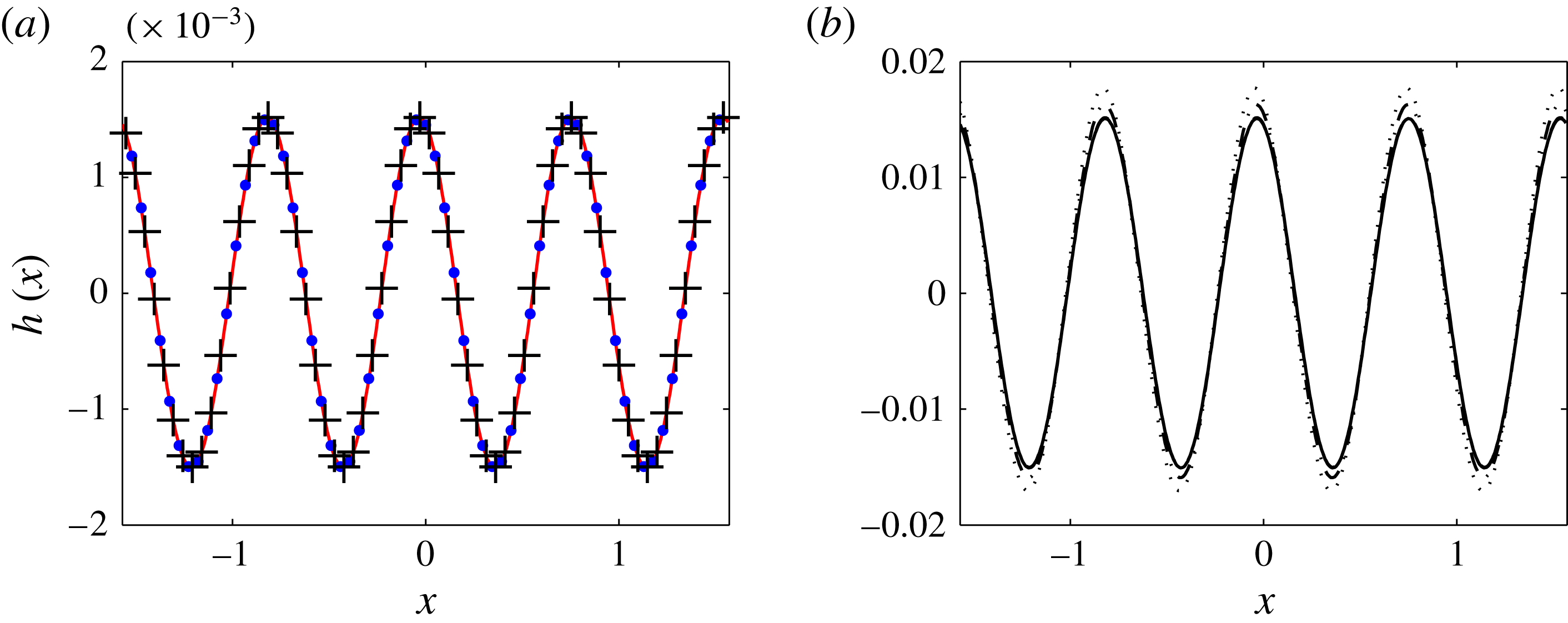
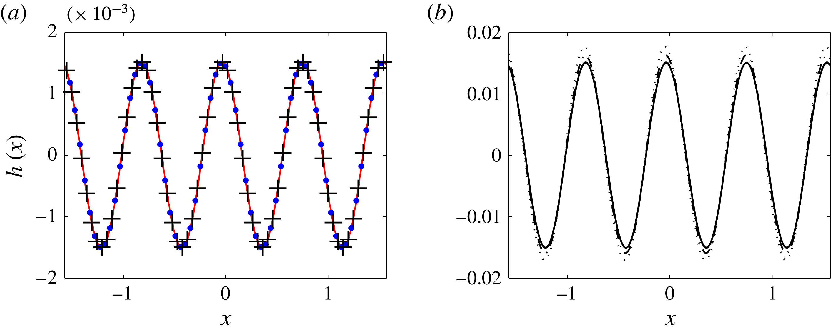
where the solutions are stable – for completeness this is included in figure 7(a) for
 $d_{b}=0.1$
,
 $k_{b}=4$
,
 $\tilde{Q}=0.1$
and
 $V_{b}=3$
, and it is seen that agreement is excellent.
4.2 Analytical solution for small wall waviness
(a) Comparison between the full time-dependent numerical solution (solid curve), the numerical solution of the steady-state ODE (crosses) and the analytical solution (dots with (4.4)) with wall amplitude
 $\unicode[STIX]{x1D700}=0.1$
. (b) Comparison between the analytical solution (solid curve with (4.4)) and the numerical solutions
 $h(x)/\unicode[STIX]{x1D700}$
for
 $\unicode[STIX]{x1D700}=0.1$
(dashed curve),
 $\unicode[STIX]{x1D700}=0.2$
(dot-dashed curve) and
 $\unicode[STIX]{x1D700}=0.3$
(dotted curve). Same parameters as in figure 5(a).
The steady states presented in § 4.1 were calculated numerically for arbitrary wall waviness and in what follows we proceed analytically and construct asymptotic solutions valid for small wall perturbations. We can do this by writing the lower wall as
 $z(x)=Z_{c}+\unicode[STIX]{x1D700}Z(x)$
where
 $\unicode[STIX]{x1D700}\ll 1$
, and looking for an asymptotic solution of the form
 $h(x)=\unicode[STIX]{x1D700}H_{0}(x)+O(\unicode[STIX]{x1D700}^{2})$
. Substituting these into (4.2) gives, to leading order,
 $$\begin{eqnarray}\displaystyle AH_{0}+BH_{0x}+CH_{0xxx}=-DZ-EZ_{x}, & & \displaystyle\end{eqnarray}$$
where
 $A$
,
 $B$
,
 $C$
,
 $D$
and
 $E$
are constants that depend on the physical parameters in the problem (they are found as needed by using the symbolic manipulator Maple). To fix things, we proceed with a sinusoidal wall perturbation of wavelength
 $2\unicode[STIX]{x03C0}/k_{b}$
and specifically take
 $Z(x)=-\text{cos}(k_{b}x)$
in order to enable comparisons with nonlinear steady states computed for wavy wall perturbations given by (4.1). It follows that the general solution of (4.3) is given by
 $$\begin{eqnarray}\displaystyle H_{0}(x)=\mathop{\sum }_{i=1}^{3}C_{i}\text{e}^{\unicode[STIX]{x1D706}_{i}x}+C_{4}+\text{Re}(p)\cos (kk_{b}x)-\text{Im}(p)\sin (kk_{b}x), & & \displaystyle\end{eqnarray}$$
where
 $C_{i}$
,
 $i=1,2,3,4$
, are constants and
 $\unicode[STIX]{x1D706}_{i}$
,
 $i=1,2,3$
, are the roots of
 $A+B\unicode[STIX]{x1D706}+C\unicode[STIX]{x1D706}^{3}=0$
. The complex number
 $p$
is given by
 $$\begin{eqnarray}p=\frac{D+\text{i}kk_{b}E}{A+\text{i}kk_{b}B-\text{i}(kk_{b})^{3}C}.\end{eqnarray}$$
The constants
 $C_{i}$
, corresponding to the homogeneous solution, are found by imposing periodic boundary conditions over
 $x\in [-\unicode[STIX]{x03C0}/k,\unicode[STIX]{x03C0}/k]$
and the conservation of mass integral constraint on
 $H_{0}$
,
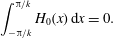 $$\begin{eqnarray}\displaystyle \int _{-\unicode[STIX]{x03C0}/k}^{\unicode[STIX]{x03C0}/k}H_{0}(x)\,\text{d}x=0. & & \displaystyle\end{eqnarray}$$
In the special case when
 $k_{b}$
and
 $k$
are integers with
 $k_{b}\neq \unicode[STIX]{x1D706}_{i}$
for
 $i=1,2,3$
, it can be shown that the roots of
 $A+B\unicode[STIX]{x1D706}+C\unicode[STIX]{x1D706}^{3}=0$
are such that
 $\text{Re}(\unicode[STIX]{x1D706})\neq 0$
and hence the homogeneous contribution to the solution cannot be spatially periodic. In such cases, the expression for the interface simplifies to
 $$\begin{eqnarray}\displaystyle H_{0}(x)=\text{Re}(p)\cos (kk_{b}x)-\text{Im}(p)\sin (kk_{b}x), & & \displaystyle\end{eqnarray}$$
which can be interpreted as a phase shift in the interface position relative to the wall. In figure 7(a) we superimpose the leading-order analytical solution (4.7) with
 $\unicode[STIX]{x1D700}=0.1$
along with the full time-dependent numerical solution integrated to steady state, and the numerical solution of (4.2). Figure 7(b) considers larger wall amplitudes
 $\unicode[STIX]{x1D700}=0.2$
and
 $0.3$
and it can be seen that the leading-order solution (4.7) is reasonably accurate even beyond its expected range of validity. Note that inclusion of
 $\unicode[STIX]{x1D700}^{2}$
corrections is expected to improve the agreement as found in the related studies of falling films over topography (e.g. Tseluiko et al.
Reference Tseluiko, Blyth, Papageorgiou and Vanden-Broeck2008).
4.3 Large-amplitude sinusoidal boundary
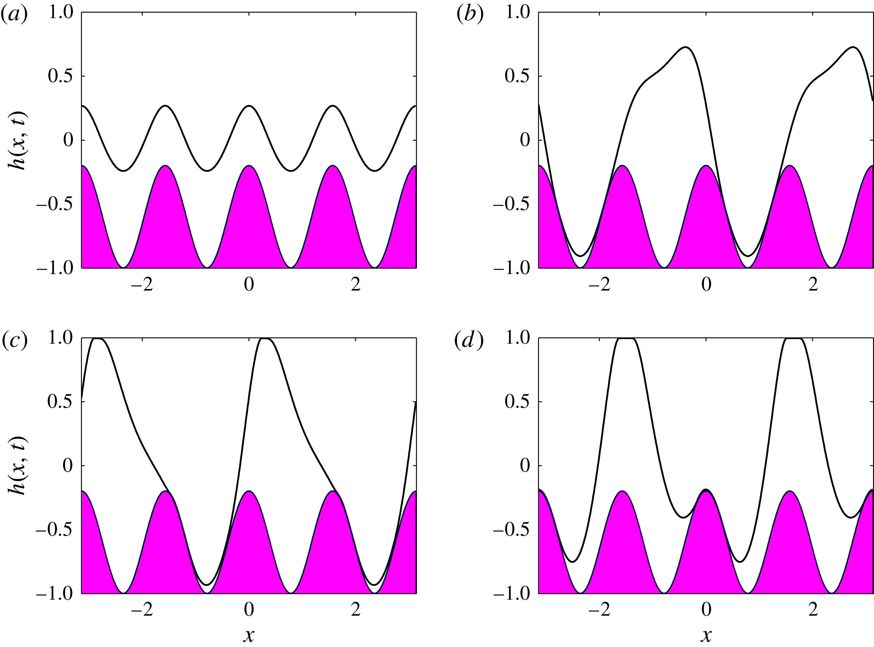
Interface
 $h(x,t)$
at final times (a)
 $t=50$
, (b)
 $t=100$
, (c)
 $t=152$
and (d)
 $t=200$
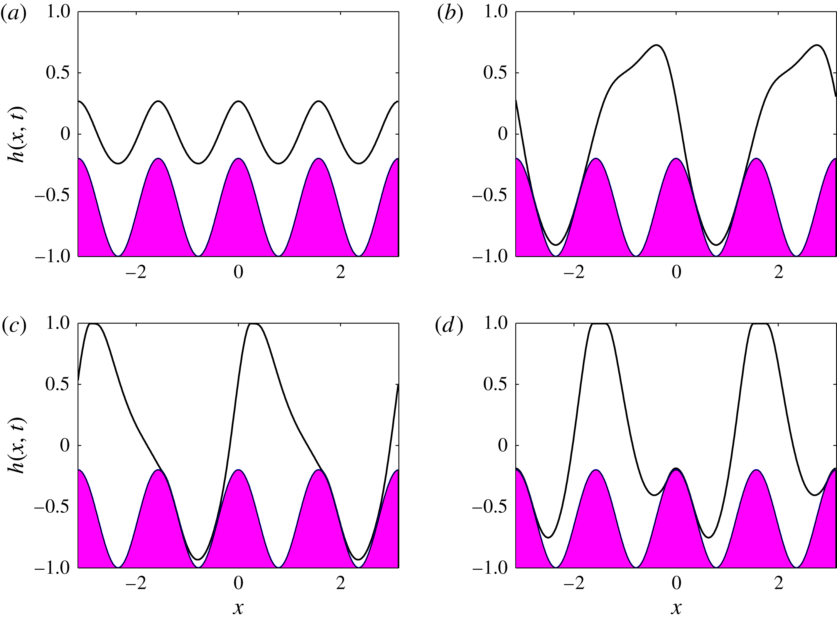
. Other parameters are
 $V_{b}=7$
,
 $\tilde{Q}=0.0345$
,
 $d_{b}=0.4$
,
 $k_{b}=4$
,
 $Z_{c}=0.6$
,
 $\unicode[STIX]{x1D6FD}=1$
,
 $\bar{\unicode[STIX]{x1D716}}_{1}=1$
,
 $\bar{\unicode[STIX]{x1D716}}_{2}=2$
and
 $m_{2}=1$
.
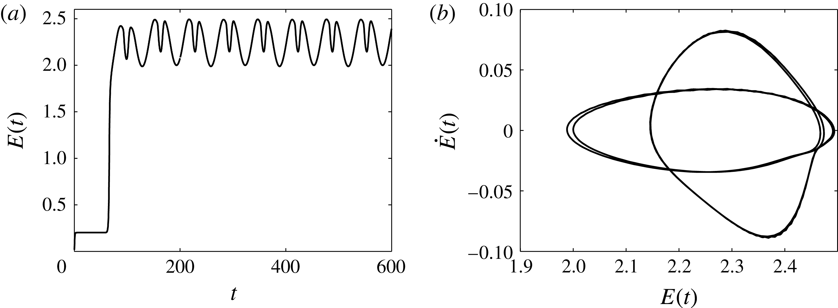
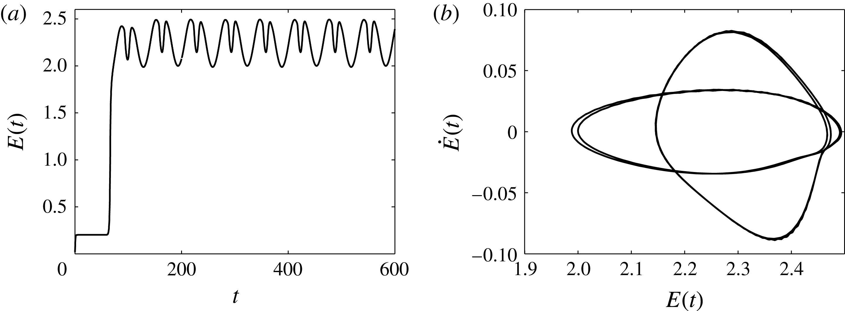
(a) Time evolution of the energy
 $E(t)$
of the solution presented in figure 8. (b) Phase plane of the energy,
 $E$
versus
 $\text{d}E/\text{d}t$
, for times between
 $t=200$
and
 $t=600$
.
In this section we examine the flow through highly constricted channels with wavy boundaries that occupy nearly half of the channel width. In the computations described next, the initial condition is chosen to be
 $h(x,0)=0$
. For weak fields or in the absence of a field altogether, we would expect to reach the non-uniform steady states given by solutions of (4.2). For large wall amplitudes, an additional physical feature of the steady states is the formation of vortices in the troughs that are now deep enough to accommodate them – see below for numerical results. For related single-phase problems, such as falling films over sinusoidally corrugated walls, see the experiments of Pollak & Aksel (Reference Pollak and Aksel2013). At large enough values of the voltage parameter
 $V_{b}$
, the unsteady numerical simulations predict that the interface initially reaches a steady state, but eventually instability sets in, with the dynamics transitioning to what we have termed ‘walking behaviour’. This behaviour can be mainly characterised by three stages: first the flow loses stability and parts of the interface get attracted to the lower wavy wall and other parts to the flat upper wall; this transient stage continues with the interface going into the troughs and over the crests in very close proximity to the wavy wall, with regions ahead (or behind) reaching the upper wall; finally the dynamics enters a final state that resembles a travelling wave, parts of which hug the lower wavy wall and other parts the upper wall. It is quite striking to discover that the resulting nonlinear dynamics are time-periodic for a large range of parameters that were studied. Representative computations are provided in figure 8 for
 $V_{b}=7$
,
 $\tilde{Q}=0.0345$
, and a wavy wall with mean position
 $y=-0.6$
, wall amplitude
 $d_{b}=0.4$
and wavenumber
 $k_{b}=4$
. The scaled channel height is
 $y=1$
(
 $\unicode[STIX]{x1D6FD}=1$
) and the scaled relative permittivities are
 $\bar{\unicode[STIX]{x1D716}}_{1}=1$
and
 $\bar{\unicode[STIX]{x1D716}}_{2}=2$
(recall that
 $m_{2}=1$
). Figure 8(a) shows the solution close to its unstable steady state at
 $t=50$
, while figure 8(b–d) at times
 $t=100,152,200$
depicts solutions from the three stages described above. For
 $t>200$
the dynamics enters the time-periodic attractor mentioned earlier and this is quantified further in figure 9, which considers the flow from
 $t=200$
to
 $t=600$
. Figure 9(a) shows the evolution of the energy norm
 $E(t)$
from
 $t=0$
until the final time
 $t=600$
. It is seen that the solution quickly reaches a non-uniform steady state characterised by the constant value
 $E(t)\approx 0.2$
until approximately
 $t=70$
, and then rapidly loses stability to a much higher-energy state that eventually becomes time-periodic. Conclusive evidence of the time periodicity is provided in figure 9(b), which constructs the energy phase plane, which is seen to be a closed curve consisting of four almost congruent loops – inspection of figure 9(a,b) shows that there are four energy minima and four maxima over one period and the period is approximately equal to 130 time units.
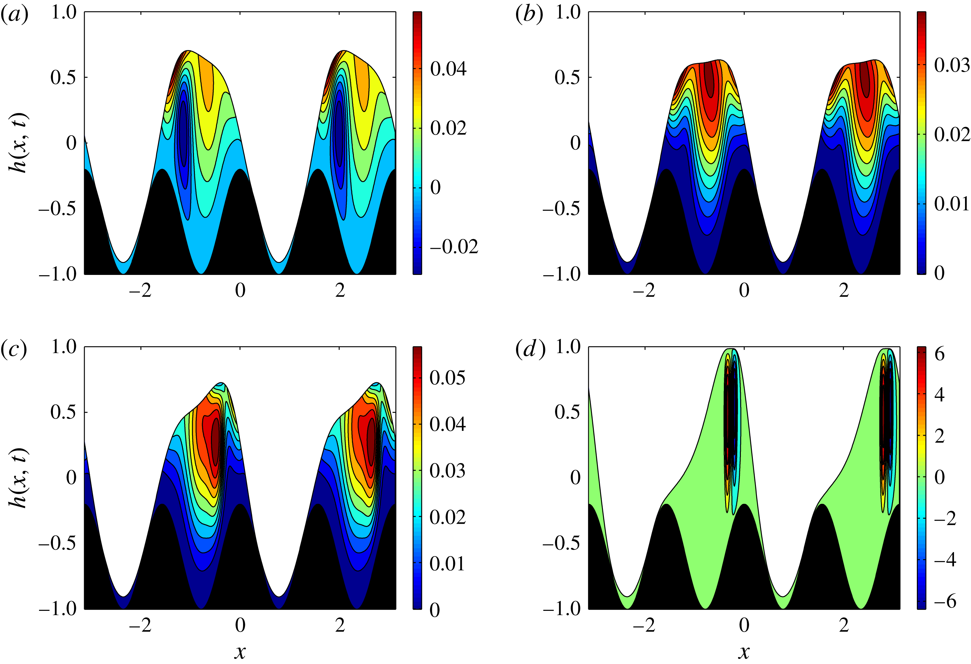
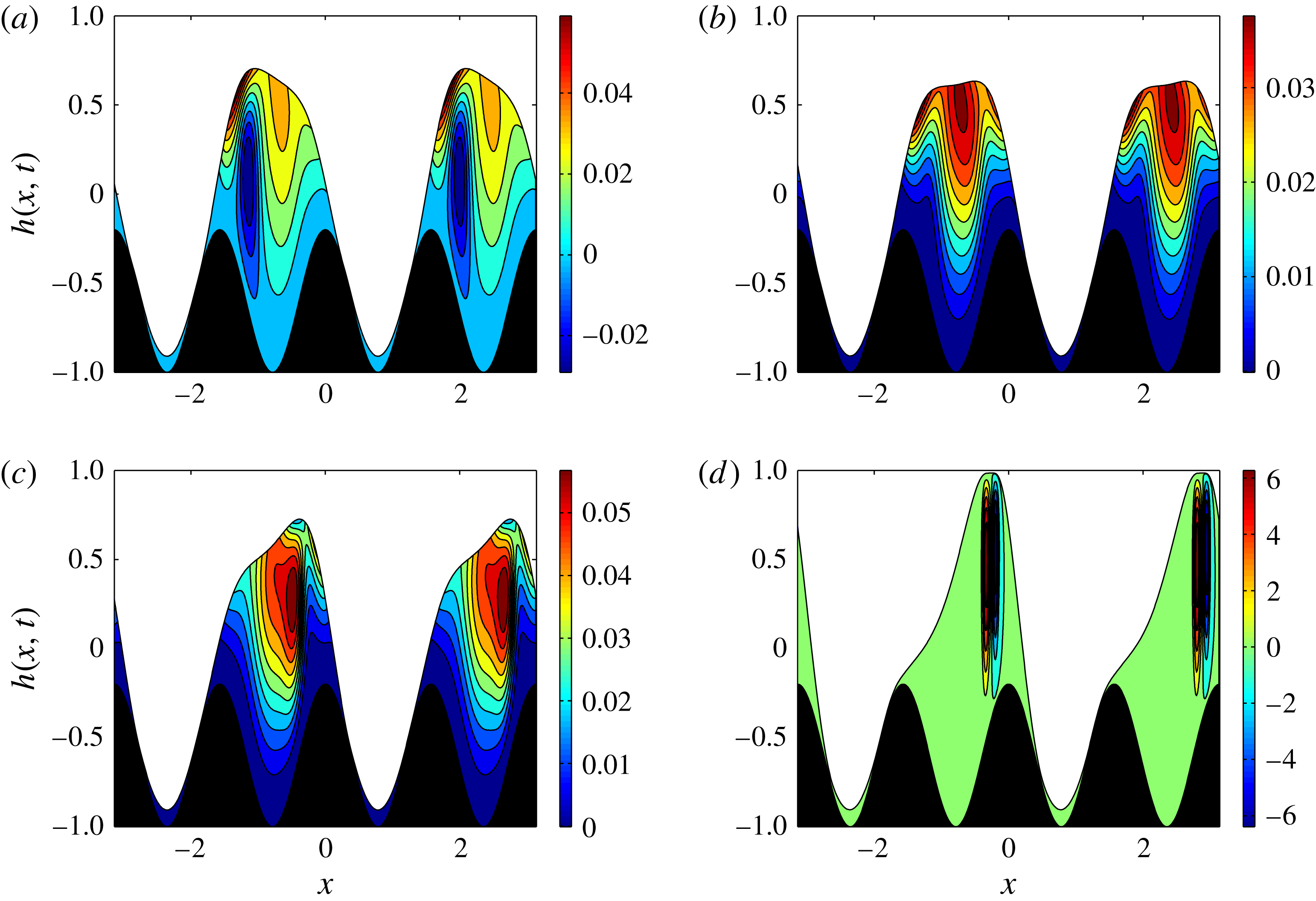
Instantaneous streamlines at (a)
 $t=96$
, (b)
 $t=98$
, (c)
 $t=100$
and (d)
 $t=106$
. All other parameters as in figure 8.
In order to inspect the flow more thoroughly and in particular to obtain insight regarding the vorticity and subsequent mixing capabilities in such systems, we write the fluid velocity in the lower layer (analogously in the upper layer) in terms of the streamfunction
 $\unicode[STIX]{x1D713}(x,y)$
such that
 $u_{2}^{(0)}=\unicode[STIX]{x1D713}_{y}$
and
 $v_{2}^{(0)}=-\unicode[STIX]{x1D713}_{x}$
. We note, however, that we are working within the lubrication approximation and it is likely that this assumption needs to be relaxed in order to obtain accurate recirculation zones and subsequent mixing statistics. Using the expression for the horizontal fluid velocity given by (2.29) readily yields
 $$\begin{eqnarray}\displaystyle \unicode[STIX]{x1D713}(x,y,t)=\frac{p_{2x}^{(0)}}{2m_{2}}\left(\frac{y^{3}}{3}-z(x)^{2}y\right)+f_{2}\left(\frac{y^{2}}{2}+z(x)y\right)+c_{1}(x), & & \displaystyle\end{eqnarray}$$
where
 $c_{1}(x)$
is found by setting
 $\unicode[STIX]{x1D713}(x,-z(x),t)=0$
, i.e. the lower wall is defined to be a zero streamline. Figure 10 provides the instantaneous streamlines of the flow depicted in figure 8, at four consecutive times
 $t=96,98,100,106$
(the bar on the right shows the value of
 $\unicode[STIX]{x1D713}$
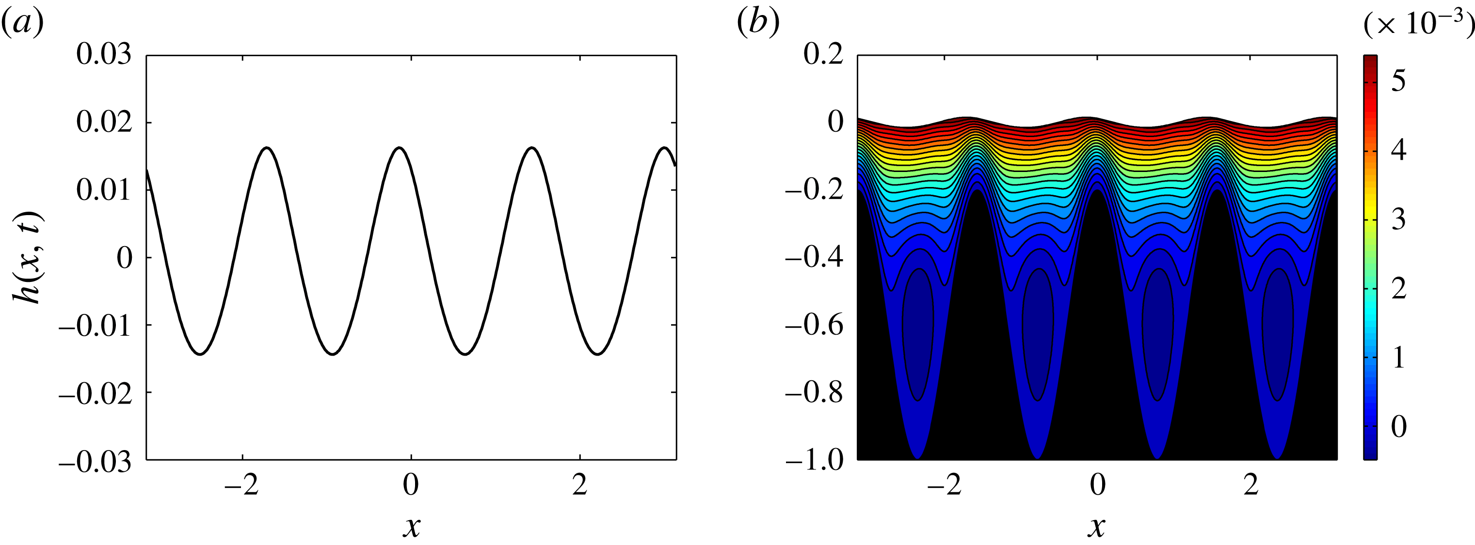
in the contour plots). As described earlier and seen in figure 10, a distinct feature of the flow, at a fixed time, is that parts of the interface are in close proximity to troughs while ahead (behind) of these regions the interface climbs over the hump to reach the upper wall. What is interesting is that every time the interface goes over the wall humps and the lower fluid extends up to the upper wall, two counter-rotating vortices form in close proximity to each other – see for example figure 10(d). As time increases, these vortices get swept along downstream by the flow. We conclude this section by considering the same large-amplitude wavy boundary as above but now take a smaller value
 $V_{b}=2$
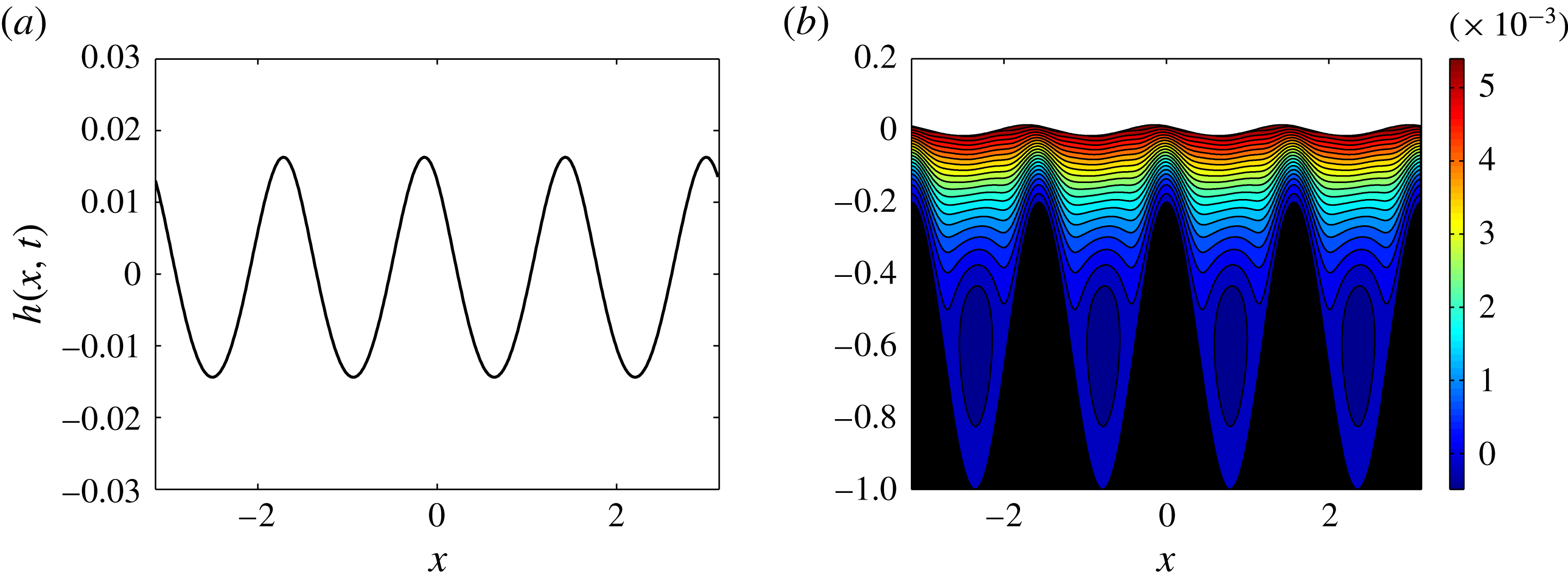
. In such cases the interface reaches a steady state with vortices and flow recirculation taking place in the troughs, with the remaining flow unidirectionally moving over the peaks. Numerical results are given in figure 11 with panel (a) showing the interface at
 $t=100$
after steady state has been reached, and panel (b) showing the streamlines of the corresponding state. The vortices are seen in the troughs and we note that they are fairly weak, with the flow in their vicinity almost stagnant.
The results in this section indicate that, for a given imposed flow rate, the wall geometry and electric field can be manipulated to obtain dynamical behaviour in confined microscale geometries that may be useful in applications. The dynamics arise due to loss of stability of non-uniform steady states, and in what follows we consider such questions using linear Floquet analysis.
(a) Interface
 $h(x,t)$
and (b) streamlines at time
 $t=100$
. Parameters are the same as in figure 8 but with a different voltage
 $V_{b}=2$
.
5 Floquet stability analysis of non-uniform flows
The objective of this section is to use linear stability theory to establish ranges of values of
 $V_{b}$
for which the flow transitions from non-uniform steady states to the ‘walking behaviour’ we described in the previous section. A natural setting for the analysis is to use Floquet theory since the underlying flows are spatially periodic. Given a steady state
 $h_{s}(x)$
that solves (4.2), we write
 $h(x,t)=h_{s}(x)+\tilde{h}(x,t)$
, substitute into (2.32) and linearise to obtain
 $$\begin{eqnarray}\displaystyle \tilde{h}_{t}+[f_{1}\tilde{h}+f_{2}\tilde{h}_{x}+f_{3}\tilde{h}_{xxx}]_{x}=0, & & \displaystyle\end{eqnarray}$$
where
 $f_{i}=f_{i}(h_{s},h_{sx},h_{sxxx},z,z_{x})$
for
 $i=1,2,3$
are periodic functions of
 $x$
with the same period as the steady-state solution, and they are found using Maple. Looking for solutions of the form
 $$\begin{eqnarray}\tilde{h}(x,t)=F(x)\exp (\unicode[STIX]{x1D706}t+\text{i}kx),\end{eqnarray}$$
where
 $F(x)$
is a periodic function with the same spatial period as
 $\tilde{h}(x,t)$
and the eigenvalue
 $\unicode[STIX]{x1D706}$
is complex, (5.1) becomes
 $$\begin{eqnarray}\displaystyle & & \displaystyle \unicode[STIX]{x1D706}F+F\left[f_{1x}+\text{i}k(f_{1}+f_{2x}-k^{2}f_{2}-\text{i}k^{3}f_{3x}+k^{4}f_{3})\right]\nonumber\\ \displaystyle & & \displaystyle \quad +\,F^{\prime }\left[f_{1}+f_{2x}+2\text{i}kf_{2}-3k^{2}f_{3x}-4\text{i}k^{4}f_{3}\right]\nonumber\\ \displaystyle & & \displaystyle \quad +\,F^{\prime \prime }\left[f_{2}+3\text{i}kf_{3x}-6k^{2}f_{3}\right]+F^{\prime \prime \prime }\left[f_{3x}+4\text{i}kf_{3}\right]+F^{\prime \prime \prime \prime }\left[f_{3}\right]=0.\end{eqnarray}$$
In the calculations that follow we consider perturbations of the same wavelength as the underlying solution, and so set
 $k=0$
in (5.3) – a full parametric study for arbitrary
 $k$
would be interesting but is omitted here for brevity. If instability is found for
 $k=0$
, then we surmise that it will be present for a range of non-zero
 $k$
also, since the flow is long-wave unstable. On the other hand, if
 $\text{Re}(\unicode[STIX]{x1D706})<0$
for
 $k=0$
, then we cannot conclude that the flow is stable for all
 $k$
without carrying out additional calculations. In the results that follow, stability or instability is based on the calculations for
 $k=0$
. In what follows, we analyse a typical case having flow rate
 $\tilde{Q}=0.1$
, and sinusoidal lower wall topography of amplitude
 $d_{b}=0.4$
, wavenumber
 $k_{b}=4$
and mean value
 $y=-Z_{c}=-0.6$
; other parameters are as before with
 $\unicode[STIX]{x1D6FD}=1$
,
 $\bar{\unicode[STIX]{x1D716}}_{1}=1$
,
 $\bar{\unicode[STIX]{x1D716}}_{2}=2$
and
 $m_{2}=1$
. Keeping these parameters fixed, we vary the voltage
 $V_{b}$
and compute the eigenvalues
 $\unicode[STIX]{x1D706}$
numerically. For each
 $V_{b}$
we find
 $n$
eigenvalues, where
 $n$
is the number of discretisation points in
 $x$
. Derivatives of
 $F(x)$
are found using spectral differentiation matrices. Since we are essentially interested in detecting instability as
 $V_{b}$
varies, we found it useful to track only those eigenvalues whose real part is sufficiently large, and used
 $\text{Re}(\unicode[STIX]{x1D706})>-0.4$
.
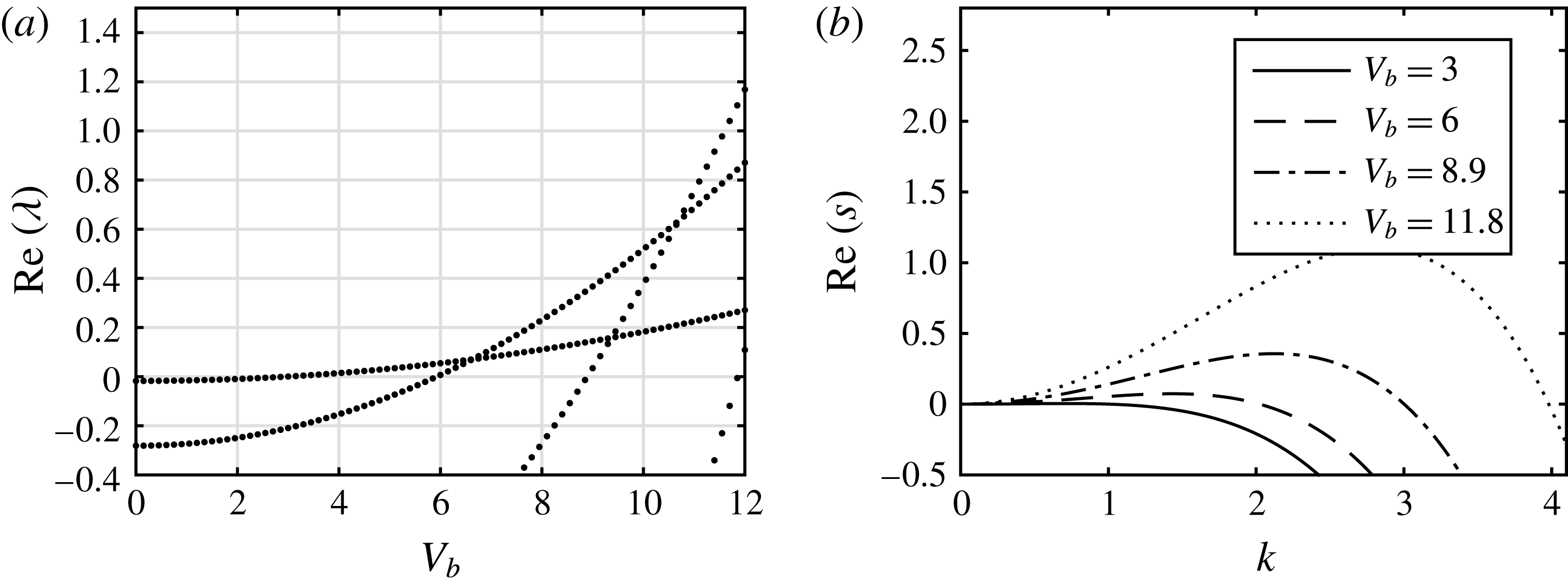
(a) Real part of the growth rate
 $\unicode[STIX]{x1D706}$
as the applied voltage
 $V_{b}$
is varied for a flat boundary case. (b) Real part of the growth rate
 $s$
versus wavenumber
 $k$
as calculated from the linear stability analysis in § 2.4 for
 $V_{b}=3$
(solid line),
 $V_{b}=6$
(dashed line),
 $V_{b}=8.9$
(dot-dashed line) and
 $V_{b}=11.8$
(dotted line). Other parameters are
 $\tilde{Q}=0.1$
,
 $\unicode[STIX]{x1D6FD}=1$
,
 $\bar{\unicode[STIX]{x1D716}}_{1}=1$
,
 $\bar{\unicode[STIX]{x1D716}}_{2}=2$
and
 $m_{2}=1$
.

The code was tested for the trivial case of a flat wall, and hence
 $h_{s}(x)=0$
, against the results given in § 2.4. In the Floquet setting of this problem, we need to solve
 $$\begin{eqnarray}\displaystyle \unicode[STIX]{x1D706}F+AF_{x}+BF_{xx}+CF_{xxxx}=0, & & \displaystyle\end{eqnarray}$$
where
 $A$
,
 $B$
and
 $C$
are the same constants as the ones found in (4.3). The calculated real part of
 $\unicode[STIX]{x1D706}$
versus
 $V_{b}$
is given in figure 12(a) where, as noted above, only eigenvalues greater than
 $-0.4$
are shown. The results show different modes and how they become unstable as
 $V_{b}$
increases. The first mode becomes unstable when
 $V_{b}=3$
, and then there are subsequent crossings by the second mode at
 $V_{b}=6$
, the third at
 $V_{b}=8.9$
and the fourth at
 $V_{b}=11.8$
. Figure 12(b) shows the growth rate as a function of wavenumber for different
 $V_{b}$
as found in § 2.4. The values of
 $V_{b}$
above which the modes
 $k=1,2,3,4$
become successively unstable are confirmed to be the same as those found using the Floquet analysis.
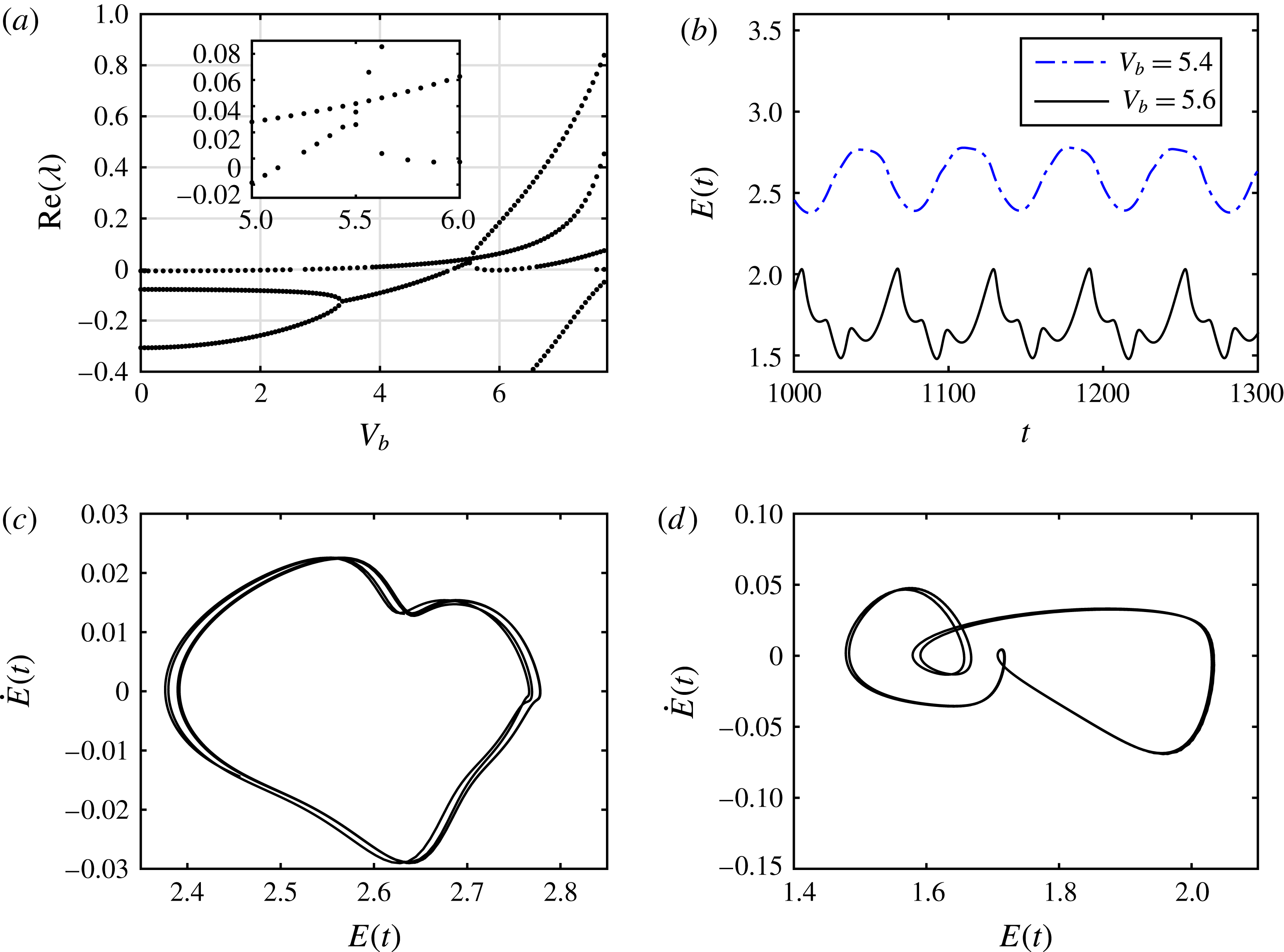
(a) Real part of the growth rate
 $\unicode[STIX]{x1D706}$
versus applied voltage
 $V_{b}$
. Same parameters as in figure 12 with
 $d_{b}=0.4$
,
 $k_{b}=4$
and
 $Z_{c}=0.6$
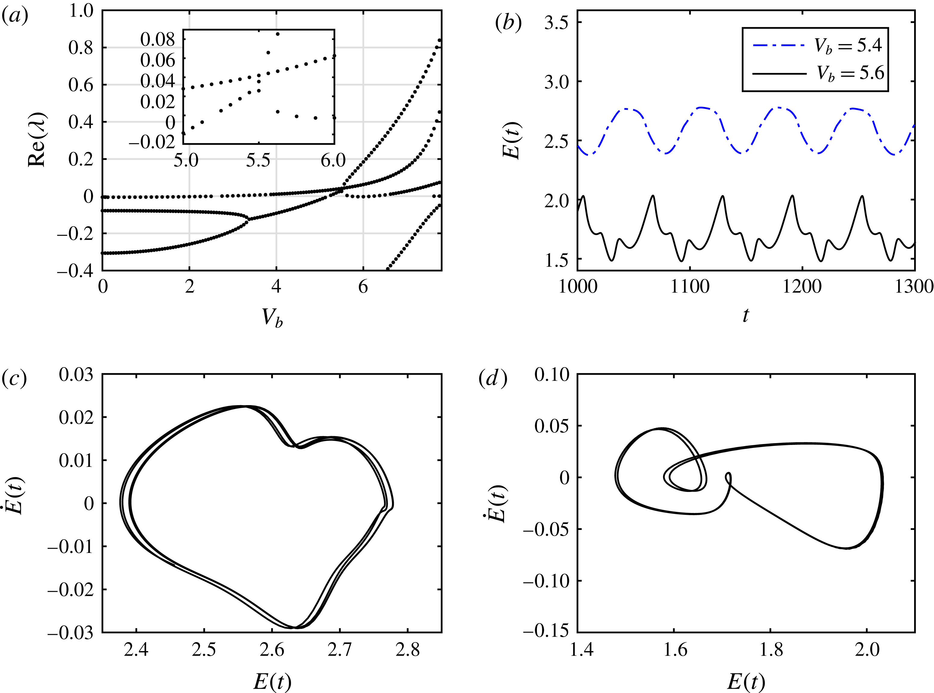
. (b) Time evolution of the energy
 $E(t)$
. Applied voltage is
 $V_{b}=5.4$
(dot-dashed line) and
 $V_{b}=5.6$
(solid line). The lower panels show the phase plane of the energy for (c)
 $V_{b}=5.4$
and (d)
 $V_{b}=5.6$
. Simulations of interfacial evolution for
 $V_{b}=5.4$
and
 $V_{b}=5.6$
can be found in supplementary movies 2 and 3, respectively.
Next we consider the case with a wavy boundary and parameters as given above, and compute the eigenvalues
 $\unicode[STIX]{x1D706}$
from (5.3) with
 $k=0$
. Figure 13(a) shows the variation of the real part of
 $\unicode[STIX]{x1D706}$
with
 $V_{b}$
; note that the first crossing yielding instability occurs at
 $V_{b}=2.6$
. This has been confirmed from the nonlinear time-dependent computations that predict stability of non-uniform states for these parameters when
 $V_{b}<2.6$
. The next mode crossing to become unstable occurs at around
 $V_{b}=5.2$
. Some intricate behaviour is found near this point and the inset in figure 13(a) depicts branches in more detail. It is seen that the branch that crossed at
 $V_{b}\approx 5.2$
itself pitchfork bifurcates at
 $V_{b}\approx 5.5$
into two branches. To observe the differences in the dynamics, we took values
 $V_{b}=5.4$
and
 $V_{b}=5.6$
that are below and above the critical value
 $V_{b}=5.5$
, and ran large-time simulations of the nonlinear initial value problem. We find that the solution transitions into the ‘walking behaviour’ described earlier and the energy norms along with the corresponding phase planes are included in figure 13(b–d). The lower-voltage energy norm is less intricate than that for
 $V_{b}=5.6$
in the sense that it does not contain as high-frequency oscillations. It is also clear from figure 13(b) that the time-averaged energy values are different, and we can conclude that the two solutions are on different branches. More information regarding the dynamics of these solutions are given in the phase planes in figure 13(c,d); even though we cannot state this conclusively, it appears that the dynamics for
 $V_{b}=5.4$
are quasi-periodic in time whereas those for
 $V_{b}=5.6$
are periodic and more analogous to those found earlier (e.g. figure 9).
The results presented in figure 13 are for moderate values of
 $V_{b}\leqslant 8$
. Even though a detailed bifurcation study and the stability of the resulting branches is of intrinsic interest, it is beyond the aims of this work, but we illustrate the richness of expected behaviour by considering several larger values of
 $V_{b}$
. For example, solution of the initial value problem starting from a flat interface (all other parameters as in figure 13) and for a relatively high voltage of
 $V_{b}=20$
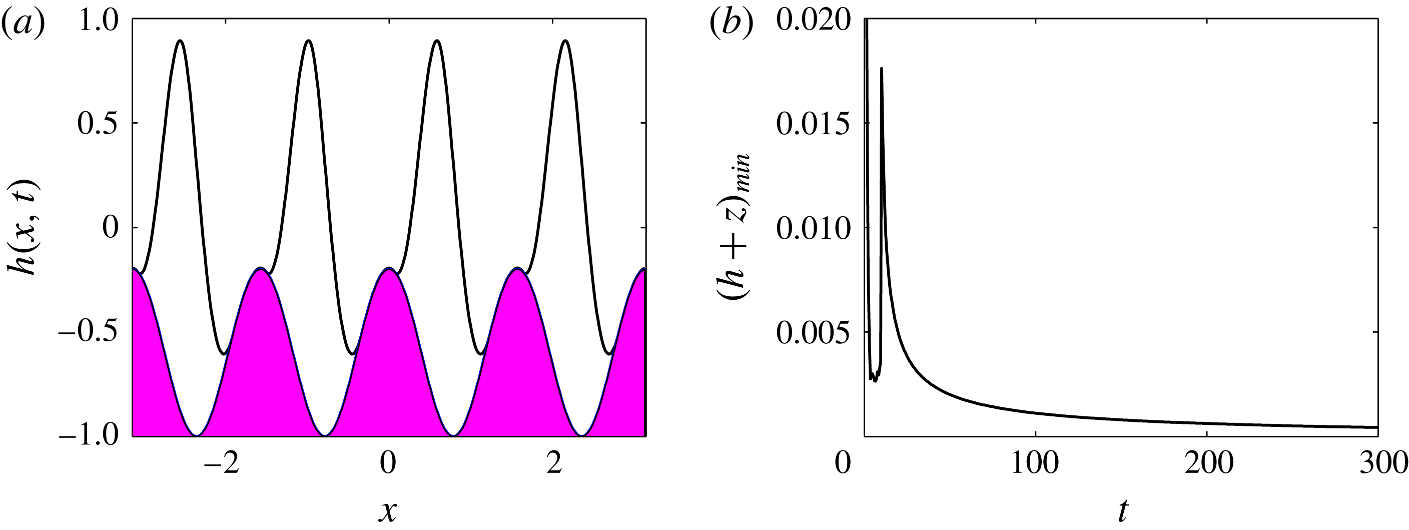
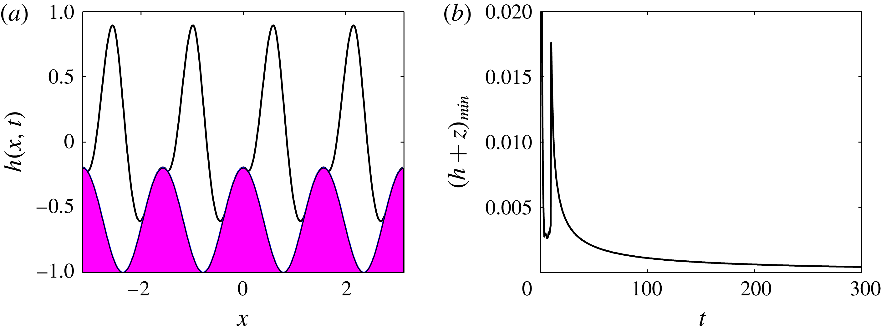
indicates that, after some initial transient oscillations, the system appears to reach a steady state that is stuck at the lower wall troughs but is well separated from the upper wall. Figure 14 shows the solution at a final computed time
 $t_{final}=300$
, and closer inspection of the results shows that the thin films of the lower fluid that form on the wall humps are slowly draining with time. The minimum thickness of these films is plotted against time in figure 14(b) and the slow draining is clearly observed. This solution is another attracting state, albeit quasi-static, and essentially asymptotically traps regions of fluid 2 between successive wall humps with the upper fluid 2 flowing above them, as can be seen from figure 14(a). We note that the simulations indicate that the film thickness does not vanish in finite time in agreement with other related thinning film problems (see e.g. Craster & Matar Reference Craster and Matar2005; Tseluiko & Papageorgiou Reference Tseluiko and Papageorgiou2007b
). (Physically, addition of attracting van der Waals forces would rupture the thin film in finite time (see Erneaux & Davis Reference Erneaux and Davis1993; Savettaseranee et al.
Reference Savettaseranee, Papageorgiou, Petropoulos and Tilley2003).) For
 $V_{b}=8.5$
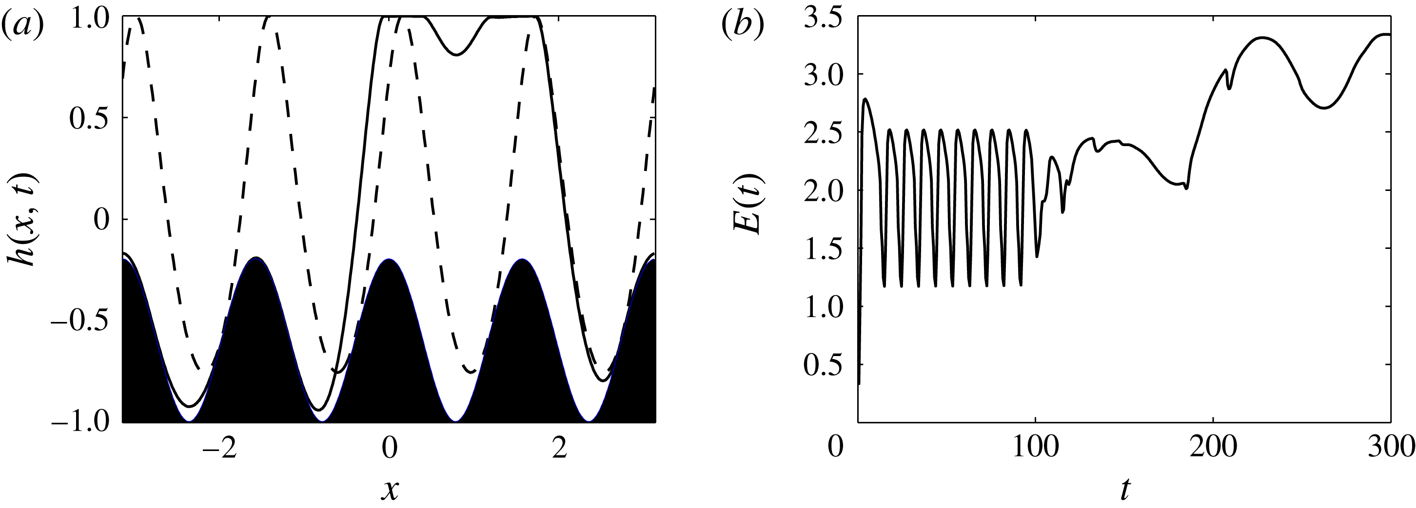
we see the two attracting states competing with each other, with the solution going to the ‘stuck’ behaviour first and then going into a ‘walking’ behaviour. In the former state, the solution undergoes time-periodic oscillations without translating down the channel, before losing stability to the ‘walking’ state. Snapshots of the two solutions are included in figure 16(a) at times
 $t=60$
(dashed curve) and
 $t=300$
(solid curve), along with the evolution of the energy
 $E(t)$
, which indicates the time-periodic behaviour at smaller times and the transition to the ‘walking’ state at larger times. Note that the ‘walking’ state evolves time periodically with a much longer period than that of the ‘stuck’ solution. A movie of the interfacial evolution is also included – see caption of figure 16.
(a) Interface
 $h(x,t)$
at
 $t_{final}=300$
for same parameters as figure 13 and
 $V_{b}=20$
. (b) Minimum of the gap between the interface and the boundary against time.
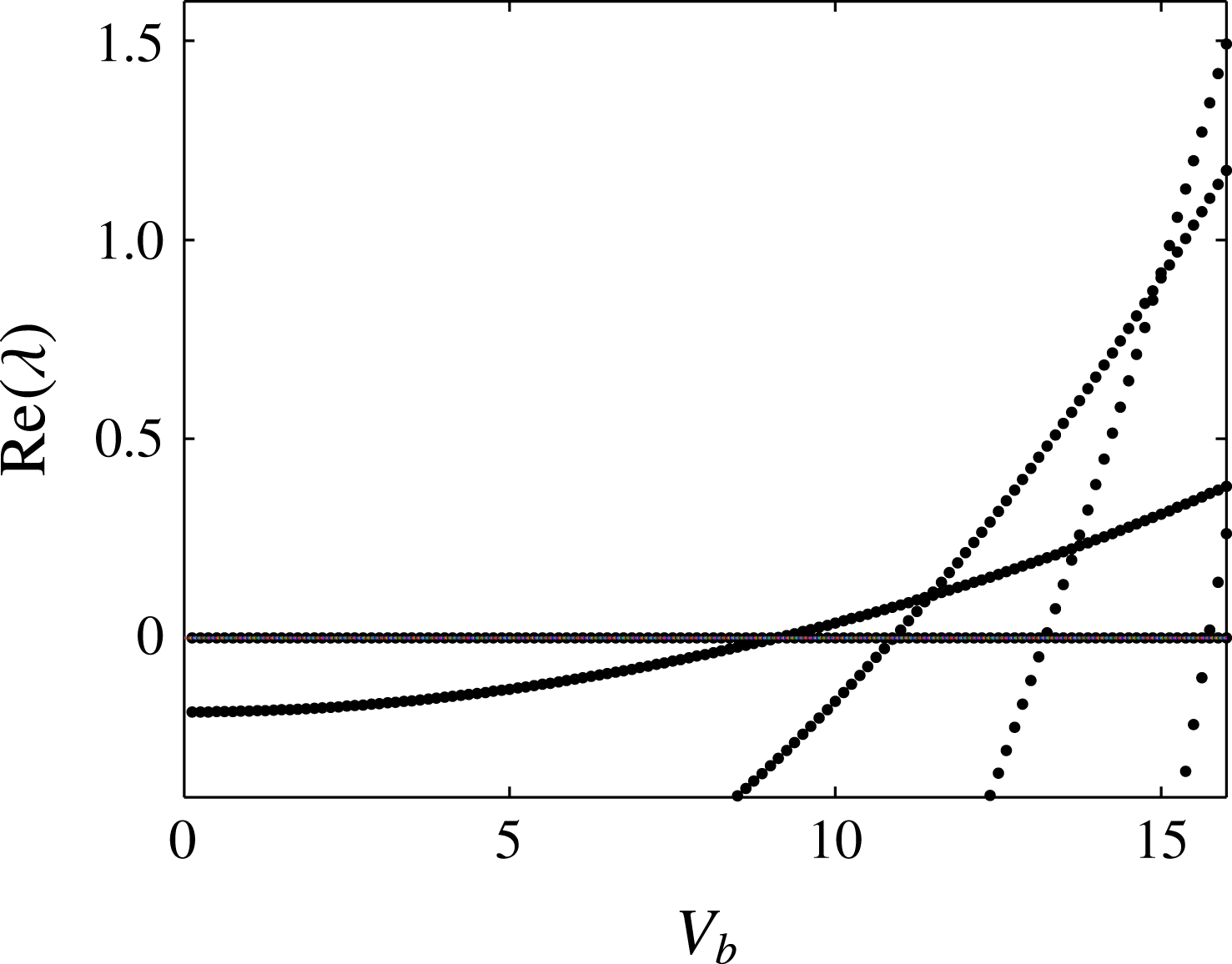
Real part of the growth rate
 $\unicode[STIX]{x1D706}$
versus the applied voltage
 $V_{b}$
. Same parameters as figure 13 but with
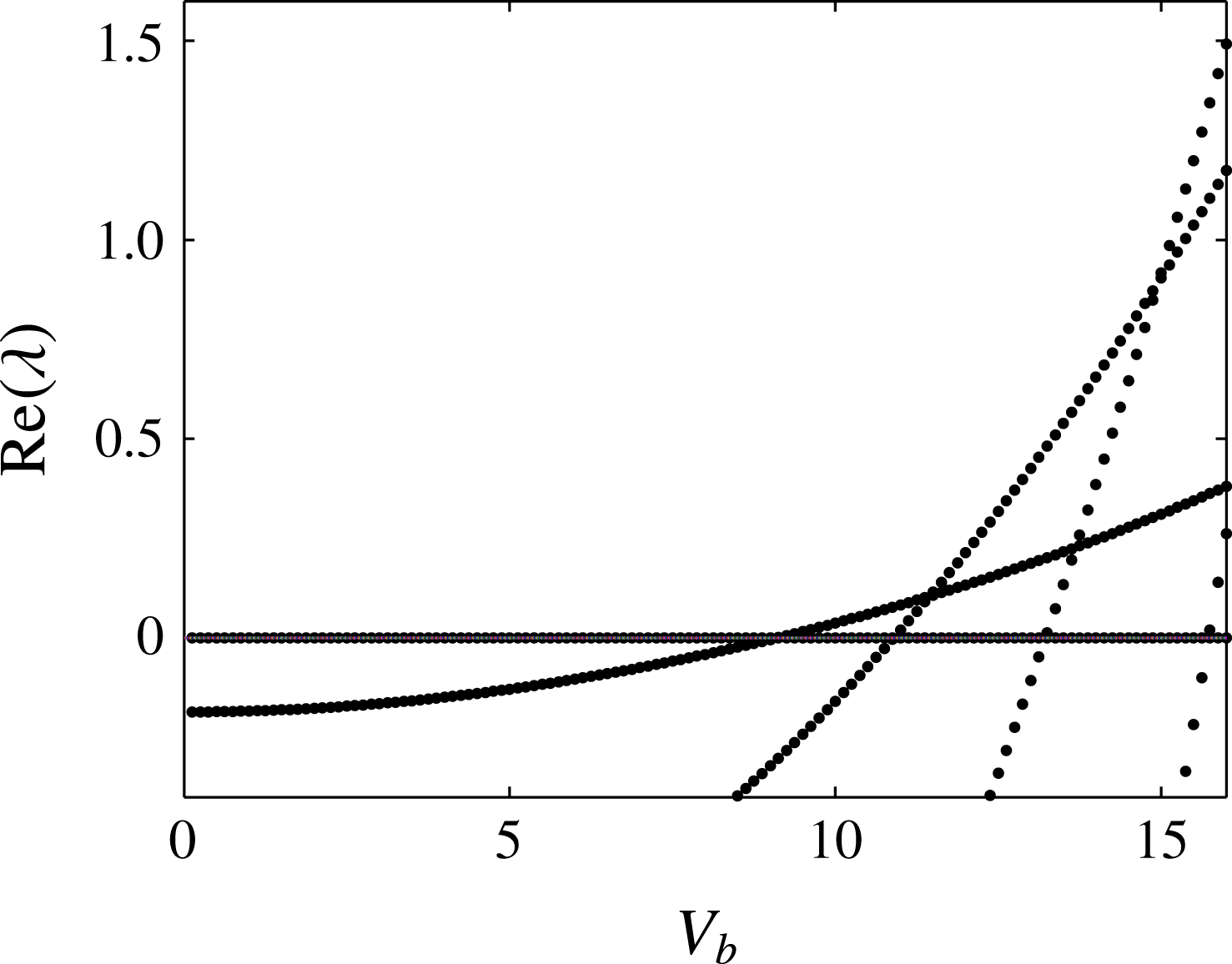
 $\tilde{Q}=20$
.
(a) Interface at times
 $t=60$
(dashed curve) and
 $t=300$
(solid curve) for same parameters as figure 13 and
 $V_{b}=8.5$
. (b) Energy
 $E(t)$
plotted as time is varied. A simulation of the interfacial evolution is given in supplementary movie 4.
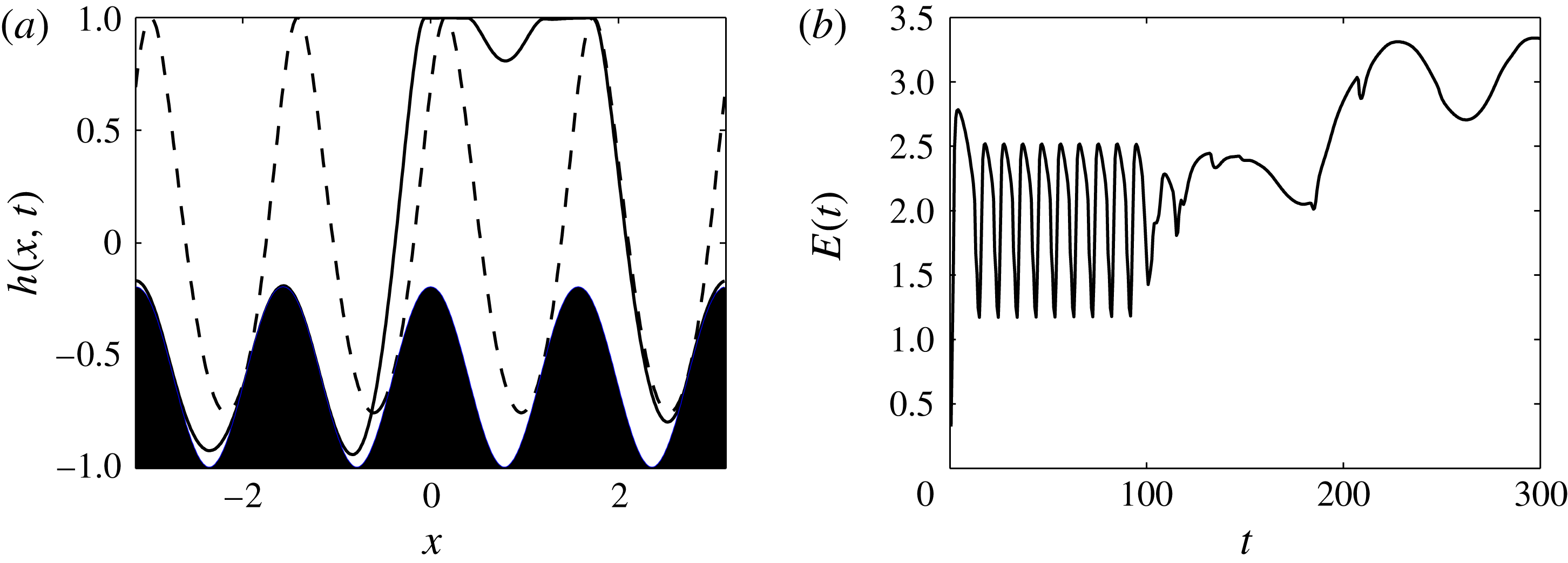
6 Flows at high fluxes
 $\tilde{Q}$

So far we have explored the behaviour of the system for low overall flow rates characterised by small values of
 $\tilde{Q}$
. In this section we consider the behaviour of the confined electrified flow over large-amplitude sinusoidal topography and at relatively large values of
 $\tilde{Q}$
. To fix matters, we consider the same parameters as before (e.g. figure 13) but now take
 $\tilde{Q}=20$
and vary the voltage parameter
 $V_{b}$
.
We begin by considering the linear stability of the non-uniform steady states for
 $\tilde{Q}$
as
 $V_{b}$
varies. The results are shown in figure 15, which depicts the real part of
 $\unicode[STIX]{x1D706}$
for different
 $V_{b}$
. It is found that there is a crossing at
 $V_{b}\approx 9.1$
so that all perturbations with wavelength equal to the domain size are stable for voltages below this value. Comparing these results with those in figure 13 that has
 $\tilde{Q}=0.1$
, we can conclude that generally a higher flow rate has a stabilising effect.
To investigate the dynamics in the unstable regime we pick
 $V_{b}=14$
, which according to the results in figure 15 supports three unstable modes. The initial value problem is solved starting from a flat interface initial condition and following the nonlinear development until
 $t=100$
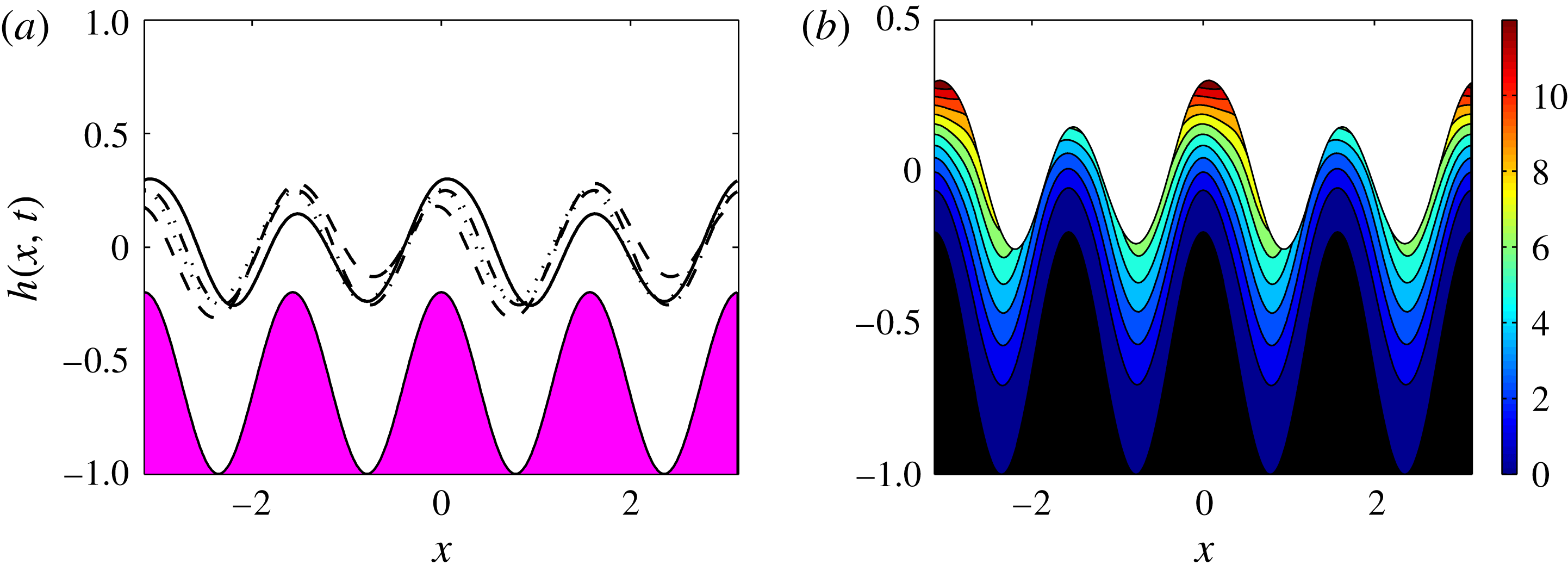
or more. Representative results are given in figure 17. Figure 17(a) shows the interfacial shape at
 $t=1,\,25,\,75$
and
 $100$
, and the results predict clearly that at this moderately large value of
 $\tilde{Q}=20$
the interface mimics the lower wall topography but at the same time performs small-amplitude high-frequency time-dependent oscillations. Figure 17(b) shows the instantaneous streamlines at the final time
 $t=100$
and we can see that the fluid flows over the topography without any vortices present.
(a) Interface
 $h(x,t)$
at
 $t=1$
(dotted line),
 $t=25$
(dot-dashed line),
 $t=75$
(dashed line) and
 $t=100$
(solid line). (b) Streamlines at time
 $t=100$
. Parameters are the same as in figure 8 but with
 $V_{b}=14$
and
 $\tilde{Q}=20$
.
6.1 Asymptotic solution for large
$\tilde{Q}$

The results in figure 17 (as well as several other numerical experiments not reported here) suggest that, as
 $\tilde{Q}$
increases, the flow is a steady state that is modulated spatiotemporally by a small-amplitude and high-frequency component. This observation is now formalised by considering asymptotic solutions to (2.32) for large
 $\tilde{Q}$
. Setting
 $\unicode[STIX]{x1D6FF}=1/\tilde{Q}\ll 1$
, we seek a solution of (2.32) of the form
 $$\begin{eqnarray}\displaystyle h(x,t)=h_{0}(x)+\unicode[STIX]{x1D6FF}H(x,\unicode[STIX]{x1D70F})+\cdots \,,\quad \unicode[STIX]{x1D70F}=t/\unicode[STIX]{x1D6FF}, & & \displaystyle\end{eqnarray}$$
where
 $h_{0}(x)$
is the steady-state solution at these parameter values, i.e. a solution of (4.2). The equation for
 $H(x,\unicode[STIX]{x1D70F})$
emerges at
 $O(\unicode[STIX]{x1D6FF})$
and reads
 $$\begin{eqnarray}\displaystyle H_{\unicode[STIX]{x1D70F}}+\left\{\tilde{F}(h_{0}(x),z(x))H\right\}_{x}=0, & & \displaystyle\end{eqnarray}$$
where
 $\tilde{F}$
is a function of
 $h_{0}(x)$
, the lower boundary shape
 $z(x)$
and its only other dependence is on the physical parameters of the system.
(a) Full numerical solution minus the steady-state solution
 $h(x,t)-h_{0}(x)$
(dashed line) compared with the asymptotic solution
 $\unicode[STIX]{x1D6FF}H(x,\unicode[STIX]{x1D70F})$
(solid line) at four different times with
 $t=\unicode[STIX]{x1D70F}/\tilde{Q}$
. (b) Phase plane of the energy
 $E(t)$
. (c) Plot of
 $E(t)$
as time
 $t$
is varied. (d) Plot of
 $E(\unicode[STIX]{x1D70F})$
as time
 $\unicode[STIX]{x1D70F}$
is varied.
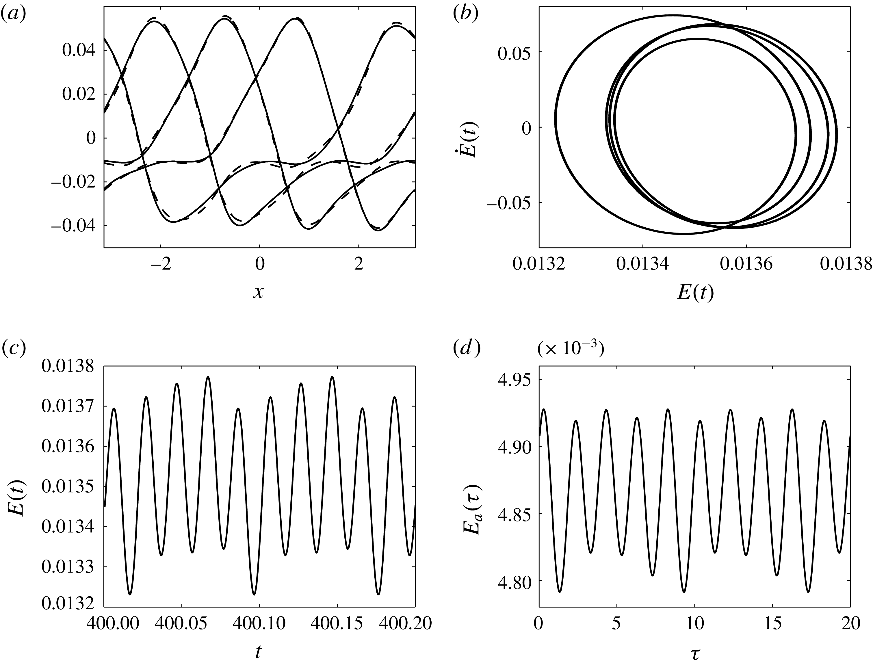
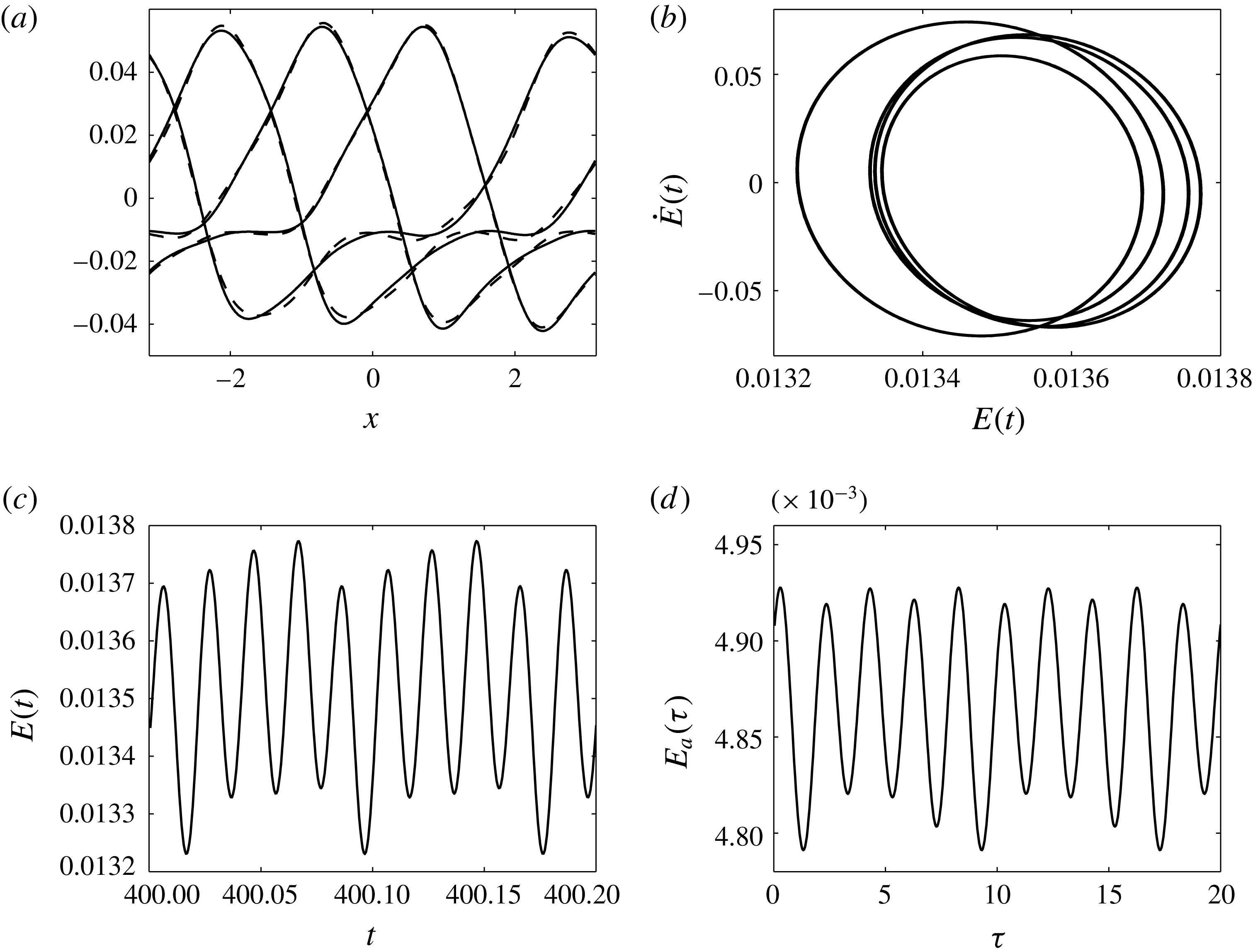
Equation (6.2) is solved numerically for an initial condition given by the full time-dependent numerical solution at a selected time (and after transients have died out) minus the steady state
 $h_{0}(x)$
, and with
 $\tilde{Q}=100$
(so that
 $\unicode[STIX]{x1D6FF}=0.01$
). The asymptotic solution
 $\unicode[STIX]{x1D6FF}H(x,t/\unicode[STIX]{x1D6FF})$
is compared with
 $h(x,t)-h_{0}(x)$
in figure 18(a) for four different times and we see that the agreement between the two is excellent. Figure 18(b) shows the phase plane of the energy of
 $h(x,t)-h_{0}(x)$
coming from the full numerical computation – the spatiotemporal modulation mentioned above is clearly seen from the figure. Figure 18(c) shows the evolution of
 $E(t)$
over approximately 10 oscillation cycles. In figure 18(d) we include the evolution in
 $\unicode[STIX]{x1D70F}$
of the energy
 $E_{a}(\unicode[STIX]{x1D70F})=\int _{-\unicode[STIX]{x03C0}}^{\unicode[STIX]{x03C0}}\unicode[STIX]{x1D6FF}^{2}H^{2}(x,\unicode[STIX]{x1D70F})\,\text{d}x$
of the asymptotic correction, where once again 10 oscillation cycles are included. These data were used to estimate the frequencies
 $f_{t}$
and
 $f_{\unicode[STIX]{x1D70F}}$
of oscillation of the full and asymptotic solutions, respectively. We find that
 $f_{t}/f_{\unicode[STIX]{x1D70F}}\approx 100=\tilde{Q}=1/\unicode[STIX]{x1D6FF}$
as expected. This provides additional evidence of the relevance of the asymptotic solutions at large
 $\tilde{Q}$
. Good agreement was found for
 $\tilde{Q}$
as small as
 $10$
.
7 Conclusions
We have examined the stability and nonlinear dynamics of electrified pressure-driven two-fluid flows in channels with non-uniform cross-sections. A nonlinear evolution equation is derived and studied to describe the nonlinear dynamics of the flow. The system is parametrised by several physical parameters, including the flow rate, the strength of the applied electric field, and the viscosity and permittivity ratios. In addition, the geometry is described by the mean position of the sinusoidal amplitude and wavelength of the lower channel wall, and the position of the upper wall. The upper wall position and the viscosity ratio are set to unity in order to reduce the number of parameters.
Our main objective is the detailed study of the effect of imposed flow and electric fields on the nonlinear dynamics for both flat and undulating channel walls. For flat walls it is shown that the electric field destabilises the flow as observed in linear studies in the literature. As the instability grows nonlinearly to large amplitudes and towards the walls, it is prevented from touching by the imposed flow measured by our parameter
 $\tilde{Q}$
. As
 $\tilde{Q}$
increases, so does the minimum approach of the interface to the lower wall, for example; note that when
 $\tilde{Q}=0$
interfacial touchdown occurs as described by Craster & Matar (Reference Craster and Matar2005). We find that the emerging structures for
 $\tilde{Q}\neq 0$
are nonlinear time-periodic travelling waves whose time-oscillatory amplitudes decrease as
 $\tilde{Q}$
increases. We did not study the effect of the domain length on these structures; this would be interesting since additional long-wave modes will enter into the nonlinear dynamical interactions.
For sinusoidal lower channel walls, the behaviour strongly depends on the wall amplitude, the flow rate
 $\tilde{Q}$
and the applied electric field measured by the lower wall potential
 $V_{b}$
. When
 $V_{b}$
is below a critical value, so that the straight channel flow is stable, a non-uniform steady state emerges as expected, whereas above the critical value time-periodic travelling wave structures develop as before but have their shape additionally affected by the topography by sweeping over the undulations cushioned by thin topography following films. These interfacial waves typically have longer wavelengths than those of the topography. It is also shown that, as the wall amplitude increases, steady states with trapped vortices can form in the troughs when
 $V_{b}$
is below critical; in addition the interfacial amplitude is much smaller than that of the wall. As
 $V_{b}$
increases above critical, these steady states become unstable and large-amplitude interfacial waves form that slide over the walls without touching. The interface exhibits a ‘walking’ motion, which causes the fluid in the lower layer to alternate between sliding through the troughs and forming vortices above the wall crests. Many of these phenomena were linked to the Floquet stability of non-uniform steady states.
Even though the present study did not analyse the mixing efficiency of the resulting flows, it has been shown by Cimpeanu & Papageorgiou (Reference Cimpeanu and Papageorgiou2015) that electric-field-induced instabilities in multilayer flows can increase mixing by an order of magnitude relative to diffusive mixing. In addition, the use of AC electric fields where time-periodic forcing is introduced through the field also, coupled with imposed flow and spatial periodicity due to the topography, can enrich the dynamics significantly and provide a viable methodology for mixing on the microscale. The use of AC electrohydrodynamic instabilities in controlling pattern formation in bi- and trilayer liquid films in the absence of imposed flow has been considered by Roberts & Kumar (Reference Roberts and Kumar2009, Reference Roberts and Kumar2010), and extending those studies in the presence of an imposed flow would be interesting future work.
Acknowledgements
E.D. acknowledges support from NERC for a PhD scholarship. The work of R.V.C. and D.T.P. was supported by the EPSRC under grants EP/L020564/1 and EP/K041134/1. A. Thompson is also thanked for many useful discussions.
Appendix A. Functions from § 2.3
In this appendix we provide the details of the constants and of the functions of
 $h(x,t)$
that feed into the evolution equation (2.32):
 $$\begin{eqnarray}\displaystyle h_{t}+\left\{\frac{D_{3}}{6m_{2}}\left[D_{4}p_{2x}^{(0)}+3m_{2}f_{2}\right]\right\}_{x}=0, & & \displaystyle\end{eqnarray}$$
where
 $$\begin{eqnarray}\displaystyle D_{1}=-(h-\unicode[STIX]{x1D6FD})^{2},\quad D_{2}=h+2\unicode[STIX]{x1D6FD},\quad D_{3}=(h+z)^{2},\quad D_{4}=h-2z; & & \displaystyle\end{eqnarray}$$
 $$\begin{eqnarray}\displaystyle d_{1}=\frac{\unicode[STIX]{x1D716}_{2}V_{b}}{\unicode[STIX]{x1D716}_{2}(h-\unicode[STIX]{x1D6FD})-\unicode[STIX]{x1D716}_{1}(h+z)},\quad d_{2}=\frac{\unicode[STIX]{x1D716}_{1}V_{b}}{\unicode[STIX]{x1D716}_{2}(h-\unicode[STIX]{x1D6FD})-\unicode[STIX]{x1D716}_{1}(h+z)}; & & \displaystyle\end{eqnarray}$$
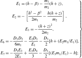 $$\begin{eqnarray}\displaystyle \left.\begin{array}{@{}c@{}}\displaystyle E_{1}=(h-\unicode[STIX]{x1D6FD})-\frac{m_{1}}{m_{2}}(h+z),\\ \displaystyle E_{2}=-\left[\frac{h^{2}-\unicode[STIX]{x1D6FD}^{2}}{2m_{1}}-\frac{h(h+z)}{m_{2}}\right],\\ \displaystyle E_{3}=-\frac{(h+z)^{2}}{2m_{2}},\\ \displaystyle E_{6}=-\frac{D_{1}D_{2}}{6m_{1}}-\frac{E_{2}D_{1}}{E_{1}}-\frac{D_{3}}{2}[h+(E_{2}m_{1}/E_{1})],\\ \displaystyle E_{7}=-\frac{D_{1}E_{3}}{2E_{1}}+\frac{E_{3}D_{4}}{3}-\frac{D_{3}}{2}[(E_{3}m_{1}/E_{1})-h];\end{array}\right\} & & \displaystyle\end{eqnarray}$$
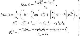 $$\begin{eqnarray}\displaystyle \left.\begin{array}{@{}c@{}}\displaystyle f_{1}(x,t)=\frac{E_{2}p_{1x}^{(0)}+E_{3}p_{2x}^{(0)}}{E_{1}},\\ \displaystyle f_{2}(x,t)=\frac{1}{m_{2}}\left\{\left[h+\frac{E_{2}}{E_{1}}m_{1}\right]p_{1x}^{(0)}+\left[\frac{E_{3}}{E_{1}}m_{1}-h\right]p_{2x}^{(0)}\right\},\\ \displaystyle p_{1x}^{(0)}=p_{2x}^{(0)}+h_{xxx}+\unicode[STIX]{x1D716}_{1}d_{1x}d_{1}-\unicode[STIX]{x1D716}_{2}d_{2x}d_{2},\\ \displaystyle p_{2x}^{(0)}=\frac{-E_{6}(h_{xxx}+\unicode[STIX]{x1D716}_{1}d_{1x}d_{1}-\unicode[STIX]{x1D716}_{2}d_{2x}d_{2})-\tilde{Q}}{E_{6}+E_{7}}.\end{array}\right\} & & \displaystyle\end{eqnarray}$$
Supplementary movies
Supplementary movies are available at https://doi.org/10.1017/jfm.2017.17.