2.1 Setting

Let S be a countable set (alphabet). The one-sided full shift $\Sigma _S$ with set of states S is the set of sequences

$$ \begin{align*}\Sigma_S = \lbrace (x_0x_1 \cdots) \colon x_k \in S \text{ for all } k \in \mathbb{N} \cup \lbrace0\rbrace \rbrace\end{align*} $$

together with the left shift map $\sigma : \Sigma _S \to \Sigma _S$ defined by $(\sigma (x))_k=x_{k+1}$ for all k. We equip $\Sigma _S$ with the product topology induced by the discrete topology on S. This topology is metrizable; one metric is given by $d(x,y)=e^{-t(x,y)}$ , where $t(x,y) := \inf \lbrace k \colon x_k \neq y_k \rbrace $ . The resulting topology is generated by cylinder sets

$$ \begin{align*}[a_0 \cdots a_{n-1}] := \lbrace x \in X \colon x_i = a_i, i = 0, \ldots n-1 \rbrace ~(n \in \mathbb{N}, a_i \in S).\end{align*} $$

With respect to this topology, $\Sigma _S$ is a complete separable metric space, but it is not necessarily compact. A subshift of $\Sigma _S$ , also known as a shift space, is a closed subset $\Sigma $ that is shift invariant ( $\sigma (\Sigma )=\Sigma $ ). A finite word over the alphabet S is a finite sequence of symbols from S. The language of a shift space $\Sigma $ is the set of finite words that appear in some sequence in $\Sigma $ . Such words are called admissible.

Let $A=(t_{ij})_{S \times S}$ be a matrix of zeroes and ones, with columns and rows that are not all zeroes. The TMS with set of states S and transition matrix A is the shift space

$$ \begin{align*}\Sigma := \lbrace (x_0,x_1, \ldots) \in \Sigma_S \colon t_{x_i x_{i+1}}=1 \text{ for all } i \rbrace.\end{align*} $$

Corresponding to this, we can construct a directed graph with set of vertices S and set of edges $\lbrace a \to b \colon t_{ab}=1 \rbrace $ . We can then think of $\Sigma $ as the collection of infinite admissible paths on this directed graph. $\Sigma $ is compact if and only if the S is finite. A subshift of finite type is a compact TMS. Non-compact TMSs are also called countable-state Markov shifts (CMSs).

We assume throughout that $\Sigma $ is topologically mixing, that is, for any two states a and b, there is $N(a,b)$ such that for all $n \geq N(a,b)$ , there is an admissible word of length $n+1$ which starts at a and ends at b.

A function $\phi : \Sigma \to \mathbb {R}$ is called a potential. The modulus of continuity of $\phi $ is captured by the decay of variations of $\phi $ . The variations for $\phi $ are

$$ \begin{align*}\operatorname{\mathrm{var}}_n(\phi)= \sup \lbrace |\phi(x)-\phi(y)| \colon x,y \in \Sigma, x_i = y_i, 0 \leq i \leq n-1\rbrace. \end{align*} $$

A potential $\phi $ is uniformly continuous if and only if $\operatorname {\mathrm {var}}_n(\phi ) \to 0$ . Here, $\phi $ is called the following.

1. (1) $\theta $ -weakly Hölder continuous for some $0<\theta <1$ if there exists a constant $C_\phi> 0$ such that $\operatorname {\mathrm {var}}_n(\phi ) \leq C_{\phi } \theta ^n$ for all $n \geq 2$ . If, in addition, $\operatorname {\mathrm {var}}_1(\phi )$ is finite, $\phi $ is called locally Hölder continuous. Furthermore, if $\phi $ is bounded, then it is called $\theta $ -Hölder, where $\theta $ is called the Hölder exponent of $\phi $ .

2. (2) A function with summable variations if $\sum _{n \geq 2} \operatorname {\mathrm {var}}_n(\phi )< \infty $ .

Note that the condition of being weakly Hölder continuous is stronger than summable variations. None of these two regularity conditions imply boundedness, and it is also possible that $\operatorname {\mathrm {var}}_1(\phi )= \infty $ .

Let $0<\theta <1$ and let $\| \cdot \|_{\theta }$ denote the Hölder norm, which is given by

(2.1) $$ \begin{align} \| \phi \|_{\theta}:= \| \phi \|_{\infty}+ |\phi|_{\theta}, \end{align} $$

where $\| \cdot \|_{\infty }$ is the uniform norm and

(2.2) $$ \begin{align} |\phi |_{\theta}:= \sup \lbrace |\phi(x)- \phi(y)| / \theta^{t(x,y)} \colon x,y \in X, x \neq y\rbrace. \end{align} $$

Let $d_{\theta }$ be the metric coming from the norm $\| \cdot \|_{\theta }$ . Let $A_{\theta }$ be the set of $\theta $ -weakly Hölder continuous strongly positive recurrent potentials with finite Gurevich pressure (see §2.2). Note that it is possible that $d_{\theta }(\phi , \psi )= \infty $ for potentials $\phi $ and $\psi $ in $A_{\theta }$ .

2.2 Thermodynamic formalism for CMS

We use thermodynamic formalism for CMS developed in [Reference Buzzi and Sarig2, Reference Sarig12, Reference Sarig13]. Let $\phi $ be a potential with summable variations. The Birkhoff sums of $\phi $ are denoted by $S_n(\phi ) := \sum _{k=0}^{n-1} \phi \circ \sigma ^k$ . For any state a, let

$$ \begin{align*} \operatorname{\mathrm{Per}}_n(\Sigma,a) &:= \lbrace x \in \Sigma \colon \sigma^n(x)=x, x_0=a \rbrace \quad\text{and }\\ \operatorname{\mathrm{Per}}^*_n(\Sigma,a) &:= \lbrace x \in \operatorname{\mathrm{Per}}_n(\Sigma,a) \colon x_i \neq a \text{ for all } 1 \leq i \leq n-1 \rbrace. \end{align*} $$

We also write

$$ \begin{align*} Z_n(\phi, a) &= \sum_{x \in \operatorname{\mathrm{Per}}_n(\Sigma,a)} e^{S_n\phi(x)}\quad\text{and}\\ Z_n^*(\phi,a) &= \sum_{x \in \operatorname{\mathrm{Per}}^*_n(\Sigma,a)} e^{S_n\phi(x)}. \end{align*} $$

The limit $P_G(\phi ) := \lim _{n \to \infty } {1}/{n} \ln Z_n(\phi ,a)$ exists for all states a and is independent of the choice of state a. Here, $P_G(\phi )$ is called the Gurevich pressure of $\phi $ . When $\phi =0$ , we obtain the Gurevich entropy $h_G(\Sigma )= P_G(0)$ .

It was proved in [Reference Sarig13, Theorem 3] that if , then the Gurevich pressure satisfies a variational principle:

$$ \begin{align*}P_G(\phi)= \sup \bigg\lbrace h_\mu(\sigma)+ \int \phi \,d\mu \bigg\rbrace,\end{align*} $$

where the supremum ranges over all invariant probability measures such that the sum is not of the form $\infty - \infty $ . A measure $\mu _{\phi }$ which attains this supremum is called an equilibrium state for $\phi $ .

2.2.1 Modes of recurrence, RPF operator, and the generalized RPF theorem

Let $P_G(\phi ) < \infty $ and set $\unicode{x3bb} :=e^{P_G(\phi )}$ . Following Sarig, we say that $\phi $ is recurrent if for some state $a, \sum _{n \geq 1} \unicode{x3bb} ^{-n} Z_n(\phi ,a)$ diverges, and is transient if it converges. Further, if $\phi $ is recurrent and $\sum _{n \geq 1}n \unicode{x3bb} ^{-n} Z^*_n(\phi ,a)$ converges, $\phi $ is called positive recurrent. A potential $\phi $ is said to be strongly positive recurrent (SPR) if

(2.3) $$ \begin{align} \limsup_{n \to \infty} \frac{1}{n} \ln Z_n^*(\phi, a) < P_G(\phi). \end{align} $$

(Sarig’s original definition of SPR potentials is given later. Climenhaga [Reference Climenhaga3, §8.5] shows that (2.3) is equivalent.) These definitions can be shown to be independent of the choice of the state a.

For every $\phi $ with summable variations, we associate the RPF operator $L_{\phi }$ which is defined as

$$ \begin{align*}L_\phi(f)(x)= \sum_{\sigma y=x} e^{\phi(y)} f(y).\end{align*} $$

The generalized RPF theorem proved in [Reference Sarig12] relates the modes of recurrence to the eigendata of the RPF operator. We have that $\phi $ is recurrent if and only if there exists a $\unicode{x3bb}>0$ , a positive continuous function $h_{\phi }$ , and a conservative measure $\nu _{\phi }$ which is finite and positive on cylinders such that

$$ \begin{align*}L_{\phi}h_{\phi}=\unicode{x3bb} h_{\phi}\quad\text{and}\quad L_{\phi}^*\nu_{\phi}=\unicode{x3bb} \nu_{\phi}.\end{align*} $$

Here, $\unicode{x3bb} =e^{P_G(\phi )}$ . Additionally, $\phi $ is positive recurrent if and only if $\int h_{\phi } \, d\nu _{\phi } < \infty $ . The measure $dm_{\phi }=h_{\phi }\,d\nu _{\phi }$ is called the RPF measure for $\phi $ . If $\phi $ is positive recurrent and its RPF measure has finite entropy, then it is an equilibrium state for $\phi $ . For subshifts of finite type, this is always the case. Furthermore, if the equilibrium state exists, then it is unique [Reference Buzzi and Sarig2].

We now give Sarig’s original definition of the strong positive recurrence condition in terms of a discriminant. Let $\Sigma $ be a TMS and $a \in S$ . We define an induced system on $[a]$ as $\sigma _a \colon \Sigma _a \to \Sigma _a$ , where $\Sigma _a= \lbrace x \in \Sigma \colon x_0=a, x_i = a \text { infinitely often} \rbrace $ and $\sigma _a= \sigma ^{\tau _a(x)}(x)$ , where $\tau _a(x)= \min \lbrace n \geq 1 \colon x_n=a \rbrace $ .

This system can be given the structure of a TMS as follows. Let $\overline {S}=\lbrace [a, \xi _1, \ldots , \xi _{n-1}, a]: n \geq 1, \xi _i \neq a \rbrace \setminus \emptyset $ . Let $\overline {\Sigma } = \overline {S}^{\mathbb {N} \cup \lbrace 0 \rbrace }$ and $\overline {\sigma }$ be the left shift map on $\overline {\Sigma }$ . Then, $(\overline {\Sigma }, \overline {\sigma })$ is topologically conjugate to $(\Sigma _a, \sigma _a)$ and the conjugacy $\pi : \overline {\Sigma } \to \Sigma _a$ is given by

$$ \begin{align*}\pi([a,\xi_1^0, \ldots \xi_{n_0}^0,a],[a,\xi_1^1, \ldots \xi_{n_1}^1,a],\ldots) := (a,\xi_1^0, \ldots \xi_{n_0}^0,a,\xi_1^1, \ldots \xi_{n_1}^1, a \cdots).\end{align*} $$

Corresponding to every potential function $\phi $ , we get an induced potential $\overline {\phi }: \overline {\Sigma } \to \mathbb {R}$ , which is defined as

$$ \begin{align*}\overline{\phi} := \bigg(\kern-2pt\sum_{i=0}^{\tau_a-1} \phi \circ \sigma^i \bigg) \circ \pi. \end{align*} $$

If $\phi $ is weakly Hölder continuous, then $\overline {\phi }$ is locally Hölder continuous. The a-discriminant of $\phi $ is defined as

$$ \begin{align*}\Delta_a[\phi] := \sup \lbrace P_G(\overline{\phi+p}) \colon p \in \mathbb{R} \text{ such that } P_G(\overline{\phi+p})< \infty \rbrace.\end{align*} $$

A potential $\phi $ is said to be strongly positive recurrent if there exists a state a such that $\Delta _a[\phi ]>0$ . If $\phi $ is strongly positive recurrent, then $P_G(\phi )=0 \iff P_G(\overline {\phi })= 0$ .

2.3 $\overline {d}$ -metric

Ornstein introduced the concept of $\overline {d}$ -distance on the space of invariant measures on a shift space to study the isomorphism problem for Bernoulli shifts. He also proved that the set of processes which are measure theoretically isomorphic to Bernoulli shifts is $\overline {d}$ -closed (see [Reference Ornstein8, Reference Ornstein9]).

Let $(\Sigma ,\sigma )$ be a CMS. We denote the space of Borel probability measures on $\Sigma $ by $\mathscr {M}(\Sigma )$ and let $\mathscr {M}^{\sigma } (\Sigma )$ denote the space of shift invariant Borel probability measures on $\Sigma $ . For $\nu _1$ and $\nu _2$ in $\mathscr {M}^{\sigma } (\Sigma )$ , a joining of $(\Sigma ,\nu _1)$ and $(\Sigma ,\nu _2)$ is a shift invariant measure on $\Sigma \times \Sigma $ with the property that $\mu (A \times \Sigma )= \nu _1(A)$ and $\mu (\Sigma \times B)=\nu _2(B)$ for any measurable subsets A and B of $\Sigma $ . Equivalently, a joining of $(\Sigma ,\nu _1)$ and $(\Sigma ,\nu _2)$ is a shift invariant measure on $\Sigma \times \Sigma $ such that $\pi _1^*\mu =\nu _1$ and $\pi _2^*\mu =\nu _2$ , where $\pi _1, \pi _2$ are projections onto the two coordinates. We now define the $\overline {d}$ -metric in terms of joinings. The following definition is shown to be equivalent to Ornstein’s original definition in [Reference Rudolph11].

Definition 2.1. Let $J(\nu _1,\nu _2)$ be the set of joinings of $(\Sigma ,\nu _1)$ and $(\Sigma ,\nu _2)$ . Let $\delta (x,y)$ be 1 if $x_0 \neq y_0$ and $0$ otherwise. Then,

$$ \begin{align*} \bar{d}(\nu_1,\nu_2) &= \inf_{\mu \in J(\nu_1,\nu_2)} \int \delta(x,y) \, d\mu(x,y) \\ &= \inf_{\mu \in J(\nu_1,\nu_2)} \mu(\lbrace (x,y) \in \Sigma \times \Sigma \colon x_0 \neq y_0 \rbrace). \end{align*} $$

The more familiar topology on the space of Borel probability measures on a metric space Y is the weak* topology. A sequence $\mu _n$ in $\mathscr {M}(Y)$ is said to converge weak* to $\mu $ if $\int f \,d\mu _n \to \int f \,d\mu $ for all bounded continuous function f on Y. When Y is compact, $\mathscr {M}(Y)$ is compact in the weak* topology. When Y is not compact, it is important to first understand under what conditions does a sequence in $\mathscr {M}(Y)$ have a convergent subsequence.

A subset of $\mathscr {M}(Y)$ is said to be tight if for every $\epsilon> 0$ , there exists a compact subset $K_\epsilon $ , such that $\mu (K_{\epsilon }^c)< \epsilon $ for all measures $\mu $ in the subset. If Y is a complete separable metric space and $\mu _n$ is a tight sequence in $\mathscr {M}(Y)$ , then the Helly–Prokhorov theorem gives that it has a subsequence that converges weak* to some $\mu $ in $\mathscr {M}(Y)$ . Hence, every tight subset of $\mathscr {M}(Y)$ is precompact.

Proof. Since every finite Borel measure on a complete separable metric space is tight, then for given $\epsilon> 0$ , we get compact sets A and B in $\Sigma $ such that $\nu _1(\Sigma \setminus A) < \epsilon $ and ${\nu _2(\Sigma \setminus B)<\epsilon }$ .

Let $K=A \times B \subset \Sigma \times \Sigma $ and take m in $J(\nu _1, \nu _2)$ . Since

we conclude that

$$ \begin{align*}m((\Sigma \times \Sigma) \setminus (A \times B)) \leq \nu_1(\Sigma \setminus A) + \nu_2(\Sigma \setminus B) < 2\epsilon. \end{align*} $$

Therefore, $J(\nu _1, \nu _2)$ is tight; hence, it is pre-compact in the weak*-topology. Also, $J(\nu _1, \nu _2)$ is closed. Indeed, let $\mu _n$ be a sequence in $J(\nu _1,\nu _2)$ converging to $\nu $ and consider for $f \in C_b(X)$ ,

$$ \begin{align*}\int f \circ \pi_1 \,d\nu = \lim_{n \to \infty} \int f \circ \pi_1 \,d\mu_n= \lim_{n \to \infty} \int f \, d\nu_1= \int f\, d\nu_1.\end{align*} $$

Hence, $(\pi _1)_*\nu =\nu _1$ and similarly $(\pi _2)_*\nu =\nu _2$ . So, $\nu $ is in $J(\nu _1, \nu _2)$ . Hence, $J(\nu _1, \nu _2)$ is compact.

3.1 Definitions and basic facts

The notion of g-functions and g-measures was introduced to ergodic theory in [Reference Keane6] and is a useful tool in thermodynamic formalism. In [Reference Walters14], Walters gave a proof of Ruelle’s operator theorem using g-measures.

Let $\Sigma $ be a full shift with a countable set of states S and let $\sigma $ be the left shift map on $\Sigma $ . A continuous function $g \colon \Sigma \to (0,1]$ is called a g-function if

$$ \begin{align*}\sum_{y \in \sigma^{-1}(x)} g(y)=1 \quad\text{for all } x \in \Sigma.\end{align*} $$

Conformal measures for g-functions are called g-measures, that is, $\mu $ is a g-measure if and only if $L_g^*(\mu )=\mu $ . For a given g-function, a g-measure is a $\sigma $ -invariant measure $\mu $ in the space of Borel probability measures of $\Sigma $ such that

$$ \begin{align*}g(x)= \lim_{|A| \to 0, x \in A} \frac{\mu(A)}{\mu(\sigma(A))},\quad \mu \text{ -a.e}\end{align*} $$

where $|A|$ denotes the diameter of A and a.e. means almost everywhere.

We denote by $[x]^n= \lbrace y: y_k=x_k$ for all $k \leq n \rbrace $ , the cylinder of those points which agree with x for the first $n+1$ places. The measure $\mu $ is a g-measure if

$$ \begin{align*}\displaystyle\lim_{n \to \infty} \frac{\mu([ix]^{n+1})}{\mu([x]^n)}= g(ix),\quad \mu \text{ -a.e}.\end{align*} $$

We now discuss a probabilistic interpretation of g-functions and g-measures. We can view $g(ix)$ as a Markov transition probability, giving the probability of moving from x to $ix$ and a g-measure is an invariant measure for this Markov process (see [Reference Quas10]). More precisely, let us consider a sequence of random variables $(X_n)_{n \in \mathbb {Z}}$ taking values in the set of states S. Here, $X_n$ are maps from some probability space $\Omega $ to S. Suppose the sequence satisfies

$$ \begin{align*}\mathbb{P}(X_n=i| X_{n-1}=x_1,X_{n-2}=x_2, \ldots)= g(ix).\end{align*} $$

We fix a natural number n and define $\rho _n \colon \Omega \to \Sigma $ by $(\rho _n(\omega ))_i = X_{n-i}(\omega )$ . The probability distribution on $(X_m)_{m \leq n}$ pushes forward to a probability measure on $\Sigma $ , where $\rho _n^*(\mathbb {P}(A))= \mathbb {P}(\rho _n^{-1}(A)))$ . The g-measures correspond to stationary distributions for the random variables.

For SFTs, continuous functions have at least one g-measure associated to them but uniqueness is not guaranteed. In the cases where g is Hölder continuous or the variations of g are summable, the g-measure is known to be unique (proofs can be found in [Reference Keane6, Reference Walters14]).

Let $\phi $ be a recurrent potential and let $\unicode{x3bb} =e^{P_G(\phi )}$ . Let $h_{\phi }$ be given by the generalized RPF theorem. Then, $g_{\phi }:= {e^{\phi }h_{\phi }}/{\unicode{x3bb} h_{\phi } \circ \sigma }$ is a g-function. The RPF measure for $\phi $ is a g-measure for $g_{\phi }$ .

The following lemmas give some results about the RPF operator associated to continuous g-functions.

Proof. Since

$$ \begin{align*}\lvert f(y) \rvert \leq \|f\|_{\text{sup}}\quad\text{for all } y \in \Sigma \quad \text{ and}\end{align*} $$

$$ \begin{align*}\sum_{y \in \sigma^{-1}(x)} g(y)=1\quad\text{for all } x \in \Sigma,\end{align*} $$

then

$$ \begin{align*}\kern-20pt \| L_{\log g}(f) \|_{\text{sup }} = \sup_{x \in \Sigma} \lvert L_{\log g}(f)(x) \rvert = \sup_{x \in \Sigma} \bigg\lvert\! \sum_{y \in \sigma^{-1}(x)} g(y) f(y) \bigg\rvert \leq \|f\|_{\text{sup}}.\\[-47pt] \end{align*} $$

The following result about dual operators on Banach spaces shows that $L_{\log g}^*$ is also continuous.

Lemma 3.2. Let $T:V \to V$ be a bounded linear operator on a Banach space V. Let $T^*: V^* \to V^*$ be the dual of T, defined by

$$ \begin{align*}T^*(f)= f \circ T\end{align*} $$

Then, $T^*$ is continuous with respect to the weak*-topology on $V^*$ .

Proof. Let $(f_{\alpha })_{\alpha }$ be a net in $V^*$ with weak*-limit f, then

$$ \begin{align*} &f_{\alpha}(Tx) \to f(Tx) \quad\text{for all } x \text{ in } V \implies (f_{\alpha} \circ T)(x) \to (f \circ T)(x)\quad \text{ for all } x \text{ in } V \\ &\implies f_{\alpha} \circ T \xrightarrow{\mathrm{weak}*} f \circ T \implies T^*(f_{\alpha}) \xrightarrow{\mathrm{weak}*} T^*(f).\\[-3.1pc] \end{align*} $$

3.2 Proof of Theorem 1.2

Let $\Sigma $ be the full shift with countable alphabet S. We define the following on the space of continuous g-functions:

$$ \begin{align*} V_n(g) &= \sup_{[x]^{n-1}=[y]^{n-1}} |\kern-2pt \log(g(x))-\log(g(y))|, \\ d(h,g) &= \sup_x |\kern-2pt \log(g(x))-\log(h(x))|= \|\kern-2pt \log(g)-\log(h) \|_{\infty}. \end{align*} $$

Note that when $d(h,g)< \infty $ , there exists c in $(0,1]$ such that

(3.1) $$ \begin{align} g(ix) \geq c h(iy) \quad\text{and}\quad h(iy) \geq c g(ix)\quad \text{ for all } i,x,y. \end{align} $$

In the remainder of this section, we give a proof of Theorem 1.2, which extends [Reference Coelho and Quas4, Theorem 1] to the setting of full shifts on countable alphabets.

3.2.1 Transition probabilities

Let $F:S \times \Sigma \times \Sigma \to (0,1)$ be defined by

$$ \begin{align*}F(i,x,y)=\min(g(ix),h(iy)).\end{align*} $$

Let $\Delta : \Sigma \times \Sigma \to [0,1)$ be given by

$$ \begin{align*}\Delta(x,y)=1-\sum_i F(i,x,y). \end{align*} $$

Let $d(g,h)<\infty $ and set

$$ \begin{align*}c(g,h)=\inf_{i,x,y} \bigg( \min\bigg( \frac{g(ix)}{h(iy)}, \frac{h(iy)}{g(ix)} \bigg) \bigg).\end{align*} $$

Then, for all $i,x,y$ ,

$$ \begin{align*} F(i,x,y) \geq c(g,h) g(ix). \end{align*} $$

So, we get that

$$ \begin{align*} \Delta(x,y)=1-\sum_i F(i,x,y) \geq c(g,h) \leq 1- e^{-(V_1(g)+d(h,g))}. \end{align*} $$

Let $\alpha =1-e^{-(V_1(g)+d(h,g))}$ . For $[x]^{k}=[y]^{k}$ ,

(3.2) $$ \begin{align} \Delta(x,y) &\leq 1-e^{-(V_{k+1}(g)+d(h,g))}. \end{align} $$

We define $G:\Sigma \times \Sigma \to (0,1]$ as follows:

(3.3) $$ \begin{align} G(ix,iy) &= F(i,x,y) \quad\text {and} \end{align} $$

(3.4) $$ \begin{align} G(ix,jy) &= \frac{(g(ix)-F(i,x,y))^+(h(jy)-F(j,x,y))^+}{\Delta(x,y)} \end{align} $$

for $i \neq j$ and $a^+=\max (a,0)$ .

Lemma 3.3. For G defined by (3.3) and (3.4), we have that

$$ \begin{align*} &\sum_i G(ix,jy) = h(jy)\quad\text{for all } j \in S \text{ and } x,y \in \Sigma \quad\text{and} \\&\sum_j G(ix,jy) = g(iy)\quad\text{for all } i \in S \text{ and } x,y \in \Sigma. \end{align*} $$

Proof. We fix $x,y$ and partition the set S as follows: $S=S_g \cup S_h \cup S_0$ , where $S_0{\kern-1pt}={\kern-1pt}\lbrace i {\kern-1pt}\in{\kern-1pt} S: g(ix){\kern-1pt}={\kern-1pt}h(iy) \rbrace , S_g{\kern-1pt}={\kern-1pt} \lbrace i \in S: g(ix)>h(iy)\rbrace , S_h=\lbrace i \in S: g(ix)<h(iy) \rbrace $ ;

$$ \begin{align*} \sum_i F(i,x,y) &= \sum_i \min(g(ix),h(iy)) \\&= \sum_{i \in S_h \cup S_0} g(ix) + \sum_{i \in S_g} h(ix) \\&= \sum_{i \in S_h \cup S_0} g(ix) + 1 - \sum_{i \in S_h \cup S_0} h(ix) \\&= \sum_{i \in S_h \cup S_0} [g(ix)-h(iy)] +1. \end{align*} $$

So, we get that

$$ \begin{align*} \Delta(x,y) &= - \sum_{i \in S_h \cup S_0} [g(ix)-h(iy)],\\ \Delta(x,y) &= \sum_{i \in S_h} [h(iy)-g(ix)]\\ &= \sum_{i} [h(iy)-F(i,x,y)]^+. \end{align*} $$

Finally, we get that

$$ \begin{align*} \sum_j G(ix,jy) &= \sum_{j \neq i} \frac{(g(ix)-F(i,x,y))^+(h(jy)-F(j,x,y))^+}{\Delta(x,y)}\\& \quad +F(i,x,y) \\&= (g(ix)-F(i,x,y))^+ + F(i,x,y) \\&= g(ix) - F(i,x,y) +F(i,x,y) \\&=g(ix). \end{align*} $$

Similarly, we have

$$ \begin{align*}\sum_i G(ix,jy)= h(jy).\\[-47pt] \end{align*} $$

Lemma 3.4. Let $\pi _1: \Sigma \times \Sigma \to \Sigma $ be the projection onto the first coordinate, that is, $\pi _1(x,y)=x$ . Then, the following diagram commutes.

Similarly, let $\pi _2: \Sigma \times \Sigma \to \Sigma $ be the projection onto the second coordinate, that is, $\pi _2(x,y)=y$ . Then, for all $m \in \mathscr {M}(\Sigma \times \Sigma )$ ,

$$ \begin{align*}(\pi_2)_*(L_{\log G}^*(m))= L_{\log g}^*((\pi_2)_*(m)).\end{align*} $$

In particular, if m in $\mathscr {M}(\Sigma \times \Sigma )$ satisfies $(\pi _1)_{*}(m)=\nu _g$ and $(\pi _2)_{*}(m)=\nu _h$ , then $(\pi _1)_{*}(L_{\log G}^*m)=\nu _g$ and $(\pi _2)_{*}(L_{\log G}^*m)=\nu _h$ .

Proof. Consider for $m \in \mathscr {M}(\Sigma \times \Sigma )$ and $f \in C_b(\Sigma )$ ,

$$ \begin{align*} \int f \,d((\pi_1)_*(L_{\log G}^*(m))) &= \int L_{\log G} (f \circ \pi_1) \,dm. \end{align*} $$

For $x,y \in \Sigma $ ,

$$ \begin{align*} L_{\log G} (f \circ \pi_1)(x,y) &= \sum_{i,j} G(ix,jy) ((f \circ \pi_1)(ix,jy)) \\ &= \sum_{i,j} G(ix,jy) f(ix) \\ &= \sum_{i} g(ix) f(ix)\quad (\text{by Lemma } 3.3)\\ &= L_{\log g}(f)(x) \\ &= (L_{\log g}(f) \circ \pi_1)(x,y). \end{align*} $$

Hence, we get that

$$ \begin{align*} \int f \,d((\pi_1)_*(L_{\log G}^*(m))) &= \int L_{\log G} (f \circ \pi_1) \,dm \\ &= \int (L_{\log g}(f) \circ \pi_1) \,dm \\ &= \int f \, d(L_{\log g}^* (\pi_1)_* m). \end{align*} $$

Hence, $(\pi _1)_*(L_{\log G}^*(m))= L_{\log g}^*((\pi _1)_*(m))$ .

Similarly, $(\pi _2)_*(L_{\log G}^*(m))= L_{\log g}^*((\pi _2)_*(m))$ . Finally, if m in $\mathscr {M}(\Sigma \times \Sigma )$ satisfies $(\pi _1)_{*}(m)=\nu _g$ , then

$$ \begin{align*}(\pi_1)_{*}(L_{\log G}^*m)=L_{\log g}^*((\pi_1)_*m)=L_{\log g}^*(\nu_g)=\nu_g.\end{align*} $$

Similarly, we get $(\pi _2)_{*}(L_{\log G}^*m)=\nu _h$ .

3.2.2 Joining

We now produce a joining of $\nu _g$ and $\nu _h$ . For notational convenience, let $T:=L_G^*$ . Then, T is an affine map of $\mathscr {M}(\Sigma \times \Sigma )$ . Here, T is weak*-continuous (Lemmas 3.2 and 3.1). Our problem now translates to finding a fixed point for T. We do this by defining a tight sequence of measures.

Let

$$ \begin{align*}P_{\nu_g, \nu_h} = \lbrace m \in \mathscr{M}(\Sigma \times \Sigma) \colon m \text{ has marginals } \nu_g \text{ and } \nu_h \rbrace. \end{align*} $$

Then, take $m_0= \nu _g \times \nu _h \in P_{\nu _g, \nu _h}$ . Define a sequence as

$$ \begin{align*}m_n= \frac{1}{n} \sum_{k=0}^{n-1} T^k(m_0).\end{align*} $$

Then, by Lemma 3.5, for all n, $m_n$ is in $P_{\nu _g, \nu _h}$ .

By Lemma 2.1, there is a convergent subsequence, say $(m_{n_j})_j$ . Let $\mu $ be the weak*-limit of this subsequence. We claim that $T\mu =\mu $ . Then, since $\mu $ is a fixed point for the dual of the RPF operator, we get that $\mu $ is invariant for the map $\sigma \times \sigma $ .

Lemma 3.5. Let $\mu $ be the weak*-limit of a subsequence of the sequence

$$ \begin{align*}m_n= \frac{1}{n} \sum_{k=0}^{n-1} T^k(m_0).\end{align*} $$

Then, $\mu $ is a fixed point for T.

Proof. Let $K \subset \Sigma \times \Sigma $ be compact. Then, the weak*-topology on $M(K)$ , the space of measures on K, is metrizable. One metric that induces the weak*-topology on $M(K)$ is given by the following. Let $(f_n)_n \subset C(K)$ be a dense subset with $\| f_n \|_{\infty } =1$ for all n. We can use this to define a metric $d_K$ by

$$ \begin{align*}d_K(\mu,\nu)= \sum_{n=1}^{\infty}\frac{|\kern-2pt\int_K f_n \, d\mu- \int_K f_n \, d\nu |}{2^n}.\end{align*} $$

This defines a pseudo-metric on $\mathscr {M}(\Sigma \times \Sigma )$ and

$$ \begin{align*}d_K(T\mu,\mu) \leq d_K(T\mu,Tm_{n_j})+d_K(Tm_{n_j},m_{n_j})+d_K(m_{n_j},\mu). \end{align*} $$

Any continuous function f on K can be extended to a continuous function on $\Sigma \times \Sigma $ , as K is compact. Also, $\mu $ is the limit of the subsequence $(m_{n_j})$ in the weak*-topology on $\mathscr {M}(\Sigma \times \Sigma )$ , so we get that $d_K(m_{n_j},\mu ) \to 0$ . Since T is continuous, $d_K(T\mu ,Tm_{n_j}) \to 0$ .

For the middle term, observe the following:

$$ \begin{align*} m_{n_j} &= \frac{1}{n_j} \sum_{k=0}^{n_j-1} T^k(m_0), \\ Tm_{n_j} &= \frac{1}{n_j} \sum_{k=1}^{n_j} T^k(m_0), \\ d_K(Tm_{n_j},m_{n_j}) &= d_K \bigg(\frac{1}{n_j} \sum_{k=0}^{n_j-1} T^k(m_0), \frac{1}{n_j} \sum_{i=1}^{n_j} T^i(m_0) \bigg) \\ &= \sum_{n=1}^{\infty}\frac{|\kern-2pt\int_K f_n \, d( ({1}/{n_j}) \sum_{k=0}^{n_j-1} T^k(m_0) )- \int_K f_n \, d( ({1}/{n_j}) \sum_{i=1}^{n_j} T^i(m_0) ) |}{2^n} \\ &= \sum_{n=1}^{\infty}\frac{({1}/{n_j}) |\kern-2pt\int_K f_n \, d( m_0 )- \int_K f_n \, d( T^{n_j}(m_0) ) |}{2^n} \\ &\leq \sum_{n=1}^{\infty} \frac{1}{2^n n_j} \bigg( \bigg|\kern-2pt\int_K f_n \, d( m_0 ) \bigg| + \bigg|\kern-2pt\int_K f_n \, d( T^{n_j}(m_0) ) \bigg| \bigg) \\ &= \sum_{n=1}^{\infty} \frac{1}{2^n n_j} ( m_0(K) + T^{n_j}(m_0)(K) ) \\ &= \frac{1}{n_j} ( m_0(K) + T^{n_j}(m_0)(K) ) \leq \frac{2}{n_j} \to 0. \end{align*} $$

Hence, $d_K(T\mu ,\mu )=0$ ; therefore, $T\mu |_K=\mu |_K$ . Since the compact subset K was arbitrarily chosen, $T\mu =\mu $ .

3.2.3 Estimating $\overline {d}(\nu _g,\nu _h)$

We want to get an upper bound on $\bar {d}(\nu _g,\nu _h)$ . We do this by estimating $\int \delta (x,y) \, d\mu $ , where

$$ \begin{align*} \delta(x,y)= \begin{cases} 1, & x_0 \neq y_0, \\ 0 & \text{otherwise}. \end{cases} \end{align*} $$

Let $\pi (x,y)= \inf \lbrace n \geq 0: x_n \neq y_n \rbrace $ , then $\delta (x,y)=1$ if and only if $\pi (x,y)=0$ .

Let $(X_n)_{n \in \mathbb {Z}}$ and $(Y_n)_{n \in \mathbb {Z}}$ be stochastic processes taking values in the set of states S. Let $X_{n-}$ denote the sequence $(X_{n-1},X_{n-2} \cdots ) \in \Sigma $ and $Y_{n-}$ be similarly defined. Let the transition probabilities for the pair $(X_n,Y_n)$ be given by

$$ \begin{align*}\mathbb{P}(X_n=i, Y_n=i| X_{n-}=x, Y_{n-}=y) = G(ix,jy),\end{align*} $$

where G is as defined in (3.3) and (3.4).

Define a process $(Z_n)_{n \in \mathbb {Z}}$ taking values in $\mathbb {N} \cup \lbrace 0 \rbrace $ by

$$ \begin{align*}Z_n=\pi(X_{n-},Y_{n-}).\end{align*} $$

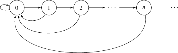
To estimate $\int \delta (x,y) \,d\mu $ , it is sufficient to estimate $\int \chi _{[0]}\,d\mu '$ , where $\mu '$ is the induced measure on the $\mathbb {Z}$ -valued process. For the $\mathbb {Z}$ -valued process, the only valid transitions are from n to $0$ or from n to $n+1$ (see Figure 1).

Figure 1

Valid transitions for the $\mathbb {Z}$ -valued process.

Let $\tau $ be the return time to state $0$ . Since the proportion of time spent by the above process in the state 0 is the reciprocal of the expected return time to state zero, we have that

$$ \begin{align*}\int \delta(x,y) \,d\mu= \int \chi_{[0]}\,d\mu' =\frac{1}{\mathbb{E}(\tau)},\end{align*} $$

where $\mathbb {E}(\tau )$ is the expected return time to state $0$ . Now,

$$ \begin{align*}\mathbb{E}(\tau)=\sum_{k=1}^{\infty} k \mathbb{P}(\tau=k)= \sum_{k=1}^{\infty} \mathbb{P}(\tau \geq k).\end{align*} $$

Consider

$$ \begin{align*} \mathbb{P} [\tau \geq k] &= \frac{1}{\mu(A_0)} \int_{A_0}\sum_{i_1 \cdots i_k} \mathbb{P} ( X_{n+1} \cdots X_{n+k}\\&= Y_{n+1} \cdots Y_{n+k}= i_1 \cdots i_k | X_{n^-} =x, Y_{n^-}=y ) \,d\mu(x,y) \\&= \frac{1}{\mu(A_0)} \int_{A_0} \sum_{i_1 \cdots i_k} F(i_1,x,y) F(i_2,i_1x,i_1y) \cdots\\&\qquad\quad F(i_k , i_{k-1}\cdots i_2i_1x,i_{k-1}\cdots i_2i_1y) \,d\mu(x,y). \end{align*} $$

Now, by (3.2), we get that

$$ \begin{align*}\sum_{i_j} F(i_j , i_{j-1}\cdots i_2i_1x,i_{j-1}\cdots i_2i_1y) \geq e^{-(V_{j+1}(g)+d(g,h))}.\end{align*} $$

We get that

$$ \begin{align*} \mathbb{P} [\tau \geq k ] \geq \prod_{j=1}^{k} (e^{-(V_{j+1}(g)+d(g,h))}). \end{align*} $$

Hence,

(3.5) $$ \begin{align} \mathbb{E}(\tau) \geq \sum_{n=1}^{\infty} \prod_{i=1}^n (e^{-(V_{i+1}(g)+d(h,g))}) = \sum_{n=1}^{\infty}\bigg( \prod_{i=1}^n e^{-V_{i+1}(g)}\bigg) (e^{-d(h,g)})^n. \end{align} $$

This is a power series in $e^{-d(h,g)}$ . As $d(h,g) \to 0$ , $e^{-d(h,g)} \to 1$ . By Abel’s theorem,

$$ \begin{align*}\sum_{n=1}^{\infty} \prod_{i=1}^n (e^{-V_{i+1}(g)}) (e^{-d(h,g)})^n \to \sum_{n=1}^{\infty} \prod_{i=1}^n e^{-V_{i+1}(g)}.\end{align*} $$

Here, $\sum _{n=1}^{\infty } \prod _{i=1}^n e^{-V_{i+1}(g)} = \infty $ is equivalent to the condition (1.1) in the hypothesis, which completes the proof.

We now get Theorem 1.3 as a corollary.

Proof of Theorem 1.3

Let $\sum _{i=1}^{\infty } V_{i+1}(g) \leq L_g<\infty $ . Then, by (3.5), we get that

$$ \begin{align*}\mathbb{E}(\tau) \geq \sum_{n=1}^{\infty} e^{-L_g} (e^{-d(g,h)})^n = e^{-L_g} \frac{e^{-d(g,h)}}{1-e^{-d(g,h)}}= e^{-L_g} (e^{d(g,h)}-1)^{-1}.\end{align*} $$

If $d(g,h) \leq \ln (2)$ , then $e^{d(g,h)}-1 \leq 2d(g,h)$ , we get

(3.6) $$ \begin{align} \overline{d}(\nu_g,\nu_h)\leq \mathbb{E}(\tau)^{-1} \leq e^{L_g}(e^{d(g,h)}- 1) \leq 2e^{L_g}d(g,h). \end{align} $$

In particular, if $\log (g)$ is $\theta $ -weakly Hölder, then $V_k(g) \leq C_g \theta ^k$ for all $k \geq 2$ , then

$$ \begin{align*}\sum_{i=1}^{\infty} V_{i+1}(g) \leq \sum_{i=1}^{\infty} C_g \theta^{i+1} = C_g \frac{\theta^2}{1-\theta}:=L_g.\end{align*} $$

Combining this with (3.6), we get that

$$ \begin{align*}\overline{d}(\nu_g,\nu_h) \leq 2e^{L_g} d(g,h).\end{align*} $$

4.1 Spectral gap property

We begin by first describing the spectral gap property and the Banach space on which the Ruelle operator associated with an SPR potential acts with a spectral gap. Recall that the Ruelle operator associated to potential $\phi $ is defined as

$$ \begin{align*}L_\phi(f)(x)= \sum_{\sigma y=x} e^{\phi(y)} f(y).\end{align*} $$

Let dom $(L_\phi )$ denote the collection of all functions f such that the sum converges for all x in X. For the following terminology and results, see [Reference Cyr and Sarig5]. For the remainder of the discussion, we will let $\phi $ be a $\theta $ -weakly Hölder continuous potential with finite Gurevich pressure.

Strong positive recurrence is a necessary and sufficient condition for the spectral gap property.

Fix $0<\theta <1$ . Let $\phi $ be a $\theta $ -weakly Hölder continuous potential with finite Gurevich pressure that is strongly positive recurrent. We describe a space $\mathscr {B}$ on which $L_\phi $ acts with a spectral gap.

Fix a state a such that $\Delta _a[\phi ]>0$ . Without loss of generality, we can assume that $P_G(\phi )=0$ . We induce on the state as described in §2.2.1. Then, $P_G(\overline {\phi })=0$ . By strong positive recurrence, there exists $\epsilon _a>0$ such that $0<P_G(\overline {\phi +2\epsilon _a})< \infty $ . Also, since $t \to P_G(\overline {\phi +t})$ is continuous, we can choose $\epsilon _a>0$ small enough such that

(4.1) $$ \begin{align} 0<\theta e^p< 1 \quad\text{where } p:=P_G(\overline{\phi+\epsilon_a}). \end{align} $$

Let

(4.2)

Then, $\psi $ is strongly positive recurrent and $P_G(\psi )=0$ . By the generalized RPF theorem, there exists a Borel measure $\nu _0$ which is finite and positive on cylinders, and a positive continuous function $h_0:X \to \mathbb {R}$ , such that

$$ \begin{align*}L_\psi^* \nu_0=\nu_0, ~ L_\psi h_0=h_0 \quad\text{and}\quad \int h_0 \,d\nu_0=1.\end{align*} $$

Moreover, $\operatorname {\mathrm {var}}_1[\log h_0] \leq \sum _{k \geq 2} \operatorname {\mathrm {var}}_k(\phi )$ . Setting $c:= \exp (\sum _{k \geq 2} \operatorname {\mathrm {var}}_k(\phi ))$ , we see that for every x,

(4.3) $$ \begin{align} c^{-1} h_0[x_0] \leq h_0(x) \leq c h_0[x_0],\end{align} $$

where $h_0[x_0] := \sup _{[x_0]} h_0$ .

Define for $x,y \in X$ ,

$$ \begin{align*} t(x,y) &:= \min \lbrace n \colon x_n \neq y_n \rbrace \quad\text{where } \min \emptyset= \infty\quad \text{and}\\ s_a(x,y) &:= \# \lbrace 0 \leq i \leq t(x,y)-1 \colon x_i=y_i=a \rbrace. \end{align*} $$

Let $\mathscr {B}$ be the collection of continuous functions $f:X \to \mathbb {C}$ for which

$$ \begin{align*}\|f\|_{\mathscr{B}}:= \sup_{b \in S} \frac{1}{h_0[b]} \bigg[ \sup_{x \in [b]} |f(x)| +\sup_{x \neq y \in [b]} \bigg\lbrace \frac{|f(x)-f(y)|}{\theta^{s_a(x,y)}} \bigg\rbrace\bigg] < \infty.\end{align*} $$

Here, $L_\phi $ acts with a spectral gap on $(\mathscr {B}, \| \cdot \|_{\mathscr {B}})$ .

4.2 Operator depends continuously on potential

Let $\| \cdot \|_{\theta }$ denote the Hölder norm given by $\| \phi \|_{\theta }:= \| \phi \|_{\infty }+ |\phi |_{\theta }$ , where $\| \cdot \|_{\infty }$ is the uniform norm and $|\phi |_{\theta }:= \sup \lbrace |\phi (x)- \phi (y)| / \theta ^{t(x,y)} \colon x,y \in X, x \neq y\rbrace $ .

Let $\phi $ and $\tau $ be locally $\theta $ -Hölder-continuous strongly positive recurrent potentials with finite Gurevich pressure. Fix a state a such that $\Delta _a[\phi ]>0$ and $\Delta _a[\tau ]>0$ . Without loss of generality, assume that $P_G(\phi )=P_G(\tau )=0$ (otherwise, we pass to $\phi -P_G(\phi )$ and $\tau -P_G(\tau )$ ). Consider

$$ \begin{align*}\|L_{\phi}-L_{\tau} \| = \sup_{\|f\|_{\mathscr{B}}=1} \|L_{\phi}f - L_{\tau}f \|_{\mathscr{B}}. \end{align*} $$

Proof of Lemma 4.2

Let $f \in \mathscr {B}$ with $\| f \|_{\mathscr {B}}=1$ . Now,

(4.4) $$ \begin{align} \|L_{\phi}f - L_{\tau}f \|_{\mathscr{B}} & = \sup_{b \in S} \frac{1}{h_0[b]} ~~ \sup_{x \in [b]} |L_{\phi}f(x)-L_{\tau}f(x)| \nonumber\\ & \quad + \sup_{x,y \in [b], x \neq y} \lbrace |L_{\phi}f(x)-L_{\tau}f(x)-L_{\phi}f(y)+L_{\tau}f(y)|/\theta^{s_a(x,y)} \rbrace. \end{align} $$

Since $h_0$ is an eigenfunction for $L_{\psi }$ , we have that $h_0(x)=\sum _{\sigma (y)=x} e^{\psi (y)}h_0(y)$ , where $\psi $ is as given by (4.2). Furthermore, by the definition of the norm $\| \cdot \|_{\mathscr {L}}$ and (4.3),

(4.5) $$ \begin{align} |f(y)| \leq \|f\|_{\mathscr{B}} h_0[b] \leq c|h_0(y)|. \end{align} $$

By definition, , so

(4.6) $$ \begin{align} \phi \leq \psi+p. \end{align} $$

For $x \in [b]$ , we have the following calculation:

$$ \begin{align*} \bigg| \kern-2pt\sum_{r \to b} e^{\phi(rx)}f(rx) \bigg| &\leq \sum_{r \to b} e^{\phi(rx)} |f(rx)| \nonumber \\ &\leq \sum_{r \to b} e^{\phi(rx)}ch_0(rx) \quad(\text{using } (4.5)) \nonumber \\ & \leq c e^p \sum_{r \to b} e^{\psi(rx)}h_0(rx) \quad(\text{using } (4.6)), \nonumber \end{align*} $$

and hence,

(4.7) $$ \begin{align} \bigg| \kern-2pt\sum_{r \to b} e^{\phi(rx)}f(rx) \bigg| \leq c e^p h_0(x) \quad(\text{using } L_{\psi} h_0 = h_0). \end{align} $$

We begin by considering the first term in (4.4). Let $g=\tau -\phi $ . Fix a state $b \in S$ and consider for $x \in [b]$ ,

(4.8) $$ \begin{align} \bigg| \frac{L_{\phi}f(x)-L_{\tau}f(x)}{h_0(x)} \bigg|&= \bigg| \frac{\sum_{\sigma(y)=x}(e^{\phi(y)}-e^{\tau(y)})f(y)}{h_0(x)} \bigg| \nonumber \\ &= \bigg| \frac{\sum_{\sigma(y)=x}e^{\phi(y)}(1-e^{g(y)})f(y)}{h_0(x)} \bigg| \nonumber \\ &\leq \frac{\sum_{\sigma(y)=x} e^{\phi(y)}|1-e^{g(y)}| |f(y)| }{h_0(x)} \nonumber \\ &\leq (e^{\|\phi-\tau \|_{\infty}}-1 ) \frac{\sum_{\sigma(y)=x} e^{\phi(y)} |f(y)| }{h_0(x)} \nonumber \\ &\leq c (e^{\|\phi-\tau \|_{\infty}}-1 ) e^p \quad(\text{using } (4.7)) \nonumber \\ &\leq c (C\| \phi - \tau \|_{\infty}) e^p \quad(\text{for } \|\phi-\tau\|_{\infty} <1). \end{align} $$

Since $h_0[b] \geq c^{-1} h_0(x)$ for all $x \in [b]$ , we get the following upper bound for the first term in (4.4):

(4.9) $$ \begin{align} \sup_{b \in S} \frac{1}{h_0[b]} ~~ \sup_{x \in [b]} |L_{\phi}f(x)-L_{\tau}f(x)| \leq C \| \phi - \tau \|_{\infty} e^p. \end{align} $$

Now, we consider the second term in (4.4). For $x,y $ in $[b]$ with $x \neq y$ , consider

(4.10) $$ \begin{align} &|L_{\phi}f(x)-L_{\tau}f(x)-L_{\phi}f(y)+L_{\tau}f(y)|/(h_0[b]\theta^{s_a(x,y)}) \nonumber \\ &\quad= \bigg|\frac{\sum_{r \to b} e^{\phi(rx)}f(rx)-e^{\tau(rx)}f(rx)-e^{\phi(ry)}f(ry)+e^{\tau(ry)}f(ry)}{\theta^{s_a(x,y)} h_0[b]} \bigg|. \end{align} $$

We add and subtract $e^{\phi (rx)}f(rx)e^{(\tau -\phi )(ry)}$ from the quantity inside the sum in the numerator, and rewrite it as follows:

$$ \begin{align*} &|e^{\phi(rx)}f(rx)-e^{\tau(rx)}f(rx)-e^{\phi(ry)}f(ry)+e^{\tau(ry)}f(ry)| \\ &\quad= |e^{\phi(rx)}f(rx)(e^{(\tau-\phi)(ry)}-e^{(\tau-\phi)(rx)})+e^{\phi(rx)}f(rx)(1-e^{(\tau-\phi)(ry)})\\&\qquad-e^{\phi(ry)}f(ry)(1-e^{(\tau-\phi)(ry)}) | \\ &\quad= | e^{\phi(rx)}f(rx)(e^{(\tau-\phi)(ry)}-e^{(\tau-\phi)(rx)})-(1-e^{(\tau-\phi)(ry)})(e^{\phi(ry)}f(ry)\\&\qquad-e^{\phi(rx)}f(rx))|. \end{align*} $$

Using this along with $s_a(x,y) \leq t(x,y)$ , we get that

(4.11) $$ \begin{align} |L_{\phi}f(x)-L_{\tau}f(x)-L_{\phi}f(y)+L_{\tau}f(y)|/(h_0[b]\theta^{s_a(x,y)}) \leq A+B, \end{align} $$

where

$$ \begin{align*} A &= \bigg|\frac{\sum_{r \to b} e^{\phi(rx)}f(rx)(e^{(\tau-\phi)(ry)}-e^{(\tau-\phi)(rx)})}{\theta^{t(x,y)} h_0[b]}\bigg|, \\ B &= \bigg|\frac{\sum_{r \to b}(1-e^{(\tau-\phi)(ry)})(e^{\phi(ry)}f(ry)-e^{\phi(rx)}f(rx))}{\theta^{t(x,y)} h_0[b]}\bigg|. \end{align*} $$

We first estimate the first term in (4.11). Note that for $\| \tau -\phi \|_{\infty } \leq 1$ , there exists $C_0$ such that

(4.12) $$ \begin{align} | e^{(\tau-\phi)(ry)}-e^{(\tau-\phi)(rx)} | &\leq C_0 | (\tau-\phi)(ry)-(\tau-\phi)(rx) | \nonumber \\ &\leq C_0 \|\tau-\phi \|_{\theta} \theta^{t(x,y)}. \end{align} $$

Consider

$$ \begin{align*} A & \leq C_0 \|\tau-\phi\|_{\theta} \theta^{t(x,y)} \frac{\sum_{r \to b} e^{\phi(rx)}|f(rx)|}{\theta^{t(x,y)} h_0[b]} \quad(\text{using } (4.12)) \\ & \leq C_1 \|\tau-\phi\|_{\theta} e^p ~~(h_0[b] = \sup_{[b]} h_0 \text{ using } (4.7) ). \end{align*} $$

Next, let us consider the second term in (4.11). We have that

(4.13) $$ \begin{align} B \leq C_2 \|\tau-\phi\|_{\infty} \frac{ \sum_{r \to b} |(e^{\phi(ry)}f(ry)-e^{\phi(rx)}f(rx))|}{\theta^{t(x,y)} h_0[b]}. \end{align} $$

Now,

(4.14) $$ \begin{align} &|e^{\phi(ry)}f(ry)-e^{\phi(rx)}f(rx)|\nonumber\\ &\quad= |e^{\phi(ry)}f(ry)-e^{\phi(rx)}f(ry)+e^{\phi(rx)}f(ry)-e^{\phi(rx)}f(rx) | \nonumber \\ &\quad= | (e^{\phi(ry)}-e^{\phi(rx)})f(ry)+e^{\phi(rx)}(f(ry)-f(rx)) |. \end{align} $$

Since

(4.15) $$ \begin{align} | f(rx)- f(ry) | \leq \| f\|_{\mathscr{B}} h_0[r] \theta^{t(x,y)} \leq h_0[r] \theta^{t(x,y)}, \end{align} $$

we get

(4.16) $$ \begin{align} \sum_{r \to b} |e^{\phi(rx)}(f(ry)-f(rx)) | &\leq \sum_{r \to b} | e^{\phi(rx)} h_0[r] \theta^{t(x,y)} | \quad(\text{using } (4.15)) \nonumber\\&\leq c \sum_{r \to b} e^{\phi(rx)} h_0(rx) \theta^{t(x,y)} \quad(\text{using } (4.3)) \nonumber \\&\leq c \theta^{t(x,y)} e^p \sum_{r \to b} e^{\psi(rx)} h_0(rx) \quad(\text{using } (4.6)) \nonumber \\&\leq c \theta^{t(x,y)} e^p h_0(x) \quad(h_0 = L_{\psi} h_0) \nonumber \\&\leq c \theta^{t(x,y)} e^p h_0[b] \quad(h_0[b] = \sup_{[b]} h_0 ). \end{align} $$

Since $\phi $ is locally Hölder continuous, there exists $C_{\phi }$ such that for all $x,y$ and r, we have $|\phi (rx)-\phi (ry)| \leq C_{\phi }\theta ^{t(x,y)}$ . So,

(4.17) $$ \begin{align} &\bigg| \kern-2pt\sum_{r \to b} (e^{\phi(ry)}-e^{\phi(rx)})f(ry) \bigg|\nonumber\\ &\quad \leq \sum_{r \to b} e^{\phi(ry)} |(1-e^{\phi(rx)-\phi(ry)})| |f(ry)| \nonumber \\ &\quad\leq c e^p \sum_{r \to b} e^{\psi(ry)} |(1-e^{\phi(rx)-\phi(ry)})| h_0(ry) \quad(\text{similar to } (4.7)) \nonumber \\ &\quad\leq C_3 e^p \sum_{r \to b} e^{\psi(ry)} | \phi(rx)-\phi(ry) | h_0(ry) \nonumber \\ &\quad\leq C_3 e^p C_{\phi} \theta^{t(x,y)} h_0(y)\quad (L_{\psi}h_0 = h_0) \nonumber \\ &\quad\leq C_3 e^p C_{\phi} \theta^{t(x,y)} h_0[b]\quad (h_0[b] = \sup_{[b]} h_0 ). \end{align} $$

Combining (4.13), (4.14), (4.16), and (4.17), we get the following estimate on the second term in (4.11):

(4.18) $$ \begin{align} \bigg|\frac{\sum_{r \to b}(1-e^{(\tau-\phi)(ry)})(e^{\phi(ry)}f(ry)-e^{\phi(rx)}f(rx))}{\theta^{t(x,y)} h_0[b]} \bigg| \leq C_2 \|\tau-\phi\|_{\infty} [ c e^p + C_3 C_{\phi} ]. \end{align} $$

Combining (4.4), (4.9), and (4.18), we get

$$ \begin{align*}\|L_{\phi}f - L_{\tau}f \|_{\mathscr{B}} \leq C \| \phi - \tau \|_{\infty} e^p +C_1 \|\tau-\phi\|_{\theta} e^p+ C_2 \|\tau-\phi\|_{\infty} [ c e^p + C_3 C_{\phi} ]. \end{align*} $$

This completes the proof.

4.3 Eigenfunctions depend continuously on potential

Let $\phi $ and $\tau $ be locally $\theta $ -Hölder-continuous strongly positive recurrent potentials with finite Gurevich pressure. We extend the result of this section to weakly Hölder potentials at the beginning of §4.4. Let $h_{\phi }, h_{\tau }$ be positive continuous functions given by the generalized RPF theorem. Then, $L_{\phi }h_{\phi }= h_{\phi }$ and $L_{\tau }h_{\tau }=h_{\tau }$ .

Lemma 4.3. Let $\phi $ be a locally Hölder, SPR potential with finite Gurevich pressure. Given $\alpha>0$ , there exists $\delta>0$ , such that for $\tau \in A_{\theta }$ such that $d_{\theta }(\phi ,\tau ) < \delta $ , we get that

(4.19) $$ \begin{align} \bigg\| \frac{h_{\phi}}{h_{\phi} \circ \sigma} \frac{h_{\tau} \circ \sigma}{h_{\tau}} - 1 \bigg\|_{\infty} < \alpha. \end{align} $$

Note that (4.19) then holds for all scalar multiples of $h_{\phi }$ and $h_{\tau }$ .

Proof of Lemma 4.3

Let $\mathscr {B}$ be the Banach space on which $L_{\phi }$ acts with a spectral gap. According to the theory of analytic perturbations of linear operators, there exists an $\epsilon>0$ such that every $L: \mathscr {B} \to \mathscr {B}$ which satisfies $\| L - L_{\phi } \| < \epsilon $ has a decomposition of the form $L=\unicode{x3bb} (L) P(L)+N(L)$ , where $P(L)$ and $N(L)$ are bounded operators such that $P(L)^2 =P(L), P(L)N(L)=N(L)P(L), \dim (\mathrm{Im} P(L))=1$ , and the spectral radius of $N(L)$ is less than $\unicode{x3bb} (L)$ . Moreover, if $\epsilon> 0$ is small enough, then $L \to P(L), N(L), \unicode{x3bb} (L)$ are analytic on $\lbrace L \colon \|L-L_{\phi } \|< \epsilon \rbrace $ .

By Lemma 4.2, there exists $\delta>0$ , such that for $\|\phi -\rho \|_{\theta } < \delta $ , we get that $\|L_{\phi }-L_{\rho }\| < \epsilon $ , so $L_{\rho }=\unicode{x3bb} _{\rho } P_{\rho }+ N_{\rho }$ , where $\rho \to P_{\rho }$ is continuous.

Let $\gamma>0$ be given, then there exists $\delta>0$ such that for $\|\rho -\phi \|_{\theta }< \delta $ , ${\| P_{\rho }-P_{\phi }\|<{\gamma }/{2}}$ . Let $\tau $ be such that $\|\tau -\phi \|_{\theta }< {\delta }/{2}$ .

By (4.1), $p \to 0$ as $\epsilon _a \to 0$ . Further, by (4.2), $\phi -p \leq \psi \leq \phi +\epsilon _a$ , so if we take $\epsilon _a, p \in (0, {\delta }/{4})$ , we get that $\| \psi - \phi \|_{\infty }< {\delta }/{2}$ . Moreover, , so for all $n \geq 1, \operatorname {\mathrm {var}}_n(\psi -\phi )=0$ . So, $\| \psi - \phi \|_{\theta }< {\delta }/{2}$ . We get that $\| P_{\psi }-P_{\phi }\|<{\gamma }/{2}$ . Further, $\| \psi -\tau \|_{\theta } <\delta $ and $\| P_{\psi }- P_{\tau } \| < \gamma $ .

Normalize so that the corresponding eigenfunctions $h_{\tau } $ and $h_{\phi }$ satisfy $P_{\psi } h_{\phi }= P_{\psi } h_{\tau }= h_0$ . Then,

$$ \begin{align*} \|h_{\phi} \|_{\mathscr{B}} - \|h_0 \|_{\mathscr{B}} \leq \| h_{\phi} - h_0 \|_{\mathscr{B}} &= \| P_{\phi} h_{\phi}-P_{\psi} h_{\phi} \|_{\mathscr{B}} \\ &\leq \| P_{\phi} - P_{\psi} \| \| h_{\phi} \|_{\mathscr{B}} < \gamma \| h_{\phi} \|_{\mathscr{B}} \\ \implies \|h_{\phi} \|_{\mathscr{B}} &\leq \frac{1}{1-\gamma} \|h_0 \|_{\mathscr{B}}. \end{align*} $$

Similarly,

$$ \begin{align*} \|h_{\tau} \|_{\mathscr{B}} \leq \frac{1}{1-\gamma} \|h_0 \|_{\mathscr{B}}.\end{align*} $$

We want to show that $\| ({h_{\phi }}/({h_{\phi } \circ \sigma })) (({h_{\tau } \circ \sigma })/{h_{\tau }})-1 \|_{\infty }$ is small. For $y \in \Sigma $ and for $\gamma \leq \tfrac 12$ , we have that

$$ \begin{align*} \bigg| \bigg(\frac{h_\phi}{h_0} -1 \bigg)(y) \bigg| &= \bigg| \frac{h_{\phi}(y)-h_{0}(y)}{h_0(y)} \bigg| \\ &\leq c \|h_{\phi}-h_0 \|_{\mathscr{B}} \\ &\leq c \gamma \|h_{\phi}\|_{\mathscr{B}} \\ &\leq c \frac{\gamma}{1-\gamma} \|h_0\|_{\mathscr{B}} \\ &\leq 2\gamma c \|h_0\|_{\mathscr{B}}. \end{align*} $$

So,

$$ \begin{align*}h_0(y)(1-2c\gamma \|h_0\|_{\mathscr{B}} ) \leq h_{\phi}(y) \leq h_0(y)(1+2c \gamma \|h_0\|_{\mathscr{B}} ). \end{align*} $$

Similarly,

$$ \begin{align*}h_0(y)(1-2c\gamma \|h_0\|_{\mathscr{B}} ) \leq h_{\tau}(y) \leq h_0(y)(1+2c \gamma \|h_0\|_{\mathscr{B}} ). \end{align*} $$

Given $1>\alpha >0$ , choose $\beta _1>0$ such that $(({1+\beta _1})/({1-\beta _1}))^2=1+\alpha $ and $\beta _2>0$ such that $1-\alpha =(({1-\beta _2})/({1+\beta _2}))^2$ . Now, choose $\gamma \in (0,\tfrac 12 )$ such that $2c\gamma \|h_0\|_{\mathscr {B}}< \min (\beta _1,\beta _2)$ .

Consider

$$ \begin{align*} \frac{h_{\phi}(y)}{h_{\tau}(y)} &\leq \frac{(1+2c \gamma \|h_{0} \|_{\mathscr{B}} )}{(1-2c \gamma \|h_{0} \|_{\mathscr{B}} )} \\ & \leq \frac{1+\beta_1}{1-\beta_1}. \end{align*} $$

Similarly, ${h_{\tau }(y)}/{h_{\phi }(y)} \leq ({1+\beta _1})/({1-\beta _1})$ .

Hence, we get that

$$ \begin{align*}\frac{h_{\phi}(y)}{h_{\phi} \circ \sigma (y)} \frac{h_{\tau} \circ \sigma(y)}{h_{\tau(y)}} \leq \bigg(\frac{1+\beta_1}{1-\beta_1}\bigg)^2 = 1+\alpha.\end{align*} $$

Also,

$$ \begin{align*} \frac{h_{\phi}(y)}{h_{\tau}(y)} &\geq \frac{(1-2c \gamma \|h_{0} \|_{\mathscr{B}} )}{(1+2c \gamma \|h_{0} \|_{\mathscr{B}} )} \\ & \geq \frac{1-\beta_2}{1+\beta_2}. \end{align*} $$

Similarly, ${h_{\tau }(y)}/{h_{\phi }(y)} \geq ({1-\beta _2})/({1+\beta _2})$ .

So, we get that

$$ \begin{align*}\frac{h_{\phi}(y)}{h_{\phi} \circ \sigma (y)} \frac{h_{\tau} \circ \sigma(y)}{h_{\tau(y)}} \geq \bigg(\frac{1-\beta_2}{1+\beta_2}\bigg)^2 = 1-\alpha.\end{align*} $$

Hence, for all y in $\Sigma $ ,

$$ \begin{align*} \bigg| \frac{h_{\phi}(y)}{h_{\phi} \circ \sigma (y)} \frac{h_{\tau} \circ \sigma(y)}{h_{\tau(y)}} - 1 \bigg| \leq \alpha. \end{align*} $$

Therefore,

$$ \begin{align*} \bigg\| \frac{h_{\phi}}{h_{\phi} \circ \sigma} \frac{h_{\tau} \circ \sigma}{h_{\tau}} - 1 \bigg\|_{\infty} < \alpha.\\[-44pt] \end{align*} $$

4.4 Completion of proof

We begin by extending Lemma 4.3 to weakly Hölder potentials. Let $\tilde {S}=S \times S$ and define $\tilde {\pi }: S^{\mathbb {N} \cup \lbrace 0 \rbrace } \to \tilde {S}^{\mathbb {N} \cup \lbrace 0 \rbrace }$ by

$$ \begin{align*}\tilde{\pi}(x_0 x_1 x_2 \cdots)= (x_0,x_1)(x_1,x_2) \cdots \end{align*} $$

Let $\tilde {\Sigma }= \tilde {\pi }(\Sigma )$ . Then, $\tilde {\pi }$ is a topological conjugacy from $(\Sigma , \sigma )$ to $(\tilde {\Sigma }, \sigma )$ . Given a potential $\phi : \Sigma \to \mathbb {R}$ , let $\tilde {\phi }=\phi \circ \tilde {\pi }: \tilde {\Sigma } \to \mathbb {R}$ . If $\tilde {x}, \tilde {y} \in \tilde {\Sigma }$ are such that $\tilde {x_1} \cdots \tilde {x_k}= \tilde {y_1} \cdots \tilde {y_k}$ , $x=\tilde {\pi }(\tilde {x})$ , and $y=\tilde {\pi }(\tilde {y})$ , we get that $x_1 \cdots x_{k+1}= y_1 \cdots y_{k+1}$ . So,

$$ \begin{align*}|\tilde{\phi}(\tilde{x})-\tilde{\phi}(\tilde{y})| = |\phi(x)-\phi(y)| \leq \operatorname{\mathrm{var}}_{k+1}(\phi).\end{align*} $$

Therefore, $\operatorname {\mathrm {var}}_{k}(\tilde {\phi }) \leq \operatorname {\mathrm {var}}_{k+1}(\phi )$ . Thus, if $\phi $ is weakly Hölder continuous, then $\tilde {\phi }$ is locally Hölder continuous. Further, if $L_{\phi }h_{\phi }= \unicode{x3bb} h_{\phi }$ , we get that

$$ \begin{align*} L_{\tilde{\phi}} \tilde{h}(\tilde{x}) &= \sum_{r \to x_0} e^{\tilde{\phi}((r,x_0)\tilde{x})} \tilde{h}((r,x_0)\tilde{x}) \\ &= \sum_{r \to x_0} e^{\phi(rx)} h(rx) =L_{\phi} h(x) \\ &= \unicode{x3bb} h(x) = \unicode{x3bb} \tilde{h}(x). \end{align*} $$

So, the conclusion of Lemma 4.3 holds for $h_{\tilde {\phi }}$ and $h_{\tilde {\tau }}$ if it holds for $h_{\phi }$ and $h_{\tau }$ . Hence, Lemma 4.3 holds for weakly Hölder potentials.

Finally, to complete the proof of Theorem 1.4, consider the g-functions given by $g_{\phi }= {e^{\phi }h_{\phi }}/({ h_{\phi } \circ \sigma })$ and $g_{\tau }= {e^{\tau }h_{\tau }}/({ h_{\tau } \circ \sigma })$ . We have

$$ \begin{align*}\|\kern-2pt \log(g_{\phi})- \log(g_{\tau})\|_{\infty} \leq \|\phi-\tau\|_{\infty} + \bigg\|\kern-2pt \log \bigg( \frac{h_{\phi}}{h_{\phi} \circ \sigma} \frac{h_{\tau} \circ \sigma}{h_{\tau}} \bigg) \bigg\|_{\infty}. \end{align*} $$

It follows from Lemma 4.3 that $\|\kern -2pt \log (g_{\phi })- \log (g_{\tau })\|_{\infty } \to 0$ as $d_{\theta }(\phi ,\tau ) \to 0$ .

Since $\log (g_{\phi })$ and $\log (g_{\tau })$ have summable variations, so $g_{\phi }$ and $g_{\tau }$ satisfy the condition of Theorem 1.2. The RPF measures $m_{\phi }$ and $m_{\tau }$ are g-measures corresponding to $g_{\phi }$ and $g_{\tau }$ . This completes the proof of Theorem 1.1.