





1. Introduction
Linear magnetohydrodynamic (MHD) stability codes are important tools to investigate the stability properties of fusion plasmas which are magnetically confined in tokamak or stellarator devices.
Axisymmetric tokamaks were the favoured fusion devices for many years. However, the axisymmetry is perturbed by the toroidal field ripple and by error fields. The latter result, for example, from imperfections of the magnetic field coils, ferromagnetic inserts, etc. Although these error fields are small, they constrain the operational space of a tokamak. Error fields can deteriorate the confinement, intensify the growth of instabilities, reduce the toroidal rotation, lock modes and cause disruptions. So, they became a main topic in fusion research. So-called saddle coils were installed in many devices to investigate the effects and to reduce the error fields (e.g. Hender et al. Reference Hender1992; La Haye et al. Reference La Haye, Fitzpartrick, Hender, Morris, Scoville and Todd1992; Buttery et al. Reference Buttery1999). Besides, special error field correction coils were integrated in various tokamaks in order to achieve an optimal correction of the error fields (e.g. Barlow et al. Reference Barlow2001; Piron et al. Reference Piron, Kirk, Liu, Cunningham, Carr, Gowland, Katramados and Martin2020). Yet, the use of such coils is not limited to the compensation of error fields. Depending on their number and location, they can be used to probe the plasma stability (Piron et al. Reference Piron2023), to control resistive wall modes (Okabayashi et al. Reference Okabayashi2005) and to mitigate or even suppress edge localised modes (ELMs) (e.g. Evans et al. Reference Evans2004; Liang et al. Reference Liang2007; Suttrop et al. Reference Suttrop2011; Nazikian et al. Reference Nazikian2015).
Nowadays, stellarators are again a subject of focus in nuclear fusion research. Their inherent properties, namely steady-state operation and the absence of disruptions, are especially important requirements for a fusion power plant (Warmer et al. Reference Warmer2024). Ongoing optimisation of the magnetic field geometries leads to major improvements of their confinement properties. There are quasisymmetric and quasiisodynamic devices. Using magnetic coordinates (Boozer coordinates (Boozer Reference Boozer1982)), the magnetic field strength of quasisymmetric stellarators is symmetric in toroidal direction (quasiaxisymmetric (QA) (Nührenberg et al. Reference Nührenberg, Lotz and Gori1994; Henneberg et al. Reference Henneberg, Drevlak, Nührenberg, Beidler, Turkin, Loizu and Helander2019)), in helical direction (quasihelically symmetric (Nührenberg & Zille Reference Nührenberg and Zille1988)) or in poloidal direction (quasipoloidally symmetric (Spong et al. Reference Spong, Hirshman, Lyon, Berry and Strickler2005)). Quasiisodynamic stellarators have no explicit quasisymmetry, but their contours of the magnetic field strength are closed poloidally and the magnetic field is optimised to confine the trapped particles (Goodman et al. Reference Goodman, Camacho Mata, Henneberg, Jorge, Landreman, Plunk, Smith, Mackenbach, Beidler and Helander2023; Lion et al. Reference Lion2025). Figure 1 shows examples of a three-dimensional (3-D) tokamak equilibrium, a QA and a quasiisodynamic stellarator equilibrium. Here, the tokamak equilibrium is 3-D because of an additional two-periodic perturbation field produced by the magnetic perturbation (MP) coils shown in figure 1(a). In the considered case, the phase offset of the upper coil ring relative to the lower ring amounts to
 $\delta \phi =-90^{\textrm {o}}$
. This weak perturbation field (normal component:
 $b_N\approx \pm 8\,\text{mT}$
) leads to a small corrugationFootnote
1
of the flux surfaces. Here, the maximum corrugation of the plasma boundary amounts to
 $\delta _N\approx \pm 0.8\,\text{cm}$
.
(a,b) The AUG-type equilibrium with MP coils. The colours of the plasma boundary mark (a) the normal component of the MP perturbation field and (b) the corrugation caused by the MP field. The colours of the MP coils indicate the antipodal coil currents. (c) Two-periodic QA equilibrium (reproduced with permission from Nucl. Fusion vol. 59, 2019, p. 106008 and EUROfusion; copyright EURATOM 2019) and (d) five-periodic W7-X equilibrium with the colours indicating the magnetic field strength B (reproduced with permission from Nucl. Fusion vol. 60, 2020, p. 106013 and EUROfusion; copyright EURATOM 2020). The colour range in (d) corresponds to 2.1 (dark blue)
 $\leqslant$
B
 $\leqslant$
2.9 T (yellow).

Figure 1. Long description
Panel A: A heat map of a tokamak device with magnetic perturbation coils. The plasma boundary is color-coded to represent the normal component of the magnetic perturbation field, ranging from -8 to 8 millitesla. The coils are color-coded to indicate antipodal coil currents. Panel B: A heat map of the same tokamak device showing the corrugation caused by the magnetic perturbation field. The corrugation values range from -8 to 8 times 10^-3 meters. Panel C: A heat map of a two-periodic quasi-axisymmetric equilibrium tokamak, with colors indicating the magnetic field strength ranging from 4.201 to 6.122 tesla. Panel D: A heat map of a five-periodic Wendelstein 7-X equilibrium tokamak, with colors indicating the magnetic field strength ranging from 2.1 to 2.9 tesla. The heat maps show variations in magnetic field strength and perturbations across different regions of the tokamak devices.
Due to their 3-D geometry, the numerical description of 3-D tokamaks and stellarators is much more complicated than for axisymmetric tokamaks. There exist numerous numerical tools to investigate the linear stability properties of axisymmetric tokamak plasmas, but only few for 3-D tokamak and stellarator plasmas. Linear stability codes can be subdivided into two major groups. The first group makes use of the ideal MHD energy principle. Axisymmetric codes of this group are, for example, PEST (Grimm et al. Reference Grimm, Greene, Johnson and Killeen1976), PEST 2 (Grimm, Dewar & Manickam Reference Grimm, Dewar and Manickam1983), ERATO (Gruber et al. Reference Gruber, Troyon, Berger, Bernard, Rousset, Schreiber, Kerner, Scheider and Roberts1981), GATO (Bernard, Helton & Moore Reference Bernard, Helton and Moore1981), KINX (Degtyarev et al. Reference Degtyarev, Martynov, Medvedev, Troyon, Villard and Gruber1997), MINERVA-DI (Aiba Reference Aiba2016) and ELITE (Wilson et al. Reference Wilson, Snyder, Huysmans and Miller2002), while DCON3D (Glasser Reference Glasser2025), CAS3D (Schwab Reference Schwab1993; Nührenberg Reference Nührenberg2016) and TERPSICORE (Anderson et al. Reference Anderson, Cooper, Gruber, Merazzi and Schwenn1990; Fu et al. Reference Fu, Cooper, Gruber, Schwenn and Anderson1992) are 3-D codes. A mathematical formulation of the weak form of the stability equation with flow was implemented in the CAS3D code in order to describe the perpendicular ExB flow in stellarators (Nührenberg Reference Nührenberg2021), whereas TERPSICHORE provides a treatment of the pressure anisotropy (Moen & Suzuki Reference Moen and Suzuki2023). The second group of codes solves the linearised MHD equations. Examples of those codes are MISHKA-D (Huysmans et al. Reference Huysmans, Sharapov, Mikhailovskii and Kerner2001), MISHKA-F (Chapman et al. Reference Chapman, Sharapov, Huysmans and Mikhailovskii2006), MARS-F (Liu et al. Reference Liu, Bondeson, Fransson, Lennartson and Breitholtz2000), MARS-K (Liu et al. Reference Liu, Chu, Chapman and Hender2008) and CASTOR (Kerner et al. Reference Kerner, Poedts, Goedbloed, Huysmans, Keegan and Schwarz1991; Huysmans, Goedbloed & Kerner Reference Huysmans, Goedbloed and Kerner1993; Kerner et al. Reference Kerner, Goedbloed, Huysmans, Poedts and Schwarz1998). While these codes take several physical effects into account simultaneously, their application is restricted to axisymmetric plasma equilibria. The CarMa code (Portone et al. Reference Portone, Villone, Liu, Albanese and Rubinacci2008) and its extended version CarMa-D (Bonotto et al. Reference Bonotto, Liu, Villone, Pigatto and Bettini2020) result from the coupling of the 3-D eddy current integral formulation of the CARIDDI code (Albanese & Rubinacci Reference Albanese and Rubinacci1988, Reference Albanese and Rubinacci1997) with the two-dimensional (2-D) MARS-F (Liu et al. Reference Liu, Bondeson, Fransson, Lennartson and Breitholtz2000) and MARS-K (Liu et al. Reference Liu, Chu, Chapman and Hender2008) stability code, respectively. They investigate resistive wall modes of axisymmetric equilibria including a detailed description of 3-D conducting structures of finite widthFootnote 2 surrounding the plasma.
The PSL (grey) of AUG with support (yellow) and current (magenta) bridges and MP coils (green) presented in the thin wall approximation.

The CASTOR3D code (Strumberger & Günter Reference Strumberger and Günter2017) makes use of the thin wall approximation (Merkel & Strumberger Reference Merkel and Strumberger2015). Figure 2 shows the plasma facing surfaces of the passive stabilisation loop (PSL) of ASDEX upgrade (AUG) with support and current bridges and the 16 MP coils as used by the CASTOR3D code. Neglecting their finite width, these multiply connected surface structures are represented by triangles which have different conductivities indicated by various colours, while Fourier representations are used for the plasma boundary and simple, smooth, closed wall structures. To our knowledge, CASTOR3D is the only code that includes two fluid and resistive wall effects and can be applied to 2-D (Strumberger et al. Reference Strumberger, Günter, Lackner and Puchmayr2023; Vanovac et al. Reference Vanovac2026) and 3-D equilibria (Strumberger & Günter Reference Strumberger and Günter2019; Strumberger et al. Reference Strumberger and Günter2020; Puchmayr et al. Reference Puchmayr2023; Puchmayr et al. Reference Puchmayr2023, Reference Puchmayr, Dunne, Strumberger, Willensdorfer, Zohm and Hindenlang2024).
The acronym CASTOR3D stands for ‘complex Alfvén spectrum of toroidal plasmas’ with ‘3D’ indicating its ability to handle 3-D equilibria. The 2-D CASTOR code (Kerner et al. Reference Kerner, Goedbloed, Huysmans, Poedts and Schwarz1998) and CASTOR3D have only the name and the weak formulation of the eigenvalue problem in common. The CASTOR3D also uses a Fourier finite-element discretisation in a flux coordinate system, and its ansatz for the test and eigenfunctions is similar to the 2-D CASTOR code. Besides those similarities of the used method, the CASTOR3D code is a completely new code. Its main characteristics are: (i) inclusion of kinetic effects (e.g. diamagnetic effects, viscosity, etc.) in the MHD equations by expressing them in terms of low-order fluid moments (Chang & Callen Reference Chang and Callen1992b ); (ii) weak formulation of the MHD equations in 3-D general flux coordinates; (iii) integration of modified routines of the STARWALL code (Merkel & Strumberger Reference Merkel and Strumberger2015) to compute the vacuum response and to take multiply connected resistive wall and coil structures into account in the vacuum region; (iv) combination of the MHD equations with the vacuum equations to an extended eigenvalue problem which enables the inclusion of plasma inertia and wall resistivity simultaneously; (v) many-valued current potentials (Lüst & Martensen Reference Lüst and Martensen1960) used in the STARWALL part allow a correct treatment of vertical instabilities; (vi) efficient solution of the 3-D non-Hermitian eigenvalue problem by using the parallelised SLEPc Krylov–Schur solver (Roman et al. Reference Roman, Campos, Dalcin, Romero and Tomás2025); (vii) besides growth rates, oscillation frequencies and Fourier spectra of the modes, the CASTOR3D code also yields the mode structures in real space; (viii) the resistive energy functional, which is implemented in the diagnostic part of CASTOR3D, is used to analyse the energetic composition of the eigenfunctions. It provides information on the different energetic drives and stabilising phenomena of the instability (Puchmayr, Dunne & Strumberger Reference Puchmayr, Dunne and Strumberger2022).
The CASTOR3D code was already successfully applied to external kink modes with low toroidal mode numbers in a QA stellarator configuration including parallel viscosity and toroidal flow (Strumberger & Günter Reference Strumberger and Günter2019), and to resistive internal kink and double tearing modes (DTMs) in Wendelstein 7-X (W7-X) (Strumberger et al. Reference Strumberger and Günter2020). Diamagnetic drift effects were studied for ideal and resistive internal kink modes using simple axisymmetric and 3-D test equilibria (Strumberger et al. Reference Strumberger, Günter, Lackner and Puchmayr2023), and CASTOR3D was also used for benchmarks with nonlinear extended MHD codes (e.g. JOREK (Pamela et al. Reference Pamela, Bhole, Huijsmans, Nkonga, Hoelzl, Krebs and Strumberger2020; Nikulsin et al. Reference Nikulsin, Ramasamy, Hoelzl, Hindenlang, Strumberger, Lackner and Günter2022; Ramasamy et al. Reference Ramasamy, Aleynikova, Nikulsin, Hindenlang, Holod, Strumberger and Hoelzl2024) and NIMSTELL (Patil & Sovinec Reference Patil and Sovinec2024)). While former 3-D CASTOR3D stability calculations were restricted to low toroidal mode numbers, now stability studies are also possible for peeling–ballooning modes in 3-D tokamak (Puchmayr et al. Reference Puchmayr2023, Reference Puchmayr, Dunne, Strumberger, Willensdorfer, Zohm and Hindenlang2024) and stellarator configurations (Strumberger, Puchmayr & Hindenlang Reference Strumberger, Puchmayr and Hindenlang2025) because of increasing memory and computing power, substantial improvement of the performance of the CASTOR3D code (Puchmayr Reference Puchmayr2023) and, last but not least, using high fidelity equilibrium solutions computed with the GVEC code (Hindenlang et al. Reference Hindenlang, Babin, Maj, Ribeiro, Koeberl, Muir, Plunk and Sonnendrücker2025a ).
The article is organised as follows. The underlying theoretical basis of the CASTOR3D code is described in § 2. The first part (§ 2.1) concerns the plasma, that is, the extended MHD equations, their linearisation and weak formulation and the boundary conditions. The second part (§ 2.2) deals with the vacuum energy functional, the vacuum equations and the conducting structures surrounding the plasma, whereas the various types of eigenvalue problems solved by CASTOR3D are subject of § 2.3. The structure and details of the CASTOR3D code are described in § 3. Section 4 gives an overview of stability studies performed with the CASTOR3D and interesting results concerning internal kink and interchange modes (§ 4.1), double tearing and internal resistive kink modes (§ 4.2), locked modes (§ 4.3), edge localised and external modes (§ 4.4), overstable modes (§ 4.5), resistive wall modes (§ 4.6) and vertical instabilities (§ 4.7). A short summary and an outlook to further extensions and applications of the code are given in § 5. Finally, the appendices contain details of the weak formulation (Appendix A) and a short description of the COTRANS code (Appendix B). The latter provides the Fourier representation of equilibrium quantities as needed by the CASTOR3D code.
2. Theory
Resistive wall structures surrounding the plasma complicate the solution of the eigenvalue problem because the vacuum response depends on the eigenvalue. Often, resistive wall mode codes (e.g. CarMa (Portone et al. Reference Portone, Villone, Liu, Albanese and Rubinacci2008) and STARWALL (Merkel & Strumberger Reference Merkel and Strumberger2015)) avoid this problem by using the so-called massless approximation, that is, neglecting the plasma inertia. Using the control surface concept, the CarMa code is a combination of the linear MHD solver MARS-F (Liu et al. Reference Liu, Bondeson, Fransson, Lennartson and Breitholtz2000) and the 3-D CARIDDI code (Albanese & Rubinacci Reference Albanese and Rubinacci1988, Reference Albanese and Rubinacci1997). Neglecting plasma mass and rotation, it couples self-consistently the computation of the eddy currents in the 3-D wall structures to the solution of simplified, single-fluid, ideal and linearised MHD equations for axisymmetric plasma configurations. To treat resistive wall mode problems in the case of 3-D plasma configurations and in the presence of 3-D resistive conducting structures, the STARWALL code uses the thin wall approximation. It takes the potential energy matrix of the plasma provided by the ideal CAS3D codeFootnote 3 (Nührenberg Reference Nührenberg1996) and makes use of a Lagrangian which describes the magnetic energy of the currents in the plasma boundary and in the external wall and coil structures. Applying a variational procedure (Haney & Freidberg Reference Haney and Freidberg1989), an eigenvalue problem was derived which yields the growth rates of slow resistive wall modes. However, the growth rates of realistic plasma configurations are not necessarily slow enough to justify the negligence of the plasma inertia. The plasma may have a finite velocity, and resistivity and/or drift effects may be important. Therefore, Bonotto et al. (Reference Bonotto, Liu, Villone, Pigatto and Bettini2020) improved the CarMa code, called CarMa-D, taking into account plasma dynamics, toroidal rotation and drift-kinetic damping. Concerning the CASTOR3D code, we coupled the linearised MHD equations including resistivity, flow and drift effects with the vacuum equations used in the STARWALL code to an extended eigenvalue problem which correctly accounts for the plasma inertia. It comprises the MHD equations and the equations derived from the vacuum energy functional. In the first part of this section, we will discuss the plasma part of the eigenvalue problem.
2.1. Plasma part
2.1.1. Extended MHD equations
The 2-D CASTOR code is based upon the resistive single-fluid MHD equations (Kerner et al. Reference Kerner, Goedbloed, Huysmans, Poedts and Schwarz1998). We extended these equations step by step including the viscous force density
 $-{ \boldsymbol{\nabla }} \boldsymbol{\cdot }\boldsymbol{\varPi }$
, the heat flux term
 $(\varGamma -1)({m_i}/{\rho }) \boldsymbol{\nabla } \boldsymbol{\cdot }\boldsymbol{q}$
, the electron pressure term
 $({\alpha }/{\rho }) {\boldsymbol{\nabla }} p_e$
and the Hall term
 $({\alpha }/{\rho }) \boldsymbol{j} \times {\boldsymbol B}$
. The extended MHD equations read (Schnack et al. Reference Schnack, Barnes, Brennan, Hegna, Held, Kim, Kruger, Pankin and Sovinec2006)
 \begin{align} \frac {\partial \rho }{\partial t} = -\boldsymbol{V} \boldsymbol{\cdot }\boldsymbol{\nabla }\rho - \rho \boldsymbol{\nabla } \boldsymbol{\cdot }{\boldsymbol V}, \end{align}
 \begin{align} \rho \frac {\partial {\boldsymbol V}}{\partial t} = -\rho ({\boldsymbol V} \boldsymbol{\cdot }{ \boldsymbol{\nabla }}) {\boldsymbol V} -{\boldsymbol{\nabla }} p - {\boldsymbol{\nabla }} \boldsymbol{\cdot }\boldsymbol{\varPi } + {\boldsymbol j} \times {\boldsymbol B}, \end{align}
 \begin{align} \frac {\partial T}{\partial t} = -{\boldsymbol V} \boldsymbol{\cdot }{\boldsymbol{\nabla }} T -(\varGamma -1) T {\boldsymbol{\nabla }} \boldsymbol{\cdot }{\boldsymbol V} - (\varGamma -1) \frac {m_i}{\rho } \boldsymbol{\nabla } \boldsymbol{\cdot }{\boldsymbol q}, \end{align}
 \begin{align} {\boldsymbol E} = -{\boldsymbol V} \times {\boldsymbol B} -\frac {\alpha }{\rho } {\boldsymbol{\nabla }} p_e + \frac {\alpha }{\rho } {\boldsymbol j} \times {\boldsymbol B}+\eta {\boldsymbol j} \end{align}
with
 $\alpha$
=
 $\alpha _{\mathrm{s}}( {m_i}/{e})$
, ion mass
 $m_i$
, elementary charge
 $e$
and scaling parameter
 $\alpha _{\mathrm{s}}$
.Footnote
4
These equations are derived from the two-fluid MHD equations (Braginskii Reference Braginskii1965) making several assumptions and approximations, e.g. assuming quasineutrality
 $n=n_i=n_e$
(
 $n_i$
= ion density,
 $n_e$
= electron density), neglecting the electron mass
 $m_e$
(
 $m_i \gg m_e$
, mass density
 $\rho = m_i n + m_e n \approx m_i n$
), using the pressure
 $p=p_i+p_e=n(T_i+T_e)=nT$
(
 $T_i$
= ion temperature,
 $T_e$
= electron temperature,
 $T=T_i+T_e$
) and making the velocity approximation
 $\boldsymbol{V}=(({m_i \boldsymbol{V}_i + m_e \boldsymbol{V}_e})/({m_i+m_e})\approx \boldsymbol{V}_i)$
with
 $\boldsymbol{V}_i$
being the ion velocity. The set of equations is closed with the Maxwell equations
 \begin{align} { \boldsymbol{\nabla }} \boldsymbol{\cdot }{\boldsymbol E} = 0,\,\,\,\,\, {\boldsymbol {\nabla }} \times {\boldsymbol E} = -\frac {\partial {\boldsymbol B}}{\partial t},\,\,\,\,\, { \boldsymbol{\nabla }} \times {\boldsymbol B} = \mu _0 {\boldsymbol j},\,\,\,\,\,{\boldsymbol{\nabla }} \boldsymbol{\cdot }{\boldsymbol B}=0 \end{align}
(
 $\boldsymbol E$
= electric field,
 $\boldsymbol B$
= magnetic field,
 $\boldsymbol j$
= current density). Here, the displacement current
 $\mu _0 \epsilon _0 ({\partial {\boldsymbol E}}/{\partial t})$
is neglected.
In CASTOR3D, the ion velocity
 \begin{align} {\boldsymbol V}_i = \underbrace {\frac {{\boldsymbol E} \times {\boldsymbol B}}{B^2}}_{={\boldsymbol V}_{E\textrm {x}B}} + \underbrace {\frac {\alpha }{\rho } \frac {{\boldsymbol B} \times {\boldsymbol{\nabla }} p_{i}}{B^2}}_{={\boldsymbol V}_i^*} + {\boldsymbol V}^{ext} \end{align}
is implemented with ExB-velocity
 ${\boldsymbol V}_{Ex B}$
, ion diamagnetic drift velocity
 ${\boldsymbol V}_i^*$
and an externally driven velocity
 ${\boldsymbol V}^{ext}$
. Drives of the latter are, for example, neutral beam injection, ion cyclotron range of frequencies waves, etc. (Rice Reference Rice2016).
The viscous stress tensor
 $\boldsymbol{\varPi}$
splits into
 $\boldsymbol\varPi =\boldsymbol\varPi _{\|}+\boldsymbol\varPi _{\wedge }+\boldsymbol\varPi _{\perp }$
with parallel
 $\boldsymbol{\varPi }_{\|}$
, cross (gyroviscous)
 $\boldsymbol{\varPi }_{\wedge }$
and perpendicular
 $\boldsymbol{\varPi }_{\perp }$
parts. The parallel viscous force density is approximated by
 \begin{align} -{\boldsymbol{\nabla }} \boldsymbol{\cdot }\boldsymbol{\varPi }_{\|}\approx \mu _{\|} \Delta _{\|} {\boldsymbol V} \end{align}
with
 $\mu _{\|}$
being the dynamic viscosity coefficient. We neglect the perpendicular viscous force density
 $-\boldsymbol{\nabla } \boldsymbol{\cdot }\boldsymbol{\varPi }_{\perp }$
and use
 \begin{align} - \boldsymbol{\nabla } \boldsymbol{\cdot }\boldsymbol{\varPi }_{\wedge }\approx \rho ({\boldsymbol V}^*_i \boldsymbol{\cdot }{ \boldsymbol{\nabla }}) {\boldsymbol V} \end{align}
for the gyroviscous force density (Chang & Callen Reference Chang and Callen1992a ). This expression is generally known as gyroviscous cancellation. Using (2.7) and (2.8), the momentum equation (2.2) reads
 \begin{align} \rho \frac {\partial {\boldsymbol V}}{\partial t} =- \rho (({\boldsymbol V} - {\boldsymbol V}_i^*) \boldsymbol{\cdot }{\boldsymbol{\nabla }}) {\boldsymbol V} - {\boldsymbol{\nabla }} p + \mu _{\|} {\boldsymbol{\nabla} }_{\|} {\boldsymbol V} + {\boldsymbol j} \times {\boldsymbol B}. \end{align}
Presently, only the parallel part (Braginskii Reference Braginskii1965)
 \begin{align} \boldsymbol{q}_{\|} = \boldsymbol{q}_{\|e}+\boldsymbol{q}_{\|i}= -\kappa _{\|e} \boldsymbol{\nabla} _{\|} T_e -\kappa _{\|i}\boldsymbol{\nabla} _{\|}T_i \end{align}
of the heat flux
 $\boldsymbol q={\boldsymbol q}_{\|}+{\boldsymbol q}_{\wedge }+{\boldsymbol q}_{\perp }$
is included in the energy equation (2.3) with
 $\kappa _{\|e}$
and
 $\kappa _{\|i}$
being the electron and ion thermal conductivity coefficients and
 ${\boldsymbol{\nabla} }_{\|} =({1}/{B^2}){\boldsymbol B} ({\boldsymbol B} \boldsymbol{\cdot }{\boldsymbol{\nabla }} )$
. Besides,
 $\varGamma =5/3$
is used as adiabatic index,
 $\eta$
denotes the plasma resistivity and
 $\mu _0$
is the vacuum permeability.
The extended Ohm’s law (2.4) is simplified by using the drift approximation of the Hall term (Schnack et al. Reference Schnack, Barnes, Brennan, Hegna, Held, Kim, Kruger, Pankin and Sovinec2006)
 \begin{align} {\boldsymbol{\nabla} }_{\perp } p \approx {\boldsymbol j} \times {\boldsymbol B} \end{align}
which leads to
 \begin{align} {\boldsymbol E} = -{\boldsymbol V} \times {\boldsymbol B} - \frac {\alpha }{\rho } { \boldsymbol{\nabla} }_{\|}p_e +\frac {\alpha }{\rho }{\boldsymbol{\nabla} }_{\perp }p_i+ \eta {\boldsymbol j}. \end{align}
Single-fluid codes which include two-fluid effects often use the assumption
 $p_i=p_e=0.5p$
, that is,
 $T_i=T_e$
. Since measured ion and electron temperatures may be different, we use
 \begin{align} p_i=\alpha _T p =n\alpha _T T\,\,\,\,\,\textrm {and}\,\,\,\,\,\,p_e=(1-\alpha _T)p=n(1-\alpha _T) T \end{align}
with
 $0\leqslant \alpha _T \leqslant 1$
. The parameter
 $\alpha _T$
provides an additional degree of freedom that allows to choose a more realistic ratio of ion and electron pressures with respect to the measured temperatures, so that a more realistic treatment of the ion and electron diamagnetic drift effects and the heat flux is possible. Application of the relations (2.13) to the ion drift velocity (2.6), the heat flux (2.10) and the pressure terms of Ohm’s law (2.12) yields
 \begin{align} {\boldsymbol V}_i^* = \frac {\alpha \alpha _T }{\rho } \frac {{\boldsymbol B} \times { \boldsymbol{\nabla }} p} {B^2}, \end{align}
 \begin{align} \boldsymbol{q}_{\|}=-(\kappa _{\|e}(1-\alpha _T)+\kappa _{\|i}\alpha _T)\boldsymbol{\nabla} _{\|}T \end{align}
and
 \begin{align} {\boldsymbol E} = -{\boldsymbol V} \times {\boldsymbol B} - \frac {\alpha }{\rho }{\boldsymbol{\nabla} }_{\|}p +\frac {\alpha \alpha _T}{\rho }{ \boldsymbol{\nabla }} p + \eta {\boldsymbol j}. \end{align}
2.1.2. Linearised extended MHD equations
We use
 $\boldsymbol B=\boldsymbol{\nabla }\times \boldsymbol A$
(
 $\boldsymbol A$
= magnetic vector potential) to fulfil
 $\boldsymbol{\nabla } \boldsymbol{\cdot }\boldsymbol B=0$
, and the Weyl gauge (electric scalar potential
 $\varPhi _E =0$
) yields
 $\boldsymbol E = - ( {\partial \boldsymbol A}/{\partial t})$
. The time dependence of the perturbed quantities is assumed to be
 $\sim \text{e}^{\lambda t}$
with eigenvalue
 \begin{align} \lambda =\gamma + \text{i}\omega . \end{align}
Here,
 $\gamma$
is the growth rate and
 $\omega$
the oscillation frequency of the mode. Using the ansatz
 $f({\boldsymbol r},t)=f_0({\boldsymbol r})+ \text{e}^{\lambda t}f_1({\boldsymbol r})$
for
 $\rho ,\boldsymbol{V},T$
and
 $\boldsymbol A$
, the linearised forms of the extended fluid equations (2.1, 2.9, 2.3, 2.16) read
 \begin{align} \lambda \rho _1 = -{\boldsymbol V}_0 \boldsymbol{\cdot }{\boldsymbol{\nabla }} \rho _1- {\boldsymbol V}_1 \boldsymbol{\cdot }{ \boldsymbol{\nabla }} \rho _0 -\rho _1 {\boldsymbol{\nabla }} \boldsymbol{\cdot }{\boldsymbol V}_0 - \rho _0 {\boldsymbol{\nabla }} \boldsymbol{\cdot }{\boldsymbol V}_1, \end{align}
 \begin{align} \rho _0 \lambda {\boldsymbol V}_1 &= - \rho _1({\boldsymbol V}_0 \boldsymbol{\cdot }{\boldsymbol{\nabla }}) {\boldsymbol V}_0 - \rho _0({\boldsymbol V}_1 \boldsymbol{\cdot }{ \boldsymbol{\nabla }}) {\boldsymbol V}_0 - \rho _0({\boldsymbol V}_0 \boldsymbol{\cdot }{ \boldsymbol{\nabla }}) {\boldsymbol V}_1 \nonumber \\[3.7pt] &\quad + \rho _1({\boldsymbol V}_{i0}^* \boldsymbol{\cdot }{ \boldsymbol{\nabla }}) {\boldsymbol V}_0 + \rho _0({\boldsymbol V}_{i1}^* \boldsymbol{\cdot }{\boldsymbol{\nabla }}) {\boldsymbol V}_0 + \rho _0({\boldsymbol V}_{i0}^* \boldsymbol{\cdot }{\boldsymbol{\nabla }}) {\boldsymbol V}_1 \nonumber \\[3.7pt] &\quad - \frac {1}{m_i}{ \boldsymbol{\nabla }}(\rho _0 T_1) - \frac {1}{m_i}{ \boldsymbol{\nabla }}(T_0 \rho _1) +\mu _{||} \Delta _{||} {\boldsymbol V}_1 \nonumber \\[3.7pt] &\quad + \frac {1}{\mu _0} ({\boldsymbol{\nabla }} \times ({ \boldsymbol{\nabla }} \times {\boldsymbol A}_1) ) \times ({\boldsymbol{\nabla }} \times {\boldsymbol A}_0) \nonumber \\[3.7pt] &\quad + \frac {1}{\mu _0} ({\boldsymbol{\nabla }} \times ({\boldsymbol{\nabla }} \times {\boldsymbol A}_0) ) \times ({\boldsymbol{\nabla }} \times {\boldsymbol A}_1), \end{align}
 \begin{align} \lambda T_1 &= - {\boldsymbol V}_1 \boldsymbol{\cdot }{\boldsymbol{\nabla }} T_0 - {\boldsymbol V}_0 \boldsymbol{\cdot }{\boldsymbol{\nabla }} T_1 -(\varGamma -1) T_1 {\boldsymbol{\nabla }} \boldsymbol{\cdot }{\boldsymbol V}_0 \nonumber \\[3.5pt] &\quad -(\varGamma -1) T_0 { \boldsymbol{\nabla }} \boldsymbol{\cdot }{\boldsymbol V}_1 -(\varGamma -1)\frac {m_i}{\rho _0}\boldsymbol{\nabla }\boldsymbol{\cdot }{\boldsymbol q}_{\|1}, \end{align}
 \begin{align} \lambda \boldsymbol A_1 &= {\boldsymbol V}_1 \times {\boldsymbol B}_0 + {\boldsymbol V_0} \times ({\boldsymbol{\nabla }} \times {\boldsymbol A}_1) +\frac {\alpha }{\rho _0}\frac {1}{B^2_0} {\boldsymbol B}_0 \bigg(({\boldsymbol{\nabla }} \times {\boldsymbol A}_1) \boldsymbol{\cdot }\frac {1}{m_i} {\boldsymbol{\nabla }} (\rho _0 T_0)\bigg) \nonumber \\[3.5pt] &\quad +\frac {\alpha }{\rho _0}\frac {1}{B^2_0} {\boldsymbol B}_0 \bigg({\boldsymbol B}_0 \boldsymbol{\cdot }\frac {1}{m_i} {\boldsymbol{\nabla }}(\rho _1 T_0 + \rho _0 T_1)\bigg) -\alpha \alpha _T \frac {1}{\rho _0}\frac {1}{m_i} { \boldsymbol{\nabla }}(\rho _1 T_0 +\rho _0 T_1) \nonumber \\[3.5pt] &\quad + \alpha \alpha _T \frac {\rho _1}{\rho _0^2} \frac {1}{m_i} {\boldsymbol{\nabla }}(\rho _0 T_0) -\frac {\eta }{\mu _0} ({ \boldsymbol{\nabla }} \times ({ \boldsymbol{\nabla }} \times {\boldsymbol A}_1)). \end{align}
Cylindrical (
 $R,\varphi ,Z$
) and magnetic flux coordinates (
 $s,v,u$
). The flux surfaces described by
 $s= \text{const.}$
lines are shown for a toroidal cross-section of a tokamak plasma.

Here,
 $\rho _0,{\boldsymbol V}_0, T_0,{\boldsymbol A}_0$
are the equilibrium quantities of density, ion velocity, temperature (
 $T_0=T_{0e}+T_{0i}$
) and magnetic vector potential, while
 $\rho _1,{\boldsymbol V}_1, T_1, {\boldsymbol A}_1$
are their perturbations. The perturbation of the ion diamagnetic drift velocity (2.14) and the parallel heat flux term
 $\boldsymbol{\nabla }\boldsymbol{\cdot }{\boldsymbol q}_{\|}$
read
 \begin{align} {\boldsymbol V}_{i1}^*&=-\alpha \alpha _T \frac {\rho _1}{\rho _0^2}\frac {{\boldsymbol B}_0 \times {\boldsymbol{\nabla }} p_0}{B_0^2}+\alpha \alpha _T \frac {1}{\rho _0} \frac {{\boldsymbol B}_0 \times (T_0 { \boldsymbol{\nabla }} \rho _1 + T_1 {\boldsymbol{\nabla }} \rho _0 +\rho _0 {\boldsymbol{\nabla }} T_1 +\rho _1 { \boldsymbol{\nabla }} T_0)}{B_0^2} \nonumber \\[5pt] &\quad +\alpha \alpha _T\frac {1}{\rho _0} \frac {({\boldsymbol{\nabla }} \times {\boldsymbol A_1}) \times {\boldsymbol{\nabla }} p_0}{B_0^2} -2\alpha \alpha _T\frac {1}{\rho _0} \frac {{\boldsymbol B}_0 \boldsymbol{\cdot }({ \boldsymbol{\nabla }} \times {\boldsymbol A_1})}{B_0^4}({\boldsymbol B}_0 \times { \boldsymbol{\nabla }} p_0) \end{align}
and
 \begin{align} \boldsymbol{\nabla }\boldsymbol{\cdot }\boldsymbol{q}_{\|1}&=-(\kappa _{\|e}(1-\alpha _T) +\kappa _{\|i}\alpha _T)\boldsymbol{\cdot }\nonumber \\[5pt] &\quad \left [(\boldsymbol{B}_0\boldsymbol{\cdot }\boldsymbol{\nabla }) \frac {((\boldsymbol{\nabla }\times \boldsymbol{A}_1)\boldsymbol{\cdot } \boldsymbol{\nabla })T_0}{B_0^2} + \boldsymbol{\nabla }\boldsymbol{\cdot }\frac {\boldsymbol{B}_0 (\boldsymbol{B}_0\boldsymbol{\cdot }\boldsymbol{\nabla })T_1} {B_0^2}\right ]. \end{align}
2.1.3. Weak formulation of the MHD equations
The accuracy and the numerical effort of the solution of the linearised MHD equations (2.18–2.21) depends strongly on the chosen coordinates. Since the behaviour of the plasma is extremely anisotropic with respect to the parallel and the perpendicular direction to the magnetic field
 $\boldsymbol{B}_0$
, magnetic flux coordinates are the preferential choice. Figure 3 shows flux surfaces of a tokamak plasma at a toroidal cross-section
 $\varphi = \text{const.}$
and the directions of right-handed cylindrical (
 $R,\varphi ,Z$
) and magnetic flux coordinates (
 $s,v,u$
). The toroidal
 $v$
- and poloidal
 $u$
-coordinates are angle-like variables with
 $0 \leqslant v \lt 1$
and
 $0 \leqslant u \lt 1$
. Coordinate surfaces with constant radial coordinate
 $s$
correspond to flux surfaces with
 $s=0$
being the magnetic axis and
 $s=1$
representing the plasma boundary. Using the right-handed magnetic flux coordinates and the so-called weak formulation, an eigenvalue problem is derived from the linearised MHD equations. For this purpose, we use a procedure analogous to the one described in Huysmans et al. (Reference Huysmans, Goedbloed and Kerner1993) and Kerner et al. (Reference Kerner, Goedbloed, Huysmans, Poedts and Schwarz1998).
In a first step, a complex ansatz is made for the perturbed quantities
 \begin{align} \rho _1 = \frac {1}{s} \hat \rho , \end{align}
 \begin{align} {\boldsymbol v_1} =\frac {R^2}{\sqrt {g}}{\hat v}^s {\boldsymbol r},_s + \frac {R^2}{\text{i}\sqrt {g}}{\hat v}^u {\boldsymbol r},_u + \frac {R^2 }{\text{i} \iota {\hat f}} {\hat v}^v {\boldsymbol B_0}, \end{align}
 \begin{align} T_1 = \frac {1}{s} \hat T \end{align}
and
 \begin{align} {\boldsymbol A_1} = -\text{i} {\hat A}_s \boldsymbol{\nabla }s + {\hat A}_u \boldsymbol{\nabla }u + {\hat A}_v \boldsymbol{\nabla }v \end{align}
with Jacobian
 $\sqrt g$
,
 $\hat f$
=
 $({\partial \varPhi _0}/{\partial s})$
and
 $\varPhi _0$
being the toroidal flux. The ansatz is inserted into the linearised equations (2.18–2.21) which are summarised in an eigenvalue problem
 \begin{align} \lambda {{\unicode{x1D647}}} \boldsymbol{w} = {{\unicode{x1D64D}}} \boldsymbol{w}. \end{align}
The symbolic vector
 \begin{align} \boldsymbol{w} = (\hat \rho , \hat v^s, \hat v^u, \hat v^v, \hat T, \hat A_s, \hat A_u, \hat A_v) \end{align}
comprises the eight variables.
For the numerical calculations, each component of
 $\boldsymbol w$
is approximated by a Fourier seriesFootnote
5
in the
 $u$
- and
 $v$
-directions and a finite element interpolation in the
 $s$
-direction:
 \begin{align} \hat w_{f}(s,v,u) &= \sum _{{m,n,j,q}}\big ( a^{{\text{s},m,n}}_{{f,j,q}} h^{j}_{{f,q}}(s) \textrm {sin}(2\pi ({\mathit m} u +{\mathit n} v)) + a^{{\text{c},m,n}}_{{f,j,q}} h^{ j}_{{f,q}}(s) \textrm {cos}(2\pi ({m} u + {\mathit n} v))\big) \nonumber \\ &= \sum _{{m,n,j,q}} c^{{m,n}}_{{f,j,q}} h^{j}_{{f,q}}(s) \text{e}^{2\pi \text{i} ({m} u+{n} v)} + \!\sum _{{m,n,j,q}}\check {c}^{{m,n}}_{{f,j,q}} h^{j}_{{f,q}}(s) \text{e}^{-2\pi \text{i}({m} u+{n} v)} =\hat w_{{f},c}+\hat w_{{f},\check {c}} \end{align}
with
 $f$
labelling
 $\hat \rho , \hat v^s, \hat v^u, \hat v^v, \hat T, \hat A_s, \hat A_u, \hat A_v$
. The Hermite polynomials
 $h^{j}_{{f,q}}(s)$
are either quadratic (
 ${ f}= \hat \rho , \hat v^u, \hat v^v, \hat T, \hat A_s$
)Footnote
6
or cubic (
 ${\mathit f}= \hat v^s, \hat A_u, \hat A_v$
). The complex Fourier coefficients
 $\{c^{{m,n}}_{{f,j,q}}, \check c^{{m,n}}_{{f,j,q}}\}$
are related with the complex coefficients
 $\{a^{\text{s},{m,n}}_{{f,j,q}},a^{\text{c},{m,n}}_{{f,j,q}}\}$
via
 \begin{align} c^{{m,n}}_{{f,j,q}} =\frac {1}{2}a^{{\text{c},m,n}}_{{f,j,q}}+ \frac {1}{2\text{i}} a^{{\text{s},m,n}}_{{f,j,q}} \,\,\,\,\,\textrm {and}\,\,\,\,\, \check c^{{m,n}}_{{f,j,q}} =\frac {1}{2}a^{{\text{c},m,n}}_{{f,j,q}}- \frac {1}{2\text{i}} a^{{\text{s},m,n}}_{{f,j,q}}. \end{align}
The indices m and n denote the poloidal and toroidal Fourier harmonics of the perturbation spectrumFootnote
7
and
 $q=1,2$
labels the two quadratic and the two cubic Hermite polynomials at a radial grid point
 $j$
(Kerner et al. Reference Kerner, Goedbloed, Huysmans, Poedts and Schwarz1998).
The integral
 \begin{align} (\boldsymbol{z}, \boldsymbol{w}) = \int \text{d}\tau \boldsymbol{z}^* \boldsymbol{\cdot }\boldsymbol{w} \end{align}
denotes an inner product in the appropriate Hilbert space. Taking the inner product of (2.28) by using a weighting function
 $\boldsymbol z$
and by integrating over the plasma volume
 $\tau$
,
 \begin{align} \lambda (\boldsymbol{z}, {{\unicode{x1D647}}} \boldsymbol{w}) = (\boldsymbol{z}, {{\unicode{x1D64D}}}\boldsymbol{w}), \end{align}
we get the matrix eigenvalue problem
 \begin{align} \lambda {{\unicode{x1D63D}}} \boldsymbol{x} = {{\unicode{x1D63C}}} \boldsymbol{x} \end{align}
with the eigenvector
 \begin{align} \boldsymbol{x}= \big(\{c^{{m,n}}_{{f,j,q}}, \check c^{{m,n}}_{{f,j,q}}\}\big) \end{align}
and the complex eigenvalue
 $\lambda$
. The components of the weighting vector
 $\boldsymbol{z}^*$
read
 \begin{align} \hat z^{*{{\mathrm{s},\tilde{{m}},\tilde{{n}}}}}_{{{\tilde{{f}},\tilde{{j}},\tilde{{q}}}}}(s,v,u) &= \hat t_{\tilde{{f}}} h^{\tilde{{j}}}_{{\tilde{{f}},\tilde{{q}}}}(s)\textrm {sin}(2\pi (\tilde{m} u +\tilde{n} v)) \nonumber \\ &\quad =\hat t_{\tilde{{f}}} h^{\tilde{{j}}}_{{\tilde{{f}},\tilde{{q}}}}(s)\frac {1}{2\text{i}} \big(\text{e}^{2\pi \text{i}(\tilde{{m}} u + \tilde{{n}} v)} -\text{e}^{-2 \pi \text{i}(\tilde{{m}} u + \tilde{{n}} v)}\big) \end{align}
and
 \begin{align} \hat z^{*{{\mathrm{c},\tilde{{m}},\tilde{{n}}}}}_{{{\tilde{{f}},\tilde{{j}},\tilde{{q}}}}}(s,v,u) &= \hat t_{\tilde{{f}}} h^{\tilde{{j}}}_{{\tilde{{f}},\tilde{{q}}}}(s) \textrm {cos}(2\pi (\tilde{m} u +\tilde{n} v)) \nonumber \\ &=\hat t_{{\tilde{f}}} h^{\tilde{{j}}}_{{\tilde{{f}},\tilde{{q}}}}(s)\frac {1}{2} \left (\text{e}^{2\pi \text{i}(\tilde{{m}} u + \tilde{{n}} v)} +\text{e}^{-2 \pi \text{i}(\tilde{{m}} u + \tilde{{n}} v)}\right ) \end{align}
with
 \begin{align} \hat t_{\hat \rho }= \frac {1}{s}, \end{align}
 \begin{align} \hat t_{\hat v_s}= \frac {R^2}{\sqrt {g}} \boldsymbol{r},_s,\,\,\, \hat t_{\hat v_u}= \frac {\text{i} R^2}{\sqrt {g}} \boldsymbol{r},_u,\,\,\, \hat t_{\hat v_v}= \frac {\text{i} R^2}{\sqrt {g}} \boldsymbol{r},_u - \frac {\text{i} J_0}{4 \pi ^2 \iota \hat f} \boldsymbol{r},_v \end{align}
 \begin{align} \hat t_{\hat T}= \frac {1}{s}, \end{align}
 \begin{align} \hat t_{\hat A_s} = \text{i} \boldsymbol{\nabla }s,\,\,\,\hat t_{\hat A_u}=\boldsymbol{\nabla }u,\,\,\, \hat t_{\hat A_v} = \boldsymbol{\nabla }v \end{align}
and
 $J_0$
being the equilibrium poloidal current.
More details of the weak formulation concerning the Hermite polynomials and the computation of the matrix elements are described in the Appendices A.1 and A.2. Eventually, the structures of the matrices
 $\unicode{x1D63C}$
and
 $\unicode{x1D63D}$
, their dimensions and possibilities to reduce them are discussed in § 3.5.
2.1.4. Boundary conditions
At the magnetic axis, the boundary conditions
 \begin{align} v^s_1(s=0)=0,\,\,\,A_{1u}(s=0)=0,\,\,\,A_{1v}(s=0)=0 \end{align}
result from the regularity conditions (Huysmans Reference Huysmans1991).
If the plasma is enclosed by a perfectly conducting wall, the boundary conditions read
 \begin{align} \boldsymbol{n}_{\mathrm{p}} \boldsymbol{\cdot }\boldsymbol{v}_1=0,\,\,\,\,\, \boldsymbol{n}_{\mathrm{p}} \boldsymbol{\cdot }\boldsymbol{B}_1=0,\,\,\,\,\,\, \boldsymbol{n}_{\mathrm{p}}\times \boldsymbol{E}_1 =0 \end{align}
with
 $\boldsymbol{n}_{\mathrm{p}}$
being the exterior unit normal vector at the plasma boundary. That is,
 \begin{align} v^s_1(s=1)=0,\,\,\,A_{1u}(s=1)=0,\,\,\,A_{1v}(s=1)=0. \end{align}
Both boundary conditions (2.42) and (2.44) are essential boundary conditions. They must be applied to the variables and the test functions (Kerner et al. Reference Kerner, Goedbloed, Huysmans, Poedts and Schwarz1998). As in the CASTOR code, these conditions are implemented in the CASTOR3D code by removing the rows and columns of the corresponding matrix elements on the magnetic axis and the plasma boundary.
If the plasma is surrounded by a vacuum region, the corresponding boundary conditions implemented in CASTOR and CASTOR3D are restricted to plasma equilibria without surface currents. That is, the equilibrium pressure has to fall to zero at the plasma boundary,
 $p_0 (s=1)=0$
, so that the equilibrium magnetic field is continuous across the plasma boundary,
 $\boldsymbol{B}_0=\boldsymbol{B}_0^{vac}$
. Then, in the case of an ideal plasma, the normal component of the magnetic field perturbation and the total pressure perturbation
 \begin{align} \boldsymbol{B}_1\boldsymbol{\cdot }\boldsymbol{n}_{\mathrm{p}} = \boldsymbol{B}_1^{vac}\! \boldsymbol{\cdot }\boldsymbol{n}_{\mathrm{p}}\,\,\,\,\,\textrm {and}\,\,\,\,\,p_1+ \boldsymbol{B}_0 \boldsymbol{\cdot }\boldsymbol{B}_1 = \boldsymbol{B}_0^{vac} \boldsymbol{\cdot }\boldsymbol{B}_1^{vac} \end{align}
are continuous at plasma boundary. It is
 $p_1=\rho _0 T_1 + T_0 \rho _1$
.
In the case of resistive stability studies, surface currents are no longer allowed in the plasma perturbation. This leads to the additional condition
 \begin{align} \boldsymbol{n}_{\mathrm{p}} \times \boldsymbol{B}_1 = \boldsymbol{n}_{\mathrm{p}} \times \boldsymbol{B}^{vac}_1. \end{align}
Then, the tangential components of the magnetic field perturbations are also continuous,
 \begin{align} \boldsymbol{B}_0 \boldsymbol{\cdot }\boldsymbol{B}_1 = \boldsymbol{B}_0^{vac} \boldsymbol{\cdot }\boldsymbol{B}^{vac}_1, \end{align}
and it has to be
 $p_1=0$
at the plasma boundary. In order to fulfil this condition, only equilibria with
 $p_0(s=1)=0$
and
 $( {\partial p_0}/{\partial s})\big |_{s=1}=0$
are allowed for free-boundary resistive stability studies because then this condition is trivially satisfied (Huysmans et al. Reference Huysmans, Goedbloed and Kerner1993).
The weak formulation of the linearised MHD equations (2.18)–(2.21) yields the following boundary terms which result from partial integrationFootnote 8 of the corresponding terms in the momentum equation (2.19):
 \begin{align} W_{\hat v_s,\tilde{{q}}}^{{\mathrm{s},\tilde{{m}},\tilde{{n}}}} = - \frac {1}{\mu _0} \int _0^1 \text{d}v\int _0^1 \text{d}u\, H_{\tilde{{q}}} \sin (2\pi (\tilde{{m}}u+\tilde{{n}}v)) R^2 \boldsymbol{B}_0 \boldsymbol{\cdot }\boldsymbol{B}^{vac}_1)|_{s=1}, \end{align}
 \begin{align} W_{\hat v_s,\tilde{{q}}}^{{\mathrm{c},\tilde{{m}},\tilde{{n}}}} = -\frac {1}{\mu _0} \int _0^1 \text{d}v \int _0^1 \text{d}u\,H_{\tilde{{q}}} \cos (2\pi (\tilde{{m}}u+\tilde{{n}}v)) R^2 \boldsymbol{B}_0 \boldsymbol{\cdot }\boldsymbol{B}^{vac}_1)|_{s=1} \end{align}
and Ohm’s law (2.21),
 \begin{align} W_{\hat A_u,\tilde{{q}}}^{{\mathrm{s},\tilde{{m}},\tilde{{n}}}} &= \frac {1}{\mu _0} \int _0^1\text{d}v \int _0^1\text{d}u\, H_{\tilde{{q}}} \sin (2\pi (\tilde{{m}}u+\tilde{{n}}v))(-\eta ) B_{1v}^{vac}|_{s=1},\\[-10pt]\nonumber\end{align}
 \begin{align} W_{\hat A_u,\tilde{{q}}}^{{\mathrm{c},\tilde{{m}},\tilde{{n}}}} & = \frac {1}{\mu _0}\int _0^1\text{d}v \int _0^1\text{d}u\, H_{\tilde{{q}}} \cos (2\pi (\tilde{{m}}u+\tilde{{n}}v))(-\eta ) B_{1v}^{vac}|_{s=1},\\[-10pt]\nonumber\end{align}
 \begin{align} W_{\hat A_v,\tilde{{q}}}^{{\mathrm{s},\tilde{{m}},\tilde{{n}}}} & = \frac {1}{\mu _0}\int _0^1\text{d}v \int _0^1\text{d}u\, H_{\tilde{{q}}} \sin (2\pi (\tilde{{m}}u+\tilde{{n}}v)) \eta B_{1u}^{vac}|_{s=1},\\[-10pt]\nonumber\end{align}
 \begin{align} W_{\hat A_v,\tilde{{q}}}^{{\mathrm{c},\tilde{{m}},\tilde{{n}}}} & = \frac {1}{\mu _0}\int _0^1\text{d}v \int _0^1\text{d}u\, H_{\tilde{{q}}} \cos (2\pi (\tilde{{m}}u+\tilde{{n}}v)) \eta B_{1u}^{vac}|_{s=1}. \end{align}
The cubic Hermite polynomials are
 $H_1(s=1)=1$
and
 $H_2(s=1)=0$
. That is, only terms with index
 $\tilde{q}=1$
do not vanish. Furthermore, the boundary terms of Ohm’s law completely disappear in the case of ideal stability studies.
2.2. Vacuum part
The vacuum part of CASTOR3D is able to handle a smooth closed wall, several multiply connected wall structures and a number of coils simultaneously. They all can be resistive or perfectly ideal conductors. The vacuum routines consist of modifiedFootnote 9 subroutines of the STARWALL code (Merkel & Strumberger Reference Merkel and Strumberger2015), which uses a variational method and exploits the thin wall approximation. In the following sections, we review the basics of this method.
2.2.1. Energy functional and boundary conditions
In order to describe the basic elements, we concentrate on a configuration with one smooth closed wall, a complex multiply connected structure and
 ${N}_c$
coils. Using the indices
 ${i}=1$
or
 $\text{p}$
for the plasma boundary,
 ${i}=2$
or
 $\textrm {w}_{\textrm f}$
for the closed wall,
 ${i}=3$
or
 $\textrm {w}_\mathrm{t}$
for the multiply connected wall and
 ${j}$
= 1, … ,
 ${N}_c$
for the coils, we introduce the Lagrangian
 \begin{align} \mathcal{L} &= \frac {\mu _0}{8\pi } \sum _{{i,i'=1}}^{3,3} \int _{S_{i}} \text{d}\kern-2pt f_{{i}} \int _{S_{{i'}}} {\text{d}\kern-2pt f}_{{i'}} \frac {{\boldsymbol{K}}_{{i}}\boldsymbol{\cdot }{\boldsymbol{K}}_{{i'}}} {|{\boldsymbol{r}}_{{i}} - {\boldsymbol{r}}_{{i'}}|} + \frac {\mu _0}{8\pi } \sum _{{j,j'=1}}^{{N}_c, {N}_c} I_{{j}} I_{{j'}} \int _{S_{{j}}} \text{d}\kern-2pt f_{{j}} \int _{S_{{j'}}} \text{d}\kern-2pt f_{{j'}} \frac {{\boldsymbol{k}}_{{j}} \boldsymbol{\cdot }{\boldsymbol{k}}_{{j'}}}{|{\boldsymbol{r}}_{{j}} - {\boldsymbol{r}}_{{j'}}|} \nonumber \\ &\quad +\frac {\mu _0}{4\pi } \sum _{{j,i}=1}^{{N}_c,3} I_{{j}} \int _{S_{{j}}} \text{d}\kern-2pt f_{{j}} \int _{S_{{i}}} \text{d}\kern-2pt f_{{i}} \frac {{\boldsymbol{K}}_{{i}} \boldsymbol{\cdot }{\boldsymbol{k}}_{{j}}} {|{\boldsymbol{r}}_{{i}} - {\boldsymbol{r}}_{{j}}|} - \int _{S_{\text{p}}} \text{d}\kern-2pt f_{\text{p}} \boldsymbol{K}_{\text{p}} \boldsymbol{\cdot }\boldsymbol{A}_1 \nonumber \\ &\quad + \frac {1}{2\lambda } \sum _{{i}=2}^{3}\int _{S_{{i}}} \text{d}\kern-2pt f_{{i}} \frac {1}{\sigma _{{i}}d_{{i}}} {\boldsymbol{K}}_{{i}} \boldsymbol{\cdot }{\boldsymbol{K}}_{{i}} + \frac {1}{2 \lambda } \sum _{{j}=1}^{{N}_c} R_{{j}} I_{{j}}^2 \int _{S_{{j}}} \text{d}\kern-2pt f_{{j}} {\boldsymbol{k}}_{{j}}^2 ,\end{align}
which describes the magnetic energy of the currents in the plasma boundary and in the external wall and coil structures. The latter are considered as passive conductors. The vector quantities
 $\boldsymbol{K}_{{i}}$
are the surface current densities on the plasma and wall surfaces, and
 $\boldsymbol{k}_{{j}}$
are the corresponding normalised quantities on the coil surfaces. Here
 $I_{{j}}$
denotes the magnitude of the current in coil j and
 $R_{j}$
its resistances, and
 $\sigma _{{i}}$
and
 $d_{{i}}$
are the specific conductivity and thickness of wall structure i.Footnote
10
The surface integrals
 $\int _{S_{{i}}}\text{d}\kern-2pt f_{{i}}$
and
 $\int _{S_{{j}}}\text{d}\kern-2pt f_{{j}}$
are performed over the plasma surface and the wall and coil surfaces. The first term of the Lagrangian (2.54) describes the magnetic energy related to the interaction of the virtual current on the plasma boundaryFootnote
11
with itself and with the wall currents and the interactions of the wall currents with themselves. The second and the third terms are related to the interaction of the coil currents with themselves and with the surface current densities on the plasma boundary and the wall structures. The last three terms are boundary terms. The first boundary term depends on the vector potential perturbation
 $\boldsymbol{A}_1$
of the plasma while the last two terms depend on the eigenvalue
 $\lambda$
of the plasma perturbation. The boundary terms result from the following boundary conditions.
Applying the condition that the tangential component of the electric field perturbation is continuous at the plasma boundary,
 \begin{align} \boldsymbol{n}_{\mathrm{p}} \times \boldsymbol{E}^{vac}_1=\boldsymbol{n}_{\mathrm{p}} \times \boldsymbol{E}_1 \end{align}
together with the relation
 $\boldsymbol{E}_1$
=
 $-\lambda \boldsymbol{A}_1$
and performing the transformations
 \begin{align} \boldsymbol{n}_{\mathrm{p}} \boldsymbol{\cdot }(\boldsymbol{K}_{\mathrm{p}} \times (\boldsymbol{n}_{\mathrm{p}} \times \boldsymbol{A}^{vac}_1)) = \boldsymbol{n}_{\mathrm{p}} \boldsymbol{\cdot }(\boldsymbol{K}_{\mathrm{p}} \times (\boldsymbol{n}_{\mathrm{p}} \times \boldsymbol{A}_1)), \end{align}
we get
 \begin{align} \boldsymbol{K}_{\mathrm{p}} \boldsymbol{\cdot }\boldsymbol{A}^{vac}_1 = \boldsymbol{K}_{\mathrm{p}} \boldsymbol{\cdot }\boldsymbol{A}_1, \end{align}
that is,
 \begin{align} \int _{S_{\mathrm{p}}} \text{d}\kern-2pt f_{\mathrm{p}} \boldsymbol{K}_{\mathrm{p}} \boldsymbol{\cdot }\boldsymbol{A}^{vac}_{1} = \int _{S_{\mathrm{p}}} \text{d}\kern-2pt f_{\mathrm{p}} \boldsymbol{K}_{\mathrm{p}} \boldsymbol{\cdot }\boldsymbol{A}_1. \end{align}
Similarly, the magnetic vector potentials of the wall and coil surfaces are expressed by the corresponding relations derived from Ohm’s law
 $\boldsymbol{E}=\sigma {\boldsymbol j}$
with
 $\boldsymbol{j}$
being the current density. That is,
 \begin{align} \boldsymbol{A}^{vac}_1=\begin{cases} \dfrac {1}{\lambda \sigma _{{i}} d_{{i}}} {\boldsymbol{K}_{{i}}} &\mathrm{\,\,\,on\,resistive\,wall\,surfaces} \,S_{{i}}, \\[14pt] \dfrac {R_{{j}}}{\lambda }I_{{j}} {\boldsymbol{k}_{{j}}} &\mathrm{\,\,\,on\,resistive\,coil\,surfaces} \,S_{{j}}. \\ \end{cases} \end{align}
2.2.2. Vacuum equations
The divergence-free surface currents
 $\boldsymbol{K}_{{i}}$
are derived from current potentials
 $\varPhi ^i$
,
 \begin{align} {\boldsymbol{K}}_{{i}}={\boldsymbol{n}}_{{i}} \times \boldsymbol{\nabla }\varPhi ^{{i}} \end{align}
with
 \begin{align} \boldsymbol{n}_{{i}} = \frac {\boldsymbol{r},_v^{{i}}\times \boldsymbol{r},_u^{{i}}} {|\boldsymbol{r},_v^{{i}}\times \boldsymbol{r},_u^{{i}}|} \end{align}
being the exterior unit normal vector on surface i.
A single-valued Fourier ansatz plus net-poloidal,
 $J^{{i}}_{pol}$
, and net-toroidal,
 $I^{{i}}_{tor}$
, currents is made for the current potential
 \begin{align} \varPhi ^{{i}} (u,v) &= J^{{i}}_{pol} v + I^{{i}}_{tor}u \nonumber \\ &\quad +\sum _{{\substack{{m}_i \geqslant 0,{n}_i \ne 0\\ {m}_i \gt 0,{n}_i=0}}} \big({\hat \varPhi }^{{i,\text{s}}}_{{m_i,n_i}} \sin (2\pi ({m_i} u+ {n_i} v))+ {\hat \varPhi }^{{i,\text{c}}}_{{m_i,n_i}} \cos (2\pi ({m_i} u+ {n_i} v))\big) \end{align}
on the plasma boundary and on the closed wall with smooth geometry. Here
 $\varPhi ^{{i}}$
is a many-valued potential. Such potentials are necessary to treat the m = 0, n = 0 harmonic of a vertical instability correctly. An m = 0, n = 0 normal displacement which corresponds to the dilation/contraction of the plasma induces a net-poloidal and a net-toroidal flux in the vacuum region. These fluxes are related with net currents in the plasma boundary and an external conductor (Lüst & Martensen Reference Lüst and Martensen1960). Inserting (2.61) and (2.62) in to (2.60) yields
 \begin{align} \boldsymbol{K}_{{i}} &= \frac {1}{|{\boldsymbol{r}},_v^{{i}} \times {\boldsymbol{r}},_u^{{i}}|} \left (J^{{i}}_{pol} {\boldsymbol{r}},_u^{{i}}-I^{{i}}_{tor} {\boldsymbol{r}},_v^{{i}}\right ) \nonumber \\ &\quad + \boldsymbol{n}_{{i}} \times \boldsymbol{\nabla }\sum _{{\substack{{m}_i \geqslant 0,{n}_i \ne 0\\ {m}_i \gt 0,{n}_i=0}}} \big({\hat \varPhi }^{{i,\text{s}}}_{{m_i,n_i}} \sin (2\pi ({m_i} u+ {n_i} v))+ {\hat \varPhi }^{{i,\text{c}}}_{{m_i,n_i}} \cos (2\pi ({m_i} u+ {{n_i}} v))\big). \end{align}
Schematic representations of (a) a wall triangle, (b) a coil segment (reproduced with permission from Nucl. Fusion vol. 57, 2017, p. 016032 and EUROfusion; copyright EURATOM 2016) and (c) a wall segment.

Walls with complex, multiply connected structures are discretised into triangles. The position vector of a triangle t (see figure 4 a) of surface i is given by
 \begin{align} {\boldsymbol{r}}^{{i,t}}= {\boldsymbol{r}}^{{i,t}}_1 + \alpha {\boldsymbol{r}}^{{i,t}}_{21} + \beta {\boldsymbol{r}}^{{i,t}}_{31},\,\,\, 0\lt \alpha +\beta \lt 1,\,\,\,{\boldsymbol{r}}^{{i,t}}_{{lk}}= {\boldsymbol{r}}^{{i,t}}_{{l}}- {\boldsymbol{r}}^{{i,t}}_{{k}},\,\,\,{\mathit{l,k}}=1,2,3 \end{align}
with the vertices numbered anticlockwise. Assuming that the surface current density is constant on a triangle, it can be written as
 \begin{align} {\boldsymbol{K}}_{{i,t}}= \frac {\phi ^{{i,t}}_1 {\boldsymbol{r}}^{{i,t}}_{23} + \phi ^{{i,t}}_2 {\boldsymbol{r}}^{{i,t}}_{31} + \phi ^{{i,t}}_3 {\boldsymbol{r}}^{{i,t}}_{12}} {\big|{\boldsymbol{r}}^{{i,t}}_{21} \times {\boldsymbol{r}}^{{i,t}}_{32} \big|} \end{align}
or
 \begin{align} {\boldsymbol{K}}_{{i,t}}= \sum _{{h=1}}^3 \varPhi ^{{i,t}}_{{h}} {\boldsymbol{e}}^{{t}}_{{i,h}}, \,\,\,\,\,{\boldsymbol{e}}^{{t}}_{{i,h}}=\frac {1}{2} \epsilon _{{hkl}}^{{i,t}} \frac {{\boldsymbol{r}}^{{i,t}}_{{kl}}} {\big|{\boldsymbol{r}}^{{i,t}}_{21} \times {\boldsymbol{r}}^{{i,t}}_{31}\big|}. \end{align}
Then, the total surface current density of wall structure
 ${i}$
reads
 \begin{align} {\boldsymbol{K}_{{i}}} = \sum _{{t=1}}^{{N_i}} {\boldsymbol{K}}_{{i,t}}= \sum _{{t=1}}^{{N_i}} \sum _{{h=1}}^3 \varPhi ^{{i,t}}_{{h}} {\boldsymbol{e}}^{{t}}_{{i,h}} \end{align}
with
 ${N}_{i}$
being its total number of triangles.
Figure 4(c) shows a wall segment composed of triangles. Each vertex is characterised by a global node number V with
 $V=1,\ldots ,N_{{V_i}}$
and
 $N_{{V_i}}$
being the total number of vertices of the triangulated domain i. The current potential of a multiply connected wall with boundaries and/or holes has to be constant along the edges. That is, the current-potential values have to be the same along an edge. So, the number of independent global nodes
 $N_{{G_i}}$
is smaller than the number of vertices
 $N_{{V_i}}$
. The connectivity tensor
 $\unicode{x1D643}$
dedicates the independent current potential values
 $\hat \varPhi ^{{i}}_{{g}}$
at the global nodes to potential values
 $\varPhi ^{{i,t}}_{{h}}$
at the vertices of the individual triangles:
 \begin{align} \varPhi ^{{i,t}}_{{h}}= \sum _{{g=1}}^{{N_{G_i}}}{\unicode{x1D643}}({h,t,g}) \hat \varPhi ^{{i}}_{{g}}\,\,\,\,\,{\text{with}}\,\,\,\,\, {h=1,2,3}\,\,\,\,\,\text{and}\,\,\,\,\,{t=1,\ldots ,3N_i}. \end{align}
Inserting (2.68) into (2.67) yields the total surface current density of wall structure i as function of the independent current potential values:
 \begin{align} {\boldsymbol{K}_{{i}}} = \sum _{{t=1}}^{{N_i}} \sum _{{h=1}}^3 \sum _{{g=1}}^{{N_{G_i}}}{\unicode{x1D643}}({h,t,g}) {\boldsymbol{e}}^{{t}}_{{i,h}} \hat \varPhi ^{{i}}_{{g}}. \end{align}
A coil is represented by an infinitely thin band which is discretised into triangles as shown in figure 4(b). The vertices of the triangles are located on the boundaries of the coil band. All vertices of one side are characterised by the same current potential. Usually, one potential is set to zero while the other corresponds to the amount of the total current
 $I_{{j}}$
flowing through coil j. Here, we define
 $\varPhi _{\mathrm{A}}=0$
and
 $\varPhi _{\mathrm{B}}=I_{{j}}$
.
Using again the definition of the position vector (2.64) and assuming that the surface current density is constant on a triangle,
 $\boldsymbol{K}_{{j,t}}$
is given by
 \begin{align} \boldsymbol{K}_{{j,t=1}} = \varPhi _{\mathrm{B}}^{{j}} \frac {\boldsymbol{r}^{{j}}_{23}} {\big|\boldsymbol{r}^{{j}}_{12} \times \boldsymbol{r}^{{j}}_{32}\big|} = I_{{j}} \boldsymbol{k}_{{j,t=1}}, \end{align}
 \begin{align} \boldsymbol{K}_{{j,t=2}} = \varPhi _{\mathrm{B}}^{{j}} \frac {\boldsymbol{r}^{{j}}_{14}} {\big|\boldsymbol{r}^{{j}}_{43} \times \boldsymbol{r}^{{j}}_{31}\big|} = I_{{j}} \boldsymbol{k}_{{j,t=2}}, \end{align}
etc. with
 $\boldsymbol{k}_{{j,t}}$
being the normalised surface current density of triangle
 ${t}$
. Then, the total surface current density of coil
 ${j}$
reads
 \begin{align} {\boldsymbol{K}_{{j}}} = I_{{j}} \sum _{{t=1}}^{{N_j}}{\boldsymbol{k}}_{{j,t}} \end{align}
with
 $N_{j}$
being its total number of triangles.
Inserting (2.63), (2.69) and (2.72) into the Lagrangian (2.54) and making the variations with respect to
 $J^{\mathrm{p}}_{pol},I^{\mathrm{p}}_{tor}, \{\hat \varPhi ^{\mathrm{p,s}}_{{m_\mathrm{p},n_\mathrm{p}}}\}, \{\hat \varPhi ^{\mathrm{p,c}}_{{m_\mathrm{p},n_\mathrm{p}}}\}, J^{\mathrm{w_f}}_{pol},I^{\mathrm{w_f}}_{tor}, \{\hat \varPhi ^{\mathrm{w_f},s}_{{m_\mathrm{w_f}},{n_\mathrm{w_f}}}\}, \{\hat \varPhi ^{\mathrm{w_f,c}}_{{m_\mathrm{w_f}},{n_\mathrm{w_f}}}\}, \{\hat \varPhi ^{\mathrm{w_t}}_{{g}}\}$
and the coil currents {
 $I_{{j}}$
}, we obtain the following set of equations:
 \begin{align} {\unicode{x1D648}}_{\mathrm{pp}}\boldsymbol{x}_{\mathrm{p}} + {\unicode{x1D648}}_{\mathrm{pc}}\boldsymbol{x}_{\mathrm{c}} + {\unicode{x1D648}}_{\mathrm{pw}}\boldsymbol{x}_{\mathrm{w}} = {\unicode{x1D64D}}_{\mathrm{pd}}\boldsymbol{x}_{\mathrm{d}}, \nonumber \\ {\unicode{x1D648}}_{\mathrm{cp}} \boldsymbol{x}_{\mathrm{p}} + {\unicode{x1D648}}_{\mathrm{cc}} \boldsymbol{x}_{\mathrm{c}} + {\unicode{x1D648}}_{\mathrm{wc}} \boldsymbol{x}_{\mathrm{w}} = -\frac {1}{\lambda } {\unicode{x1D64D}}_{\mathrm{cc}} \boldsymbol{x}_{\mathrm{c}}, \nonumber \\ {\unicode{x1D648}}_{\mathrm{wp}} \boldsymbol{x}_{\mathrm{p}} + {\unicode{x1D648}}_{\mathrm{wc}} \boldsymbol{x}_{\mathrm{c}} + {\unicode{x1D648}}_{\mathrm{ww}} \boldsymbol{x}_{\mathrm{w}} = -\frac {1}{\lambda } {\unicode{x1D64D}}_{\mathrm{ww}} \boldsymbol{x}_{\mathrm{w}}. \end{align}
The symbolic vectors are
 \begin{align} \boldsymbol{x}_{\mathrm{p}} = \big(\hat \varPhi ^{\mathrm{p,s}}_1,\ldots , \hat \varPhi ^{\mathrm{p,s}}_{{N_\mathrm{p}}},I^{\mathrm{p}}_{pol}, \hat \varPhi ^{\mathrm{p,c}}_1,\ldots ,\hat \varPhi ^{\mathrm{p,c}}_{{N_\mathrm{p}}}, J^{\mathrm{p}}_{tor}\big) \end{align}
with
 $N_\mathrm{p}$
(m, n)-Fourier harmonics of the plasma boundary,
 \begin{align} \boldsymbol{x}_{\mathrm{w}} = \left(\hat \varPhi ^{\mathrm{w_f,s}}_1,\ldots , \hat \varPhi ^{\mathrm{w_f,s}}_{{N_\mathrm{w_f}}}, I^{\mathrm{w_f}}_{pol},\hat \varPhi ^{\mathrm{w_f,c}}_1,\ldots , \hat \varPhi ^{\mathrm{w_f,c}}_{{N_\mathrm{w_f}}},J^{\mathrm{w_f}}_{tor}, \hat \varPhi ^{\mathrm{w_t}}_1,\ldots ,\hat \varPhi ^{\mathrm{w_t}}_{{N_\mathrm{G_{w_t}}}}\right) \end{align}
with
 ${N}_{\mathrm{w_f}}$
(m, n)-Fourier harmonics of the closed wall and
 $N_{\mathrm{G_{w_t}}}$
global nodes of the discretised wall structure,
 \begin{align} \boldsymbol{x}_{\mathrm{c}} = (I_1,\ldots .,I_{{N_\mathrm{c}}}) \end{align}
with
 $N_\mathrm{c}$
coil currents
 $I_j$
and
 $\boldsymbol{x}_{\mathrm{d}}$
containing the corresponding boundary elements of the eigenvector (2.35). The boundary term
 ${\unicode{x1D64D}}_{\mathrm{pd}}\boldsymbol{x}_{\mathrm{d}}$
represents the connection between vacuum and plasma while
 ${\unicode{x1D64D}}_{\mathrm{cc}}\boldsymbol{x}_{\mathrm{c}}$
and
 ${\unicode{x1D64D}}_{\mathrm{ww}}\boldsymbol{x}_{\mathrm{w}}$
are the coil and wall boundary terms. The matrices
 ${\unicode{x1D648}}_{\mathrm{pp}}$
,
 ${\unicode{x1D648}}_{\mathrm{pw}}$
, … denote the plasma–plasma
 ${\unicode{x1D648}}_{\mathrm{pp}}$
, the plasma–wall
 ${\unicode{x1D648}}_{\mathrm{pw}},{\unicode{x1D648}}_{\mathrm{wp}}$
, the plasma–coil
 ${\unicode{x1D648}}_{\mathrm{pc}},{\unicode{x1D648}}_{\mathrm{cp}}$
, the wall–coil
 ${\unicode{x1D648}}_{\mathrm{wc}},{\unicode{x1D648}}_{\mathrm{cw}}$
and the coil–coil
 ${\unicode{x1D648}}_{\mathrm{cc}}$
terms. For details concerning the computation of the matrix elements see (Merkel & Strumberger Reference Merkel and Strumberger2015).
2.3. Types of eigenvalue problems
2.3.1. Fixed-boundary eigenvalue problem
Assuming that the plasma boundary is a perfectly ideal conducting wall, the eigenvalue problem (2.34) reads
 \begin{align} \lambda \left (\begin{array}{c@{\quad}c} {{\unicode{x1D63D}}}_{\mathrm{ll}} & {{\unicode{x1D63D}}}_{\mathrm{ld}} \\ {{\unicode{x1D63D}}}_{\mathrm{dl}} & {{\unicode{x1D63D}}}_{\mathrm{dd}} \\ \end{array}\right ) \left (\begin{array}{c} {\boldsymbol x}_{\mathrm{l}}\\ {\boldsymbol x}_{\mathrm{d}} \end{array}\right ) = \left (\begin{array}{c@{\quad}c} {{\unicode{x1D63C}}}_{\mathrm{ll}} & {{\unicode{x1D63C}}}_{\mathrm{ld}} \\ {{\unicode{x1D63C}}}_{\mathrm{dl}} & {{\unicode{x1D63C}}}_{\mathrm{dd}} \\ \end{array}\right ) \left (\begin{array}{c} {\boldsymbol{x}}_{\mathrm{l}}\\ {\boldsymbol{x}}_{\mathrm{d}} \end{array}\right ) \end{align}
with the eigenvector (2.35)
 \begin{align} \boldsymbol{x}=(\boldsymbol{x}_{\mathrm{l}}, \boldsymbol{x}_{\mathrm{d}}). \end{align}
The index l characterises matrix and eigenvector elements of the plasma interior while d marks the boundary components. In accordance with the boundary conditions (2.44), the corresponding matrix elements of submatrix
 ${{\unicode{x1D63C}}}_{\mathrm{dd}}$
are set to zero.
2.3.2. Free-boundary eigenvalue problem
If the plasma is surrounded by a vacuum region with perfectly conducting wall and coil structures, the boundary terms of the Lagrangian (2.54) that are related to the dissipation of the wall and coil resistivities disappear and with them the
 $\lambda$
-dependence of the vacuum equations (2.73). They are reduced to
 \begin{align} \left (\begin{array}{c@{\quad}c@{\quad}c} {\unicode{x1D648}}_{\mathrm{pp}} & {\unicode{x1D648}}_{\mathrm{pw}} & {\unicode{x1D648}}_{\mathrm{pc}} \\[2pt] {\unicode{x1D648}}_{\mathrm{wp}} & {\unicode{x1D648}}_{\mathrm{ww}} & {\unicode{x1D648}}_{\mathrm{wc}} \\[2pt] {\unicode{x1D648}}_{\mathrm{cp}} & {\unicode{x1D648}}_{\mathrm{cw}} & {\unicode{x1D648}}_{\mathrm{dc}} \\ \end{array}\right ) \left (\begin{array}{c} \boldsymbol{x}_{\mathrm{p}} \\ \boldsymbol{x}_{\mathrm{w}} \\ \boldsymbol{x}_{\mathrm{c}} \end{array}\right ) = \left (\begin{array}{c} {\unicode{x1D64D}}_{\mathrm{pd}} \boldsymbol{x}_{\mathrm{d}}\\[2pt] 0 \\ 0 \\ \end{array}\right ). \end{align}
Using the boundary condition (2.58) and inserting the definitions of the current surface density
 $\boldsymbol{K}_{\mathrm{p}}$
(2.60) and the normal vector
 $\boldsymbol{n}_{\mathrm{p}}$
(2.61) into the first boundary term of the Lagrangian (2.54), making a partial integration and using
 $\boldsymbol{B}_1= \boldsymbol{\nabla }\times \boldsymbol{A}_1$
, leads to
 \begin{align} \int _{\mathrm{S_p}} \text{d}\kern-2pt f_{\mathrm{p}} \boldsymbol{K}_{\mathrm{p}} \boldsymbol{\cdot }\boldsymbol{A}^{vac}_1 &= \int _{\mathrm{S_p}} \text{d}\kern-2pt f_{\mathrm{p}} \left (\frac {\sqrt {g}\boldsymbol{\nabla }s} {|\boldsymbol{r},_{{v}} \times \boldsymbol{r},_{{u}}|} \times \boldsymbol{\nabla }\varPhi ^{\mathrm{p}}\right) \boldsymbol{\cdot }\boldsymbol{A}_1 \nonumber \\[2pt] &=\int _{\mathrm{S_p}} \text{d}u \text{d}v \left ( -\frac {\partial \varPhi ^{\mathrm{p}}} {\partial u}A_{1u} + \frac {\partial \varPhi ^{\mathrm{p}}}{\partial v}A_{1v}\right )\nonumber \\[2pt] &= -\int _{\mathrm{S_p}}\text{d}u \text{d}v \varPhi ^{\mathrm{p}} \left (\frac {\partial A_{1u}} {\partial v} - \frac {\partial A_{1v}}{\partial u} \right ) \nonumber \\[2pt] &=-\int _{\mathrm{S_p}} \text{d}u \text{d}v \varPhi ^{\mathrm{p}} \sqrt {g} \boldsymbol{\nabla }s \boldsymbol{\cdot }(\boldsymbol{\nabla }\times \boldsymbol{A}_1) =-\int _{\mathrm{S_p}} \text{d}u \text{d}v \varPhi ^{\mathrm{p}} \sqrt {g}B^s_1. \end{align}
Inserting
 $\varPhi ^{\mathrm{p}}$
(2.62) and the ansatz
 \begin{align} \sqrt {g} B^s_1 = \sum _{{m,n}} d^{\mathrm{s}}_{{m,n}}{\sin }(2\pi ({m} u +{n} v)) + d^{\mathrm{c}}_{{m,n}}{\cos }(2\pi ({{m}} u + {{n}} v)) \end{align}
into (2.80) and making the variation with respect to
 $\varPhi ^{\mathrm{p}}$
, we obtain
 \begin{align} -\int _{S_{\mathrm{p}}} \text{d}u \text{d}v \delta \varPhi ^{\mathrm{p}} \sqrt {g} B^s_1 = \boldsymbol{R}_{\mathrm{pd}} \boldsymbol{d} \end{align}
with
 \begin{align} \boldsymbol{d}= \big(\big\{d^{\mathrm{s}}_{{m,n}}\big\}, \big\{d^{\mathrm{c}}_{{m,n}}\big\}\big), \end{align}
and, eventually, we substitute
 $\boldsymbol{R}_{\mathrm{pd}}\boldsymbol{x_{\mathrm{d}}}$
by
 $\boldsymbol{R}_{\mathrm{pd}}\boldsymbol{d}$
in (2.79). Because of the linearity of equation system (2.79), no detailed information of the plasma magnetic field perturbation is necessary for its solution. It is sufficient to replace the vector
 $\boldsymbol{d}$
by a set of
 $2N_{{mn}}$
Footnote
12
vectors describing unit perturbations and solving (2.79) individually for each vector. All components of such a unit vector are zero except one, e.g.
 \begin{align} \boldsymbol{u}=\big(0,\ldots ,0, u^{\mathrm{s}}_{{m,n}}=1,0,\ldots ,0\big). \end{align}
The solutions of the equation system yield the vacuum magnetic field perturbation
 \begin{align} \boldsymbol{B}^{vac}_1 &= \sum _{{i}=1}^3 \boldsymbol{B}_{1,{i}}^{vac}+ \sum _{{j}=1}^{{N_\mathrm{c}}}\boldsymbol{B}_{1,{j}}^{vac} \nonumber \\ & =\frac {\mu _0}{4\pi } \sum _{{i}=1}^2 \int _{S_{{i}}} \text{d}\kern-2pt f_{{i}}\boldsymbol{K}_{{i}} \times \frac {(\boldsymbol{r}-\boldsymbol{r}_{{i}})} {|\boldsymbol{r}-\boldsymbol{r}_{{i}}|^3}- \frac {\mu _0}{4\pi }\sum _{{t}=1}^{{N_\mathrm{w_t}}} \boldsymbol{K}_{{t}} \times \boldsymbol{\nabla }\int _{S_t} \text{d}\kern-2pt f_{{t}} \frac {1}{|\boldsymbol{r}-\boldsymbol{r}_{{t}}|} \nonumber \\ &\quad -\frac {\mu _0}{4\pi } \sum _{{j}}^{{N_\mathrm{c}}} I_{{j}} \sum _{{t}}^{{N_j}}\boldsymbol{k}_{{j,t}} \times \boldsymbol{\nabla }\int _{S_{{j,t}}}\text{d}\kern-2pt f_{{j,t}} \frac {1}{|\boldsymbol{r}-\boldsymbol{r}_{{j,t}}|} \end{align}
and, with it, the boundary elements (2.48)–(2.53) of matrix
 $\unicode{x1D63C}$
(2.34) as functions of the unit perturbations. The set of unit perturbations matches the set of poloidal and toroidal Fourier harmonics taken into account for the plasma perturbations (2.30). So, the vacuum response to the unit perturbations contains all information of the vacuum needed for the free-boundary solution of the eigenvalue problem (2.34).
2.3.3. Extended free-boundary eigenvalue problem
In the case of resistive conducting structures in the vacuum region, the equation system (2.73)
 \begin{align} \lambda \left (\begin{array}{c@{\quad}c@{\quad}c@{\quad}c} -{\unicode{x1D64D}}_{\mathrm{pd}} & {\unicode{x1D648}}_{\mathrm{pp}} & {\unicode{x1D648}}_{\mathrm{pw}} & {\unicode{x1D648}}_{\mathrm{pc}} \\ \boldsymbol{0}_{\mathrm{wd}} & {\unicode{x1D648}}_{\mathrm{wp}} & {\unicode{x1D648}}_{\mathrm{ww}} & {\unicode{x1D648}}_{\mathrm{wc}} \\ \boldsymbol{0}_{\mathrm{cd}} & {\unicode{x1D648}}_{\mathrm{cp}} & {\unicode{x1D648}}_{\mathrm{cw}} & {\unicode{x1D648}}_{\mathrm{cc}} \end{array}\right ) \boldsymbol{\cdot }\left (\begin{array}{c} \boldsymbol{x}_{\mathrm{d}} \\ \boldsymbol{x}_{\mathrm{p}} \\ \boldsymbol{x}_{\mathrm{w}} \\ \boldsymbol{x}_{\mathrm{c}} \end{array}\right ) = -\left (\begin{array}{c@{\quad}c@{\quad}c} \boldsymbol{0}_{\mathrm{pp}} & \boldsymbol{0}_{\mathrm{pw}} & \boldsymbol{0}_{\mathrm{pc}} \\ \boldsymbol{0}_{\mathrm{wp}} & {\unicode{x1D64D}}_{\mathrm{ww}} & \boldsymbol{0}_{\mathrm{wc}} \\ \boldsymbol{0}_{\mathrm{cp}} & \boldsymbol{0}_{\mathrm{cw}} & {\unicode{x1D64D}}_{\mathrm{cc}} \end{array}\right ) \boldsymbol{\cdot }\left (\begin{array}{c} \boldsymbol{x}_{\mathrm{p}} \\ \boldsymbol{x}_{\mathrm{w}} \\ \boldsymbol{x}_{\mathrm{c}} \end{array}\right ) \end{align}
has to be closed with the weak form of the linearised MHD equations (2.34)
 \begin{align} \lambda \left (\begin{array}{c@{\quad}c} {\unicode{x1D63D}}_{\mathrm{ll}} & {\unicode{x1D63D}}_{\mathrm{ld}} \\ {\unicode{x1D63D}}_{\mathrm{dl}} & {\unicode{x1D63D}}_{\mathrm{dd}} \\ \end{array}\right ) \left (\begin{array}{c} \boldsymbol{x}_{\mathrm{l}} \\ \boldsymbol{x}_{\mathrm{d}} \\ \end{array}\right ) = \left (\begin{array}{c@{\quad}c@{\quad}c@{\quad}c@{\quad}c} {\unicode{x1D63C}}_{\mathrm{ll}} & {\unicode{x1D63C}}_{\mathrm{ld}} & \boldsymbol{0}_{\mathrm{lp}} & \boldsymbol{0}_{\mathrm{lw}} & \boldsymbol{0}_{\mathrm{lc}} \\ {\unicode{x1D63C}}_{\mathrm{dl}} & {\unicode{x1D63C}}_{\mathrm{dd}} & {\unicode{x1D64D}}_{\mathrm{dp}} & {\unicode{x1D64D}}_{\mathrm{dw}} & {\unicode{x1D64D}}_{\mathrm{dc}} \\ \end{array}\right ) \left (\begin{array}{c} \boldsymbol{x}_{\mathrm{l}} \\ \boldsymbol{x}_{\mathrm{d}} \\ \boldsymbol{x}_{\mathrm{p}} \\ \boldsymbol{x}_{\mathrm{w}} \\ \boldsymbol{x}_{\mathrm{c}} \\ \end{array}\right ). \end{align}
Again, the indices l and d name plasma interior and boundary related elements, respectively. The matrices
 ${\unicode{x1D64D}}_{\mathrm{dp}}$
,
 ${\unicode{x1D64D}}_{\mathrm{dw}}$
and
 ${\unicode{x1D64D}}_{\mathrm{dc}}$
are obtained by inserting the definition of the magnetic field perturbation (2.85) into the boundary terms (2.48)–(2.53). Combining (2.86) and (2.87) yields the extended eigenvalue problem,
 \begin{align}& \lambda \left (\begin{array}{c@{\quad}c@{\quad}c@{\quad}c@{\quad}c} {\unicode{x1D63D}}_{\mathrm{ll}} & {\unicode{x1D63D}}_{\mathrm{ld}} & \boldsymbol{0}_{\mathrm{lp}} & \boldsymbol{0}_{\mathrm{lw}} & \boldsymbol{0}_{\mathrm{lc}} \\ {\unicode{x1D63D}}_{\mathrm{dl}} & {\unicode{x1D63D}}_{\mathrm{dd}} & \boldsymbol{0}_{\mathrm{dp}} & \boldsymbol{0}_{\mathrm{dw}} & \boldsymbol{0}_{\mathrm{dc}} \\ \boldsymbol{0}_{\mathrm{pl}} & -{\unicode{x1D64D}}_{\mathrm{pd}} & {\unicode{x1D648}}_{\mathrm{pp}} & {\unicode{x1D648}}_{\mathrm{pw}} & {\unicode{x1D648}}_{\mathrm{pc}} \\ \boldsymbol{0}_{\mathrm{wl}} & \boldsymbol{0}_{\mathrm{wd}} & {\unicode{x1D648}}_{\mathrm{wp}} & {\unicode{x1D648}}_{\mathrm{ww}} & {\unicode{x1D648}}_{\mathrm{wc}} \\ \boldsymbol{0}_{\mathrm{cl}} & \boldsymbol{0}_{\mathrm{cd}} & {\unicode{x1D648}}_{\mathrm{cp}} & {\unicode{x1D648}}_{\mathrm{cw}} & {\unicode{x1D648}}_{\mathrm{cc}} \\ \end{array}\right ) \left (\begin{array}{c} \boldsymbol{x}_{\mathrm{l}} \\ \boldsymbol{x}_{\mathrm{d}} \\ \boldsymbol{x}_{\mathrm{p}} \\ \boldsymbol{x}_{\mathrm{w}} \\ \boldsymbol{x}_{\mathrm{c}} \\ \end{array}\right ) \nonumber \\[5pt] &\quad=\left (\begin{array}{c@{\quad}c@{\quad}c@{\quad}c@{\quad}c} {\unicode{x1D63C}}_{\mathrm{ll}} & {\unicode{x1D63C}}_{\mathrm{ld}} & \boldsymbol{0}_{\mathrm{lp}} & \boldsymbol{0}_{\mathrm{lw}} & \boldsymbol{0}_{\mathrm{lc}} \\ {\unicode{x1D63C}}_{\mathrm{dl}} & {\unicode{x1D63C}}_{\mathrm{dd}} & {\unicode{x1D64D}}_{\mathrm{dp}} & {\unicode{x1D64D}}_{\mathrm{dw}} & {\unicode{x1D64D}}_{\mathrm{dc}} \\ \boldsymbol{0}_{\mathrm{pl}} & \boldsymbol{0}_{\mathrm{pd}} & \boldsymbol{0}_{\mathrm{pp}} & \boldsymbol{0}_{\mathrm{pw}} & \boldsymbol{0}_{\mathrm{pc}} \\ \boldsymbol{0}_{\mathrm{wl}} & \boldsymbol{0}_{\mathrm{wd}} & \boldsymbol{0}_{\mathrm{wp}} & -{\unicode{x1D64D}}_{\mathrm{ww}} & \boldsymbol{0}_{\mathrm{wc}} \\ \boldsymbol{0}_{\mathrm{cl}} & \boldsymbol{0}_{\mathrm{cd}} & \boldsymbol{0}_{\mathrm{cp}} & \boldsymbol{0}_{\mathrm{cw}} & -{\unicode{x1D64D}}_{\mathrm{cc}} \end{array}\right ) \left (\begin{array}{c} \boldsymbol{x}_{\mathrm{l}} \\ \boldsymbol{x}_{\mathrm{d}} \\ \boldsymbol{x}_{\mathrm{p}} \\ \boldsymbol{x}_{\mathrm{w}} \\ \boldsymbol{x}_{\mathrm{c}} \end{array}\right ) \end{align}
or in abbreviated form
 \begin{align} \lambda {\unicode{x1D63D}}^{\,ext}\boldsymbol{x}^{ext}= {\unicode{x1D63C}}^{ext}\boldsymbol{x}^{ext}. \end{align}
The capability to solve this extended eigenvalue problem makes the CASTOR3D code a very flexible and powerful numerical tool for linear stability studies of tokamak and stellarator equilibria. A concise description of CASTOR3D will be given in the following section.
3. The CASTOR3D code
The CASTOR3D code is not a stand-alone code. Besides input provided by the user (e.g. numerical parameters, physical quantities and profiles, wall and coil data, etc.), it needs a highly accurate equilibrium input in a special form provided by the COTRANS code. Figure 5 shows the CASTOR3D code and its connections to other codes.
The equilibrium codes NEMEC (NESTOR + VMEC) (Hirshman & Whitson Reference Hirshman and Whitson1983; Hirshman, van Rij & Merkel Reference Hirshman, van Rij and Merkel1986) and GVEC (Galerkin variational equilibrium code) (Hindenlang et al. Reference Hindenlang, Babin, Maj, Ribeiro, Koeberl, Muir, Plunk and Sonnendrücker2025a , Reference Hindenlang, Plunk and Majb ) are usually used to compute the ideal plasma equilibrium which serves as input to the COTRANS code. The GVEC code (Hindenlang et al. Reference Hindenlang, Babin, Maj, Ribeiro, Koeberl, Muir, Plunk and Sonnendrücker2025a ) is a 3-D MHD equilibrium solver that follows the same idea as VMEC (Hirshman & Whitson Reference Hirshman and Whitson1983), that is, finding a set of nested flux surfaces via energy minimisation. A distinct feature of GVEC is its radial discretisation with B-splines, thus providing a smooth high-order representation of the equilibrium solution including the region around the magnetic axis. GVEC yields equilibria with a high numerical accuracy required for a precise stability analysis and is able to accurately transform the equilibrium solutions directly into Boozer coordinates.
The CASTOR3D code and its connections to other codes.

Cylindrical (
 $R,\varphi ,Z$
) and magnetic flux coordinates (
 $s,v,u$
). (a) The
 $u$
- and
 $v$
-coordinate lines in Boozer coordinates on the last flux surface (
 $s=1$
) of a QA equilibrium (from Strumberger (Reference Strumberger, Puchmayr and Hindenlang2025); licensed under a Creative Commons Attribution licence (CC BY)). (b,c) Toroidal cross-sections for a constant
 $v$
-coordinate. The flux surfaces and poloidal coordinate lines are illustrated for (b) an AUG equilibrium (blue, NEMEC coordinates; green and red, 2-D straight field line coordinates) and (c) a W7-X equilibrium (black, NEMEC coordinates; red, Boozer coordinates). In (b) and (c) the flux surfaces are equidistant in
 $\sqrt {\varPhi _0/\varPhi _0^{tot}}$
with
 $\varPhi _0$
being the toroidal flux and
 $\varPhi _0^{tot}$
being its total value.

The COTRANS code, which is described in more detail in Appendix B, transforms, if necessary, the equilibrium into the desired flux coordinates (NEMEC (Hirshman & Whitson Reference Hirshman and Whitson1983; Hirshman et al. Reference Hirshman, van Rij and Merkel1986), Boozer (Boozer Reference Boozer1982) or 2-D straight field line coordinates (Kerner, Jakoby & Lerbinger Reference Kerner, Jakoby and Lerbinger1986; Huysmans et al. Reference Huysmans, Goedbloed and Kerner1993)) and computes all necessary equilibrium quantities in a Fourier representation suitable for CASTOR3D. That is, the choice of the flux coordinate type is made in the COTRANS code, whereas CASTOR3D uses a general formulation of the flux coordinates.
The best choice of the coordinate type depends on the considered equilibrium and the mode type which shall be investigated. While 2-D straight field line coordinates are restricted to axisymmetric plasma configurations, NEMEC and Boozer coordinates can also be used for 3-D equilibria. In the case of NEMEC or 2-D straight field line coordinates, the
 $s$
- and
 $u$
-coordinates are orthogonal to the
 $v$
-coordinate which is proportional to
 $\varphi$
with
 $\varphi =(( {2\pi })/{{N}_{per}}) v$
and
 ${N}_{per}$
being the number of periods of the equilibrium. The Boozer coordinates, however, are completely non-orthogonal with non-planar
 $v=\text{const.}$
planes as illustrated by the
 $u,v$
-grid shown in figure 6(a). Thus, in the case of 3-D equilibria, the NEMEC and Boozer flux surface contour lines differ from each other for a given
 $v$
-coordinate (see figure 6
c). Axisymmetric tokamak equilibria are usually bounded by a separatrix with an upper or lower X-point while, in presence of MP fields, magnetic island chains appear on resonant surfaces. The overlap of neighbouring island chains results in a stochastic region with chaotic field line behaviour (Frerichs et al. Reference Frerichs, Van Blarcum, Cote, Kim, Liu and Yang2026). Neither a separatrix nor a stochastic region can be represented by Fourier series. Therefore, the equilibrium calculations have to be limited to a closed flux surface located very close, but inside the separatrix or the stochastic boundary region. Usually, in the case of an axisymmetric tokamak equilibrium, a flux surface with normalised poloidal flux
 $\varPsi _{norm}\geqslant 0.999$
is chosen. In the case of 3-D tokamak or stellarator equilibria, free-boundary equilibrium calculations are performed using a total toroidal flux that corresponds to the plasma boundary inside the stochastic region (for details see Strumberger (Reference Strumberger1997)). Nevertheless, tokamak equilibria have a large safety factor
 $q$
at this newly defined plasma boundary, which in the case of 2-D straight field line or Boozer coordinates causes a very strong bending of the poloidal coordinate lines in direction of the X-Point location. Figure 6(b)Footnote
13
illustrates this bending for a typical AUG equilibrium. Because of the usually very flat and low-valued
 $q$
-profiles, this problem does not arise in stellarators as shown in figure 6(c). Here, the
 $u$
-coordinate lines are almost straight in Boozer coordinates. Especially, Boozer and 2-D straight field line coordinates are advantageous for the description of high-
 ${n}^*$
Footnote
14
peeling–ballooning modes because NEMEC coordinates would afford too many Fourier harmonics for the description of those localised modes. In the case of low-
 ${n}^*$
modes, however, NEMEC coordinates may be the better choice.
The CASTOR3D code is able to produce a variety of output quantities (e.g. growth rate, oscillation frequency, eigenfunctions, perturbed quantities, etc.) which can be visualised by Xmgrace, Python and MATLAB plot software.
The CASTOR3D code structure.

Figure 7 shows the six parts of the CASTOR3D code. They are described in more detail in the following subsections.
3.1. Main part
The main part of the CASTOR3D code fulfils control tasks, reads the input, writes parts of the output and organises the data exchange between the code parts.
3.2. Physics part
The profiles of pressure
 $p_0(s)$
, poloidal current
 $J_0(s)$
, toroidal current
 $I_0(s)$
, poloidal flux
 $\varPsi _0(s)$
, toroidal flux
 $\varPhi _0(s)$
, rotational transform
 $\iota _0(s)$
and their derivatives are part of the equilibrium input provided by the COTRANS code. Physical quantities and profiles, such as density, resistivity, etc., either have to be provided by the CASTOR3D user input or are computed with the CASTOR3D code.
3.2.1. Density and temperature profiles
Providing a density profile
 $n_0(s)$
, the temperature profile is obtained from
 $T_0=p_0/n_0$
. As described in § 2.1.1, we introduced the parameter
 $\alpha _T$
which allows a more realistic ratio of ion
 $T_i=\alpha _T T$
and electron temperature
 $T_e=(1-\alpha _T)T$
.
3.2.2. Plasma resistivity
Besides user defined resistivity profiles
 $\eta _0(s)$
, it is also possible to choose between Spitzer (Wesson Reference Wesson1997), Sauter (Sauter et al. Reference Sauter, Angioni and Lin-Liu1999, Reference Sauter, Angioni and Lin-Liu2002) and Redl (Redl et al. Reference Redl, Angioni, Belli and Sauter2021) resistivity in CASTOR3D. The neoclassical resistivity derived by Sauter et al. takes effects due to trapped particles as well as impurities into account. An improved expression for this neoclassical resistivity is given by the resistivity of Redl, which is much more accurate in the high collisionality regime.
3.2.3. Heat conductivity coefficients
We follow Chen, Xu & Lei (Reference Chen, Xu and Lei2019) in order to determine expressions for the heat conductivity coefficients of the parallel heat flux (2.15). The well-known classical Spitzer–Härm (superscript SH) expressions (Spitzer & Härm Reference Spitzer and Härm1953; Braginskii Reference Braginskii1965) for the parallel thermal conductivity coefficients are rigorous in the short-mean-free-path (collisional) regime and assume that the lowest-order particle distribution function is a Maxwellian,
 \begin{align} \kappa _{\|e}^{SH}=3.2 n_e v^2_{th,e}\tau _e,\,\,\,\,\,\, \kappa _{\|i}^{SH}=3.9 n_i v^2_{th,i}\tau _i \end{align}
with thermal velocities
 $v_{th,{j}}=(T_{{j}}/m_{{j}})^{1/2}$
and collision times
 $\tau _{{j}}$
(
 ${j}=e,i$
). This approximation breaks down and can greatly overestimate the parallel heat flux when the mean-free-path is long compared with the temperature gradient scale length. In a collisionless tokamak plasma, typically, the upper limit to the parallel heat flux is of the order of the free streaming (superscriptFS) flux
 \begin{align} \boldsymbol{q}_{\|{j}}^{\,FS} \simeq -\kappa _{\|{j}}^{FS}\boldsymbol{\nabla} _{\|} T_{{j}}\,\,\,\,\,\text{with}\,\,\,\,\, \kappa _{\|{j}}^{FS} \simeq n_{{j}} v_{th,{j}}q R_0. \end{align}
Here,
 $q$
is the local safety factor and
 $R_0$
the major radius.
In CASTOR3D, the user can choose between Spitzer–Härm expressions, free streaming expressions and combinations of both for the ion and electron thermal conductivitiesFootnote 15 (Chen et al. Reference Chen, Xu and Lei2019):
 \begin{align} \kappa _{\|{j}} =\,{\min}\big(\kappa _{\|{j}}^{FS},\kappa _{\|{j}}^{SH}\big) \,\,\,\,\,\textrm {or}\,\,\,\,\, \kappa _{\|{j}}=\left (\frac {1}{\kappa _{\|{j}}^{FS}}+ \frac {1}{\kappa _{\|{j}}^{SH}}\right )^{-1}. \end{align}
3.2.4. Parallel dynamic viscosity coefficient
The parallel dynamic viscosity coefficient
 $\mu _{\|}$
(2.7) has to be provided by the user. Rough estimates of
 $\mu _{\|}$
are
 \begin{align} \mu _{\|}=\begin{cases} 0.96 \dfrac {v_{th,i}^2}{\nu _i}\rho _i &\mathrm{for}\ \nu _{i}\gt k_{\|}v_{th,i} \\[9pt] \kappa _{\|}\dfrac {v_{th,i}}{k_{\|}}\rho _i &\mathrm{for\,}\nu _{i}\lt k_{\|}v_{th,i} \\ \end{cases} \end{align}
for a collisional (Braginskii Reference Braginskii1965) and a collisionless plasma (Waltz Reference Waltz1988), respectively. The latter expression is used to model the ion Landau damping effect. In (3.4),
 $\nu _i$
is the ion collision frequency,
 $k_{\|}$
denotes the parallel wave vector with
 $k_{\|}\sim 1/R_0$
,
 $\rho _i$
is the ion mass density and
 $\kappa _{\|}$
is a strength parameter (Chu et al. Reference Chu, Greene, Jensen, Miller, Bondeson, Johnson and Mauel1995).
3.2.5. Ion diamagnetic drift velocity
Boozer magnetic flux coordinates (
 $s,v,u$
) (Boozer Reference Boozer1982) have the advantage that in these coordinates the poloidal and toroidal contravariant components of the diamagnetic drift velocity are constant on flux surfaces (Strumberger et al. Reference Strumberger, Günter, Lackner and Puchmayr2023). It is
 \begin{align} \boldsymbol{V}_{i0}^*&=\frac {m_i}{e}\frac {1}{\rho _0} \frac {\boldsymbol{B}_0 \times \boldsymbol{\nabla }p_{i0}}{B_0^2} =V^{v*}_{i0}{\boldsymbol r}_{,v} +V^{u*}_{i0}{\boldsymbol r}_{,u} \nonumber \\ &=\frac {m_i}{e}\frac {1}{\rho _0}\frac {\partial p_{i0}}{\partial s} \left (\frac {I_0}{\varPhi '_0J_0+\varPsi '_0I_0}\boldsymbol{r}_{,v} - \frac {J_0}{\varPhi '_0J_0+\varPsi '_0I_0}\boldsymbol{r}_{,u}\right ) = \frac {1}{2\pi } \varOmega _{tor}^{i*} {\boldsymbol r}_{,v} + \frac {1}{2\pi } \varOmega _{pol}^{i*} {\boldsymbol r}_{,u} \end{align}
with the toroidal and poloidal frequencies
 \begin{align} \varOmega _{tor}^{i*}(s)=2\pi \frac {m_i}{e}\frac {1}{\rho _0} \frac {\partial p_{i0}}{\partial s} \frac {I_0}{\varPhi '_0J_0+\varPsi '_0I_0}\,\,\textrm {and}\,\, \varOmega _{pol}^{i*}(s)=-2\pi \frac {m_i}{e}\frac {1}{\rho _0} \frac {\partial p_{i0}}{\partial s} \frac {J_0}{\varPhi '_0J_0+\varPsi '_0I_0}.\nonumber\\[1pt] \end{align}
Here,
 $\varPhi '_0$
and
 $\varPsi '_0$
are the derivatives of the toroidal
 $\varPhi _0(s)$
and poloidal
 $\varPsi _0(s)$
fluxes.
3.2.6. The ExB-velocity
Excluding radial flows which would be generated by non-radial components of the electric field
 $\boldsymbol{E}_0$
, we assume that the electric potential
 $\varPhi _E$
is constant on flux surfaces, that is,
 \begin{align} \boldsymbol{E}_0= -\frac {\partial \varPhi _E}{\partial s}\boldsymbol{\nabla }s = E_s \boldsymbol{\nabla }s \end{align}
with
 $E_s$
being the radial covariant component. Then, analogous to the ion diamagnetic drift velocity (3.5), the ExB-velocity can be expressed in Boozer coordinates by (Strumberger et al. Reference Strumberger, Puchmayr and Hindenlang2025)
 \begin{align} \boldsymbol{V}_{Ex B}=\frac {\boldsymbol{B}_0 \times \boldsymbol{\nabla }{\varPhi _E(s)}}{{B_0^2}}= \frac {1}{2\pi } \varOmega _{tor}^{ExB}(s)\boldsymbol{r}_{,v} + \frac {1}{2\pi } \varOmega _{pol}^{ExB}(s)\boldsymbol{r}_{,u}. \end{align}
Assuming
 $T_{i0} \approx T_{e0}$
and
 $\hat \nu _i /\sqrt {m_i} \approx \hat \nu _e /\sqrt {m_e}$
with
 $\hat \nu _i$
and
 $\hat \nu _e$
being the ion and electron collision frequencies normalised to the corresponding particle masses with
 $m_i \gg m_e$
, the well-known ambipolarity condition (Stroth, Manz & Ramisch Reference Stroth, Manz and Ramisch2011; Viezzer Reference Viezzer2012) simplifies to
 \begin{align} E_s \approx \frac {m_i}{e}\frac {1}{\rho _0}\frac {\partial p_{i0}}{\partial s}. \end{align}
In this case, the ion diamagnetic drift velocity is balanced by the ExB-velocity.
3.2.7. External velocity
 $\boldsymbol{V}^{ext}$

The general formulation of the velocity
 \begin{align} \boldsymbol{V}^{ext}&= \frac {1}{2\pi }\varOmega _{tor}(s)f_{vv}(s,v,u) \boldsymbol{r},_v+ \frac {1}{2\pi }\varOmega _{pol}(s)f_{vu}(s,v,u) \boldsymbol{r},_v\nonumber\\& \quad + \frac {1}{2\pi }\varOmega _{tor}(s)f_{uv}(s,v,u) \boldsymbol{r},_u+ \frac {1}{2\pi }\varOmega _{pol}(s)f_{uu}(s,v,u) \boldsymbol{r},_u \end{align}
was added to the ion velocity (2.6) because it allows us to express a given velocity in different kinds of flux coordinates.
Using Boozer coordinates, the ion drift velocity (3.5) and/or the ExB-velocity (3.8) can also be expressed in the
 $\boldsymbol{V}^{ext}$
-formulation (3.10) with
 $f_{vv}=f_{uu}=1$
and
 $f_{vu}=f_{uv}=0$
. This possibility allows to test CASTOR3D with respect to code errors concerning the implementation of these velocities.
Driven, for example, by neutral beam injection, tokamak plasmas can quickly rotate in toroidal direction. Using NEMEC or 2-D straight field line coordinates,
 $\boldsymbol{V}^{ext}$
simply reads
 \begin{align} \boldsymbol{V}^{ext}= \frac {1}{2\pi }\varOmega _{tor}(s) \boldsymbol{r},_v\!. \end{align}
However, if Boozer coordinates are used for a 3-D tokamak equilibrium, this velocity has to be described by toroidal and poloidal components (
 $f_{vv}\ne 0$
and
 $f_{uv}\ne 0$
) because
 $\boldsymbol{r},_v$
in Boozer coordinates is not parallel to
 $\boldsymbol{r},_v$
in NEMEC or 2-D straight field line coordinates. The transformation of the velocity into Boozer coordinates is performed with the COTRANS code.
Analogous to tokamaks, the plasma of a QA stellarator enjoys ‘intrinsic ambipolarity’ and is free to rotate in the direction of symmetry (Helander & Simakov Reference Helander and Simakov2008), which corresponds to the toroidal direction (
 $v$
-direction) in Boozer coordinates. So, using Boozer coordinates, the externally driven flow can be expressed by (3.10).
3.2.8. Normalisation
The CASTOR3D code needs its input and yields its output in SI units. However, the solution of the eigenvalue problem is performed in normalised quantities. Thus, in the physics part, all input quantities are normalised to radius
 $R_a$
, magnetic field strength
 $B_a$
and density
 $\rho _a$
at the magnetic axis.
3.3. The MHD part
The elements of the matrices
 $\unicode{x1D63C}$
and
 $\unicode{x1D63D}$
describing the plasma part of the eigenvalue problem (see § 2.3) are computed in the MHD part of CASTOR3D. For details see Appendix A.
3.4. Vacuum part
The elements of the matrices
 ${\unicode{x1D648}}_{\mathrm{pp}}, {\unicode{x1D648}}_{\mathrm{pw}},\ldots ,{\unicode{x1D648}}_{\mathrm{cc}}$
and
 ${\unicode{x1D64D}}_{\mathrm{pd}},{\unicode{x1D64D}}_{\mathrm{dp}}, {\unicode{x1D64D}}_{\mathrm{dw}},{\unicode{x1D64D}}_{\mathrm{dc}}, {\unicode{x1D64D}}_{\mathrm{ww}},{\unicode{x1D64D}}_{\mathrm{cc}}$
are computed in the vacuum part. Besides, the vacuum magnetic field perturbation is computed as function of unit perturbations if a free-boundary eigenvalue problem is solved without taking resistive wall structures into account (see § 2.3.2).
3.5. Solution part
The various types of general, complex, non-Hermitian, large spars eigenvalue problems described in § (2.3) are solved with the MPI-parallelised Krylov–Schur solver of the SLEPc (scalable library for eigenvalue problem computations) public library (Roman et al. Reference Roman, Campos, Dalcin, Romero and Tomás2025). The latter is built on top of the PETSc (portable, extensible toolkit for scientific computation) library (Balay et al. Reference Balay2026).
The matrix structure of the extended eigenvalue problem (2.89) is illustrated in figure 8(a). The block-tridiagonal structure of the plasma part results from the local basis of the Hermite polynomials (see Appendix A.1) which couples only neighbouring radial grid points j. In the case of a fixed-boundary eigenvalue problem (2.77) or a free-boundary eigenvalue problem where the boundary elements of matrix
 $\unicode{x1D63C}$
are expressed as functions of unit perturbations of the vacuum (see § 2.3.2), the matrices
 ${\unicode{x1D63C}}^{ext}$
and
 ${\unicode{x1D63D}}^{\,ext}$
reduce to the block-tridiagonal plasma part. Then, the remaining matrix
 $\unicode{x1D63D}$
is self-adjoint and positive definite, but
 $\unicode{x1D63C}$
is always non-symmetric (Kerner et al. Reference Kerner, Goedbloed, Huysmans, Poedts and Schwarz1998). The matrix
 ${\unicode{x1D63D}}^{\,ext}$
of the extended eigenvalue problem (2.89), however, is non-symmetric because of the submatrix
 ${\unicode{x1D64D}}_{\mathrm{pd}}$
which describes the vacuum–plasma interaction (green block in figure 8
a). Especially, in the case of 3-D equilibria and/or the presence of multiply connected wall structures represented by a vast amount of triangles, the dimensions of the
 ${\unicode{x1D63C}}^{ext}$
and
 ${\unicode{x1D63D}}^{\,ext}$
matrices can become huge.
(a) Structure of the matrices
 ${\unicode{x1D63C}}^{ext}$
and
 ${\unicode{x1D63D}}^{\,ext}$
, respectively. The colours indicate the block-tridiagonal plasma part (red), the vacuum part (blue), the plasma–vacuum interaction (purple, only in matrix
 ${\unicode{x1D63C}}^{ext}$
) and the vacuum–plasma interaction (green, only in matrix
 ${\unicode{x1D63D}}^{\,ext}$
) (figure reproduced from Puchmayr (Reference Puchmayr2023)). (b) Substructure of a block of the plasma part. The grey 8 × 8 submatrix represents the perturbed quantities with
 $f,\tilde f=\hat \rho , \hat v^s, \hat v^u, \hat v^v, \hat T,\hat A_s, \hat A_u, \hat A_v$
. The orange 2 × 2 submatrix results from the two orthogonal parts of the ansatz for the perturbed quantities and the two test functions. The poloidal and toroidal Fourier harmonics yield the yellow
 $N_{{mn}} \times N_{{mn}}$
submatrix and, finally, the white 2 × 2 submatrix results from the two Hermite polynomials at each grid point (
 $q,\tilde q=1,2$
).

Considering
 $N_{j}$
radial grid point,
 $N_{f}$
= 8 perturbed quantities,
 $N_{n}$
toroidal harmonics,
 $N_{{m}}^{n}$
poloidal harmonics for a given n and
 $N_{q}$
= 2 orthogonal Hermite polynomials, the dimensions of the plasma part matrices
 $\unicode{x1D63C}$
and
 $\unicode{x1D63D}$
amount to
 ${N}=2N_{j}N_{f} N_{{mn}}N_{q}$
with
 $N_{{mn}}= \sum\nolimits_n {N}_{m}^{n}$
. Here, the factor 2 represents the two sub-blocks arising due to the two orthogonal parts of
 $\hat w_{{f}}$
(2.30) and the two types of test functions ((2.36) and (2.37)), respectively. They are necessary to describe the two orthogonal solutions with possibly different eigenvalues of a 3-D eigenvalue problem. The memory required for the factorisation of a generally non-Hermitian matrix roughly scales with the number of non-zero matrix elements (Puchmayr Reference Puchmayr2023):
 \begin{align} \text{Memory}\sim N_{j}(N_{{mn}})^2 .\end{align}
Fortunately, depending on the mode type which shall be investigated, the substructure of the plasma part illustrated in figure 8(b) offers various possibilities to reduce the matrix size.
Puchmayr et al. (Reference Puchmayr2023) and Strumberger et al. (Reference Strumberger, Puchmayr and Hindenlang2025) showed that the solution of the full large eigenvalue problem is only needed for modes where the
 $c^{{m,n}}_{{f,j,q}}$
and
 $\check c^{{m,n}}_{{f,j,q}}$
parts (2.30) are strongly coupled and the eigenvalues of the two corresponding solutions are different. Since the coupling between the two parts decreases with increasing
 $n$
, the ansatz
 $\hat w_{{f}}$
(2.30) and the components of
 $\boldsymbol{z}^*$
((2.36) and (2.37)) can be reduced to
 \begin{align} \hat w_{ f}(s,v,u)= \sum _{{m,n,j,q}} c^{{m,n}}_{{f,j,q}} h^{{j}}_{{f,q}}(s) \text{e}^{2\pi \text{i} ({m} u+{n} v)} =\hat w_{{f},\text{c}}(s,v,u) \end{align}
and
 \begin{align} \hat z^{*{{\mathrm{s},\tilde{{m}},\tilde{{n}}}}}_{{{\tilde{{f}},\tilde{{j}},\tilde{{q}}}}}(s,v,u) =\hat t_{\tilde{{f}}} h^{\tilde{{j}}}_{{\tilde{{f}},\tilde{{q}}}}(s)\frac {1}{2\text{i}} \left (\text{e}^{2\pi \text{i}(\tilde{{m}} u + \tilde{{n}} v)} -\text{e}^{-2 \pi \text{i}(\tilde{{m}} u + \tilde{{n}} v)}\right ) \end{align}
for instabilities to which only higher n-harmonics contribute. Then, in figure 8(a) the orange submatrix reduces to block 1, that is, the matrix dimension N of the plasma part reduces by a factor of two. We call the large eigenvalue problem a ‘full’ and the smaller one a ‘reduced’ eigenvalue problem. In the case of stellarator-symmetric equilibriaFootnote
16
the Fourier representations of the
 $R,\varphi ,Z$
-coordinates and the perturbed quantities subdivide into two groups with either even or odd parity (Schwab Reference Schwab1993). The ideal CAS3D code (Nührenberg Reference Nührenberg1996; Nührenberg Reference Nührenberg2016) is able to exploit the stellarator symmetry and to separate the eigenvalue problem into sine- and cosine-type solutions. Yet, in the case of non-stellarator symmetric equilibria, it always has to take both types into account while the reduced eigenvalue problem of the CASTOR3D code works for axisymmetric equilibria and high-n
 $^*$
instabilities of 3-D equilibria with and without stellarator symmetry. Usually, idealised tokamak plasmas are axisymmetric, but not up–down symmetric and hence not stellarator symmetric.
In 2-D straight field line coordinates or Boozer coordinates, the Fourier harmonics of high-n ballooning modes are strongly radially localised and peaked at their resonant surfaces. Figure 9(a) shows the harmonics of the radial displacement for an
 ${n}=40$
ballooning mode of an axisymmetric tokamak equilibrium. It illustrates the high radial resolution and the large number of poloidal harmonics needed for the stability calculation. Using a non-equidistant radial grid with high resolution at the location of the mode and a rough grid in regions without or little mode activity reduces the number of radial grid points
 $N_{{j}}$
and hence the matrix dimension of the plasma part. Furthermore, if the mode is located in the plasma centre or close to the plasma boundary, it is possible to crop the boundary or the core region of the radial grid, respectively, in order to reduce the matrix size (Puchmayr Reference Puchmayr2023).
(a) Fourier harmonics of the radial displacement for an
 ${n}=40$
ballooning mode in straight field line coordinates. Various colours are used in order to improve the visibility of the individual harmonics. (b,c) Logarithmic amplitude of the Fourier harmonics for an
 ${n}=20$
ballooning mode calculated with (b) the constant and (c) the
 $s$
-dependent spectrum of poloidal harmonics. In the latter only harmonics in the filled (non-white) area are used for the ansatz (2.30). The dashed white lines indicate the resonant poloidal harmonics. (Figures reproduced from Puchmayr (Reference Puchmayr2023).)

Figure 9. Long description
Panel A: A line graph displays the Fourier harmonics of the radial displacement for an n equals 40 ballooning mode in straight field line coordinates. The x-axis represents normalized toroidal flux ranging from 0.70 to 1.00, and the y-axis represents the Fourier harmonics of the radial displacement in arbitrary units. Various colors are used to improve the visibility of the individual harmonics, showing a peak around the normalized toroidal flux of 0.85. Panel B: A heatmap shows the logarithmic amplitude of the Fourier harmonics for an n equals 20 ballooning mode calculated with a constant spectrum of poloidal harmonics. The x-axis represents the poloidal mode number ranging from 0 to 150, and the y-axis represents normalized toroidal flux ranging from 0 to 1.0. The color scale on the right indicates the logarithmic amplitude in arbitrary units, with higher amplitudes shown in red and lower amplitudes in purple. A dashed white line indicates the resonant poloidal harmonics, and numerical noise is marked. Panel C: Another heatmap displays the logarithmic amplitude of the Fourier harmonics for an n equals 20 ballooning mode calculated with an m-dependent spectrum of poloidal harmonics. The x-axis represents the poloidal mode number ranging from 0 to 150, and the y-axis represents normalized toroidal flux ranging from 0 to 1.0. The color scale on the right indicates the logarithmic amplitude in arbitrary units, with higher amplitudes shown in red and lower amplitudes in purple. A dashed white line indicates the resonant poloidal harmonics.
Using 2-D straight field line or Boozer coordinates, instabilities consist mainly of harmonics which are close to the resonant harmonic
 \begin{align} {m}_{res}(s) = {n}q(s). \end{align}
Thus, for a given toroidal harmonic n, a natural choice for the poloidal harmonic spectrum at a certain radial location
 $s$
is given by
 \begin{align} {m}_{res}(s) - \Delta {m} \leqslant {m}(s) \leqslant {m}_{res}(s) +\Delta {m} \end{align}
where the range of poloidal mode numbers
 $\Delta m$
takes the coupling of the poloidal harmonics into account. Instead of using a constant m-range for a given toroidal harmonic, the
 $s$
-dependent m-range can strongly reduce the number of Fourier harmonics as shown for a
 ${n}=20$
ballooning mode in figures 9(b) and 9(c). There, the results obtained with a constant and a
 $s$
-dependent m-range are compared. While Fourier decompositions and growth rates are the same, only half the poloidal harmonics and a quarter of the memory are required with the optimised Fourier spectrum. In addition, the optimised version omits numerical noise by excluding harmonics that should have vanishing contribution to the Fourier decomposition (see figure 9
b).
Finally, a possible periodicity of 3-D tokamak and stellarator equilibria reduces the number of toroidal harmonics that have to be taken into account. As explained in detail in Nührenberg (Reference Nührenberg1996), the symmetry connected with the
 ${N}_{per}$
periods of an equilibrium implies the existence of
 $1+[{N}_{per}/2]$
independent mode families. For example, the fivefold symmetry of W7-X implies the existence of three mode families:
mode family 0, n = 0, 5, 10, 15, 20, 25, …;
mode family 1, n = 1, 4, 6, 9, 11, 14, …;
mode family 2, n = 2, 3, 7, 8, 12, 13, ….
Since only the toroidal harmonics of a mode family yield non-vanishing coupling terms, the stability properties of each mode family can be separately investigated (e.g. see Strumberger et al. Reference Strumberger and Günter2020).
The discussed methods which reduce the size of the eigenvalue problem decrease not only the required amount of memory but also the computational time. The time varies between seconds and several hours depending on the problem size.
3.6. Diagnostic part
The solution of an eigenvalue problem yields one or several eigenvalues
 $\lambda$
(2.17) and the corresponding eigenfunctions which consist of the plasma part (2.35) and various vacuum parts (2.74)–(2.76). In order to determine the mode type, we concentrate on the plasma part.
3.6.1. Determination of the mode type
Multiplying the components of the eigenvector (2.35) with the associated Hermite polynomials, we obtain the Fourier spectra
 \begin{align} \hat w_{{f},c}^{{m,n}}(s)=\sum _{{j,q}} c^{{m,n}}_{{f,j,q}} h^{{j}}_{{f,q}}(s) \,\,\,\,\,\textrm {and}\,\,\,\, \hat w_{{f},\check c}^{{m,n}}(s)=\sum _{{j,q}} \check c^{{m,n}}_{{f,j,q}} h^{{j}}_{{f,q}} (s) \end{align}
of the perturbations. These spectra reveal important information about location and structure of a mode. Usually, we consider the real and/or imaginary parts of the radial velocity perturbation vicariously for all perturbed quantities, that is,
 $\text{Re}(\hat v^s_{{m,n}}(s))=\text{Re}(\hat w_{{\hat v^s},c}^{{m,n}}(s))$
,
 $\text{Im}(\hat v^s_{{m,n}}(s))=\text{Im}(\hat w_{{\hat v^s},c}^{{m,n}}(s))$
,
 $\text{Re}(\hat {\bar v}^s_{{m,n}}(s))= \text{Re}(\hat w_{v^s,\check c}^{{m,n}}(s))$
and
 $\text{Im}(\hat {\bar v}^s_{{m,n}}(s))= \text{Im}(\hat w_{v^s,\check c}^{{m,n}}(s))$
. While in the case of axisymmetric configurations the modes can be easily characterised by their toroidal mode number
 ${n}$
, several
 ${n}$
-harmonics couple together in 3-D plasmas. Therefore, we introduced the dominant toroidal harmonic
 ${n}^*$
to name the modes (Strumberger & Günter Reference Strumberger and Günter2019). In order to determine
 $ n^*$
, we compute the following four functions:
 \begin{align} f_{\text{Re}}( n)=\sum _ m \int \big(\text{Re}\big(\hat v^s_{{m,n}}(s)\big)\big)^2 \text{ d}s, \,\,\,\,\,\,\,\,\, \tilde f_{\text{Re}}( n)=\sum _{{m}} \int \big(\text{Re}\big(\hat {\bar v}^s_{{m,n}}(s)\big)\big)^2 \text{ d}s, \end{align}
 \begin{align} f_{\text{Im}}( n)=\sum _ m \int \big(\text{Im}\big(\hat v^s_{{m,n}}(s)\big)\big)^2 \text{ d}s, \,\,\,\,\,\,\,\,\, \tilde f_{\text{Im}}( n)=\sum _ m \int \big(\text{Im}\big(\hat {\bar v}^s_{{m,n}}(s)\big)\big)^2 \text{ d}s \end{align}
and look for their maxima.
Cosine-type external kink modes of a QA equilibrium. (a) Real parts of the eigenfunction Fourier spectrum for the radial velocity perturbation of the
 ${n}^*=1$
mode. (b) Contributions of the toroidal Fourier harmonics (
 $f_{\text{Re}}$
(solid lines),
 $\tilde f_{\text{Re}}$
(symbols)) to the cosine-type mode for various values of the parallel viscosity coefficient
 $\mu _{\|}$
(from Strumberger et al. (Reference Strumberger, Puchmayr and Hindenlang2025); licensed under a Creative Commons Attribution licence (CC BY)).

Figure 10(a) shows the Fourier spectrum of the radial velocity perturbation of an external kink mode of a QA equilibrium with a parallel viscosity of
 $\mu _{\|}=3\text{ kg ms}^{-1}$
. Since, both, the n = 1 (green) and n = 5 (blue) harmonics contribute strongly to the mode, n
 $^*$
cannot be determined from this figure. In figure 10(b), however, the functions (3.17) indicate that n = 1 is the dominant harmonic in the case of
 $\mu _{\|}=3\text{ kg ms}^{-1}$
. Since, it is
 $\hat v^s_{{m,n}}(s)= \hat {\bar v}^s_{{m,n}}(s)$
in figure 10(a), this
 $n^*$
= 1 mode is a cosine-type mode, while sine-type modes are characterised by
 $\hat v^s_{{m,n}}(s)= -\hat {\bar v}^s_{{m,n}}(s)$
(see figure 26).
Besides the Fourier spectra, the diagnostic part of the CASTOR3D code also yields the mode structure in real space (e.g. see figures 12 c and 12 d, 15 b–d and 17 a and 17 b).
3.6.2. Analysis of the energetic drives of the modes
The energy functional of ideal MHD was extended to the regime of finite resistivity and transformed into an intuitive form (Puchmayr et al. Reference Puchmayr, Dunne and Strumberger2022) that separates pressure-gradient drive, current-density drive and stabilising phenomena analogously to the ideal version of the functional derived by Greene and Johnson (Greene & Johnson Reference Greene and Johnson1968). The resulting resistive energy functional is not in the form of a solvable eigenvalue problem, but is intended to analyse the energetic composition of eigenfunctions which were calculated in advance by solving the MHD eigenvalue problem (2.34) or the extended eigenvalue problem (2.89). The functional was decomposed into energy contributions related to the physical mechanisms which drive or stabilise the instabilities. The decomposition is based on the linearised resistive MHD equations, excluding equilibrium flows and any extended MHD effects,
 \begin{align} \rho _0 \lambda ^2 \boldsymbol{\xi } = \boldsymbol{\nabla }(\boldsymbol{\xi }\boldsymbol{\cdot }\boldsymbol{\nabla }p_0) + \boldsymbol{\nabla }(p_0 \varGamma (\boldsymbol{\nabla }\boldsymbol{\cdot }\boldsymbol{\xi })) + \frac {1}{\mu _0} (\boldsymbol{\nabla }\times \boldsymbol{B}_0) \times \boldsymbol{B_1} + \frac {1}{\mu _0} (\boldsymbol{\nabla }\times \boldsymbol{B_1}) \times \boldsymbol{B}_0, \end{align}
 \begin{align} \boldsymbol{B_1} = \boldsymbol{\nabla }\times (\boldsymbol{\xi } \times \boldsymbol{B}_0 ) - \lambda ^{-1} \boldsymbol{\nabla }\times \bigg(\frac {\eta }{\mu _0} \boldsymbol{\nabla }\times \boldsymbol{B_1}\bigg), \end{align}
where
 $\boldsymbol{\xi }=\lambda ^{-1}\boldsymbol{v_1}$
is the displacement. The initial form of the resulting energetic decomposition is similar to the energy functional of Bernstein et al. (Reference Bernstein, Frieman, Kruskal and Kulsrud1958),
 \begin{align} - \lambda ^2 \int \rho _0 |\boldsymbol{\xi }|^2 \text{dV} = 2 \delta W = 2 \delta W_V + 2 \delta W_B \end{align}
with the volume energy contributions
 $\delta W_V$
and boundary contributions
 $\delta W_B$
. The left-hand side of (3.22) is related to the kinetic energy of the instability, while the right-hand side
 $2\delta W = 2 \delta W_V + 2 \delta W_B$
describes the change of the potential energy caused by the perturbation of the equilibrium.
The derivation of the intuitive form of the resistive energy functional is described in detail in Puchmayr et al. (Reference Puchmayr, Dunne and Strumberger2022). Here, we only present the intuitive form of the volume energy contribution. It reads for resistive MHD,
 \begin{align} 2 \delta W_V&= \underbrace {\int \vphantom {\frac {1}{\boldsymbol{B}_0^2}} \frac {| \boldsymbol{B}_{1,\perp } |^2}{\mu _0} \text{dV}}_{\delta W_{\text{SHA}}} + \underbrace {\int \frac {\boldsymbol{B}_0^2}{\mu _0} \Big \vert \boldsymbol{\nabla }\boldsymbol{\cdot }\boldsymbol{\xi }_\perp + 2 (\boldsymbol{\xi }_\perp \boldsymbol{\cdot }\boldsymbol{\kappa }) + \frac {1}{B_0^2}\boldsymbol{B}_0 \boldsymbol{\cdot }\boldsymbol{B}_R \Big \vert ^2 \text{dV}}_{\delta W_{\text{CPA}}} \nonumber \\&\quad +\underbrace {\varGamma \int p_0 \vert \boldsymbol{\nabla } \boldsymbol{\cdot }\boldsymbol{\xi }\vert ^2 \text{dV}}_{\delta W_{\text{SND}}} +\underbrace {\frac {1}{\mu _0^2 \lambda ^*} \int \eta | \boldsymbol{\nabla }\times \boldsymbol{B}_1 |^2 \text{dV}}_{\delta W_{\text{RCD}}} -\underbrace {\int \frac {j_{0,\|}} {| \boldsymbol{B}_0 |} (\boldsymbol{\xi }_\perp ^\ast \times \boldsymbol{B}_0) \boldsymbol{\cdot }\boldsymbol{B}_{1,\perp } \text{dV}}_{\delta W_{\text{CUR}}} \nonumber \\ &\quad -\underbrace {\int 2 (\boldsymbol{\xi }_\perp \boldsymbol{\cdot } \boldsymbol{\nabla }p_0) (\boldsymbol{\xi }_\perp ^\ast \boldsymbol{\cdot }\boldsymbol{\kappa }) \text{dV}}_{\delta W_{\text{DP}}} -\underbrace {\int \frac {1}{B_0^2} (\boldsymbol{\xi }_\|^\ast \times \boldsymbol{\nabla }p_0) \boldsymbol{\cdot }(\boldsymbol{B}_0 \times \boldsymbol{B}_R) \text{dV}}_{\delta W_{\text{RD,}\|}} \nonumber \\ &\quad -\underbrace {\int \frac {1}{B_0^2} (\boldsymbol{\xi }_\perp \boldsymbol{\cdot }\boldsymbol{\nabla }p_0) (\boldsymbol{B}_0 \boldsymbol{\cdot }\boldsymbol{B}_R^\ast ) \text{dV}}_{\delta W_{\text{RD,}\perp }} \end{align}
with the self-induced ohmic field
 $\boldsymbol{B}_R = \lambda ^{-1} \boldsymbol{\nabla } \times (\eta \boldsymbol{j}_1)$
and the equilibrium curvature vector
 $\boldsymbol{\kappa } = (\boldsymbol{b} \boldsymbol{\cdot } \boldsymbol{\nabla })\boldsymbol{b}$
with
 $\boldsymbol{b}=\boldsymbol{B}_0/|\boldsymbol{B}_0|$
. There are four stabilising contributions to the volume energy which are related to perpendicular magnetic perturbations (shear Alfvén waves)
 $\delta W_{\text{SHA}}$
, parallel magnetocompressional perturbations (compressional Alfvén waves)
 $\delta W_{\text{CPA}}$
, adiabatic compression (sound waves)
 $\delta W_{\text{SND}}$
and resistive current diffusion
 $\delta W_{\text{RCD}}$
. The destabilising terms are the parallel current-density drive
 $\delta W_{\text{CUR}}$
, the field-line-curvature-dependent pressure-gradient
 $\delta W_{\text{DP}}$
drive and two resistive corrections to the pressure-gradient drive. The latter two account for the effect of resistive diffusion on the work done by the induced magnetic perturbation that is generated by parallel
 $\delta W_{RD,\|}$
and perpendicular
 $\delta W_{RD,\perp }$
compression of the plasma, respectively. It should be noted that the resistive correction to the relation between perpendicular compression and its induced magnetic perturbation also appears in the stabilising energy of magnetocompressional perturbations
 $\delta W_{\text{CPA}}$
. In order to obtain energetic contributions which are independent of the arbitrary linear amplitude of the perturbation, it is natural to normalise the energy terms by
 \begin{align} \delta W_{\text{norm}} \equiv \int \rho _0 |\boldsymbol{\xi }|^2 \text{dV}. \end{align}
Concerning the boundary contributions
 $\delta W_B$
, it should be mentioned that no additional surface or vacuum energy contributions have to be considered in the case of finite resistivity.
The terms of the resistive energy functional were implemented in the CASTOR3D code. The energetic decomposition contributes to the physical understanding of the perturbations (see § 4.3) and allows to distinguish current-density and pressure-gradient driven instabilities (see § 4.1.2).
4. Stability studies
In the following, we give an overview of CASTOR3D stability studies performed for various 2-D and 3-D test equilibria as well as AUG and W7-X discharges.
4.1. Internal kink and interchange modes
Using the CASTOR3D code, stability studies taking diamagnetic drift effects into account were performed for 2-D and 3-D test equilibria with circular cross-section, aspect ratio
 $A=1.6$
, pressure profile
 $p(s)=p_a(1-2s^2+s^4)$
, slightly monotonously increasing safety factor profile
 $q(s)$
(magnetic axis,
 $q_a=0.99$
; plasma boundary,
 $q_b=1.59$
) (Strumberger et al. Reference Strumberger, Günter, Lackner and Puchmayr2023) and equilibrium flow velocity
 $\boldsymbol{V}_0=0$
, that is, it was assumed that the contributions to the ion velocity (2.6) were either zero or cancelled. The square root of the normalised toroidal flux served as radial coordinate
 $s$
. These equilibria were unstable with respect to low- and medium-
 ${n}$
internal kink and interchange modes.
4.1.1. Ideal modes
Growth rate
 $\gamma$
and absolute value of the oscillation frequency
 $|\omega |$
as function of (a) the toroidal mode number n and (b) the scaling parameter
 $\alpha _s$
(see § 2.1.1). The black dashed line represents the ideal growth rate
 $\gamma _{ideal}$
obtained without taking the diamagnetic drift effects into account. (a) The blue stars mark the absolute value of half of the ion diamagnetic drift frequency
 ${|\omega ^*_i|}/{2}$
(4.2). (From Strumberger et al. (Reference Strumberger, Günter, Lackner and Puchmayr2023); licensed under a Creative Commons Attribution licence (CC BY).)

Figure 11. Long description
The image contains two line graphs labeled as Panel A and Panel B. Panel A shows the growth rate and absolute value of the oscillation frequency as a function of the toroidal mode number n. The vertical axis represents the growth rate and oscillation frequency in units of 1 per second, and the horizontal axis represents the toroidal mode number n. The black dashed line represents the ideal growth rate obtained without considering diamagnetic drift effects. The red line with red dots represents the growth rate, and the blue line with blue stars marks the absolute value of half of the ion diamagnetic drift frequency. Panel B shows the growth rate and absolute value of the oscillation frequency as a function of the scaling parameter. The vertical axis represents the growth rate and oscillation frequency in units of 1 per second, and the horizontal axis represents the scaling parameter. The black dashed line represents the ideal growth rate, the red line with red dots represents the growth rate, and the blue line with blue stars marks the absolute value of half of the ion diamagnetic drift frequency. The graphs illustrate how the growth rate and oscillation frequency vary with the toroidal mode number and scaling parameter, highlighting the differences between the ideal growth rate and the growth rate considering diamagnetic drift effects.
The considered axisymmetric, high-
 $\beta$
equilibrium (volume averaged plasma beta:
 $\langle \beta \rangle =2.97\,\,\%$
) was ideal unstable. Figure 11 illustrates the strong stabilising impact and the oscillation frequency mainly caused by the gyroviscosity. Because of the high plasma-
 $\beta$
, the contribution of the electron diamagnetic drift effect was negligibly small as shown in Strumberger et al. (Reference Strumberger, Günter, Lackner and Puchmayr2023). We used
 $\alpha _T=0.4$
, that is,
 $p_i=0.4p$
and
 $p_e=0.6p$
. In good agreement with the results of the MINERVA-DI code and the dispersion relation
 \begin{align} \gamma +\text{i}\omega =\text{i} \frac {|\omega ^*_i|}{2} \pm \sqrt {\gamma ^2_{ideal}- \left (\frac {\omega ^*_i}{2}\right )^2} \end{align}
presented by Aiba (Reference Aiba2016), the modes became stabilised when the absolute value of the oscillation frequency
 $|\omega |$
of the mode exceeded the ideal growth rate,
 $|\omega |\gtrapprox \gamma _{ideal}$
. The modes were stable for
 $n\gt 8$
as shown in figure 11. In the case of simple equilibria where mainly one poloidal harmonic m and one toroidal harmonic
 ${n}$
contribute to the Fourier spectrum of the mode, the ion diamagnetic drift frequency
 $\omega ^*_i=\boldsymbol V^*_i \boldsymbol{\cdot }\boldsymbol{k}$
(
 $\boldsymbol{k}$
= wave number vector) can be approximated by
 $\boldsymbol{k}=-\text{i}(( { \boldsymbol{\nabla }f})/{f})$
with function
 $f=f_0(s)\exp (2\pi \text{i}({m}u-{n}v))$
. The latter describes the perturbation caused by the leading
 $({m,n})$
-Fourier harmonic. Expressing
 $\boldsymbol{V^*_i}$
in Boozer coordinates (3.5), we obtained
 \begin{align} \omega ^*_i(s)=2\pi ({\mathrm{m}V^{*u}_i-\mathrm{n}V^{*v}_i)} \end{align}
for the ion diamagnetic drift frequency. In figure 11(a) the blue stars mark
 $({|\omega ^*_i|}/{2})$
calculated with the analytic expression (4.2) at the rational
 $q=1$
flux surface. These values agree very well with the oscillation frequencies resulting from the solutions of the eigenvalue problem.
Besides the axisymmetric equilibrium, we also investigated, for the first time, diamagnetic drift effects in an equivalent one-periodic, 3-D equilibrium with helical core (Strumberger et al. Reference Strumberger, Günter, Lackner and Puchmayr2023). This equilibrium was the result of a 3-D fixed-boundary NEMEC equilibrium calculation using an axisymmetric, circular plasma boundary (Strumberger & Günter Reference Strumberger and Günter2017). Neglecting the pressure terms in Ohm’s law (2.16), the results obtained for ideal kink and interchange modes confirmed the growing stabilising diamagnetic drift effect with increasing toroidal mode number (which is the dominant toroidal harmonic
 ${n}^*$
). Furthermore, the oscillation frequencies of the modes corresponded in good approximation to
 $({\omega ^*_i}/{2})$
. However, additionally to these similarities with the axisymmetric equilibrium, 3-D specific effects were found: sufficiently strong diamagnetic drift effects are needed (i) to cause a degeneration of otherwise non-degenerate growth rates and (ii) to let the mode oscillate (see also § 4.3). (iii) Diamagnetic drift effects change the mode structure as shown in figure 12. The figure illustrates the changes of the composition of the Fourier spectrum and the mode location for the
 ${n}^*=6$
mode. Here, we only show the radial velocity perturbation of the cosine-type function because the sine-type function yielded no new information. The components related with the complex and complex conjugate
 $\text{e}$
-functions (3.17) of the Fourier series are equal (figure 12
a) without diamagnetic drift effects. However, including diamagnetic drift effects, either the complex or complex conjugate components strongly dominate the Fourier spectrum (figure 12
b). Here, it should be mentioned that not only drift effects lead to such a decoupling, but any kind of plasma flow (Puchmayr et al. Reference Puchmayr2023; Strumberger et al. Reference Strumberger, Puchmayr and Hindenlang2025). Furthermore, besides the reduction of the growth rate and the decoupling of the the complex and complex conjugate parts, the number of contributing toroidal harmonics is reduced. This leads to a more uniformly distributed mode structure in the real space as shown in figures 12(c) and 12(d). Here, the coupling of the poloidal harmonics played only a minor role for the mode structure because of the very flat
 $q$
-profile and the circular plasma boundary.
(a,b) Fourier spectra of the real part of the radial velocity perturbation, and (c,d) mode structures of the
 ${n}^*=6$
mode (a,c) without and (b,d) with ion diamagnetic drift effect. In (a) and (b), the solid and dashed lines denote the Fourier spectra of the radial velocity perturbation related with the complex and complex conjugate
 $\text{e}$
-functions. The largest contributions are marked by their poloidal and toroidal harmonics
 ${m/n}$
. In (c) and (d), the vectors characterise the velocity perturbation in the
 $R$
–
 $Z$
-plane at toroidal angle
 $\varphi =0^{\textrm {o}}$
and time
 $t=0$
. (From Strumberger et al. (Reference Strumberger, Günter, Lackner and Puchmayr2023); licensed under a Creative Commons Attribution licence (CC BY).)

4.1.2. Resistive modes
Energetic decomposition of the resistive internal perturbations of the considered low-
 $\beta$
equilibrium: (a) relative current-density drive as function of the toroidal mode number for resistivities of
 $\eta =10^{-7}$
Ωm (blue) and
 $\eta =10^{-6}$
Ωm (orange). Normalised energy densities corresponding to (b,d) the current-density and (c) the pressure-gradient drives as functions of the square root of the normalised toroidal flux for resistivities of (b)
 $\eta =10^{-7}$
Ωm and (c,d)
 $\eta =10^{-6}$
Ωm. (From Strumberger et al. (Reference Strumberger, Günter, Lackner and Puchmayr2023); licensed under a Creative Commons Attribution licence (CC BY).)

Figure 13. Long description
The image contains four line graphs analyzing the energetic decomposition of resistive internal perturbations in a low-beta equilibrium. Panel A shows the relative current-density drive as a function of the toroidal mode number for resistivities of 1 times 10 to the power of -7 ohm meters (blue) and 1 times 10 to the power of -6 ohm meters (orange). The x-axis represents the toroidal mode number (n) ranging from 1 to 15, and the y-axis represents the relative current-density drive in percent. Both lines show a decreasing trend as the toroidal mode number increases, with the blue line starting higher and converging towards the orange line. Panel B displays the normalized energy density corresponding to the current-density drive as a function of the square root of the normalized toroidal flux for a resistivity of 1 times 10 to the power of -7 ohm meters. The x-axis ranges from 0.28 to 0.40, and the y-axis ranges from -0.5 to 1.5 times 10 to the power of -4. Multiple lines represent different toroidal mode numbers (n=1, 2, 3, 5, 10, 15), showing various peaks and troughs around the square root of the normalized toroidal flux of 0.36. Panel C shows the normalized energy density corresponding to the pressure-gradient drive as a function of the square root of the normalized toroidal flux for a resistivity of 1 times 10 to the power of -6 ohm meters. The x-axis ranges from 0.28 to 0.40, and the y-axis ranges from -1.2 to 0 times 10 to the power of -4. Multiple lines represent different toroidal mode numbers (n=1, 2, 3, 5, 10, 15), showing a significant trough around the square root of the normalized toroidal flux of 0.36. Panel D displays the normalized energy density corresponding to the current-density drive as a function of the square root of the normalized toroidal flux for a resistivity of 1 times 10 to the power of -6 ohm meters. The x-axis ranges from 0.28 to 0.40, and the y-axis ranges from -0.5 to 1.5 times 10 to the power of -4. Multiple lines represent different toroidal mode numbers (n=1, 2, 3, 5, 10, 15), showing various peaks and troughs around the square root of the normalized toroidal flux of 0.36.
(a) Growth rates and (b) oscillation frequencies as functions of parameter
 $\alpha _T$
for various n-harmonics. The dotted vertical lines mark the
 $\alpha _T$
-values for which the considered resistivity value corresponds to the approximated Spitzer resistivity. The stars denote
 $\omega _i^*$
. (From Strumberger et al. (Reference Strumberger, Günter, Lackner and Puchmayr2023); licensed under a Creative Commons Attribution licence (CC BY).)

In order to study the diamagnetic effects on resistive modes, the same axisymmetric plasma configuration was used as for the ideal modes, but with a much lower plasma-
 $\beta$
of
 $\langle \beta \rangle =0.97\,\%$
(Strumberger et al. Reference Strumberger, Günter, Lackner and Puchmayr2023). This equilibrium was unstable with respect to internal resistive modes located at the
 $q=1$
flux surface. Their slow growth rates approximately scaled with
 $\eta ^{1/3}$
which is typical for resistive kink and interchange modes. The analysis of the resistive energy functional (§ 3.6.2) prevailed the pressure-gradient driven character of these modes. Figure 13(a) shows the relative current-density drive
 $\delta W_{CUR}/(\delta W_{CUR}+\delta W_{DP})$
as function of the toroidal mode number. It adds up to 3.5 % for
 ${n}=1$
and
 $\eta =1 \times10^{-7}$
Ωm and strongly decreases with increasing n. Although the relative current-density drive is nearly independent of the resistivity, the perturbation and the corresponding energy densities are broadened with increasing resistivity (see figures 13
b and 13
d). For increasing mode numbers, however, the modes become more and more localised at the
 $\iota =1$
flux surface (see figure 13
d). While the integrated current-density drive
 $\delta W_{\text{CUR}}$
(3.23) remains small because of the cancellation of stabilising and destabilising contributions in different radial regions of the plasma (see figures 13
c and 13
d), the pressure-gradient drive
 $\delta W_{\text{DP}}$
(3.23) strongly grows with increasing n.
Figures 14(a) and 14(b) show the growth rates and oscillation frequencies as functions of the parameter
 $\alpha _T$
for various
 ${n}$
-modes. They include the limiting cases of cold ions (
 $\alpha _T=0$
) and cold electrons (
 $\alpha _T=1$
). In the case of cold ions, only the electron diamagnetic drift remains that is described by the parallel electron pressure-gradient term in the extended Ohm’s law (2.16), while, in the case of cold electrons, only the ion diamagnetic drift influences the stability via the gyroviscosity term in the momentum equation (2.9) and the ion pressure-gradient term in (2.16). All combinations of ion and electron diamagnetic drift effects have a large stabilising effect (Strumberger et al. Reference Strumberger, Günter, Lackner and Puchmayr2023).
The oscillation frequencies of the resistive modes scale linearly with
 $\alpha _T$
as shown in figure 14(b). Computing the ion diamagnetic drift frequency (4.2) for the toroidal mode numbers and a chosen
 $\alpha _T$
-parameter (indicated by the dotted lines in the figures 14
a and 14
b), it turned out that these frequencies agree very well with the oscillation frequencies resulting from the solution of the eigenvalue problem, that is,
 $\omega \approx \omega _i^*$
. In the case of ideal modes, however, it is
 $\omega \approx \omega _i^*/2$
as shown in § 4.1.1.
4.2. Double tearing and internal resistive kink modes
Strumberger et al. (Reference Strumberger and Günter2020), we presented linear stability studies of DTMs and resistive internal kink modes for a set of W7-X type stellarator equilibria with electron cyclotron current drive. The external cocurrent drive led to an increase of the rotational transform
 $\iota =1/q$
and the formation of one or two
 $\iota =1$
rational flux surfaces (Wolf et al. Reference Wolf2017). Using the CASTOR3D code, we studied the dependence of the growth rates on the plasma resistivity, the parallel viscosity and the shape of the rotational transform profile.
Using a modified Spitzer profile for the plasma resistivity with
 $\eta _a=1\times10^{-7}$
ΩmFootnote
17
and taking no parallel viscosity into account, we computed the growth rates of
 ${n}^*=1,2,\ldots ,8$
DTMs as function of the radial distance
 $\Delta s$
of the two
 $\iota =1$
rational flux surfaces. As shown in figure 15(a), the
 ${n}^*$
-type of the most unstable mode decreases with growing distance between the
 $\iota =1$
flux surfaces. While the
 ${n}^*=6$
DTM is the most unstable mode for
 $\Delta s=0.078$
, the
 ${n}^*=1$
mode is most unstable for
 $\Delta s \geqslant 0.17$
. The latter is also the most unstable mode in the case of equilibria with only one
 $\iota =1$
flux surface. Figure 15(b–d) illustrate the gradual change from an asymmetric coupled
 ${n}^*=1$
DTMFootnote
18
with a small internal kink contribution to a resistive internal kink mode. In the case of figure 15(d), a rotational transform profile with only one
 $\iota =1$
surface was used.
There is experimental evidence that
 ${n}^*=1$
perturbations are involved in the observed sawtooth-like oscillations followed by a thermal quench in W7-X (Zanini et al. Reference Zanini2020). The CASTOR3D code is a linear code and, therefore, cannot describe sawtooth oscillations. But, it describes the 3-D geometry of Wendelstein 7-X correctly, and it showed that the
 ${n}^*=1$
resistive kink mode is the most unstable mode in the case of either a large distance between the
 $\iota =1$
flux surfaces, or a single
 $\iota =1$
surface. Further insight into the relationship between resistive kink mode stability and electron temperature crashes was obtained from performing nonlinear resistive stability studies with the TM1 code, which assumes axisymmetric, high aspect ratio equilibria with cylindrical cross-section (Yu et al. Reference Yu2020). There, fast crashes of the electron temperature were found. Depending on the distance between the two
 $\iota =1$
surfaces and the maximum
 $\iota$
-value, full and partial crashes were observed. In agreement with the experimental observation, the internal kink mode led to a fast radial displacement of the hot core and a full crash of the temperature in approximately 20–30
 $\unicode{x03BC}$
s if the distance between the
 $\iota =1$
surfaces was large enough. For smaller distances, partial crashes of the central temperature were found. That is, the hot core only temporally moved outwards. In summary, the experimental observations together with the numerical results obtained for 3-D linear stability studies and two-fluid, resistive, nonlinear computations assuming a simplified geometry support the picture of low-
 ${n}^*$
resistive modes causing sawtooth oscillations followed by a thermal crash.
(a) Growth rates of the
 ${n}^*=1,2,\ldots ,8$
DTMs as function of
 $\Delta s$
. (b–d) Structures of
 ${n}^*=1$
mode types for various
 $\iota$
-profiles represented by the radial velocity perturbation (blue = inward to red = outward shift) at the triangular cross-section of
 $\text{W7-X}$
. (All figures reproduced with permission from Nucl. Fusion vol. 60, 2020, p. 106013 and EUROfusion. Copyright EURATOM 2020.)

Wang et al. (Reference Wang, Zhou, Duan, Ma and Zhang2025) also applied their stellarator version of the nonlinear CLT code, called CLT-fx, to a W7-X equilibrium with electron cyclotron current drive and two
 $\iota =1$
surfaces. They determined the growth rate of the linear phase as function of the plasma resistivity and compared their results with ‘the
 $\eta ^{1/3}$
-scaling of the internal kink mode’ obtained with the CASTOR3D code in Strumberger et al. (Reference Strumberger and Günter2020). First of all, no such scaling for an internal kink mode was given in Strumberger et al. (Reference Strumberger and Günter2020) because the growth rates obtained for the
 ${n}^*=1$
single resistive internal kink mode did not fit in good approximation the 1/3-scaling in the considered resistivity range (see figure 10b
in Strumberger et al. (Reference Strumberger and Günter2020)). However, we found a 1/3-scaling for the asymmetric-coupled
 ${n}^*=1$
DTM. In contrast to the latter, Wang et al. did not obtain the
 $\eta ^{1/3}$
DTM scaling, but observed a very weak dependence of the linear growth rate on the resistivity that became negative for the highest considered resistivity values. In order to explain their result, they argued: ‘We think this is mainly due to the strong mutual interaction between the inner and outer kink modes, which leads to that the linear growth rate weakly depend on the resistivity’. The point of the matter is that the CLT-fx and CASTOR3D computations were performed for different rotational transform profiles and completely different ranges of the plasma resistivity. They used a resistivity range of
 $1\times10^{-6} \leqslant \eta \leqslant 1 \times10^{-4}$
Ωm, while the CASTOR3D calculations were performed for
 $1\times10^{-8} \leqslant \eta \leqslant 1 \times10^{-6}$
Ωm. The latter exhibited the DTM scaling only in the range of
 $2\times10^{-8} \lt \eta \lesssim 2 \times10^{-7}$
Ωm. In figure 16(a), we increased the resistivity further to the CLT-fx-range and obtained for these unrealistically high resistivity values (Zhou, Aleynikova & Ferraro Reference Zhou, Aleynikova and Ferraro2023) the same behaviour as Wang et al. namely, the growth rate flattens and, eventually, decreases. Moreover, the corresponding mode structures presented for
 $\eta = 1 \times10^{-7}$
Ωm (figure 15
b),
 $6\times10^{-6}$
Ωm (figure 16
b) and
 $6\times10^{-5}$
Ωm (figure 16
c) support the explanation of Wang et al., that we cited earlier. In the case of low resistivity (
 $\eta _a=1\times10^{-7}$
Ωm), the mode structure corresponds to an
 $n^*=1$
DTM with small internal kink contribution. With increasing resistivity the contribution of the internal kink increases and the growth rate flattens. Finally, the growth rate decreases while the
 ${n}^*=1$
structure of the mode decays.
(a) Growth rate of the asymmetric-coupled
 $n^*=1$
DTM (type B mode) as function of the resistivity
 $\eta _a$
(this figure contains data published in Strumberger et al. (Reference Strumberger and Günter2020) with permission of Nucl. Fusion vol. 60, 2020, p. 106013 and EUROfusion; copyright EURATOM 2020). Structures of asymmetric-coupled
 $n^*=1$
DTMs for (b)
 $\eta _a=6\times10^{-6}$
Ωm and (c)
 $\eta _a=6\times10^{-5}$
Ωm represented by the radial velocity perturbation (blue = inward to red = outward shift) at a triangular cross-section of W7-X.

Figure 16. Long description
Panel A: A line graph depicts the growth rate of the asymmetric-coupled DTM (type B mode) as a function of resistivity. The x-axis represents resistivity in ohm meters (Ωm) on a logarithmic scale ranging from 10^-8 to 10^-4. The y-axis represents the growth rate in inverse seconds (1/s) on a linear scale ranging from 0 to 10^4. The graph includes a solid black line representing the growth rate data and a dashed red line indicating a proportional relationship. Panel B: A visual representation shows the radial velocity perturbation for m at a triangular cross-section of W7-X. The color scale ranges from blue (inward shift) to red (outward shift). Panel C: Another visual representation displays the radial velocity perturbation for m at a triangular cross-section of W7-X, with the same color scale as Panel B.
4.3. Locked modes
The eigenfunctions of an axisymmetric plasma are proportional to a single toroidal harmonic, so that the multiplication of an eigenfunction by an arbitrary complex prefactor results in an equivalent eigenfunction corresponding to the same eigenvalue as the original eigenfunction. That is, the growth rate is independent of the solution phase that corresponds to a shift of the perturbation in toroidal direction. This implies that there exists no preferred mode position and the mode (e.g. a tearing mode) can rotate freely and uniformly with the plasma in toroidal direction. However, it has been observed that in the presence of static external error fields the mode rotation becomes non-uniform and its rotation frequency is reduced. The rotation even stops completely and the mode becomes locked if the MP field is strong enough (Nave & Wesson Reference Nave and Wesson1990; Hender et al. Reference Hender1992; La Haye et al. Reference La Haye, Fitzpartrick, Hender, Morris, Scoville and Todd1992).
(a) Sine- and (b) cosine-type
 ${n}^*=1$
mode locations represented by the radial velocity perturbation (blue = inward to red = outward shift) on the plasma boundary of a QA equilibrium. (c) Growth rates and (d) oscillation frequencies of the modes as functions of the externally driven toroidal flow frequency at the magnetic axis. (Reproduced with permission from Nucl. Fusion vol. 59, 2019, p. 106008 and EUROfusion. Copyright EURATOM 2019. In (c) and (d) only the data of the
 ${n}^*$
= 1 mode are reprinted.)

In 3-D tokamak or stellarator equilibria, plasma modes can be locked to specific locations because of the 3-D plasma geometry that leads to the coupling of several toroidal harmonics. As already explained in § 2.1.3, the solution of a 3-D linear stability eigenvalue problem yields two orthogonal eigenvalues that may be different. Investigating an ideal external kink unstable, QA equilibrium, two slightly different eigenvalues were found for the low-
 $n^*$
external kink modes (Strumberger & Günter Reference Strumberger and Günter2019). Figures 17(a) and 17(b) show the two possible locations of the
 ${n}^*=1$
external kink mode. The two mode locations correspond to slightly different growth rates. Driving a toroidal flow in symmetry directionFootnote
19
of the QA configuration showed that in the case of a mode with non-degenerate eigenvalues a minimum plasma rotation frequency, the so-called threshold frequency
 $\varOmega _{\text{thres}}$
, is required to unlock these modes. Figures 17(c) and 17(d) illustrate the two
 ${n}^*=1$
growth rates and oscillations frequencies as functions of the toroidal rotation frequencyFootnote
20
of the plasma. Below
 $\varOmega _0 \leqslant \varOmega _{\text{thres}} \approx 13\,600\text{ rad s}^{-1}$
the two growth rates are different and the modes are locked. Then, the two growth rates meet and the mode starts to oscillate for
 $\varOmega _0 \gt \varOmega _{\text{thres}}$
. If such a strictly locked modeFootnote
21
is forced to rotate with the plasma, its rotation is non-uniform. Figure 18 illustrates such a non-uniform rotation for the
 $\mathrm{n}^*=1$
mode with negative oscillation frequency. Here, the mode structure changes most between
 $t=3/16 T$
and
 $t=4/16 T$
with
 $T$
being the oscillation period. It should be mentioned that the solution with positive oscillation frequency describes the identical non-uniform rotation, but with a phase shift in the oscillation cycle (see figure 16 in Strumberger & Günter (Reference Strumberger and Günter2019)). Besides, in Strumberger & Günter (Reference Strumberger and Günter2019), we showed that each mode type has its individual threshold frequency that is correlated to the difference of the non-degenerated growth rates
 $\Delta \gamma$
obtained in the case of a non-rotating plasma. The larger
 $\Delta \gamma$
, the higher
 $\varOmega _{\text{thres}}$
. With increasing
 ${n}^*$
, the two growth rates degenerate (
 $\Delta \gamma =0$
) and
 $\varOmega _{\text{thres}}$
becomes zero. That is, high-
 ${n}^*$
modes oscillate for any toroidal rotation frequency. The computations presented in Strumberger & Günter (Reference Strumberger and Günter2019) were, to our knowledge, the first 3-D linear stability studies taking an externally driven toroidal flow into account. In the meantime, similar studies were made for gyroviscosity, ion drift velocity and ExB-velocity. They all can unlock strictly locked modes (Strumberger et al. Reference Strumberger, Günter, Lackner and Puchmayr2023, Reference Strumberger, Puchmayr and Hindenlang2025).
Oscillation of the
 ${n}^*=1$
mode with
 $\omega \lt 0$
represented by the location of the radial velocity perturbation (blue = inward to red = outward shift). Shown are five equidistant time steps within 1/4 oscillation cycle. (Modified reproduction with permission from Nucl. Fusion vol. 59, 2019, p. 106008 and EUROfusion. Copyright EURATOM 2019.)

(a) Corrugation (normal displacement) of the 3-D equilibrium for the numerical test case. (b) Maximum values of the corrugation on every flux surface as a function of the normalised toroidal flux s. The dashed lines mark the resonant flux surfaces with respect to the
 ${N}_{per}=2$
MP field. (From Puchmayr et al. (Reference Puchmayr, Dunne, Strumberger, Willensdorfer, Zohm and Hindenlang2023); licensed under a Creative Commons Attribution 4.0 licence (CC BY).)

Figure 19. Long description
The image contains two graphs. Panel A shows a 3-D plot of the corrugation, or normal displacement, of an equilibrium for a numerical test case. The plot uses a color gradient to represent normal displacement in millimeters, with red indicating positive displacement and blue indicating negative displacement. The axes are labeled X, Y, and Z, all in meters. Panel B is a line graph that shows the maximum values of the corrugation on every flux surface as a function of the normalized toroidal flux. The x-axis is labeled Normalised tor. flux, and the y-axis is labeled Corrugation in millimeters. The line graph shows an increasing trend in corrugation with normalized toroidal flux, with dashed lines marking resonant flux surfaces with respect to the MP field.
In (Puchmayr et al. Reference Puchmayr2023), the CASTOR3D code was used to investigate in more detail helical localisation and mode locking of edge-localised ideal MHD instabilities in rotating and flow-free magnetically perturbed tokamak plasmas. Applying an external two-periodic perturbation field to an axisymmetric tokamak test equilibrium, a 3-D tokamak equilibrium with
 ${N}_{per}=2$
periodicity was produced that allowed to investigate instabilities of any mode number. Figure 19(a) shows the corrugation of the plasma boundary, and figure 19(b) illustrates the maximum corrugation as function of the normalised toroidal flux caused by the
 ${N}_{\!per}=2$
MP field. This displacement from the corresponding axisymmetric flux surface is very small (
 ${\lt}1\,\text{cm}$
) in comparison with the 3-D geometry of a stellarator. Nevertheless, it leads to toroidal mode-coupling, non-degenerate growth rates and mode locking.
(a) Fast and (b) slow growing
 ${n}^*=1$
modes at the most unstable flux surface. Background: normalised non-axisymmetric component of the parallel equilibrium current density
 $\sigma _{3D,N}$
. Orange/brown lines: normalised perpendicular magnetic perturbation
 $\text{Re}(B^2_{1,\perp })$
of the
 ${n}^*=1$
mode, darker colour indicates a larger value of
 $\text{Re}(B^2_{1,\perp })$
. (From Puchmayr et al. (Reference Puchmayr, Dunne, Strumberger, Willensdorfer, Zohm and Hindenlang2023); licensed under a Creative Commons Attribution 4.0 licence (CC BY).)

In order to systematically analyse the helical/toroidal localisation of the modes, the helical localisation of the eigenfunctions were evaluated close to the most unstable flux surface (Puchmayr et al. Reference Puchmayr2023). The latter is determined by the minimum of the potential energy density corresponding to the dominating drive, which is
 $\delta W_{CUR}$
(3.23) in the case of current-density driven instabilities and
 $\delta W_{DP}$
(3.23) in the case of pressure-gradient driven instabilities. If there was no clearly dominating drive, the helical localisation was evaluated with respect to both energetic drives. For this evaluation, for example, the normalised square of the perpendicular magnetic field perturbation
 $\text{Re}(\boldsymbol{B}_{1,\perp }e^{\text{i}\varphi })^2$
was defined. Being normalised with respect to the square of the arbitrary amplitude of the eigenfunction, it represents the spatial structure/location of the mode while being independent of the arbitrary amplitude and sign of the eigenfunction. We denote a mode as strictly locked mode if
 $\text{Re}(\boldsymbol{B}_{1,\perp }e^{\text{i}\varphi })^2$
is completely independent of the solution phase
 $\varphi$
.Footnote
22
Figure 20 shows the localisation/structure of
 $\text{Re}(\boldsymbol{B}_{1,\perp })^2$
relative to the normalised non-axisymmetric part
 $\sigma _{3D,N}$
of the parallel equilibrium current density
 $\sigma (v,u) = \boldsymbol{j}_0 \boldsymbol{\cdot }\boldsymbol{B}_0/B_0^2$
at the most unstable flux surface. It is
 \begin{align} \sigma _{3D,N}(v,u) = (\sigma (v,u) - \sigma _{av}(u))/\Delta \sigma _{av}(u) \end{align}
with
 $\sigma (u)_{av}=\langle \sigma (v,u)\rangle _v$
being the average of
 $\sigma (v,u)$
over the toroidal coordinate
 $v$
for every poloidal coordinate
 $u$
and
 $\Delta \sigma _{av}=\pm [\max \{\sigma _{av}\}-\min \{\sigma _{av}\}]$
being the variation of the axisymmetric parallel equilibrium current-density
 $\sigma _{av}$
along the poloidal direction.Footnote
23
The two strictly locked
 ${n}^*=1$
modes are located at different helical positions, but at locations with maximum
 $\sigma _{3D,N}$
. Since the modes are current driven, these locations also maximise their current drive (see Puchmayr et al. Reference Puchmayr2023). The faster growing
 ${n}^*=1$
mode perfectly aligns with the regions of maximum
 $\sigma _{3D,N}$
(figure 20
a) in contrast to the slower growing
 ${n}^*=1$
mode which is shifted by
 $\delta v=\pi /2$
(figure 20
b).
(a) Normalised perpendicular magnetic perturbation
 $\text{Re}(\boldsymbol{B}_{1,\perp }\smash{e^{\text{i}\varphi })^2}$
of the
 ${n}^*=15$
mode at
 $\varphi =0$
and (b) its envelope
 $E=\max _{\varphi }\{\text{Re}(\boldsymbol{B}_{1,\perp }e^{\text{i}\varphi })^2\}$
. (c) Background: normalised non-axisymmetric component of the parallel equilibrium current density
 $\sigma _{3D,N}$
. Orange/brown lines: envelope
 $E$
of the
 ${n}^*=15$
mode, darker colour indicates a larger value of the envelope. (d) Relative toroidal position of the minimum of the normalised perpendicular magnetic perturbation for different mode numbers
 ${n}^*$
over a full rotation cycle of the mode around the torus
 $\omega t \in [0,2\pi \,n^*]$
. The plasma rotation was taken at values above the critical rotation threshold for each
 ${n}^*$
. (From Puchmayr et al. (Reference Puchmayr, Dunne, Strumberger, Willensdorfer, Zohm and Hindenlang2023); licensed under a creative commons attribution 4.0 licence (CC BY).)

Figure 21. Long description
Panel A: A heatmap shows the normalized perpendicular magnetic field of the mode at a specific phase. The x-axis represents the toroidal Boozer angle in degrees, ranging from 0 to 360. The y-axis represents the poloidal Boozer angle in degrees, ranging from -180 to 180. A line graph inset shows the envelope and mode for the phase, with the x-axis as the toroidal Boozer angle in degrees and the y-axis as the normalized perpendicular magnetic field. Panel B: A heatmap displays the envelope of the mode. The x-axis is the toroidal Boozer angle in degrees, and the y-axis is the poloidal Boozer angle in degrees. Panel C: A heatmap illustrates the normalized non-axisymmetric component of the parallel equilibrium current density, with the envelope of the mode overlaid. The x-axis is the toroidal Boozer angle in degrees, and the y-axis is the poloidal Boozer angle in degrees. The color scale indicates the strength of the envelope. Panel D: A line graph shows the relative toroidal position of the minimum of the normalized perpendicular magnetic field for different mode numbers over a full rotation cycle of the mode around the torus. The x-axis is the normalized time or toroidal mode number, and the y-axis is the toroidal Boozer angle in degrees. Different lines represent various mode numbers and rotation frequencies.
If the precise location of the eigenfunction is not fixed, but depends on the solution phase
 $\varphi$
, the mode is quasilocked. That is, the location is bound to an envelope
 $E=\max _{\varphi }\{\text{Re}(\boldsymbol{B}_{1,\perp }e^{\text{i}\varphi })^2\}$
of periodicity
 ${N}_{per}$
as illustrated in figures 21(a) and 21(b). There, the location of the perpendicular magnetic perturbation
 $\text{Re}(\boldsymbol{B}_{1,\perp }e^{\text{i}\varphi })^2$
at
 $\varphi =0$
of the
 ${n}^*=15$
mode as well as the corresponding envelope are shown. In order to determine the envelope, it was necessary to evaluate the eigenfunction at a range of solution phase angles
 $\varphi$
. As expected, close to the most unstable flux surface, the envelope of the
 ${n}^*=15$
eigenfunction is aligned with the maximum equilibrium current-density perturbation (see figure 21
c). Quasilocked modes have degenerate eigenvalues in a flow-free 3-D plasma and immediately start rotation for any flow, that is,
 $\varOmega _{\text{thres}}=0$
.
Summing up the results, helically localised instabilities can be separated into two classes: quasilocked and strictly locked. In a flow-free 3-D plasma, the localisation of quasilocked modes is determined by an envelope, while their precise location under the envelope is arbitrary. Strictly locked modes, however, can only occur at a single helical position. They are forced to rotate for
 $\varOmega _0 \gt \varOmega _{\text{thres}}$
. Since these instabilities naturally want to stay at a fixed location, they rotate irregularly/non-uniform, like being pushed through a bottleneck as illustrated in figure 21(d). The irregularity of the rotation decreases with both increasing plasma flow and decreasing non-degeneracy of the instabilities in a flow-free plasma.
4.4. Edge localised and external modes
While former 3-D CASTOR3D stability calculations were restricted to low toroidal mode numbers (Strumberger & Günter Reference Strumberger and Günter2019; Strumberger et al. Reference Strumberger and Günter2020), now also stability studies for high-
 ${n}^*$
edge localised and external modes in 3-D tokamak (Puchmayr et al. Reference Puchmayr2023, Reference Puchmayr, Dunne, Strumberger, Willensdorfer, Zohm and Hindenlang2024) and stellarator configurations (Strumberger et al. Reference Strumberger, Puchmayr and Hindenlang2025) are possible because of increasing memory and computing power, substantial improvement of the performance of the CASTOR3D code (Puchmayr Reference Puchmayr2023) (see also § 3.5), and, last but not least, using high fidelity equilibrium solutions computed with the GVEC code (Hindenlang et al. Reference Hindenlang, Babin, Maj, Ribeiro, Koeberl, Muir, Plunk and Sonnendrücker2025a
). We will start with investigating the ELM stability limit in 2-D and 3-D tokamak plasmas taking the ion diamagnetic drift effect into account.
4.4.1. The ELMs in 2-D and 3-D AUG tokamak plasmas
Toroidal cross-sections (a) for the axisymmetric and (b) magnetically perturbed equilibria of the AUG discharges
 $\#$
40180 (solid, black) and
 $\#$
40181 (dashed, orange) as well as (c) pressure and safety factor profiles. For visibility, the corrugation in (b) is amplified by a factor of 2.5. (d) Growth rates for a range of equilibria between AUG
 $\#$
40180 and AUG
 $\#$
40181 with and without ion diamagnetic drift effects. The numbers annotating the data points refer to the toroidal harmonic
 ${n}^*$
of the most unstable instability. The dotted blue line indicates the empirical stability limit from Suttrop et al. (Reference Suttrop2018) assuming equal ion and electron pressures. (From Puchmayr et al. (Reference Puchmayr, Dunne, Strumberger, Willensdorfer, Zohm and Hindenlang2024); licensed under a Creative Commons Attribution 4.0 licence (CC BY).)

Type I ELMs limit the pressure gradient and lead to significant energy and particle losses in tokamak plasmas. In order to avoid severe damage in future fusion devices (e.g. ITER (Loarte et al. Reference Loarte2003)), they have to be suppressed or, at least, mitigated. The application of non-axisymmetric MP fields in various experiments (Evans et al. Reference Evans2004; Nazikian et al. Reference Nazikian2015; Suttrop et al. Reference Suttrop2018) led to a mitigation or even suppression of ELMs because of an enhanced transport which reduces the pedestal density and pressure gradient (Kirk et al. Reference Kirk2011; Suttrop et al. Reference Suttrop2018). Since the onset of Type I ELMs is very well described by the growth of edge-localised peeling–ballooning modes (Snyder et al. Reference Snyder, Wilson, Ferron, Lao, Leonard, Osborne, Turnbull, Mossessian, Murakami and Xu2002; Wilson et al. Reference Wilson, Cowley, Kirk and Snyder2006), a predictive linear stability analysis of ELMs is possible.
Puchmayr (Reference Puchmayr2023) and Puchmayr et al. (Reference Puchmayr, Dunne, Strumberger, Willensdorfer, Zohm and Hindenlang2024), the impact of symmetry-breaking induced by MP fields on the MHD stability limit was analysed for low-n kink-peeling mode up to high-n peeling–ballooning mode limited regimes considering, for the first time, ion diamagnetic drift effects in realistic non-axisymmetric (3-D) tokamak geometry. The application of MP fields leads to a corrugation of the equilibrium flux surfaces (Chapman et al. Reference Chapman2012; Willensdorfer et al. Reference Willensdorfer2019). Figures 22(a) and 22(b) show the axisymmetric and the corrugated 3-D plasma boundaries of the AUG discharges
 $\#$
40180 (ELM suppression) and
 $\#$
40181 (ELM mitigation).Footnote
24
The maximum corrugation amounts to 7 mm for the ELM suppression and 13 mm for the ELM mitigation case at the low-field side. Their pressure and safety factor profiles are illustrated in figure 22(c). In order to analyse the transition from the ELM mitigation to the ELM suppression case, a range of equilibria with increasing pedestal top pressure was created inbetween these two cases. Figure 22(d) shows the normalised growth rate as function of the pedestal top pressure for axisymmetric and 3-D equilibria with and without diamagnetic drift effects. The figure illustrates the decrease of the critical pedestal top pressure caused by the symmetry-breaking effect of the applied MP fields. In contrast to the experimental observations, the 2-D and 3-D numerical results predict highly unstable ballooning modes with
 ${n}^*=15{-}19$
if no ion diamagnetic drift effect is taken into account. Inclusion of this effect leads to a considerable stabilisation and a reduction of the toroidal mode number to
 ${n}^*=5$
or 6. Here, the peeling–ballooning modes are suppressed below the empirical MP stability limit and the finite growth rates correspond to mitigated peeling–ballooning modes. These results demonstrate the importance of 3-D stability studies and the inclusion of diamagnetic drift effects.
4.4.2. External kink and peeling–ballooning modes in a QA stellarator
(a) Growth rates as functions of
 ${n}^*$
without (black circles) and with (red circles) taking parallel viscosity into account. (b) Growth rates and oscillation frequencies as functions of
 ${n}^*$
taking parallel and gyroviscosity into account. The results with and without additional ion diamagnetic drift and ExB-velocities are marked by red/green and black/blue circles, respectively. (From Strumberger et al. (Reference Strumberger, Puchmayr and Hindenlang2025); licensed under a Creative Commons Attribution licence (CC BY).)

Figure 23. Long description
Two scatter plots are presented. Panel A shows growth rates as functions of n* without and with taking parallel viscosity into account. The x-axis represents n* and the y-axis represents growth rates in units of 1 per second. Black circles represent data without parallel viscosity, while red circles represent data with parallel viscosity. Panel B shows growth rates and oscillation frequencies as functions of n* taking parallel and gyroviscosity into account. The x-axis represents n* and the y-axis represents growth rates in units of 1 per second and oscillation frequencies in units of radians per second. Red and green circles represent results with additional ion diamagnetic drift and ExB-velocities, while black and blue circles represent results without these factors.
In § 4.3, we described low-
 ${n}^*$
locked modes in a two-periodic QA equilibrium and the effect of an external flow on these modes. Strumberger et al. (Reference Strumberger, Puchmayr and Hindenlang2025), the investigations of the same equilibrium were extended from low-
 ${n}^*$
external kink modes to high-
 ${n}^*$
peeling–ballooning modes. In addition to parallel viscosity and an external toroidal flow in symmetry direction, gyroviscosity, ion diamagnetic drift velocity and ExB-velocity were also considered in this work. The growth rates as function of the dominant toroidal mode number
 ${n}^*$
are illustrated in figure 23(a,b). Figure 23(a) compares the growth rates obtained without and with a parallel viscosity of
 $\mu _{\|}=4\text{ kg ms}^{-1}$
.Footnote
25
The parallel viscosity has a stabilising effect which increases with
 ${n}^*$
. The high-
 ${n}^*$
peeling–ballooning modes are clearly less unstable if parallel viscosity is included. Nevertheless, the high-
 ${n}^*$
peeling–ballooning modes are still the most unstable modes.
Assuming that there is no external flow drive and that the ambipolarity condition (3.9) holds (
 ${\boldsymbol V}_{ExB}=-{\boldsymbol V}_{i0}^*$
), all terms containing
 ${\boldsymbol V}_0$
disappear in the linearised MHD equations (2.18–2.21), and the momentum equation (2.19) reads
 \begin{align} \rho _0 \lambda {\boldsymbol V}_1&= - \frac {1}{m_i}{\boldsymbol{\nabla }}(\rho _0 T_1) - \frac {1}{m_i}{\boldsymbol{\nabla }}(T_0 \rho _1) + \rho _0({\boldsymbol V}_{i0}^* \boldsymbol{\cdot }{ \boldsymbol{\nabla }}) {\boldsymbol V}_1 +\mu _{||} \Delta _{||} {\boldsymbol V}_1 \nonumber \\[5pt] &\quad + \frac {1}{\mu _0} ({\boldsymbol{\nabla }} \times ({\boldsymbol{\nabla }} \times {\boldsymbol A}_1) ) \times ({\boldsymbol{\nabla }} \times {\boldsymbol A}_0) + \frac {1}{\mu _0} ({ \boldsymbol{\nabla }} \times ({\boldsymbol{\nabla }} \times {\boldsymbol A}_0) ) \times ({\boldsymbol{\nabla }} \times {\boldsymbol A}_1). \end{align}
While the parallel viscosity only reduces the growth rate, but does not cause mode oscillations, the gyroviscosity leads to oscillations. Figure 23(b) compares growth rates and oscillation frequencies obtained without and with including ion diamagnetic drift and ExB-velocities additionally to parallel and gyroviscosity. Here, the ion diamagnetic drift velocity and the ExB-velocity increase the oscillation frequency by more than a factor of 2, but they have a negligible effect on the growth rate. However, all effects together stabilise the high-
 ${n}^*$
peeling–ballooning modes so much that the
 ${n}^*=2$
external kink mode becomes the most unstable mode. Analogous to the external flow, gyroviscosity, drift and ExB-velocity are able to unlock modes (Strumberger et al. Reference Strumberger, Puchmayr and Hindenlang2025) and can lead to overstable modes as will be described in § 4.5.2.
Interesting is also the combination of external flow, gyroviscosity, ion diamagnetic drift velocity and ExB-velocity. In Strumberger et al. (Reference Strumberger, Puchmayr and Hindenlang2025), we considered a toroidal velocity,
 $\boldsymbol{V}^{ext}_{tor}=({1}/({2\pi })) \varOmega ^{ext}_{tor}(s)\boldsymbol{r},_v$
, externally driven in the symmetry direction
 $v$
(Boozer toroidal coordinate). We assumed
 $\varOmega ^{ext}_{tor}(s)= \varOmega _0^{ext}(1-0.8 s^4)$
with
 $-25\,000 \leqslant \varOmega _0^{ext} \leqslant 25\,000\text{ rad s}^{-1}$
. Figure 24(a–d) show growth rates and oscillation frequencies of
 ${n}^*=2$
, 3 and 7 external kink modes and
 ${n}^*=22$
and 47 peeling–ballooning modes as functions of the externally driven flow frequency
 $\varOmega _0^{ext}$
. Depending on the sign of
 $\varOmega ^{ext}_0$
, the additional external drive increases or decreases the damping effects caused by gyroviscosity, ion diamagnetic drift velocity and ExB-velocity and also changes the oscillation frequencies of the modes. The growth rate decreases if the chosen flow direction leads to an increase of the oscillation frequency of the mode and vice versa. This behaviour is in good agreement with the results obtained by Aiba (Reference Aiba2016). Using the MINERVA-DI code, he investigated axisymmetric equilibria with circular cross-section. Yet, an additional effect appears in the case of the considered 3-D equilibria. Appropriate external flow compensates the oscillation frequencies caused by gyroviscosity, diamagnetic drift velocity and ExB-velocity and, therefore, locks the low-
 ${n}^*$
modes. While the oscillation frequencies become zero, the growth rates split into two values.
Finally, the presented results show that direction and magnitude of the external flow may decide whether a low-
 ${n}^*$
external kink or a high-
 ${n}^*$
peeling–ballooning mode will be the most unstable mode. In figure 24(c), the black stars mark the growth rates of the
 $n^*=2$
mode for
 $\varOmega ^{ext}_0= -25\,000\text{ rad s}^{-1}$
and
 $25\,000\text{ rad s}^{-1}$
, respectively. Here, the growth rate of the
 ${n}^*=22$
mode has almost reached the value of the
 ${n}^*=2$
mode for
 $\varOmega ^{ext}_0=-25\,000\text{ rad s}^{-1}$
. That is, a sufficiently fast external flow in negative
 $v$
-direction is able to compensate the stabilising effects of gyroviscosity, ion diamagnetic velocity and ExB-velocity on the high-
 ${n}^*$
peeling–ballooning modes and to make them to the most unstable modes of the considered equilibrium, while the growth rates of low-
 ${n}^*$
modes are only weakly affected by the flows (see figures 23
b and 24
a).
(a,c) Growth rates and (b,d) oscillation frequencies of (a,b)
 ${n}^*=2$
, 3 and 7 external kink modes, and (c,d)
 ${n}^*=22$
and 47 peeling–ballooning modes as functions of the externally driven toroidal flow frequency
 $\varOmega ^{ext}_{0}$
taking parallel viscosity (
 $\mu _{||}=4\text{ kg ms}^{-1}$
), gyroviscosity, ion diamagnetic drift velocity and ExB-velocity into account. The solutions were obtained solving (a,b) the full eigenvalue problem and (c,d) the reduced eigenvalue problem. (c) The two black stars located in the left- and right-hand corners mark the growth rates of the
 ${n}^*=2$
mode. (From Strumberger et al. (Reference Strumberger, Puchmayr and Hindenlang2025); licensed under a Creative Commons Attribution licence (CC BY).)

4.5. Overstable modes
Since the CASTOR3D code solves a complex eigenvalue problem with eigenvalue
 $\lambda =\gamma +\text{i}\omega$
(2.17), it is able to find overstable modes. Such modes simultaneously oscillate and grow exponentially. However, in contrast to modes where the oscillation frequency describes their rotation caused by a finite plasma flow (e.g. externally driven flows, ExB-velocity or drift effects), the frequency of overstable modes results from the oscillation between two mode structures.
4.5.1. Axisymmetric equilibria
In axisymmetric equilibria, an overstable mode can occur if, at least, two unstable modes of the same n-type exist and their growth rates overlap within certain ranges of plasma parameters. When the growth rates as functions of a single parameter (e.g. pressure gradient (Kerner et al. Reference Kerner, Jakoby and Lerbinger1986), resistivity (Huysmans et al. Reference Huysmans, Goedbloed and Kerner1993), etc.) become the same, an overstable oscillating mode evolves. We will illustrate this process for an example of DTMs. These modes appear in the case of reversed shear
 $q$
-profiles (e.g. Günter et al. Reference Günter, Schade, Maraschek, Pinches, Strumberger, Wolf and Yu2000). Mostly, the two tearing modes forming around the positions of equal
 $q$
-values couple asymmetrically, but a symmetric coupling is also possible (Otto & Birk Reference Otto and Birk1992).
Figures 25(a) and 25(b) show the growth rates and oscillation frequencies in dependence of the plasma resistivity for 2/1 DTMs of an AUG-type equilibrium. The two
 $q=2$
surfaces being located at
 $s_1=0.36$
and
 $s_2=0.52$
have a distance of
 $\Delta s=0.16$
. While the growth rate of the asymmetric DTM becomes smaller with decreasing resistivity, the growth rate of the symmetric DTM increases. When the growth rates of both modes come close, an oscillating overstable mode forms. Then, the eigenvalue problem yields two overstable solutions with
 $\gamma _1=\gamma _2$
and
 $\omega _1=-\omega _2$
. Both solutions describe the same mode with the opposite signs of the frequencies indicating a phase shift in the oscillation cycle. Figures 25(c) and 25(d) illustrate the eigenfunction Fourier spectra of the radial velocity perturbations of the asymmetric- and the symmetric-coupled DTM for
 $\eta = 6\times10^{-7}$
Ωm.
Double tearing modes of an AUG-type equilibrium. (a) Growth rates and (b) oscillation frequencies as functions of the resistivity. (c,d) Real parts of the eigenfunction Fourier spectra of the radial velocity perturbation for (c) an asymmetric- and (d) a symmetric-coupled DTM for
 $\eta = 6\times10^{-7}$
Ωm.

Figure 25. Long description
Panel A: A line graph shows the growth rates as a function of resistivity. The x-axis represents resistivity in ohm meters, ranging from 10^-8 to 10^-4. The y-axis represents growth rates in per second, ranging from 10^0 to 10^5. The graph includes three distinct curves labeled asymmetric DTM, overstable DTMs, and symmetric DTM. The asymmetric DTM curve shows an increasing trend, the overstable DTMs curve shows a peak and then a decline, and the symmetric DTM curve shows a decreasing trend. Panel B: Another line graph displays oscillation frequencies as a function of resistivity. The x-axis represents resistivity in ohm meters, ranging from 10^-8 to 10^-4. The y-axis represents oscillation frequencies in radians per second, ranging from -800 to 800. The graph includes three distinct curves labeled asymmetric and symmetric DTMs, and overstable DTMs. The asymmetric and symmetric DTMs curve shows a peak and then stabilizes, while the overstable DTMs curve shows a flat line. Panel C: A line graph shows the real parts of the eigenfunction Fourier spectra of the radial velocity perturbation for an asymmetric DTM. The x-axis represents a dimensionless parameter s, ranging from 0 to 1. The y-axis represents the real part of the eigenfunction in arbitrary units. The graph includes multiple colored lines labeled with different ratios, such as 2/1, 3/1, 4/1, and 5/1. The lines show various peaks and troughs. Panel D: Another line graph shows the real parts of the eigenfunction Fourier spectra of the radial velocity perturbation for a symmetric DTM. The x-axis represents a dimensionless parameter s, ranging from 0 to 1. The y-axis represents the real part of the eigenfunction in arbitrary units. The graph includes multiple colored lines labeled with different ratios, such as 2/1, 3/1, 4/1, and 5/1. The lines show various peaks and troughs.
Overstable
 ${n}^*=1\leftrightarrow {n}^*=9$
external kink mode of a QA equilibrium: (a) real and (b) imaginary part of the eigenfunction Fourier spectrum for the radial velocity perturbation of the sine-type overstable mode (parallel viscosity:
 $\mu _{||}=1.1\text{ kg ms}^{-1}$
). (From Strumberger et al. (Reference Strumberger, Puchmayr and Hindenlang2025); licensed under a Creative Commons Attribution licence (CC BY).)

4.5.2. The 3-D equilibria
In contrast to axisymmetric equilibria, overstable modes can also evolve if the growth rates of different
 ${n}^*$
-type modes of the same mode family overlap within a certain parameter range because the toroidal harmonics are coupled in 3-D equilibria. Investigating the growth rates of internal resistive modes (Strumberger et al. Reference Strumberger and Günter2020) and ideal external modes (Strumberger et al. Reference Strumberger, Puchmayr and Hindenlang2025) as functions of resistivity, viscosity and plasma flows, several overstable modes between various
 ${n}^*$
-types were found. Considering the QA equilibrium discussed in Strumberger & Günter (Reference Strumberger and Günter2019) and Strumberger et al. (Reference Strumberger, Puchmayr and Hindenlang2025), figure 26 illustrates the oscillation of an overstable
 ${n}^*=1\leftrightarrow {n}^*=9$
external kink mode that appeared within a certain range of the parallel viscosity. Here, the real part of the Fourier spectrum shows an
 ${n}^*=9$
structure, while the imaginary part of the Fourier spectrum corresponds to an
 ${n}^*$
= 1 mode. That is, the overstable mode oscillates between these two structures.
4.6. Resistive wall modes
External modes often limit the achievable plasma-
 $\beta$
of magnetically confined fusion plasmas because these modes are too fast to be controlled by an active feedback system. For quite some time, it is well known that conducting walls have a stabilising effect on those modes depending on mode type and wall distance (Freidberg et al. Reference Freidberg, Goedbloed, Grossmann and Haas1975; Wesson Reference Wesson1978). While an ideal wall could perhaps stabilise such a mode completely, a realistic resistive wall only reduces the growth rate down to the resistive time scale of the wall
 \begin{align} \tau _w=\mu _0 \sigma _w d_w r_w \end{align}
with
 $\sigma _w$
being the specific conductivity,
 $d_w$
and
 $r_w$
being width and distance of the wall and
 $\mu _0$
being the vacuum permeability. The growth rate of such a resistive wall mode may be slow enough to be stabilised by an active feedback system and/or plasma rotation (see Chu & Okabayashi (Reference Chu and Okabayashi2010) and references quoted therein). Codes studying the active feedback-stabilisation of resistive wall modes are, for example, CarMa (Portone et al. Reference Portone, Villone, Liu, Albanese and Rubinacci2008) and CarMa-D (Bonotto et al. Reference Bonotto, Liu, Villone, Pigatto and Bettini2020), NMA (Chu et al. Reference Chu, Chance, Glasser and Okabayashi2003), VALEN (Bialek et al. Reference Bialek, Boozer, Mauel and Navratil2001) and STARWALL/OPTIM (Sempf et al. Reference Sempf, Merkel, Strumberger, Tichmann and Günter2009). The STARWALL/OPTIM code is able to handle 3-D equilibria, while CarMa-D is not restricted to resistive time scales.
Feedback-stabilisation is not included in the CASTOR3D code. But, it is able to handle 3-D equilibria and, because of solving the extended eigenvalue problem (2.89), it is not restricted to resistive time scales. This enables the calculation of growth rates in the range of very rapid modes down to slow resistive wall modes and to take into account resistivity, flow, viscosity, drift effects and heat conductivity. In order to test the code, we performed benchmark studies between CASTOR3D, STARWALL and an analytical model (Strumberger et al. Reference Strumberger, Günter, Merkel and Tichmann2014a ).
Fitzpatrick & Yu (Reference Fitzpatrick and Yu1998) derived an analytical expression for the normalised growth rate
 \begin{align} \bar \gamma = \gamma \tau _w = \frac {2{m}}{\left ({r_c}/{r_w}\right )^{2{m}}-1} \end{align}
of a resistive wall mode. For this purpose, they approximated the plasma as a cylinder with radius
 $a$
. In (4.6), m denotes the poloidal mode number of the unstable mode,
 $r_w$
is the wall distance and
 $r_c$
names the critical radius with
 $r_w = r_c$
corresponding to the ideal stability boundary.
Comparison of the normalised CASTOR3D growth rate (red dots/dashed line) with (a) the analytical growth rate (black line) and (b) the STARWALL growth rate (green dots) as functions of the distance of the resistive wall. The dashed blue vertical line in (a) marks the critical radius
 $r_c$
while in (b) the growth rate as function of the ideal wall distance is indicated by the blue solid line. (From Strumberger et al. (Reference Strumberger, Günter, Merkel and Tichmann2014a
); licensed under a Creative Commons Attribution 3.0 licence (CC BY).)

Figure 27. Long description
The image contains two line graphs labeled as Panel A and Panel B. Panel A is a line graph that compares the normalized CASTOR3D growth rate (represented by red dots and a dashed line) with the analytical growth rate (represented by a black line) as functions of the distance of the resistive wall. The horizontal axis is labeled r_w [m] and ranges from 1 to 1.3 meters. The vertical axis is labeled μ_0σ_0dγ [1/m] and ranges from 1 to 1000. A dashed blue vertical line marks the critical radius. Panel B is another line graph that compares the normalized CASTOR3D growth rate (represented by green dots) with the STARWALL growth rate (represented by a red dashed line) as functions of the distance of the resistive wall. The horizontal axis is labeled r_w [m] and ranges from 1.250 to 1.300 meters. The vertical axis is labeled γ [1/s] and ranges from 100 to 10000. A blue solid line indicates the growth rate as a function of the ideal wall distance.
As described in Strumberger et al. (Reference Strumberger, Günter, Merkel and Tichmann2014a
), we used a circular-shaped, axisymmetric plasma equilibrium with high aspect ratio,
 $A=10$
, and negligibly low plasma-
 $\beta$
to simulate the plasma cylinder. Moreover, we used the same
 $q$
-profile as in Fitzpatrick & Yu (Reference Fitzpatrick and Yu1998) with
 $q_a=1.3$
and
 $q_b=2.9$
being the values of the safety factor at the magnetic axis and the plasma boundary. The considered equilibrium is unstable with respect to an
 ${m}=3,{n}=1$
ideal external kink mode. Surrounding the plasma with an ideal conducting wall with circular cross-section and variable radius, the CASTOR3D calculations delivered a critical radius of
 $r_c=1.28073\text{ m}$
at which the ideal wall stabilises the mode. Inserting this value into the analytical formula (4.6) yielded the growth rate as function of the wall distance illustrated by the black curve in figure 27(a). Very close, but still within this radius, the analytical growth rate rapidly increases because the analytical function (4.6) diverges for
 $r_w=r_c$
. In figure 27(a), the red filled circles mark the CASTOR3D growth rates which excellently agree with the analytical results for
 $r_w \lt r_c$
. Unlike the analytical solution, the CASTOR3D growth rates stay finite for
 $r_w \geqslant r_c$
because here the increase of the growth rate is limited by the plasma inertia. With further growing wall distance, the growth rate converges against the no-wall limit as shown in figure 27(b). Here, the dashed red line marks the CASTOR3D growth rate while the STARWALL results are indicated by the green filled circles. In the case of low growth rates, CASTOR3D and STARWALL results agree very well. Yet, higher growth rates of the latter diverge because STARWALL neglects the plasma inertia.
Bondeson & Ward (Reference Bondeson and Ward1994) showed that a resistive wall in combination with plasma rotation may stabilise external kink modes in tokamaks. Considering a two-periodic, high-
 $\beta$
, rotating, QA equilibrium surrounded by a closed resistive wall, we verified that the same holds for stellarators (Strumberger & Günter Reference Strumberger and Günter2019). We computed growth rate and oscillation frequency of an
 ${n}^*=2$
ideal external kink mode as functions of the plasma–wall distance of a thin (
 $\delta _w=0.5\,\text{cm}$
), closed copper (
 $\sigma _w=56\times10^6\text{ S m}^{-1}$
) wall. The wall distance
 $d_{wall}$
was measured at the outer midplane of the
 $\varphi =0^{\textrm {o}}$
cross-sections of the QA equilibrium. The computations were performed for various cases: (i) ideal wall, no plasma rotation; (ii) resistive wall, no rotation; (iii) resistive wall, plasma rotation
 $\varOmega _0=\text{20 000 rad s}^{-1}$
; (iv) resistive wall, plasma rotation
 $\varOmega _0=50\,000 \,\text{rad s}^{-1}$
. A parallel ion viscosity of
 $\mu _{||}=50\, \text{kg ms}^{-1}$
was taken into account and we used
 $\varOmega (s)=\varOmega _0(1-0.7 s^2)$
as toroidal rotation profile.
For the QA equilibrium, (a) growth rates and (b) oscillation frequencies of the
 ${n}^*=2$
mode as functions of the wall distance
 $d_w$
are shown. The growth rates are obtained for an ideal closed wall (black), a resistive closed wall (green), and a resistive closed wall in combination with plasma flow (red,
 $\varOmega _0=200\,000\text{ rad s}^{-1}$
; blue,
 $\varOmega _0=50\,000\text{ rad s}^{-1}$
). The solid red and blue curves mark the plasma modes while the dashed curves denote the resistive wall modes. (Reproduced with permission from Nucl. Fusion vol. 59, 2019, p. 106008 and EUROfusion. Copyright EURATOM 2019.)

As illustrated in figure 28, growth rates and oscillation frequencies showed the expected behaviour. The ideal wall stabilises the
 ${n}^*=2$
mode at a certain distance, while the mode remains unstable for all distances in the case of a resistive wall. Taking plasma rotation into account, two mode branches exist (as described for tokamaks in Bondeson & Ward (Reference Bondeson and Ward1994)): (i) the growth rate of the so-called plasma mode decreases with shrinking wall distance while it strongly oscillates; (ii) the growth rate of the resistive wall mode finally decreases with growing wall distance while the oscillation frequency of this mode is small. Furthermore, a narrow stability window arises for a toroidal plasma rotation frequency of
 $\varOmega _0=50\,000\text{ rad s}^{-1}$
.
4.7. Vertical instability
Elongated axisymmetric equilibria are vertically unstable. Implementing appropriate resistive wall structures, the growth rate of such a vertical instability can be reduced. At best, the growth rate becomes small enough, so that a fast feedback system is able to control the plasma position. In AUG, the PSL (see figure 2) and two fast control coils (1 ms response time) located nearby the plasma control the vertical position of the plasma (Mertens, Raupp & Treutterer Reference Mertens, Raupp and Treutterer2003). Currents induced in the PSL may slow down the time constant of the vertical motion to
 $\sim$
80 ms, so that an active feedback control acting on the two fast position control coils can stabilise the plasma position.
Using the CASTOR3D code, the vertical instability of an AUG equilibrium (
 $\#$
39655) is investigated at
 $t=3.05$
, 3.06 and 3.07 s.Footnote
26
For a correct treatment of the
 ${m}=0,{n}=0$
harmonic (Lüst & Martensen Reference Lüst and Martensen1960; Merkel & Strumberger Reference Merkel and Strumberger2015), 16 toroidal field coils are taken into account as passive conductor structures.Footnote
27
These coils allow for a net-poloidal current in the vacuum region that originates from this kind of perturbation. However, they have no stabilising effect because of their large distance to the plasma. The
 ${m}=0,{n}=0$
harmonic has no noteworthy contribution to the growth rate of the vertical instability, but its contribution to the poloidal velocity perturbation is essential to obtain the correct mode structure (Strumberger & Günter Reference Strumberger and Günter2019). Figure 29(a–c) show the mode structures of an elliptically shaped test equilibrium (Strumberger & Günter Reference Strumberger and Günter2017) and the AUG equilibrium at
 $t=3.05\,\text{s}$
and
 $t=3.07\,\text{s}$
. The three vector plots illustrate the velocity perturbations. The mode structure of the elliptically shaped plasma represents very well the shift of a rigid body. Yet, the situation is slightly different for the AUG equilibria. Here, the plasma is also shifted as a whole, but length and direction of the vectors show small deviations. It should be noted that the direction of the vectors gives no information whether the plasma is moving upward or downward because in linear MHD the multiplication of an eigenfunction by an arbitrary complex number results in an equivalent eigenfunction corresponding to the same eigenvalue as the original eigenfunction. However, the location of the reconstructed equilibrium in figure 29(c) indicates a downward movement of the plasma which corresponds to the main direction given by mode structure shown in figure 29(b). The upper and lower parts of the PSL marked by the bars in figures 29(b) and 29(c) have a width of
 $d_{PSL}$
= 9 cm and are made of copper with a specific conductivity of
 $\sigma =56.2 \times10^6\text{ S m}^{-1}$
. Varying the width and with it the conductivity
 $G=\sigma d$
, the growth rates shown in figure 29(d) are obtained. Here, the vertical dashed line marks the full width of the PSL. At
 $t=3.05\,\text{s}$
the growth rate of the vertical instability is reduced to
 $\gamma =20\,\text{s}^{-1}$
for
 $d=4\,\text{cm}$
.Footnote
28
At
 $t=3.06\,\text{s}$
, however, even a PSL with an effective full width would reduce the growth rate only to
 $\gamma =76\,\text{s}^{-1}$
and at
 $t=3.07\,\text{s}$
the vertical instability can no longer be appreciably stabilised by the PSL. The increase of the growth rate at these time steps agrees very well with the experimental observation and corresponding nonlinear stability studies performed with the JOREK code where the discharge ended with a hot vertical displacement event (Schwarz et al. Reference Schwarz2023).
Mode structures of vertical instabilities of (a) an elliptically shaped plasma with high aspect ratio (reproduced with permission from Nucl. Fusion vol. 57, 2017, p. 016032 and EUROfusion; copyright 2016 EURATOM) and (b,c) AUG discharge
 $\#$
39655. The vectors illustrate the velocity perturbation. The bars indicate the positions of the upper and lower parts of the PSL. (d) Growth rates as functions of the width of the PSL.

Figure 29. Long description
The image contains four panels showing mode structures and growth rates of vertical instabilities in plasma. Panel A: A scatter plot illustrates the mode structure of an elliptically shaped plasma with high aspect ratio. The x-axis is labeled R (m) ranging from 9 to 11, and the y-axis is labeled Z (m) ranging from -2 to 2. The vectors represent velocity perturbation. Panel B: A scatter plot shows the mode structure of AUG discharge 39655 at t=3.05s. The x-axis is labeled R (m) ranging from 1 to 2.5, and the y-axis is labeled Z (m) ranging from -1 to 1. The vectors illustrate the velocity perturbation, and the bars indicate the positions of the upper and lower parts of the PSL. Panel C: A scatter plot depicts the mode structure of AUG discharge 39655 at t=3.07s. The x-axis is labeled R (m) ranging from 1 to 2.5, and the y-axis is labeled Z (m) ranging from -1 to 1. The vectors represent velocity perturbation, and the bars indicate the positions of the upper and lower parts of the PSL. Panel D: A line graph shows growth rates as functions of the width of the PSL for AUG discharge 39655. The x-axis is labeled d (m) ranging from 10^-8 to 10^0, and the y-axis is labeled gamma (1/s) ranging from 10^2 to 10^6. The graph includes multiple lines representing different time points (t=3.05s, t=3.06s, t=3.07s) and annotations for skin depth and inverse response time of the position control coils.
The thin wall approximation used in the vacuum part of the CASTOR3D code corresponds to a situation in which the skin depth
 \begin{align} d_{skin} =\sqrt { \frac {2}{\mu _0 \sigma _{w} \gamma }} \end{align}
is much greater than the wall thickness
 $d_w$
(Wesson Reference Wesson1997; Sehmer et al. Reference Sehmer, Lackner, Strumberger, Fable, Kardaun and McCarthy2016). In figure 29(d) the red dashed line indicates the skin depth related with the growth rate of the vertical instability. Its intersection points with the growth rate curves give a rough estimate how far the growth rates can be reduced by the PSL. For more accurate studies the finite width of the PSL would have to be taken into account by coupling CASTOR3D with the CARIDDI code (Albanese & Rubinacci Reference Albanese and Rubinacci1988, Reference Albanese and Rubinacci1997). Yet, CASTOR3D is a fast tool that can help to identify equilibria which cannot be stabilised by the PSL to growth rates well below the feedback stabilisation limit. That is, when new tokamak equilibria are designed, CASTOR3D can be used to sort out equilibria that would definitely be terminated by a vertical displacement event (Vanovac et al. Reference Vanovac2026).
5. Summary and outlook
This review article summarises the theoretical fundamentals and the structure of the CASTOR3D code. Several numerical improvements of the code, increased computer power and highly accurate equilibria provided by the GVEC code enable highly resolved extended linear MHD stability studies for 2-D and 3-D magnetically confined plasma equilibria. The code takes into account plasma resistivity, parallel viscosity, ion and electron diamagnetic drift effects, parallel heat conductivity, ExB-velocity and externally driven flows. The combination of MHD and vacuum equations to an extended eigenvalue problem allows free-boundary stability studies in the presence of resistive wall and coil structures without neglecting the plasma inertia.
Various examples are presented for the versatile application possibilities of CASTOR3D ranging from simple axisymmetric equilibria to 3-D tokamak and stellarator equilibria and from low-n
 $^*$
internal kink and DTMs up to high-n
 $^*$
peeling–ballooning modes. Overstable modes arising in 2-D and 3-D configurations are compared and locked modes are investigated. The stabilising effect of resistive walls is studied for an axisymmetric test equilibrium and a QA equilibrium. Finally, investigating the vertical instability of an AUG discharge illustrates the possibility to identify highly vertically unstable equilibria.
In the past, mostly the ideal instability of stellarators was studied, while the investigation of plasma flow, resistivity, viscosity, etc., was usually limited to axisymmetric plasma configurations. CASTOR3D, however, provides a numerical tool that enables the extension of these numerical studies to 3-D tokamak and stellarator-type configurations.
Recently, the parallel heat conductivity (see § 3.2.3) has been implemented in CASTOR3D. Corresponding studies are in work and will be published in the near future.
Future research will focus on a broader validation of the newly implemented equilibrium flow and electron diamagnetic drift models through systematic comparisons of simulations with experimental observations of MHD modes in tokamaks and stellarators. Further extensions of the underlying MHD model, such as the inclusion of further two-fluid effects or runaway-electron physics, will enhance the physical fidelity of future stability studies. In addition, exploiting advanced preconditioned iterative eigensolvers, together with the increasing availability of GPU-based HPC architectures, is expected to substantially improve the computational performance and efficiency of CASTOR3D.
Acknowledgements
Editor Paolo Ricci thanks the referees for their advice in evaluating this article.
Funding
This work has been carried out within the framework of the EUROfusion Consortium, funded by the European Union via the Euratom Research and Training Programme (grant agreement no. 101052200 - EUROfusion). Views and opinions expressed are, however, those of the author(s) only and do not necessarily reflect those of the European Union or the European Commission. Neither the European Union nor the European Commission can be held responsible for them.
Declaration of interests
The authors report no conflict of interest.
Appendix A. Details of the weak formulation
A.1 Hermite polynomials
The radial dependence of the perturbed quantities (2.30) and the test functions (2.36, 2.37) is expressed by quadratic and cubic Hermite polynomials, respectively (Kerner et al. Reference Kerner, Goedbloed, Huysmans, Poedts and Schwarz1998)). The Hermite polynomials, illustrated in figure 30, read on an interval
 $s_{{j}}\leqslant s \leqslant s_{{j+1}}$
:
quadratic Hermite polynomials,
 \begin{align} h_{{j},1} &= 0,&\quad \quad h_{{j},2}& =\frac {2(s-s_m)(s-s_{{j+1}})} {(s_{{j+1}}-s_{{j}})^2}, \nonumber \\[9pt] h_{{j+1},1}&=\frac {4 (s-s_{{j}}) (s_{{j+1}}-s)} {(s_{{j+1}}-s_{{j}})^2},& \quad \quad h_{{j+1},2}&=\frac {2(s-s_m)(s-s_{{j}})} {(s_{{j+1}}-s_{{j}})^2} \end{align}
with
 $s_m=0.5(s_{{j+1}}+s_{{j}})$
;
cubic Hermite polynomials,
 \begin{align} H_{{j},1}&= 3 \frac {(s_{{j+1}} - s)^2} {(s_{{j+1}} - s_{{j}})^2} - 2 \frac {(s_{{j+1}} - s)^3} {(s_{{j+1}} - s_{{j}})^3},& \quad \quad H_{{j},2}&= (s-s_{{j}}) \frac {(s-s_{{j+1}})^2} {(s_{{j+1}} - s_{{j}})^2}, \nonumber \\[9pt] H_{{j+1},1} &= 3 \frac {(s-s_{{j}})^2} {(s_{{j+1}} - s_{{j}})^2} - 2 \frac {(s-s_{{j}})^3} {(s_{{j+1}} - s_{{j}})^3},& \quad \quad H_{{j+1},2} &= (s-s_{{j+1}}) \frac {(s-s_{{j}})^2} {(s_{{j+1}} - s_{{j}})^2}; \end{align}
first derivatives of the cubic Hermite polynomials,
 \begin{align} {H'}_{{j},1}&=\frac {-6}{(s_{{j+1}} - s_{{j}})} \left ( \frac {(s_{{j+1}} - s)} {(s_{{j+1}} - s_{{j}})} - \frac {(s_{{j+1}} - s)^2} {(s_{{j+1}} - s_{{j}})^2} \right )\!, \nonumber \\[9pt] {H'}_{{j+1},1}&=\frac {6}{(s_{{j+1}} - s_{{j}})} \left ( \frac {(s-s_{{j}})} {(s_{{j+1}} - s_{{j}})} - \frac {(s-s_{{j}})^2} {(s_{{j+1}} - s_{{j}})^2}\right )\!, \nonumber \\[9pt] {H'}_{j,2}&= \frac {(s-s_{{j+1}})^2} {(s_{{j+1}}-s_{{j}})^2}+ \frac {2 (s-s_{{j}}) (s-s_{{j+1}})} {(s_{{j+1}} - s_{{j}})^2}, \nonumber \\[9pt] {H'}_{{j+1},2} &=\frac {(s-s_{{j}})^2} {(s_{{j+1}} - s_{{j}})^2} + \frac {2 (s-s_{{j+1}}) (s-s_{{j}})} {(s_{{j+1}} - s_{{j}})^2}. \end{align}
(a) Quadratic Hermite polynomials, (b) cubic Hermite polynomials and (c) first derivatives of the cubic Hermite polynomials on an interval
 $s_{{j}}\leqslant s \leqslant s_{{j+1}}$
.

As already mentioned, the matrices
 $\unicode{x1D63C}$
and
 $\unicode{x1D63D}$
in (2.34) have a block-tridiagonal structure because of the local basis of the Hermite polynomials. Due to this basis, only neighbouring radial grid points couple together. That is, a single block connects two neighbouring radial coordinate points. The overlapping elements (diagonal elements) are superpositions of the neighbouring blocks and the total dimension of a block is
 $N_\mathrm{B}= 2 \times 2 N_{f} N_{{mn}} N_{q}$
.
A.2 Computation of the matrix elements
In the following, we describe vicariously the computation of elements of matrix
 $\unicode{x1D63D}$
. Using the test function
 $\hat z^{*{{\mathrm{s},\tilde{{m}},\tilde{{n}}}}}_{{{\tilde{{f}},\tilde{{j}},\tilde{{q}}}}}$
(2.36) and a component
 $\hat w_{{f}}$
(2.30) of the symbolic vector
 $\boldsymbol{w}$
(2.29), the inner product (2.33) yields
 \begin{align} &\int \text{d}V \hat z^{*{{\text{s},\tilde{{m}},\tilde{{n}}}}}_{{{\tilde{{f}},\tilde{{j}},\tilde{{q}}}}}(s,v,u)L_{\tilde{{f,f}}}(s,v,u) \hat w_{{f}}(s,v,u) \nonumber \\[5pt] &\quad =\int \text{d}s \int \text{d}u\int \text{d}v \Bigg [ \,h^{\tilde{{j}}}_{{\tilde{{f}},\tilde{{q}}}}(s)\frac {1}{2\text{i}} \left (\text{e}^{2\pi \text{i}(\tilde{{m}} u + \tilde{{n}} v)} -\text{e}^{-2 \pi \text{i}(\tilde{{m}} u + \tilde{{n}} v)}\right ) \underbrace {\sqrt {g} \hat t_{\tilde{{f}}} L_{\tilde{{f,f}}}}_{EQ_{\tilde{{f,f}}}(s,v,u)} \nonumber \\[5pt] &\qquad \sum _{{m,n,j,q}}\left ( c^{{m,n}}_{{f,j,q}} h^{ j}_{{f,q}}(s) \text{e}^{2\pi \text{i} ({ m} u+{ n} v)} + \check {c}^{{m,n}}_{{f,j,q}} h^{ j}_{{f,q}}(s) \text{e}^{-2\pi \text{i}({ m} u+{ n} v)} \right )\Bigg ]. \end{align}
In the case of 3-D equilibria, the equilibrium quantities are functions of
 $s,u$
and
 $v$
and their Fourier representation reads
 \begin{align} EQ_{\tilde{{f,f}}}(s,v,u) = \sum _{{k,l}}eq^{{k,l}}_{\tilde{{f,f}}}(s) \text{e}^{2\pi \text{i}({k}u+{l}v)} +{eq}^{*{k,l}}_{\tilde{{f,f}}}(s) \text{e}^{-2\pi \text{i}({k}u+{l}v)} \end{align}
with the complex
 $eq^{{k,l}}_{\tilde{{f,f}}}$
and complex conjugate
 $eq^{*{k,l}}_{\tilde{{f,f}}}$
coefficients. Inserting the Fourier representation (A5) into (A4), we obtain
 \begin{align} &\quad \,\int ds\, h^{\tilde{{j}}}_{{\tilde{{f}},\tilde{{q}}}}(s) \sum _{{j,q}} h^{ j}_{{f,q}}(s) \sum _{{m,n}} \int \text{d}u\int \text{d}v \sum _{{k,l}}\Bigg [ \nonumber \\[3pt] &\quad \,\frac {1}{2\text{i}} eq^{{k,l}}_{\tilde{{f,f}}}(s) \text{e}^{2\pi \text{i}({\tilde{{m}}}u+{\tilde{{n}}v})} \text{e}^{2\pi \text{i}({{k}}u+{{l}v})} \text{e}^{2\pi \text{i}({{m}}u+{{n}v})} \,\,\,\,\,\,\,\,\,\,\,({{k}=-\tilde{{m}}-{m},\,{l}=-\tilde{{n}}-{n}}) \nonumber \\[3pt] &-\frac {1}{2\text{i}} eq^{{k,l}}_{\tilde{{f,f}}}(s) \text{e}^{-2\pi \text{i}({\tilde{{m}}}u+{\tilde{{n}}v})} \text{e}^{2\pi \text{i}({{k}}u+{{l}v})} \text{e}^{2\pi \text{i}({{m}}u+{{n}v})} \,\,\,\,\,\,\,\,\,({{k}=\tilde{{m}}-{m},\,{l}=\tilde{{n}}-{n}} ) \nonumber \\[3pt] &+\frac {1}{2\text{i}} eq^{*{k,l}}_{\tilde{{f,f}}}(s) \text{e}^{2\pi \text{i}({\tilde{{m}}}u+{\tilde{{n}}v})} \text{e}^{-2\pi \text{i}({{k}}u+{{l}v})} \text{e}^{2\pi \text{i}({{m}}u+{{n}v})} \,\,\,\,\,\,\,\,({{k}=\tilde{{m}}+{m},\,{l}=\tilde{{n}}+{n}} ) \nonumber \\[3pt] &-\frac {1}{2\text{i}} eq^{*{k,l}}_{\tilde{{f,f}}}(s) \text{e}^{-2\pi \text{i}({\tilde{{m}}}u+{\tilde{{n}}v})} \text{e}^{-2\pi \text{i}({{k}}u+{{l}v})} \text{e}^{2\pi \text{i}({{m}}u+{{n}v})} \,\,\,\,\,\,({{k}=-\tilde{{m}}+{m},\,{l}=-\tilde{{n}}+n} ) \nonumber \\[3pt] &\quad \,\bigg ]c^{{m,n}}_{{f,j,q}} \nonumber \\[3pt] &+ \int ds h^{\tilde{{j}}}_{{\tilde{{f}},\tilde{{q}}}}(s) \sum _{{j,q}} h^{ j}_{{f,q}}(s) \sum _{{m,n}} \int \text{d}u\int \text{d}v \sum _{{k,l}}\Bigg [ \nonumber \\[3pt] &\quad \,\frac {1}{2\text{i}} eq^{{k,l}}_{\tilde{{f,f}}}(s) \text{e}^{2\pi \text{i}({\tilde{{m}}}u+{\tilde{{n}}v})} \text{e}^{2\pi \text{i}({{k}}u+{{l}v})} \text{e}^{-2\pi \text{i}({{m}}u+{{n}v})} \,\,\,\,\,\,\,\,\,\,({{k}=-\tilde{{m}}+{m},\,{l}=-\tilde{{n}}+n} ) \nonumber \\[3pt] &-\frac {1}{2\text{i}} eq^{{k,l}}_{\tilde{{f,f}}}(s) \text{e}^{-2\pi \text{i}({\tilde{{m}}}u+{\tilde{{n}}v})} \text{e}^{2\pi \text{i}({{k}}u+{{l}v})} \text{e}^{-2\pi \text{i}({{m}}u+{{n}v})} \,\,\,\,\,\,\,\,({{k}=\tilde{{m}}+{m},\,{l}=\tilde{{n}}+{n}} ) \nonumber \\[3pt] &+\frac {1}{2\text{i}} eq^{*{k,l}}_{\tilde{{f,f}}}(s) \text{e}^{2\pi \text{i}({\tilde{{m}}}u+{\tilde{{n}}v})} \text{e}^{-2\pi \text{i}({{k}}u+{{l}v})} \text{e}^{-2\pi \text{i}({{m}}u+{{n}v})} \,\,\,\,\,\,\,({{k}=\tilde{{m}}-{m},\,{l}=\tilde{{n}}-{n}} ) \nonumber \\[3pt] &-\frac {1}{2\text{i}} eq^{*{k,l}}_{\tilde{{f,f}}}(s) \text{e}^{-2\pi \text{i}({\tilde{{m}}}u+{\tilde{{n}}v})} \text{e}^{-2\pi \text{i}({{k}}u+{{l}v})} \text{e}^{-2\pi \text{i}({{m}}u+{{n}v})} \,\,\,\,\,({{k}=-\tilde{{m}}-{m},\,{l}=-\tilde{{n}}-{n}}) \nonumber \\[3pt] &\quad \,\bigg ]\check {c}^{{m,n}}_{{f,j,q}} \nonumber \\[3pt] &=\sum _{{j,m,n,q}} B^{{1,1,\tilde{{m}},{m},\tilde{{n}},{n}}}_ {{\tilde{{f}},{f},\tilde{{j}},{j},\tilde{{q}},{q}}} c^{{m,n}}_{{f,j,q}} + B^{{1,2,\tilde{{m}},{m},\tilde{{n}},{n}}}_ {{\tilde{{f}},{f},\tilde{{j}},{j},\tilde{{q}},{q}}} \check {c}^{{m,n}}_{{f,j,q}} \end{align}
and, analogously, for the test function
 $\hat z^{*{{\mathrm{c},\tilde{{m}},\tilde{{n}}}}}_{{{\tilde{{f}},\tilde{{j}},\tilde{{q}}}}}$
(2.37)
 \begin{align} &\int\!\text{d}V \hat z^{*{{\mathrm{c},\tilde{{m}},\tilde{{n}}}}}_{{{\tilde{{f}},\tilde{{j}},\tilde{{q}}}}}(s,v,u)L_{\tilde{{f,f}}}(s,v,u) \hat w_{{f}}(s,v,u) =\sum _{{j,m,n,q}}\! B^{{2,1,\tilde{{m}},{m},\tilde{{n}},{n}}}_ {{\tilde{{f}},{f},\tilde{{j}},{j},\tilde{{q}},{q}}} c^{{m,n}}_{{f,j,q}} + B^{{2,2,\tilde{{m}},{m},\tilde{{n}},{n}} }_ {{\tilde{{f}},{f},\tilde{{j}},{j},\tilde{{q}},{q}}} \check {c}^{{m,n}}_{{f,j,q}}. \end{align}
The integration over the poloidal and toroidal coordinates in combination with the summation
 $\sum _{{k,l}}$
only yields non-vanishing contributions if
 ${\tilde m,m,k}$
and
 ${\tilde n,n,l}$
fulfil the conditions given on the right side of (A6). Using the weighting coefficients g
 $_1$
= 0.173927422568727, g
 $_2$
= 0.326072577431273, g
 $_3$
= 0.326072577431273 and g
 $_4$
= 0.173927422568727, the radial integral within an interval of two neighbouring radial grid points
 $s_{{j'}} \leqslant s \leqslant s_{{j'+1}}$
is numerically integrated at four special radial grid points
 \begin{align} s_1&=s_m-\mathrm{facs1}\times \mathrm{d}s,\,\,\,s_2=s_m-\mathrm{facs2}\times \mathrm{d}s, \nonumber \\ s_3&=s_m+\mathrm{facs2}\times \mathrm{d}s,\,\,\,s_4=s_m+\mathrm{facs1}\times \mathrm{d}s \end{align}
with
 $s_m=0.5(s_{{j'}}+s_{{j'+1}})$
,
 $\mathrm{d}s=(s_{{j'+1}}-s_{{j'}})$
and the factors facs1 = 0.430568155797026 and facs2 = 0.169990521792428, that is,
 \begin{align} \int _{s_{{j'}}}^{{s_{j'+1}}}\text{d}s\, h^{\tilde{{j}}}_{{\tilde{{f}},\tilde{{q}}}}(s) eq^{{k,l}}_{\tilde{{f,f}}}(s) h^{{j}}_{{\tilde{{f}},\tilde{{q}}}}(s)= \sum _{{i=1}}^{4}h^{\tilde{{j}}}_{{\tilde{{f}},\tilde{{q}}}} (s_{{i}}) eq^{{k,l}}_{\tilde{{f,f}}}(s_{{i}}) h^{{j}}_{{f,q}}(s_{{i}})\times g_{i} \end{align}
with
 ${\tilde j} \in [{j',j'+1}]$
and
 $ j \in [{j',j'+1}]$
.
Appendix B. The COTRANS code
The COTRANS (coordinate transformation) code connects the equilibrium codes NEMEC and GVEC with the CASTOR3D code (see figure 5). The code executes the following tasks:
-
(i) it reads the equilibrium input;
-
(ii) it transforms the equilibrium coordinates into the flux coordinate type desired for the CASTOR3D stability studies (Strumberger et al. Reference Strumberger, Günter, Merkel, Riondato and Schwarz2005), that is, equilibrium flux coordinates (NEMEC coordinates), 2-D straight field line coordinates (only in the case of axisymmetric equilibria) or Boozer coordinates. Besides, it is possible to choose between the following radial coordinate types
(B1)with toroidal flux
\begin{align} s=\frac {\varPhi _0}{\varPhi _0^{tot}},\,\,\,\,\, s=\sqrt {\frac {\varPhi _0}{\varPhi _0^{tot}}},\,\,\,\,\, s=\frac {\varPsi _0-\varPsi _0^a}{\varPsi _0^b-\varPsi _0^a}, \,\,\,\,\,\textrm {or}\,\,\,\,\,s=\sqrt {\frac {\varPsi _0-\varPsi _0^a}{\varPsi _0^b-\varPsi _0^a}} \end{align}
$\varPhi$
, its total value
$\varPhi _{tot}$
. poloidal flux
$\varPsi$
and its axis
$\varPsi _a$
and boundary values
$\varPsi _b$
, respectively;
-
(iii) it creates the radial grid (equidistant or non-equidistant) which shall be used in the CASTOR3D code and, within each grid interval, it determines the four radial grid points (A8) used for the radial integration (A9). The user can choose between a user-defined non-equidistant grid and several automatically created non-equidistant grids depending on the instabilities of interest;
-
(iv) at every radial integration point, it computes all combinations of equilibrium quantities needed by the CASTOR3D code and converts them into their Fourier representation (A5);
-
(v) it writes the equilibrium input file for CASTOR3D.


The code is MPI and OMP parallelised and uses a fast Fourier transformation technique which enables the quick processing of highly resolved 3-D equilibria.
The separation into COTRANS and CASTOR3D was necessary because the computations performed with the COTRANS code, even though it is highly optimised, can still be very time- and memory-consuming, and, usually, one COTRANS run provides the input for many CASTOR3D runs.


 ⩽
 ⩽


 R,φ,Z
 s,v,u
 s=const.

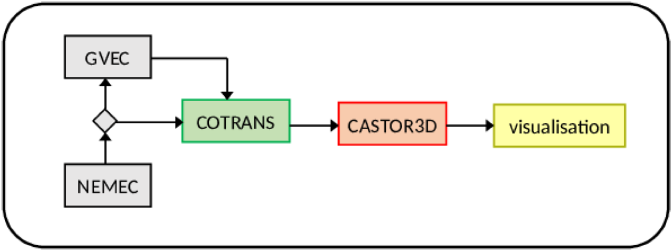

 R,φ,Z
 s,v,u
 u
 v
 s=1
 v
 Φ0/Φ0tot
 Φ0
 Φ0tot


 𝘼ext
 𝘽ext
 𝘼ext
 𝘽ext
 f,f~=ρ^,v^s,v^u,v^v,T^,A^s,A^u,A^v
 Nmn×Nmn
 q,q~=1,2

 n=40
 n=20
 s

 n∗=1
 fRe
 f~Re
 μ‖

 γ
 |ω|
 αs
 γideal
 |ωi∗|/2

 n∗=6
 e
 m/n
 R
 Z
 φ=0o
 t=0

 β
 η=10−7
 η=10−6
 η=10−7
 η=10−6

 αT
 αT
 ωi∗

 n∗=1,2,…,8
 Δs
 n∗=1
 ι
 W7-X

 n∗=1
 ηa
 n∗=1
 ηa=6×10⁻⁶
 ηa=6×10⁻⁵

 n∗=1
 n∗

 n∗=1
 ω<0

 Nper=2

 n∗=1
 σ3D,N
 Re(B1,⊥2)
 n∗=1
 Re(B1,⊥2)

 Re(B1,⊥eiφ)2
 n∗=15
 φ=0
 E=maxφ{Re(B1,⊥eiφ)2}
 σ3D,N
 E
 n∗=15
 n∗
 ωt∈[0,2πn∗]
 n∗

 #
 #
 #
 #
 n∗

 n∗
 n∗

 n∗=2
 n∗=22
 Ω0ext
 μ||=4 kg ms−1
 n∗=2

 η=6×10⁻⁷

 n∗=1↔n∗=9
 μ||=1.1 kg ms−1

 rc

 n∗=2
 dw
 Ω0=200000 rad s−1
 Ω0=50000 rad s−1

 #

 sj⩽s⩽sj+1

 Open access

