2 The setting

We will start by recalling some needed notions. In a more general situation such an exposition has already been given in [Reference Schmidt and Summerer5]. We will thus content ourselves to present it here for the two-dimensional approximation problem. Let $\unicode[STIX]{x1D6E5}\subseteq \mathbb{R}^{3}$ consist of the points $(\unicode[STIX]{x1D6FC}_{1},\unicode[STIX]{x1D6FC}_{2},\unicode[STIX]{x1D6FC}_{3})$ with $\unicode[STIX]{x1D6FC}_{1}\leqslant \unicode[STIX]{x1D6FC}_{2}\leqslant \unicode[STIX]{x1D6FC}_{3}$ . Observe that ${\mathcal{L}}_{\unicode[STIX]{x1D709}}:=(L_{1},L_{2},L_{3})$ with $L_{1},L_{2},L_{3}$ as in §1 is a map $(0,\infty )\rightarrow \unicode[STIX]{x1D6E5}$ .

A 3-system will be a map ${\mathcal{P}}:(0,\infty )\rightarrow \unicode[STIX]{x1D6E5}$ , where ${\mathcal{P}}=(P_{1},P_{2},P_{3})$ with each $P_{i}$ continuous and piecewise linear with slopes among $1,-2$ with $P_{1}(q)+P_{2}(q)+P_{3}(q)=0$ , and with a further condition formulated below.

The combined graph of ${\mathcal{P}}$ is the union of the graphs of $P_{1},P_{2},P_{3}$ . When for some point $(q,y)$ in the combined graph of ${\mathcal{P}}$ the set of slopes of the graph emanating to the left of $(q,y)$ is not the same as the set of slopes to the right, then $q$ is called a switch number. There will be some $P_{u}$ which changes slope at $q$ , and since $P_{1}+P_{2}+P_{3}=0$ there will be some $P_{v}$ , $v\neq u$ , which changes slope the “other way”. Say $P_{u}$ changes from rising to falling, $P_{v}$ from falling to rising. For a $3$ -system the extra condition alluded to above is in this case always $u>v$ . For given $u>v$ , the number $q$ is named a switch number of type $\binom{u}{v}$ . As a consequence, when $P_{1}$ has a local maximum at $q$ , then also the graph of $P_{2}$ passes through $(q,P_{1}(q))$ and $P_{1}(q)=P_{2}(q)$ ; when $P_{3}$ has a local minimum at $q$ , then $P_{2}(q)=P_{3}(q)$ .

Call ${\mathcal{P}}$ proper if $q-P_{3}(q)$ tends to infinity with $q$ . Call ${\mathcal{P}}$ agreeable if there is no $q$ with $P_{1}(q)=P_{2}(q)=P_{3}(q)$ (hence $=0$ ), and there is no interval of positive length where $P_{1}(q)=P_{2}(q)$ or $P_{2}(q)=P_{3}(q)$ .

The argument in the above proof shows that if $P_{2}(r)=P_{3}(r)$ and $P_{1}(r^{\ast })=P_{2}(r^{\ast })$ for certain arbitrarily large $r,r^{\ast }$ , then a $3$ -system ${\mathcal{P}}$ is proper. Conversely, when ${\mathcal{P}}$ is proper, then there are intervals $[s,r]$ with large $s$ where $P_{3}$ declines, and has a local minimum at $r$ , so that $P_{2}(r)=P_{3}(r)$ . Now $P_{1}(r)=P_{2}(r)=P_{3}(r)$ , or $P_{2}$ declines to the right of $r$ , hence $P_{1}$ inclines, and reaches a local maximum at some $r^{\ast }$ , so that $P_{1}(r^{\ast })=P_{2}(r^{\ast })$ .

We set $\unicode[STIX]{x1D711}_{i}(q):=P_{i}(q)/q$ for $i=1,2,3$ and note that the quantities $\text{}\underline{\unicode[STIX]{x1D711}}_{i}$ and $\overline{\unicode[STIX]{x1D711}}_{i}$ defined by (1.4) in terms of ${\mathcal{P}}$ are the same as the quantities defined in terms of ${\mathcal{L}}_{\unicode[STIX]{x1D709}}$ when ${\mathcal{P}}-{\mathcal{L}}_{\boldsymbol{\unicode[STIX]{x1D709}}}$ is bounded. By Theorem 2.1, to prove Theorem 1.1 up to the best possible assertion, we may deal with an agreeable, proper $3$ -system ${\mathcal{P}}$ . For such a system, the numbers $r$ with $P_{2}(r)=P_{3}(r)$ form a sequence tending to infinity, and so do the numbers $r^{\ast }$ with $P_{1}(r^{\ast })=P_{2}(r^{\ast })$ , and these sequences have no common element. In the mixed combined sequence of these $r^{\ast }$ and $r$ arranged in increasing order, blocks of $r^{\ast }$ will alternate with blocks of $r$ (possibly reduced to one single $r^{\ast }$ respectively  $r$ ). Starting with a block of $r^{\ast }$ , in the $j$ th block of $r^{\ast }$ denote the first and last element by $b_{j}^{\ast }$ and $a_{j}^{\ast }$ . In the directly following block of $r$ denote the first and last element by $a_{j}$ and $b_{j}$ . Note that if $b_{j}^{\ast }=a_{j}^{\ast }$ or $a_{j}=b_{j}$ , then the corresponding block consists of only one element. Set ${\mathcal{I}}_{j}:=[b_{j-1},b_{j+1}^{\ast }]$ , and note that ${\mathcal{I}}_{j},{\mathcal{I}}_{j+1}$ overlap on $[b_{j},b_{j+1}^{\ast }]$ .

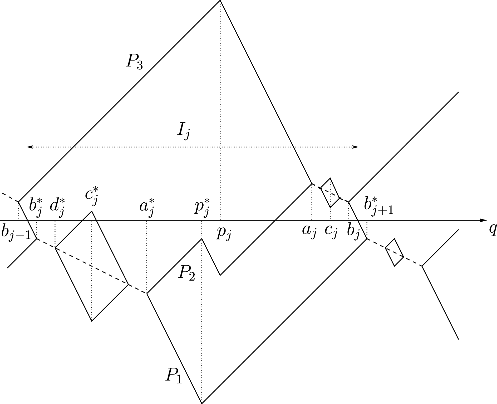
In $(a_{j}^{\ast },b_{j+1}^{\ast })$ we have $P_{1}(q)\neq P_{2}(q)$ , so that $P_{1}$ has no local maximum. $P_{1}$ decreases up to some $p_{j}^{\ast }$ , then increases. Similarly, $P_{3}$ increases up to some $p_{j}$ , then decreases up to $a_{j}$ . In the case when $P_{2}$ increases throughout $[a_{j}^{\ast },a_{j}]$ , then $p_{j}=p_{j}^{\ast }$ and this number is a switch number of type $\binom{3}{1}$ . Otherwise, $P_{2}$ increases in $[a_{j}^{\ast },p_{j}^{\ast }]$ , decreases in $[p_{j}^{\ast },p_{j}]$ where $p_{j}^{\ast }<p_{j}$ , and increases in $[p_{j},a_{j}]$ . In this case $p_{j}^{\ast },p_{j}$ are respectively switch numbers of type $\binom{2}{1}$ and $\binom{3}{2}$ .

When $b_{j}^{\ast }<a_{j}^{\ast }$ , then ${\textstyle \frac{1}{2}}(P_{1}+P_{2})$ will decrease in $(b_{j}^{\ast },a_{j}^{\ast })$ with slope $-1/2$ , and $P_{1},P_{2}$ will zigzag around the dotted line of Figure 1. Any local minimum of $P_{1}$ in the interval will be assumed at a switch number of type $\binom{2}{1}$ . Similarly, when $a_{j}<b_{j}$ , then $P_{2},P_{3}$ will zigzag around a line of slope $-1/2$ and a local maximum of $P_{3}$ in $[a_{j},b_{j}]$ will be asumed at a switch number of type $\binom{3}{2}$ .

For the convenience of the reader we illustrate the described situation within some interval ${\mathcal{I}}_{j}$ in Figure 1.

Figure 1

Now let $c_{j}^{\ast }\in {\mathcal{I}}_{j}$ be a number where $P_{1}$ assumes a local minimum. Then $b_{j}^{\ast }<c_{j}^{\ast }\leqslant p_{j}^{\ast }$ . We will always have such a local minimum within $[a_{j}^{\ast },a_{j}]$ , namely at $c_{j}^{\ast }=p_{j}^{\ast }$ and when $b_{j}^{\ast }<a_{j}^{\ast }$ there will be at least one more such $c_{j}^{\ast }$ within $(b_{j}^{\ast },a_{j}^{\ast })$ . For any $c_{j}^{\ast }\in (b_{j}^{\ast },a_{j}^{\ast })$ let $d_{j}^{\ast }<c_{j}^{\ast }$ be the largest number where $P_{1}(d_{j}^{\ast })=P_{2}(d_{j}^{\ast })$ . For $c_{j}^{\ast }=p_{j}^{\ast }$ let $d_{j}^{\ast }=a_{j}^{\ast }$ .

Let $c_{j}\in {\mathcal{I}}_{j}$ be a number where $P_{3}$ assumes a local maximum. Then $p_{j}\leqslant c_{j}<b_{j}$ . Thus $c_{j}$ may be $p_{j}$ , and when $a_{j}<b_{j}$ there will be at least one such $c_{j}$ within $(a_{j},b_{j})$ . For any $c_{j}\in (a_{j},b_{j})$ let $d_{j}>c_{j}$ be the least number where $P_{3}(d_{j})=P_{2}(d_{j})$ . For $c_{j}=p_{j}$ let $d_{j}=a_{j}$ .

Let $\overline{\unicode[STIX]{x1D711}}_{ij}$ be the maximum of $\unicode[STIX]{x1D711}_{i}$ in ${\mathcal{I}}_{j}$ respectively $\text{}\underline{\unicode[STIX]{x1D711}}_{ij}$ the minimum. Note that when $\overline{\unicode[STIX]{x1D719}}_{i}>\overline{\unicode[STIX]{x1D711}}_{i}$ , $\text{}\underline{\unicode[STIX]{x1D719}}_{i}<\text{}\underline{\unicode[STIX]{x1D711}}_{i}$ , then $\overline{\unicode[STIX]{x1D711}}_{ij}<\overline{\unicode[STIX]{x1D719}}_{i}$ , $\text{}\underline{\unicode[STIX]{x1D711}}_{ij}>\text{}\underline{\unicode[STIX]{x1D719}}_{i}$ when $j$ is large.

In what follows, we will assume

3 Basic inequalities

In this section we derive a few relations that result from the basic properties of proper 3-systems, in particular from $P_{1}+P_{2}+P_{3}=0$ and the knowledge of the possible slopes for these functions.

For any $c_{j}^{\ast }$ as defined in Section 2 we have

and therefore

hence upon division by $c_{j}^{\ast }$

Also

and division by $c_{j}^{\ast }$ yields

Combining (3.1) and (3.2) we obtain

since $\unicode[STIX]{x1D711}_{1}(b_{j}^{\ast })\geqslant -1/2$ . Here

in view of $\unicode[STIX]{x1D711}_{1}(c_{j}^{\ast })\geqslant -2$ and $\unicode[STIX]{x1D711}_{2}(c_{j}^{\ast })\leqslant 1$ . Moreover $\unicode[STIX]{x1D711}_{1}(b_{j}^{\ast })\leqslant \overline{\unicode[STIX]{x1D719}}_{1}$ , so that

which may also be written as

Thus $(\unicode[STIX]{x1D711}_{1}(c_{j}^{\ast }),\unicode[STIX]{x1D711}_{3}(c_{j}^{\ast }))$ lies on or above the line $L^{\ast }$ with equation

Dually to (3.4),

so that $(\unicode[STIX]{x1D711}_{1}(c_{j}),\unicode[STIX]{x1D711}_{3}(c_{j}))$ lies on or below the line $L$ with equation

Now choose $c_{j}^{\ast }$ to be a number where $\unicode[STIX]{x1D711}_{1}$ assumes its minimum in ${\mathcal{I}}_{j}$ . Then $\unicode[STIX]{x1D711}_{1}(c_{j}^{\ast })=\text{}\underline{\unicode[STIX]{x1D711}}_{1j}$ and $\unicode[STIX]{x1D711}_{3}(c_{j}^{\ast })<\overline{\unicode[STIX]{x1D719}}_{3}$ , so that (3.4) yields

Since $\text{}\underline{\unicode[STIX]{x1D711}}_{1}=\liminf _{j}\text{}\underline{\unicode[STIX]{x1D711}}_{1j}$ , we obtain

or, since $\overline{\unicode[STIX]{x1D719}}_{i}$ may be chosen arbitrarily close to $\overline{\unicode[STIX]{x1D711}}_{i}$ for $i=1,3$ ,

DuallyFootnote ¹ to (3.6),

4 Bounds for $\overline{\unicode[STIX]{x1D711}}_{2j}$ and $\text{}\underline{\unicode[STIX]{x1D711}}_{2j}$

$\unicode[STIX]{x1D711}_{2}$ does have local maxima where $P_{2}$ does. In ${\mathcal{I}}_{j}$ these local maxima are at $a_{j}$ , at $p_{j}^{\ast }$ if $p_{j}^{\ast }<p_{j}$ and at numbers $c_{j}^{\ast }$ in $(b_{j}^{\ast },a_{j}^{\ast })$ .

The point $(a_{j},P_{2}(a_{j}))$ is the intersection of the line of slope $1$ through $(p_{j},P_{2}(p_{j}))$ and the line of slope $-2$ through $(p_{j},P_{3}(p_{j}))$ . Therefore

and also

Twice the first of these equations added to the second gives

Moreover

by Figure 1, so that

so that in combination with (4.1)

with

Since $f(x,y)$ is decreasing in $x$ as well as in $y$ when $3+x+2y>0$ , and since $\unicode[STIX]{x1D711}_{1}(p_{j})\geqslant \unicode[STIX]{x1D711}_{1}(p_{j}^{\ast })$ , $\unicode[STIX]{x1D711}_{3}(p_{j})\geqslant \unicode[STIX]{x1D711}_{3}(p_{j}^{\ast })$ , we obtain

Given $c_{j}^{\ast }\in (b_{j}^{\ast },a_{j}^{\ast })$ , let $(\tilde{a}_{j},\tilde{P}_{j})$ be the point of intersection of the line of slope $1$ through $(c_{j}^{\ast },P_{2}(c_{j}^{\ast }))$ and the line of slope $-2$ through $(c_{j}^{\ast },P_{3}(c_{j}^{\ast }))$ . By the argument above, with $c_{j}^{\ast }$ in place of $p_{j}$ we obtain, in analogy to (4.3)

where $\tilde{\unicode[STIX]{x1D711}}_{2}(\tilde{a}_{j})=\tilde{P}_{j}/\tilde{a}_{j}$ . Since clearly $\unicode[STIX]{x1D711}_{2}(c_{j}^{\ast })\leqslant \tilde{\unicode[STIX]{x1D711}}_{2}(\tilde{a}_{j})$ , we may conclude that $\unicode[STIX]{x1D711}_{2}(c_{j}^{\ast })\leqslant f(\unicode[STIX]{x1D711}_{1}(c_{j}^{\ast }),\unicode[STIX]{x1D711}_{3}(c_{j}^{\ast }))$ , hence (as $p_{j}^{\ast }$ is also some $c_{j}^{\ast }$ )

and therefore

with the maximum ranging over points $(x,y)$ on or above $L^{\ast }$ and with $x\geqslant \text{}\underline{\unicode[STIX]{x1D719}}_{1}$ .

Dually to (4.3), (4.6)

with $f^{\ast }(x,y)=f(y,x)=-(2y+x)/(3+y+2x)$ , and

with the minimum ranging over points on or below $L$ , and with $y\leqslant \overline{\unicode[STIX]{x1D719}}_{3}$ .

5 Proof of (1.8) and (1.9)

Since $f(x,y)$ increases as $y$ decreases, $f(x,y)$ with $(x,y)$ as in (4.6) is ${\leqslant}f(x,y(x))$ with $x\geqslant \text{}\underline{\unicode[STIX]{x1D719}}_{1}$ , where $L^{\ast }$ is given by

Hence we obtain

and simplification leads to

Since $x\geqslant \text{}\underline{\unicode[STIX]{x1D719}}_{1}$ , this is at most $(-\text{}\underline{\unicode[STIX]{x1D719}}_{1}+\overline{\unicode[STIX]{x1D719}}_{1})/(2-\overline{\unicode[STIX]{x1D719}}_{1}-\overline{\unicode[STIX]{x1D719}}_{1}\text{}\underline{\unicode[STIX]{x1D719}}_{1})$ , which is therefore an upper bound for $\unicode[STIX]{x1D711}_{2j}$ . This is also an upper bound for $\text{}\underline{\unicode[STIX]{x1D711}}_{2}$ , and since $\overline{\unicode[STIX]{x1D719}}_{1},\text{}\underline{\unicode[STIX]{x1D719}}_{1}$ can be chosen arbitrarily close to $\overline{\unicode[STIX]{x1D711}}_{1},\text{}\underline{\unicode[STIX]{x1D711}}_{1}$ , inequality (1.8) follows.

Here $f^{\ast }(x,y)$ decreases as $x$ increases, so that $f^{\ast }(x,y)$ with $(x,y)$ as in (4.6*) is ${\geqslant}f^{\ast }(x(y),y)$ where $L$ consists of points $(x(y),y)$ . Dually to (5.1)

Taking into account $y\leqslant \overline{\unicode[STIX]{x1D719}}_{3}$ , inequality (1.9) easily follows.

6 Standard pieces

Before turning to the “best possible” assertion of Theorem 1.1 we need to define standard functions on some intervals.

Suppose $\text{}\underline{\unicode[STIX]{x1D711}}_{1}\overline{\unicode[STIX]{x1D711}}_{1},\text{}\underline{\unicode[STIX]{x1D711}}_{2},\overline{\unicode[STIX]{x1D711}}_{2},\text{}\underline{\unicode[STIX]{x1D711}}_{3},\overline{\unicode[STIX]{x1D711}}_{3}$ are numbers with (1.5), $\ldots$  , (1.9) and with $\text{}\underline{\unicode[STIX]{x1D711}}_{3}<1$ (hence $\overline{\unicode[STIX]{x1D711}}_{1}>-1/2$ ) and $\text{}\underline{\unicode[STIX]{x1D711}}_{1}<0<\overline{\unicode[STIX]{x1D711}}_{3}$ . Further let $\text{}\underline{t},\overline{t}$ be numbers, not both zero, with $\overline{t}<1$ ,

so that (1.7) holds with $\text{}\underline{t},\overline{t}$ in place of $\text{}\underline{\unicode[STIX]{x1D711}}_{1},\overline{\unicode[STIX]{x1D711}}_{3}$ . Thus $(\text{}\underline{t},\overline{t})$ is on or below the line $L$ given by $(2+\text{}\underline{\unicode[STIX]{x1D711}}_{3})x+(1+2\text{}\underline{\unicode[STIX]{x1D711}}_{3})y=-3\text{}\underline{\unicode[STIX]{x1D711}}_{3}$ , and on or above the line $L^{\ast }$ with equation $(1+2\overline{\unicode[STIX]{x1D711}}_{1})x+(2+\overline{\unicode[STIX]{x1D711}}_{1})y=-3\overline{\unicode[STIX]{x1D711}}_{1}$ . (Note that $L,L^{\ast }$ are analogues to the lines of §3.) So $(\text{}\underline{t},\overline{t})$ is also on or below the line $y=1$ , hence is in the triangle $T$ bounded by these three lines. A short computation shows that the vertices of $T$ are $(-2,1)$ , $(\unicode[STIX]{x1D6FC},1)$ with $\unicode[STIX]{x1D6FC}:=-(1+5\text{}\underline{\unicode[STIX]{x1D711}}_{3})/(2+\text{}\underline{\unicode[STIX]{x1D711}}_{3})>-2$ and $(\text{}\underline{\unicode[STIX]{x1D6FD}},\bar{\unicode[STIX]{x1D6FD}})$ with $\text{}\underline{\unicode[STIX]{x1D6FD}}:=-3\text{}\underline{\unicode[STIX]{x1D711}}_{3}/(1-\overline{\unicode[STIX]{x1D711}}_{1}\text{}\underline{\unicode[STIX]{x1D711}}_{3})$ , $\bar{\unicode[STIX]{x1D6FD}}:=-3\overline{\unicode[STIX]{x1D711}}_{1}/(1-\overline{\unicode[STIX]{x1D711}}_{1}\text{}\underline{\unicode[STIX]{x1D711}}_{3})$ , so that $\text{}\underline{\unicode[STIX]{x1D6FD}}\leqslant 0,\bar{\unicode[STIX]{x1D6FD}}\geqslant 0$ and

By (6.1),

hence $2\overline{t}+\text{}\underline{t}\geqslant 0$ . Dually, $2\text{}\underline{t}+\overline{t}\leqslant 0$ , so that

Not both relations can hold with equality, for then $\text{}\underline{t}=\overline{t}=0$ , which was ruled out. We may infer that $\text{}\underline{t}<0<\overline{t}$ . The case where both relations in (6.3) are strict inequalities will be called the generic case, the other case is the special case. This case can only occur when $\overline{\unicode[STIX]{x1D711}}_{1}=0=\text{}\underline{\unicode[STIX]{x1D711}}_{3}$ .

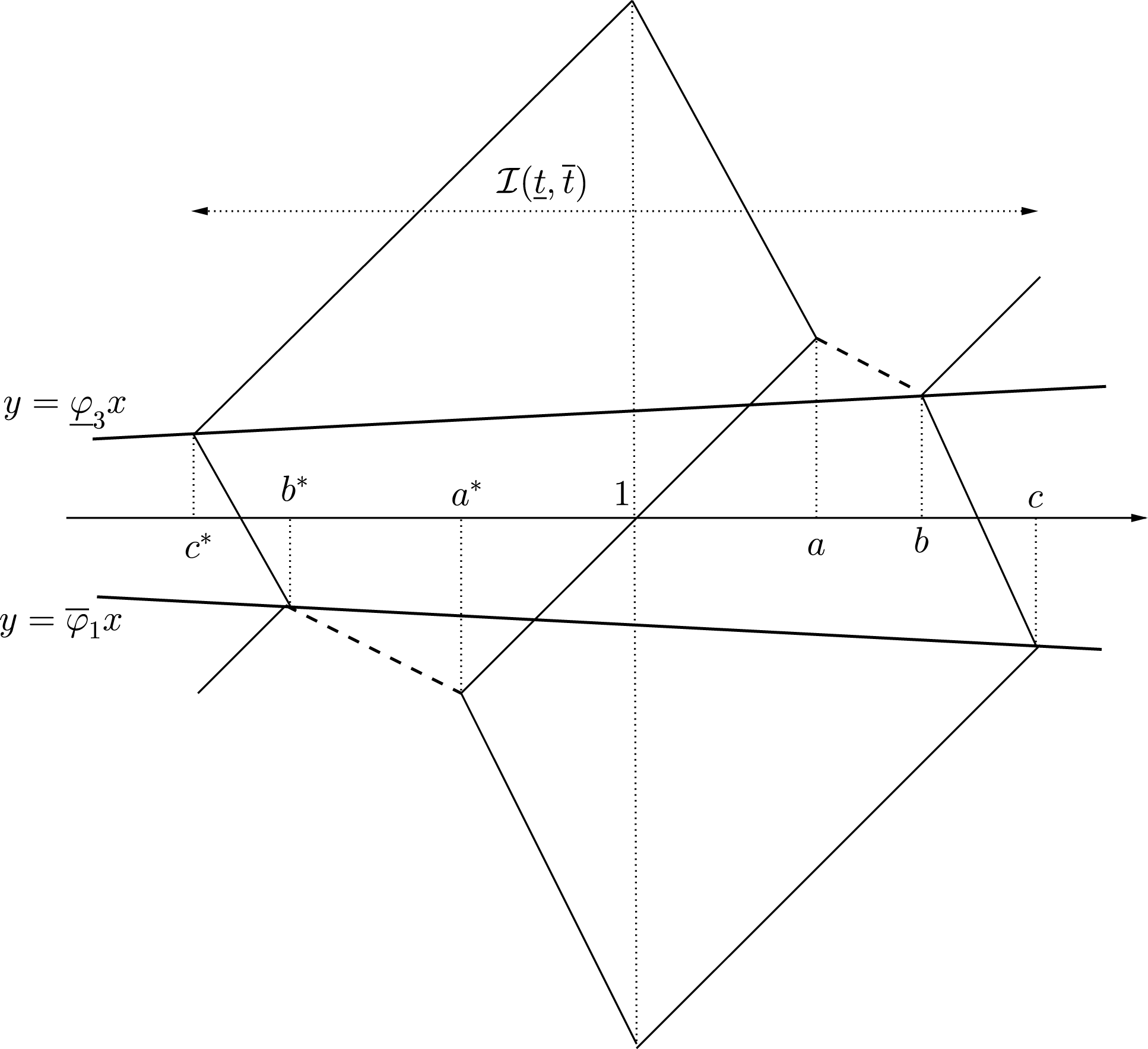
After this tedious beginning we now come to the core of this section. For suitable numbers

with $c^{\ast }<c$ (which have no relation with the numbers $c_{j}^{\ast },c_{j}$ of §3) we will construct functions $P_{1},P_{2},P_{3}$ on ${\mathcal{I}}(\text{}\underline{t},\overline{t}):=[c^{\ast },c]$ with $P_{1}+P_{2}+P_{3}=0$ , where each $P_{i}$ is continuous and piecewise linear with slopes among $1,-2$ . We will have

$P_{1}$ will rise (with slope $1$ ) in $[1,c]$ . $P_{2}$ will rise, $P_{3}$ will fall (with slope $-2$ ) to the right of $q=1$ , and they will meet at $q=a$ , so that $P_{2}(a)=P_{3}(a)$ . Since

and also

we obtain

in fact ${>}1$ when $2\overline{t}+\text{}\underline{t}>0$ . It follows that

Moreover $P_{2}(b)=P_{3}(b)=\text{}\underline{\unicode[STIX]{x1D711}}_{3}b$ , and when $a<b$ , then $P_{2},P_{3}$ will zigzag with alternating slopes $1,-2$ around a line of slope $-1/2$ (indicated by a dotted line segment in Figure 2), so that

hence

so that

Finally $P_{1}(c)=P_{2}(c)$ , and when $b<c$ , then $P_{1},P_{3}$ will rise, $P_{2}$ will fall in $[b,c]$ . Since $P_{1}(b)=-2P_{2}(b)=-2\text{}\underline{\unicode[STIX]{x1D711}}_{3}b$ , we have $3(c-b)=P_{3}(b)-P_{1}(b)=-3\text{}\underline{\unicode[STIX]{x1D711}}_{3}b$ , hence $c=(1+\text{}\underline{\unicode[STIX]{x1D711}}_{3})b$ , $c>b$ if $\text{}\underline{\unicode[STIX]{x1D711}}_{3}>0$ . Moreover by (6.8), (1.6)

Also $P_{2}(c)=P_{3}(b)-2(c-b)=\text{}\underline{\unicode[STIX]{x1D711}}_{3}b-2\text{}\underline{\unicode[STIX]{x1D711}}_{3}b=-\text{}\underline{\unicode[STIX]{x1D711}}_{3}b$ . So

But $P_{1}(c)=\text{}\underline{t}+c-1$ since $P_{1}$ rises in $[1,c]$ , and we obtain again (6.9). By (6.7), (6.8), (6.1),

Figure 2

We give a dual construction on the left of $q=1$ . In our duality, we have $c^{\ast },b^{\ast },a^{\ast }$ in place of $c,b,a$ , and $\overline{\unicode[STIX]{x1D711}}_{1},\text{}\underline{\unicode[STIX]{x1D711}}_{3},\overline{t},\text{}\underline{t},P_{1},P_{2},P_{3}$ are replaced by $\text{}\underline{\unicode[STIX]{x1D711}}_{3},\overline{\unicode[STIX]{x1D711}}_{1},\text{}\underline{t},\overline{t},P_{3},P_{2},P_{1}$ . Now $P_{3}$ rises in $[c^{\ast },1]$ , $P_{1}(a^{\ast })=P_{2}(a^{\ast })$ and $P_{2}$ rises, $P_{1}$ falls in $[a^{\ast },1]$ . Hence

Also

and

By (6.6), (6.8), (6.9), (6.6*), (6.8*), (6.9*) (and using (6.3)) we have in fact (6.4). Not both relations $a=1$ and $a^{\ast }=1$ can hold, so that $a^{\ast }<a$ , hence $c^{\ast }<c$ .

The triple of functions on the interval ${\mathcal{I}}(\text{}\underline{t},\overline{t})$ will be called a standard piece and denoted ${\mathcal{P}}(\text{}\underline{t},\overline{t})$ . When $\overline{\unicode[STIX]{x1D711}}_{1}=0=\text{}\underline{\unicode[STIX]{x1D711}}_{3}$ , then $c^{\ast }=b^{\ast }$ , $b=c$ , and $P_{1}(q)=P_{2}(q)=P_{3}(q)=0$ for $q=c^{\ast }$ and $q=c$ . Moreover there will be an interval $[c^{\ast },g^{\ast }]$ with $c^{\ast }<g^{\ast }$ where $P_{1}(q)=P_{2}(q)$ , and an interval $[g,c]$ with $g<c$ where $P_{2}(q)=P_{3}(q)$ . A degenerate version of Figure 2 will ensue.

Define $\unicode[STIX]{x1D711}_{i}(q)=P_{i}(q)/q$ for $i=1,2,3$ on ${\mathcal{I}}(\text{}\underline{t},\overline{t})$ , and let $\overline{\unicode[STIX]{x1D711}}_{i}({\mathcal{P}}(\text{}\underline{t},\overline{t}))$ (respectively $\text{}\underline{\unicode[STIX]{x1D711}}_{i}({\mathcal{P}}(\text{}\underline{t},\overline{t}))$ ) be the maximum (respectively minimum) of $\unicode[STIX]{x1D711}_{i}(q)$ in ${\mathcal{I}}(\text{}\underline{t},\overline{t})$ . Clearly $\text{}\underline{\unicode[STIX]{x1D711}}_{3}({\mathcal{P}}(\text{}\underline{t},\overline{t}))=\text{}\underline{\unicode[STIX]{x1D711}}_{3}$ and $\overline{\unicode[STIX]{x1D711}}_{1}({\mathcal{P}}(\text{}\underline{t},\overline{t}))=\overline{\unicode[STIX]{x1D711}}_{1}$ . But caution: ${\mathcal{P}}(\text{}\underline{t},\overline{t})$ is not completely determined if $b^{\ast }<a^{\ast }$ or $a<b$ . In the generic case, $a^{\ast }<1<a$ , $P_{1}(a^{\ast })>\text{}\underline{t}$ , $P_{3}(a)<\overline{t}$ , and we can pick alternating functions in $[b^{\ast },a^{\ast }]$ and $[a,b]$ such that $\text{}\underline{\unicode[STIX]{x1D711}}_{1}({\mathcal{P}}(\text{}\underline{t},\overline{t}))=\text{}\underline{t}$ , $\overline{\unicode[STIX]{x1D711}}_{3}({\mathcal{P}}(\text{}\underline{t},\overline{t}))=\overline{t}$ . In the special case we can for each $\unicode[STIX]{x1D716}>0$ pick a standard piece ${\mathcal{P}}_{\unicode[STIX]{x1D716}}(\text{}\underline{t},\overline{t})\!)$ with

We will now suppose $\overline{\unicode[STIX]{x1D711}}_{3}<1$ , hence $\text{}\underline{\unicode[STIX]{x1D711}}_{1}<0<\overline{\unicode[STIX]{x1D711}}_{3}<1$ . Three choices for $(\text{}\underline{t},\overline{t})$ will be needed, denoted by $(\text{}\underline{s}_{j},\overline{s}_{j})$ for $j=0,1,2$ . First

which is allowed by (1.7). Here

in the generic case,

in the special case.

Next,

where $y=y(x)$ is the equation of the line $L^{\ast }$ . Thus $(\text{}\underline{s}_{1},\overline{s}_{1})$ is the downward projection of $(\text{}\underline{\unicode[STIX]{x1D711}}_{1},\overline{\unicode[STIX]{x1D711}}_{3})$ on $L^{\ast }$ , hence is in $T$ , hence satisfies the condition on pairs $(\text{}\underline{t},\overline{t})$ . Moreover $y(\text{}\underline{\unicode[STIX]{x1D711}}_{1})\leqslant \overline{\unicode[STIX]{x1D711}}_{3}$ , so that

respectively

in the generic respectively in the special case for sufficiently small $\unicode[STIX]{x1D716}$ .

Moreover by (4.3) with $p_{j}=1$ , and by (6.5),

hence by (5.1)

with $\bar{\unicode[STIX]{x1D6FA}}$ as in (1.8).

Finally,

where $x=x(y)$ is the equation of $L$ . By an argument dual to the one for $(\text{}\underline{s}_{1},\overline{s}_{1})$ ,

in the general and the special case. By (4.3*) with $p_{j}^{\ast }=1$ ,

so that by (5.1*)

${\mathcal{P}}(\text{}\underline{s}_{0},\overline{s}_{0})$ is agreeable in an obvious sense unless $\text{}\underline{\unicode[STIX]{x1D711}}_{1}+2\overline{\unicode[STIX]{x1D711}}_{3}=0$ or $2\text{}\underline{\unicode[STIX]{x1D711}}_{1}+\overline{\unicode[STIX]{x1D711}}_{3}=0$ , and ${\mathcal{P}}(\text{}\underline{s}_{1},\overline{s}_{1})$ , ${\mathcal{P}}(\text{}\underline{s}_{2},\overline{s}_{2})$ are agreeable when $\overline{\unicode[STIX]{x1D711}}_{1}<0<\text{}\underline{\unicode[STIX]{x1D711}}_{3}$ but not otherwise, since $\overline{\unicode[STIX]{x1D711}}_{1}=0=\text{}\underline{\unicode[STIX]{x1D711}}_{3}$ implies $y(\overline{\unicode[STIX]{x1D711}}_{1})=-{\textstyle \frac{1}{2}}\overline{\unicode[STIX]{x1D711}}_{1}$ , $x(\overline{\unicode[STIX]{x1D711}}_{3})=-12\overline{\unicode[STIX]{x1D711}}_{3}$ .

7 Best possible

Given a $3$ -system ${\mathcal{P}}$ we had in §2 defined quantities $\text{}\underline{\unicode[STIX]{x1D711}}_{i},\overline{\unicode[STIX]{x1D711}}_{i}$ , $i=1,2,3$ , which will now be denoted $\text{}\underline{\unicode[STIX]{x1D711}}_{i}({\mathcal{P}}),\overline{\unicode[STIX]{x1D711}}_{i}({\mathcal{P}})$ . To prove that the conditions (1.5), $\ldots$  , (1.9) are best possible, we will for given numbers $\text{}\underline{\unicode[STIX]{x1D711}}_{i},\overline{\unicode[STIX]{x1D711}}_{i}$ satisfying these five conditions, as well as $\text{}\underline{\unicode[STIX]{x1D711}}_{3}<1$ , construct a proper $3$ -system ${\mathcal{P}}$ with

and

with $\text{}\underline{\unicode[STIX]{x1D6FA}},\overline{\unicode[STIX]{x1D6FA}}$ as in (1.8), (1.9). In the generic case, when (6.3) holds with strict inequalities, ${\mathcal{P}}$ will be self-similar, i.e. will be invariant under dilation by a factor $\unicode[STIX]{x1D70C}>1$ .

When ${\mathcal{P}}(\text{}\underline{t},\overline{t})$ is as in the preceding section, let ${\mathcal{P}}^{-}(\text{}\underline{t},\overline{t})$ (respectively ${\mathcal{P}}^{+}(\text{}\underline{t},\overline{t})$ ) be its part with $q\in [c^{\ast },b^{\ast }]$ (respectively $q\in [b,c]$ ). For any $(\text{}\underline{t},\overline{t}),(\text{}\underline{t}^{\prime },\overline{t}^{\prime })$ , the parts ${\mathcal{P}}^{-}(\text{}\underline{t},\overline{t}),{\mathcal{P}}^{+}(\text{}\underline{t},\overline{t}),{\mathcal{P}}^{-}(\text{}\underline{t}^{\prime },\overline{t}^{\prime }),{\mathcal{P}}^{+}(\text{}\underline{t}^{\prime },\overline{t}^{\prime })$ will all be similar, i.e. obtained from each other by multiplication by factors $\unicode[STIX]{x1D70C}>0$ . In particular, ${\mathcal{P}}^{+}(\text{}\underline{t},\overline{t})$ is obtained from ${\mathcal{P}}^{-}(\text{}\underline{t},\overline{t})$ by a factor $\unicode[STIX]{x1D70C}(\text{}\underline{t},\overline{t})>1$ . In fact, $\unicode[STIX]{x1D70C}(\text{}\underline{t},\overline{t})=b/c^{\ast }=c/b^{\ast }$ .

Let $(\text{}\underline{t}_{j},\overline{t}_{j})$ , $j\in \mathbb{Z}$ , again be pairs with $\overline{t}_{j}\leqslant 1$ and with (6.1). Then

so that

defines functions on ${\mathcal{I}}(\text{}\underline{t}_{j},\overline{t}_{j})\cup \unicode[STIX]{x1D70C}(\text{}\underline{t}_{j},\overline{t}_{j}){\mathcal{I}}(\text{}\underline{t}_{j+1},\overline{t}_{j+1})$ : we could say that the standard pieces ${\mathcal{P}}(\text{}\underline{t}_{j},\overline{t}_{j})$ , ${\mathcal{P}}(\text{}\underline{t}_{j+1},\overline{t}_{j+1})$ are patched together. Define $\unicode[STIX]{x1D714}_{j}$ ( $j\in \mathbb{Z}$ ) by $\unicode[STIX]{x1D714}_{0}=1$ and $\unicode[STIX]{x1D714}_{j+1}/\unicode[STIX]{x1D714}_{j}=\unicode[STIX]{x1D70C}(\text{}\underline{t}_{j},\overline{t}_{j})$ . If $\unicode[STIX]{x1D714}_{j}\rightarrow 0$ (respectively $\unicode[STIX]{x1D714}_{j}\rightarrow \infty$ ) as $j\rightarrow -\infty$ (respectively $j\rightarrow \infty$ ), then

defines a proper 3-system on $(0,\infty )$ .

Again suppose $\text{}\underline{\unicode[STIX]{x1D711}}_{1}<0<\overline{\unicode[STIX]{x1D711}}_{3}<1$ . We now set $(\text{}\underline{t}_{j},\overline{t}_{j})=(\text{}\underline{s}_{i},\overline{s}_{i})$ for $i=0,1,2$ when $j\equiv i(\text{mod}\,3)$ . In the case when $\overline{\unicode[STIX]{x1D711}}_{1}<0<\text{}\underline{\unicode[STIX]{x1D711}}_{3}$ , it follows from (6.12), (6.15), (6.17), (6.15*), (6.17*) and the bounds (1.8), (1.9) that (7.1), (7.2) hold. Our ${\mathcal{P}}$ is agreeable and self similar with factor $\unicode[STIX]{x1D70C}:=\unicode[STIX]{x1D70C}(\text{}\underline{s}_{0},\overline{s}_{0})\unicode[STIX]{x1D70C}(\text{}\underline{s}_{1},\overline{s}_{1})\unicode[STIX]{x1D70C}(\text{}\underline{s}_{2},\overline{s}_{2})$ . In the case when $\overline{\unicode[STIX]{x1D711}}_{1}=0=\text{}\underline{\unicode[STIX]{x1D711}}_{3}$ we pick $\unicode[STIX]{x1D716}_{j}>0$ with $\unicode[STIX]{x1D716}_{j}\rightarrow 0$ as $j\rightarrow \infty$ , and in (7.3) replace ${\mathcal{P}}(\text{}\underline{t}_{j},\overline{t}_{j})$ by ${\mathcal{P}}_{\unicode[STIX]{x1D716}}(\text{}\underline{t}_{j},\overline{t}_{j})$ . Again (7.1), (7.2) will hold. Thus Theorem 1.1 is true when $\text{}\underline{\unicode[STIX]{x1D711}}_{1}<0<\overline{\unicode[STIX]{x1D711}}_{3}<1$ .

Next suppose $\text{}\underline{\unicode[STIX]{x1D711}}_{1}<0\leqslant \text{}\underline{\unicode[STIX]{x1D711}}_{3}<\overline{\unicode[STIX]{x1D711}}_{3}=1$ . Pick a sequence of points $(\text{}\underline{s}_{0j},\overline{s}_{0j})\in T$ tending to $(\text{}\underline{\unicode[STIX]{x1D711}}_{1},\overline{\unicode[STIX]{x1D711}}_{3})$ as $j\rightarrow \infty$ , with $\text{}\underline{s}_{0j}>\text{}\underline{\unicode[STIX]{x1D711}}_{1}$ , ${\textstyle \frac{1}{2}}(\text{}\underline{\unicode[STIX]{x1D711}}_{3}+\overline{\unicode[STIX]{x1D711}}_{3})<\overline{s}_{0j}<\overline{\unicode[STIX]{x1D711}}_{3}=1$ . Also set

so that for $i=0,1,2$ ,

where $(\text{}\underline{s}_{i},\overline{s}_{i})$ is given by (6.11), (6.14), (6.18). Set $(\text{}\underline{t}_{j},\overline{t}_{j})=(\text{}\underline{s}_{ij},\overline{s}_{ij})$ for $i=0,1,2$ when $j\equiv i(\text{mod}\,3)$ . When $j\equiv 0(\text{mod}\,3)$ , then (6.9*) with $\overline{t}_{j}$ in place of $\overline{t}$ yields

so that $\unicode[STIX]{x1D70C}(\text{}\underline{t}_{j},\overline{t}_{j})\geqslant 1-c_{j}^{\ast }>1-\unicode[STIX]{x1D713}>0$ . So if again ${\mathcal{P}}$ is defined by (7.3), with ${\mathcal{P}}(\text{}\underline{t}_{j},\overline{t}_{j})$ or ${\mathcal{P}}_{\unicode[STIX]{x1D716}}(\text{}\underline{t}_{j},\overline{t}_{j})$ , then again (7.1), (7.2) hold.

This takes care of the case when $\text{}\underline{\unicode[STIX]{x1D711}}_{1}<0<\overline{\unicode[STIX]{x1D711}}_{3}$ . Otherwise $\text{}\underline{\unicode[STIX]{x1D711}}_{1}=0=\overline{\unicode[STIX]{x1D711}}_{3}$ , and $\text{}\underline{\unicode[STIX]{x1D711}}_{i}=0=\overline{\unicode[STIX]{x1D711}}_{i}$ for $i=1,2,3$ . But as is well known, this is true for almost every $\boldsymbol{\unicode[STIX]{x1D709}}\in \mathbb{R}^{2}$ in the sense of Lebesgue measure. With a little effort one could construct a proper $3$ -system ${\mathcal{P}}$ with each $\text{}\underline{\unicode[STIX]{x1D711}}_{i}=\overline{\unicode[STIX]{x1D711}}_{i}=0$ . The proof of Theorem 1.1 is thus complete.

As for the remark below the Theorem, it is best possible since all the quantities $\text{}\underline{\unicode[STIX]{x1D711}}_{i},\overline{\unicode[STIX]{x1D711}}_{i}$ are completely described. But one really should prove that $\boldsymbol{\unicode[STIX]{x1D709}}=(\unicode[STIX]{x1D709}_{1},\unicode[STIX]{x1D709}_{2})$ with $1,\unicode[STIX]{x1D709}_{1},\unicode[STIX]{x1D709}_{2}$ linearly independent over $\mathbb{Q}$ with $\overline{\unicode[STIX]{x1D711}}_{3}=1$ exist. We invite the reader to construct a proper $3$ -system ${\mathcal{P}}$ with this property.