THE JOBS MODEL

The Jobs Model elaborates on the core Political Economy Model dominating the statistical forecasting literature (Lewis-Beck and Tien Reference Lewis-Beck, Tien, Clements and Hendry2011). It reads as follows: Vote = Presidential Popularity, Economic Growth × Incumbent Interaction, Jobs Creation, Incumbency Advantage. During recent US presidential elections, this model has been tested in numerous ways: first, in unconditional, ex ante trials, for each of these elections, and second subjected to multiple diagnostics. Of particular interest here is assessment of its step-ahead forecasting properties, compared to the baseline core Political Economy Model, vote = f (Presidential Popularity, Economic Growth). Seven elections (1984–2008) were forecast step-ahead, using this Core Model and our Jobs Model, that is, using 1952–1980 data, we forecasted 1984; then using 1952–1984 data, we forecasted 1988, and so on, through subsequent elections. The Jobs Model rendered a small step-ahead forecasting error, with an absolute average = 1.48. The Core Model, in contrast, yielded a larger step-ahead forecasting error, that is, absolute average = 2.05. [For details, see Lewis-Beck and Tien (Reference Lewis-Beck and Tien2008).]

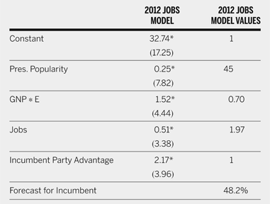
In sum, the Jobs Model seems theoretically and empirically strong, especially by comparison to the Core Model. What does it say for 2012? The model appears in table 1 (column 1). Observe that the fit-statistics are strong, in particular the standard error of estimate = 1.58. The measures are detailed at the bottom of table 1, and include observations through the 2008 contest. On the negative side, these indicate a president with limited popularity (45%), who presides over lackluster economic growth (0.70% non-annualized) and poor job creation (1.97%). On the positive side, Obama is in the White House, so can expect to benefit from an incumbency advantage. All together, these conditions yield a forecast of 48.2% for President Obama. (See the full estimated equation with 2012 values inserted, in table 1, column 2.) This result suggests a loss for President Obama. Does that forecast change if we offer a forecasting model with a different structure, as we do next?

Table 1

The Jobs Model Forecast, 2012

R-square = 0.95; adj. R-square = 0.93; SEE = 1.58; D-W = 1.42.

Dependent variable = presidential party share of the two-party vote.

Pres. Popularity = presidential popularity, as measured by the first Gallup Poll in July of the election year.

GNP = Gross National Product, as percentage change (non-annualized) in GNP (constant dollars) from the fourth quarter of the year prior to the election to the second quarter of the election year, data from the Survey of Current Business.

E = elected president running (scored 1) or not (scored .5).

J = jobs growth, in percentage change in jobs over the first 3.5 years of the president's term; the entries are calculated as follows: (number employed in June of the election year − number employed in January of the inauguration year)/(number employed in January of the inauguration year) × 100. The employment numbers are from the Civilian Labor Force (16 years and older), reported in the Bureau of Labor Statistics' Current Population Survey of Households (not seasonally adjusted).

Incumbent party advantage = scored 1 if the incumbent party candidate is the elected president (1956, 1972, 1980, 1984, 1992, 1996, 2004) or following a president who died in office (1948, 1964), scored 0 if the incumbent party candidate has a tolerable relationship with the previous president (1952, 1976, 1988, 2008), scored −1 if the incumbent party candidate and the president are not united (1960, 1968, 2000).

R-squared = the coefficient of multiple determination; the Adj. R-squared = the R-squared adjusted for degrees of freedom; SEE = the standard error of estimate; D-W = the Durbin-Watson test; * = statistical significance at .05 one-tail; the figures in parentheses are t-ratios; N = the 15 presidential election observations, 1952–2008.

THE PROXY MODEL

US presidential election forecasting models abound. [See the recent review in Lewis-Beck and Tien (Reference Lewis-Beck, Tien, Clements and Hendry2011).] Almost without exception these models base themselves on substantive explanations of the presidential vote. The proxy approach, however, does not depend on a substantive theoretical model. Instead, it rests on identification of a variable that empirically proxies the presidential vote. Through location of such a proxy, precise prediction of that vote share becomes possible. Proxy variables are standard econometric fare (Kennedy Reference Kennedy2008, 3). If a variable is unobservable, as is a future election outcome, then a proxy for it may be sought. For the proxy to be a good one, it must correlate highly with the unobserved variable. In a forecasting context, that means the proxy must approach empirical redundancy with the variable proxied. One example of a proxy model in presidential forecasting comes from the French case (Lewis-Beck, Bélanger, and Nadeau Reference Lewis-Beck, Bélanger and Nadeau2010). Here, we use a Proxy Model to forecast the US presidential election outcome.

Our proxy notion expresses itself in the following equation,

where Vote = the two-party popular presidential vote share; Vote Proxy = an observed indicator of the unobserved vote. We offer as a proxy the National Business Index (NBI), yielding

where NBI = the percentage of respondents who say “business conditions are better” minus the percentage of respondents who say “business conditions are worse,” as measured in the national University of Michigan Survey of Consumers. This variable shows itself to be quite sensitive to actual US business conditions. For example, in April of the Great Recession year of 2008, it achieves its maximum negative value over the series, at −81 (meaning respondents overwhelmingly see worse business conditions). At the other extreme is its maximum positive value, at +47, registering the prosperous year of 1984.

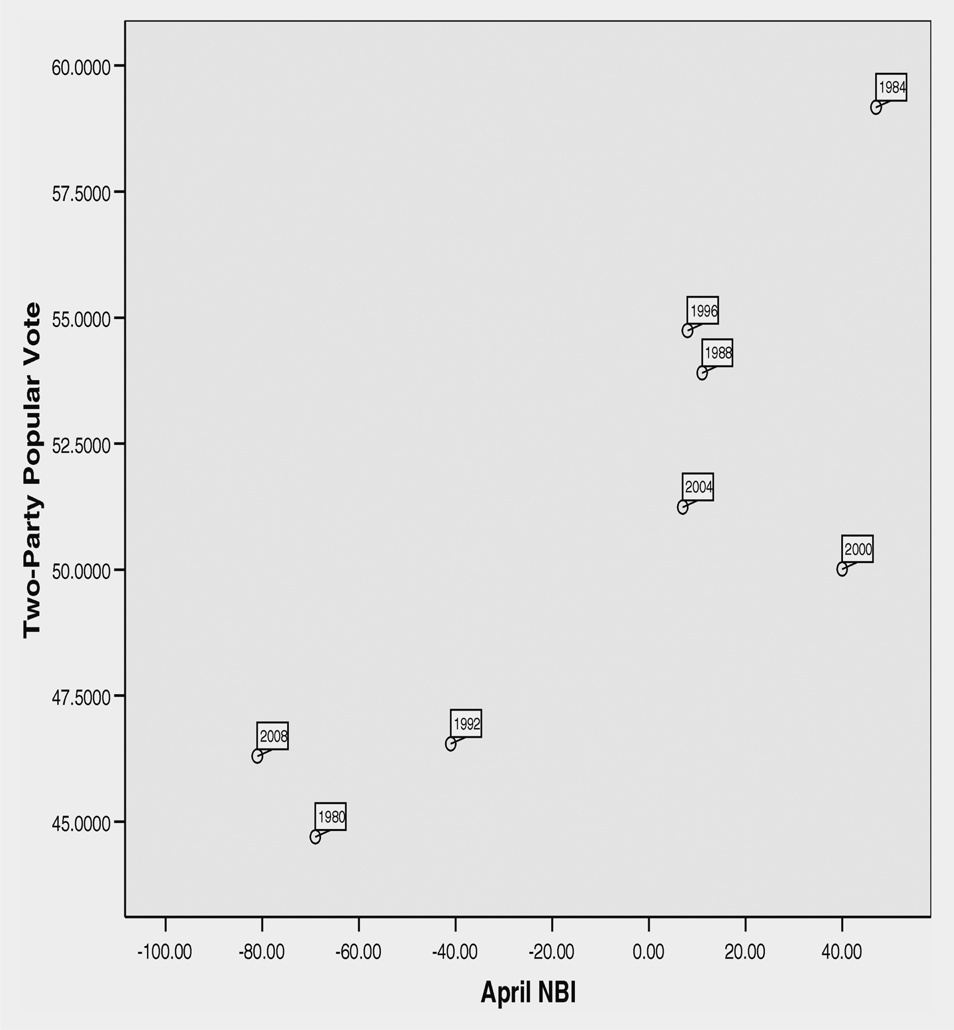
This NBI, measured in April six months before the November election, correlates highly with incumbent vote share, r = .83. Figure 1 shows this strong link, in a scatterplot over the election sample, 1980–2008. From a forecasting perspective, the six-month lead time offers considerable advantage. First, its high accuracy comes at an impressive distance from the election itself, far from the trivialities that day-before (or month-before) forecasts offer. Moreover, this longer lead performs better empirically than the commonly used three-month lag (r = .70). The strength of the six-month lead comes as no surprise. Other forecasting work, in the US, UK, and France, suggests it is optimal (Gibson and Lewis-Beck Reference Gibson and Lewis-Beck2011; Lewis-Beck and Rice Reference Lewis-Beck and Rice1992; Lewis-Beck, Bélanger, and Nadeau Reference Lewis-Beck, Bélanger and Nadeau2010).

Figure 1

Two-Party Popular Vote and April NBI, 1980–2008

The regression estimation (ordinary least squares) of this Proxy Model yields the following:

where the variables are defined as with eq. 2; the asterisk indicates statistical significance at .05, two-tail; the figures in parentheses are t-ratios; the R-squared = the coefficient of multiple determination; the Adj. R-squared = the R-squared adjusted for degrees of freedom; SEE = the standard error of estimate; D-W = the Durbin-Watson test; n = 8 observations on US presidential elections 1980–2008.

The Proxy Model of eq. 3 has promising properties. In addition to the fit statistics (of the R-squared, the Adjusted R-squared, and the SEE), it is worth examining the error produced from predicting the individual elections under study. Here are these within sample errors: 1980 = −1.06, 1984 = 3.49, 1988 = 1.33, 1992 = −1.61, 1996 = 2.39; 2000 = −5.08; 2004 = −1.02; 2008 = 1.56. Note that the most extreme NBI year, 2008 = −81, is still predicted with little error (less than 2 points). Further, we see that, with the exception of 2000, the winning party is correctly predicted, although one could argue that the 2000 popular vote winner was correctly predicted. Moreover, the exceptional case itself encourages acceptance of the model, because virtually all forecasting efforts for the Gore-Bush contest were far off (Lewis-Beck and Tien Reference Lewis-Beck and Tien2001b). In addition, a healthy distribution of residuals can be observed, with four positive and four negative signs. Overall, we see the mean absolute error (MAE) is only about 2.19 points. And, if the series is trimmed, by removing the curious 2000 case, the MAE falls to 1.78 points. These results suggest that the model can pick the winner in all but the closest races.

A final diagnostic is that its fit could not be improved, despite the addition of other obvious variables, that is, incumbency and presidential popularity, at different lags. In particular, note that presidential popularity fails to add significantly to the model because of its high collinearity with NBI, e.g., r = .85 in October. The interesting implication is that the effects of popularity are absorbed by NBI. Also, the effects of the macro-economy appear transmitted by NBI, for example, for the correlation of NBI and GNP growth, r = .68, in October. [Nadeau and Lewis-Beck (Reference Nadeau and Lewis-Beck2001), show that NBI outperforms standard macro-economic measures in predicting presidential vote support.] One implication is that the strong correlation between presidential vote share and NBI is far from spurious. Instead, NBI succeeds in empirically capturing fundamentals that operate on voters, such as presidential popularity and the macroeconomy.

NOWCASTING

Current election forecasting models share two aspects of the all-important time dimension. First, these issue unconditional forecasts months before the election. In other words, they are true forecasts. Second, these almost all offer only one unconditional forecast, typically two or three months before the election. In other words, these forecasts put all their eggs in one basket. This approach has scientific merit, resting on the assumption that the proper model specification is fixed, with a specific lag structure. However, taken literally that means “preliminary” forecasts from the model (from an earlier period) are of no value. This problem, of what might be called the “one-shot cannon,” carries special frustration for the media, who routinely ask the forecaster “What does your model say?” only to be told “too early to say” or “same as when you asked me last time.” Nowcasting offers a solution effectively making the model a “multiple-shot cannon,” with public forecast releases occurring regularly.

An election “nowcast” predicts what would happen if the election were held “now.” [We developed this nowcasting idea earlier in the forecasting of British, then French, elections. See Lewis-Beck, Nadeau, and Bélanger (Reference Lewis-Beck, Bélanger and Nadeau2010, Reference Lewis-Beck, Nadeau and Bélanger2011).] Thus, the nowcast acts as an invaluable early warning device, signaling what will come to pass unless things change. The nowcast comes from the statistical forecasting model, whose parameter estimates are held valid across current moments. That is, the model (with its fixed constant and slope values) predicts the election outcome based on current (changing) X values, as the final contest approaches. Nowcasting, then, is dynamic, and election predictions may be issued on a quarterly, monthly, or even daily basis with updates until the actual election. We have applied a nowcasting strategy to our Proxy Model, on a monthly basis, since November 2011. (See the Monkey Cage blog, where these nowcasts regularly appear.)

NOWCASTS FROM THE PROXY MODEL

The Proxy Model has several desirable properties as a forecasting equation: complete parsimony, long lead time, ease of replication, and good model fit (Lewis-Beck Reference Lewis-Beck2005). In nowcasting, we simply apply the Proxy Model as if the election were upon us—this month, or next month, or the month after—generating a series of nowcasts stretching to the actual election. To illustrate, let us use the Proxy Model to generate a nowcast, assuming the current month is November 2011, as mentioned above. Then, the equation estimates the (November 2011) election outcome from the NBI six months before (April 2011), as follows:

On the basis of the nowcasts around the turn of the year, President Obama looked like a winner, although the margin of victory was quite small. Over the initial three months of nowcasting (November, December, and January) opinion changed little, with Americans almost evenly divided on whether the economy is getting worse or better. To that point, the economy appeared “just good enough” to put Obama back in office. These results provided an early warning signal to Republicans, implying that unless things changed they will not occupy the White House this coming fall. Of course, things did change, as our subsequent nowcasts show. In table 2, we see that beginning in February the tide turned against Obama. Since that time our nowcasts put him in the losing column, until the July nowcast, which put him at 50.2% share of the two-major-party popular vote. The October and November nowcasts had Obama with 53.0% and 52.7% percent, respectively.

Table 2

The Proxy Model, Nowcasting the 2012 US Presidential Election

* Data from Survey of Consumers, University of Michigan, Table 12: Current Business Conditions Compared to a Year Ago. The question was: Would you say that at the present time business conditions are better or worse than they were a year ago?

** NBI is percent who answered better minus percent who answered worse.

*** Nowcast was calculated from following equation:

Incumbent Party Popular Vote_{current month} = 51.67 + .09 NBI_t−6

THE VOTES-TO-STATES EQUATION

In forecasting the election we observed different estimates, depending on the model chosen (see tables 1 and 2). Our standard Jobs Model issues a losing popular vote forecast (48.2%) for President Obama. However, beginning with the July nowcast from the Proxy Model Obama shows a majority. By November, the final Proxy Model nowcast gives Obama 52.7%. In sum, according to these forecasts, the popular vote will be close, with a possible win for Obama. Of course, these popular vote forecasts ignore what ultimately counts—the electoral vote. As we observed some time ago, in the modern US presidency these two measures are tightly linked, r = .96 (Lewis-Beck and Rice Reference Lewis-Beck and Rice1992, 24). Indeed, currently it is even a bit stronger, r = .97.

This tells us that popular vote share should predict electoral vote share well, as it does:

Using this regression equation, we can predict the electoral vote share. We observe that virtually any popular vote prediction under 51% generates a losing electoral vote prediction for Obama. For example, if Obama is predicted at 50.9%, then the predicted electoral vote share = 49.8% (268 electoral votes).

Such a result (less than 51%) for Obama would be poignant, since “votes-to-states” ratio, as we call it, forecasts a popular vote win and an electoral vote loss. In other words: the Gore result. Under this scenario, Obama would fall into the “win-lose triangle” or an “undemocratic window” that we earlier identified (Lewis-Beck and Tien Reference Lewis-Beck and Tien2004). That is, the small triangle in the bivariate regression scatterplot formed by the coordinates (x = 50, y = 49) and (x = 51, y = 50), where x = the popular vote share (%) and y = the electoral vote share (%). In this unique unlucky region, a presidential candidate “wins” the people but “loses” the country. (Fortunately for the function of our democracy, candidates almost never fall into this triangle. But perhaps, as some electoral rules critics would say, “almost never” is not enough.)