




No CrossRef data available.
FINITE-SAMPLE INSTRUMENTAL VARIABLES INFERENCE USING AN ASYMPTOTICALLY PIVOTAL STATISTIC
Published online by Cambridge University Press: 04 August 2003
Abstract
We consider the K-statistic, Kleibergen's (2002, Econometrica 70, 1781–1803) adaptation of the Anderson–Rubin (AR) statistic in instrumental variables regression. Whereas Kleibergen (2002) especially analyzes the asymptotic behavior of the statistic, we focus on finite-sample properties in a Gaussian framework. The AR statistic then has an F-distribution. The finite-sample distribution of the K-statistic is, however, affected by nuisance parameters. We consider two extreme cases for the nuisance parameters, which provide tight bounds for the exact distribution. The first case amounts to perfect identification—which is similar to the asymptotic case—where the statistic has an F-distribution. In the other extreme case there is total underidentification. For the latter case we show how to compute the exact distribution. We thus provide tight bounds for exact confidence sets based on the K-statistic. Asymptotically the two bounds converge, except when there is a large number of redundant instruments.The authors' research documented in this paper has been funded by the NWO Vernieuwingsimpuls research grant “Empirical Comparison of Economic Models.”
Information
- Type
- Research Article
- Information
- Copyright
- © 2003 Cambridge University Press
1. INTRODUCTION
Instrumental variables inference can be affected rather strongly by the quality of the instruments. Especially in the presence of weak instruments usual inferential procedures such as likelihood-based Wald, likelihood ratio, and Lagrange multiplier tests may show considerable size distortions, and the performance of confidence sets may be abysmally poor (see, e.g., Nelson and Startz, 1990; Staiger and Stock, 1997; Zivot, Startz, and Nelson, 1998; Hausman and Hahn, 1999). However, an exact test in a Gaussian context has been provided by Anderson and Rubin (1949). The resulting Anderson–Rubin (AR) statistic is pivotal and has an F-distribution, which does not depend on nuisance parameters and is not affected by the degree of underidentification.
However, the AR statistic has a limiting chi-square distribution with a number of degrees of freedom that equals the number of instruments. This number exceeds, or equals, the number of structural parameters, which affects the power of the test statistic. As has been shown by Kleibergen (2002) it is possible to construct a statistic, the K-statistic, with similar asymptotic pivotal properties but with a limiting chi-square distribution that has a number of degrees of freedom equal to the number of structural parameters. Thus, the K-statistic has an asymptotic distribution with a minimal number of degrees of freedom without being hampered by a poor performance close to points of underidentification, as is the case for the more traditional inference procedures. This conclusion can be drawn with respect to the asymptotic behavior of the test statistic. Kleibergen (2002) does not provide finite-sample evidence. Here we do consider finite-sample properties.
Under Gaussianity the AR statistic has an F-distribution and thus provides an exact finite-sample test. The K-statistic has a finite-sample distribution that depends on nuisance parameters. It thus does not provide an exact test. Based on the asymptotic pivotal behavior, we, however, expect the asymptotic distribution to provide an accurate approximation of the exact finite-sample distribution, but we do not know the degree of accuracy. Therefore, we compute bounds for the exact distribution of the K-statistic by assuming Gaussian distributions for the disturbances.
We find on one extreme—provided by the case of perfect identification—an F-distribution, similar to the distribution of the AR statistic, albeit with fewer degrees of freedom. On the other extreme—provided by the case of total underidentification—we find a distribution that is complicated analytically but can be simulated easily. That is, both extreme distributions can be computed in practice. We show that these extreme cases provide tight bounds. In many practical cases the two bounds are very close indeed, as we might expect based on the asymptotic pivotal property of the statistic. However, in the case of many redundant instruments, the bounds may differ even asymptotically. In fact, we also compute the limiting distribution in this case by means of the many-instruments asymptotics as described in Bekker (1994). We find it to be different from the large-sample chi-square distribution.
The paper is organized as follows. In Section 2 we describe the model and discuss the AR statistic. The K-statistic is briefly discussed in Section 3 alongside the construction of its bounding distributions. Section 4 provides some Monte Carlo computations.
2. THE MODEL AND THE ANDERSON–RUBIN STATISTIC
Consider a classical instrumental variables regression model in a cross-section context. That is, let

where Z is an n × k matrix of full column rank that consists of the nonstochastic instrumental variables and X is n × m, which may contain endogenous in addition to exogenous explanatory variables. The latter are assumed to be columns of Z also and m ≤ k. If interest is restricted to those elements of the parameter vector β that relate to the endogenous explanatory variables, the instruments in Z might be separated into two parts. For ease of exposition we will not do this and consider the m-vector β as a whole. We assume the rows of (ε,V) to be independently normally distributed with zero mean; we denote the covariance matrix by Σ.
Let in general for a matrix H of full column rank the projection matrix be denoted by PH = H(H′H)−1H′. Consider the quantity

Minimizing AR(β) over β provides the limited information maximum likelihood estimator. However, we are not concerned with estimation but with testing. If the argument in (2) equals the true β, then y − Xβ = ε and the numerator and denominator of (2) have independent chi-square distributions with k and n − k degrees of freedom, respectively. So, when multiplied by (n − k)/k, AR(β) has an Fk,n−k distribution. An exact test of H0: β = β[starf ] is found by verifying whether or not AR(β[starf ]) has a small enough p-value in the Fk,n−k distribution. The resulting test is exact and known from Anderson and Rubin (1949). Notice that the AR-statistic has an F-distribution whether or not the model is identified. That is, even if Π has a deficient column rank AR(β) will be distributed as an Fk,n−k random variable. This shows that it is a pivotal statistic.
Although the AR-test is exact under Gaussianity, it may have poor power if the number of instruments k exceeds the number of explanatory variables m. That is, in the numerator of (2), y − Xβ is projected on the full space spanned by Z. We know, however, that, if β deviates from the true value, the mean of y − Xβ is located in the subspace spanned by ZΠ. The problem is then that we do not know Π. Still, the dimension of the space onto which we project y − Xβ can be reduced in a way that preserves the pivotal property of the statistic asymptotically.
3. BOUNDING THE EXACT DISTRIBUTION OF THE K-STATISTIC
Consider a regression of the columns of V on ε. That is, let

where W is independent of ε and where σV,ε and σε2 denote the covariance of V and ε and the variance of the latter, respectively. Consequently, X − ελ′ = ZΠ + W is like Z independent of ε but has a smaller column dimension. If λ were known, we could replace the projection matrix PZ in the numerator of (2) by

, with

For the true value of β,

is stochastically independent of ε. Thus, this adaptation of the AR statistic would still be pivotal but now distributed, when multiplied by (n − k)/m, as Fm,n−k. Of course, λ is unknown. However, Kleibergen (2002) simply uses a consistent estimator of λ that is stochastically independent of Z′y and Z′X under the null where β is specified. This estimator,

, is specified as in (3) with σV,ε and σε2 replaced by

The resulting K-statistic is given by

Asymptotically, it is distributed as a chi square with m degrees of freedom. Further discussions are given by Kleibergen (2002).
The denominator of the K-statistic (6) is given by

, so it results from projecting the first column of the following matrix onto the space that is spanned by its last m columns:

Theorem 1 states an alternative expression of the K-statistic that results from (7).
THEOREM 1. An alternative expression of the K-statistic (6) is

where the matrix

is defined by

with W as in (3) and

Proof. See the Appendix.
If the matrix ΠΣ−1/2 from Theorem 1 were known, the distribution of K(β) could be simulated, because

can be simulated, as their elements are independent standard normal distributed. However, the matrix ΠΣW−1/2 is not known. Still we can distinguish between two extreme cases.
THEOREM 2. When Π = θΠ[starf ], where Π[starf ] is a fixed finite k × m matrix and θ is a scalar, K(β) is a stochastically decreasing function of |θ|, so its finite-sample distribution moves to the left when |θ| increases. Hence, the finite-sample distribution of K(β) is bounded from above by the distribution that results in the case of a zero value of θ and from below by the distribution that results in the case of an infinite value of |θ|.
Proof. See the Appendix.
The bounds on the finite-sample distribution of K(β) in Theorem 2 result from extremal values of the nuisance parameters in the expression of the exact finite-sample distribution of K(β). Hence, they do not result from bounding the statistic of interest directly as, for example, in Sargan and Bhargava (1983). Sargan and Bhargava (1983) obtain upper and lower bounds on the distribution of their statistic of interest by constructing lower and upper bounds of the statistic itself using properties of ratios of quadratic forms. We obtain the bounds in an entirely different manner and construct them from the finite-sample distribution.
The upper bound on the finite-sample distribution of K(β) results from the extreme case of total underidentification: Π = 0. In this case the distribution can be simulated easily. The distribution depends only on the dimension parameters k, m, and n. In the case of an infinite value of θ, which forms the lower bound on the finite-sample distribution of K(β),

converges in probability to PZΠ, and so the distribution of K(β)/m converges to Fm,n−k.
The preceding discussion implies that we can compute bounds for the finite-sample distribution of the K-statistic using simulation. Conservative tests or confidence sets can be based on the critical value found for the distribution simulated at Π = 0. However, if n is large then

is small, in probability, and the correlation between

becomes negligible. In that case the bounds are very close. Indeed, if n → ∞, then

(see Kleibergen, 2002).
Would this limit distribution also provide an accurate approximation if there are many redundant instruments? To answer this question we consider the limit distribution of K(β) for an asymptotic parameter sequence where the number of instruments increases with the number of observations: k/n → α > 0.
For the lower bound we found a finite-sample distribution given by Fm,n−k. Clearly, the lower bound converges to a χm2-distribution whether or not α > 0. For the upper bound, where Π = 0, the results are summarized in Theorem 3.
THEOREM 3. The limiting distribution of the K-statistic when Π = 0 and k/n → α > 0 is characterized by

Proof. See the Appendix.
If α > 0 we thus find a simple difference between the asymptotic upper and lower bounds. The difference is of order k/n. These practical results are confirmed numerically in the next section.
4. MONTE CARLO RESULTS
To determine the applicability of the bounds on the exact distribution of K(β), we construct the bounds for m = 1 and some values of k and n. Figures 1 and 2 show the lower and upper bounds on the exact distribution function of K(β)/m. Figure 2 shows that there is a considerable difference between the lower and upper bounds when k/n is large. Figure 1 shows that when k/n gets smaller, the difference decreases and becomes negligible, as expected. The figures also contain a limiting approximation of the upper bound. Instead of the asymptotic approximation χm2/m, based on (15), we used the Fm,n−k distribution, which is more accurate in small samples and more convenient too, because it is also used for the lower bound. The figures show that this limiting approximation is accurate even for small values of n. Hence, it suffices to use critical values from the Fm,n−k distribution both as lower bound and, by multiplying them by 1/(1 − k/n), as upper bound of the exact critical values of K(β)/m.

Lower bound (—) and upper bound (- -) and limiting approximation of upper bound (…) of the distribution function of K(β)/m for n = 25, k = 5, and m = 1.

Lower bound (—) and upper bound (- -) and limiting approximation of upper bound (…) of the distribution function of K(β)/m for n = 25, k = 10, and m = 1.
APPENDIX
Proof of Theorem 1. The second term in (7) can be expressed as

where the last equality follows from

Consequently, the K-statistic K(β) is given by

Proof of Theorem 2. To prove that K(β) is stochastically decreasing in |θ|, where Π = θΠ[starf ], we first condition on

. This does not affect the distribution of

. Let

We may regress u on U so that u = Uγ + ν, where ν is independent of U. Next we also condition on U and consider the numerator of K(β) given by

Let Q be an orthogonal m × m dimensional matrix such that Uγ is orthogonal to the last m − 1 columns of L(L′L)−1/2Q, such that it has a positive inner product with the first column: (γ′U′PLUγ)1/2. Furthermore let ξ = Q′(L′L)−1/2L′ν, whose elements are independently normally distributed; then

Consequently, we only have to show that, conditional on U, (ξ1 + (γ′U′PLUγ)1/2)2 stochastically decreases as |θ| increases. Here we find an analogy with the noncentral χ2 distribution that decreases as the noncentrality parameter decreases. So we only have to prove that the nonrandom function

decreases as |θ| increases. This can be shown to hold true by considering the derivative with respect to θ, which completes the proof. █
Proof of Theorem 3. We use the following limits, which can be easily verified:

so

Furthermore,

so

Consequently,

References
REFERENCES
Anderson, T.W. &
H. Rubin
(1949)
Estimators on the parameters of a single equation in a complete set
of stochastic equations.
Annals of Mathematical Statistics
21,
570–582.Google Scholar
Bekker, P.A.
(1994)
Alternative approximations to the distributions of instrumental
variable estimators.
Econometrica
62,
657–681.Google Scholar
Hausman, J. &
J. Hahn
(1999)
A New Specification Test for the Validity of Instrumental
Variables.
Working paper,
Massachusetts Institute of Technology.
Kleibergen, F.
(2002)
Pivotal statistics for testing structural parameters in
instrumental variables regression.
Econometrica
70,
1781–1803.Google Scholar
Nelson, C.R. &
R. Startz
(1990)
Some further results on the exact small sample properties of the
instrumental variables estimator.
Econometrica
58,
967–976.Google Scholar
Sargan, J.D. &
A. Bhargava
(1983)
Testing residuals from least squares regression for being generated
by the Gaussian random walk.
Econometrica
51,
153–174.Google Scholar
Staiger, D. &
J.H. Stock
(1997)
Instrumental variables regression with weak instruments.
Econometrica
65,
557–586.Google Scholar
Zivot, E.,
R. Startz, &
C.R. Nelson
(1998)
Valid confidence intervals and inference in the presence of weak
instruments.
International Economic Review
39,
1119–1144.Google Scholar
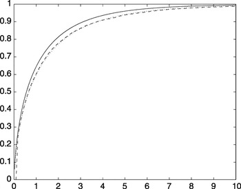
Lower bound (—) and upper bound (- -) and limiting approximation of upper bound (…) of the distribution function of K(β)/m for n = 25, k = 5, and m = 1.
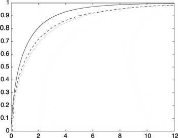
Lower bound (—) and upper bound (- -) and limiting approximation of upper bound (…) of the distribution function of K(β)/m for n = 25, k = 10, and m = 1.
 You have
Access
- 11
- Cited by