


1 Introduction
Let U be a smooth scheme of finite type over k a subfield of
$\mathbb {C}$
 , and
$x,y$
 be rational points on U. Denote by
$\pi _1^{\mathrm {un}}(U(\mathbb {C}),x,y)$
 the prounipotent completion of the fundamental torsor of
$U(\mathbb {C})$
 at
$x,y$
 . P. Deligne conjectured in [Reference DeligneDel89] the existence of a motivic incarnation of
$\pi _1^{\mathrm {un}}(U(\mathbb {C}),x,y)$
 , and in joint work with A. B. Goncharov, he showed in [Reference Deligne and GoncharovDG05, Subsection 3.12] that
$\mathcal {O}(\pi _1^{\mathrm {un}}(U(\mathbb {C}),x,y))$
 arises as the degree-zero homology of the Betti realization of an algebra object in Voevodsky’s triangulated category of mixed motives called the motivic pointed path space of
$\mathbf {U}$
 based at
$\mathbf {x,y}$
 . In the presence of a motivic t-structure (for instance if U is of mixed Tate type over a field satisfying Beilinson–Soulé’s conjecture), this construction yields the motivic fundamental torsor
$\pi _1^m(U,x,y)$
 whose Betti realization is
$\pi _1^{\mathrm {un}}(U(\mathbb {C}),x,y)$
 .
However, many interesting varieties have no rational points, or more generally no section over their base scheme, as is the case for the moduli spaces of curves of genus g with n marked points
$\mathcal {M}_{g,n}$
 viewed as
$\mathbb {Z}$
 -schemes. In this situation, one must replace rational basepoints by tangential basepoints, that is, points on a smooth compactification with simple normal crossings divisor, equipped with a nonzero tangent vector normal to each component of the divisor. In certain specific cases, most notably for
$\mathcal {M}_{0,4} \simeq \mathbb {P}^1_{\mathbb {Z}}\setminus \{0,1,\infty \}$
 , Deligne and Goncharov established [Reference Deligne and GoncharovDG05, Theorem 4.4] the existence of the motivic fundamental torsor at tangential basepoints whose realizations were previously defined in [Reference DeligneDel89]. However, their proof is transcendental in nature and does not provide an explicit construction.
In this article we generalize this work by giving a construction of the motivic pointed path space based at tangential basepoints on any smooth scheme over a field endowed with a simple normal crossings divisor. More specifically, let
$\mathcal {DA}(k,\Lambda )$
 be the stable
$\infty $
 -category of motives over a field k with
$\Lambda $
 coefficients as defined by J. Ayoub [Reference Ayoub, Gallauer and VezzaniAGV22], D.-C. Cisinski and F. Déglise [Reference Cisinski and DégliseCD19] and others, and
$\mathrm {R}_{\mathrm {B}},\mathrm {R}_{\mathrm {dR}}$
 its Betti and de Rham realization functors (with
$\Lambda = \mathbb {Q},\; k \subset \mathbb {C}$
 and
$\Lambda = k, \; k$
 of characteristic
$0$
 respectively). The main theorem we will prove is the following:
Theorem 1.0.1 (Definition 4.2.1 Theorems 5.2.11, 5.3.6, 5.5.10)
Let X be a smooth scheme of finite type over an arbitrary field k, endowed with a simple normal crossings divisor D and let
$\mathbf {x},\mathbf {y}$
 be tangential basepoints for the pair
$(X,D)$
 (definition 2.1.1).
-
• We construct a commutative algebra object $\displaystyle \,_{\mathbf {x}}^{}\mathrm {P}^m_{\mathbf {y}} (X\setminus D) \in \mathcal {DA}(k,\Lambda )$
 , the motivic pointed path space of
$\mathbf {X\setminus D}$
based at
$\mathbf {x},\mathbf {y}$
, such that the family
$\{\mkern1mu_{\mathbf {x}}^{}\mathrm {P}^m_{\mathbf {y}} (X\setminus D)\}_{\mathbf {x},\mathbf {y}}$
has the structure dual to that of a groupoid, in the sense of theorem 4.1.9.
-
• If $k \subset \mathbb {C}$
and
$\Lambda = \mathbb {Q}$
, its Betti realization satisfies $$ \begin{align*} \mathrm{H}^0(\mathrm{R}_{\mathrm{B}}\mkern1mu_{\mathbf{x}}^{}\mathrm{P}^m_{\mathbf{y}}(X\setminus D)) \simeq \mathcal{O}(\pi_1^{\mathrm{un}}(X(\mathbb{C})\setminus D(\mathbb{C}),\mathbf{x},\mathbf{y})) \end{align*} $$which is the prounipotent completion of the fundamental torsor of $X(\mathbb {C})\setminus D(\mathbb {C})$
at
$\mathbf {x},\mathbf {y}$
in the sense of definition 5.2.3.
-
• If k is of characteristic $0$
, and
$\Lambda = k$
, its de Rham realization is described by $$ \begin{align*}\mathrm{R}_{\mathrm{dR}}\mkern1mu_{\mathbf{x}}^{}\mathrm{P}^m_{\mathbf{y}}(X\setminus D) \simeq \mkern1mu_{\mathbf{x}}\mathrm{Bar}_{\mathbf{y}}\mathbf{R}\Gamma\big(X,\Omega_{X/k}(\mathrm{log}D)\big),\end{align*} $$the bar construction on the logarithmic de Rham complex of $(X,D)$
pointed at
$\mathbf {x},\mathbf {y}$
in the sense of definition 5.3.1.
-
• The periods associated with the comparison isomorphism
(1) $$ \begin{align} \mathrm{H}^0(\mathrm{R}_{\mathrm{B}}\mkern1mu_{\mathbf{x}}^{}\mathrm{P}^m_{\mathbf{y}}(X\setminus D))\otimes_{\mathbb{Q}} \mathbb{C} \simeq \mathrm{H}^0(\mathrm{R}_{\mathrm{dR}}\mkern1mu_{\mathbf{x}}^{}\mathrm{P}^m_{\mathbf{y}}(X\setminus D)) \otimes_k \mathbb{C} \end{align} $$are given by regularized iterated integration of forms with logarithmic poles along D in the sense of definition 5.5.8.








Remark 1.0.2. The isomorphism (1) is a version with tangential basepoints of K. T. Chen’s theorem on iterated integrals [Reference ChenChe77, Theorem 2.6.1]. To the best of our knowledge, this general form is new, and the case of a curve appeared in [Reference Ignacio Burgos Gil and FresánBGF25].
In the presence of a motivic t-structure, the motivic fundamental torsor of
$\mathbf {X\setminus D}$
 at
$\mathbf {x},\mathbf {y}$
 is defined by:

the affine scheme associated with the algebra
$\mathrm {H}_{\mathrm {mot}}^0(\mkern1mu_{\mathbf {x}}^{}\mathrm {P}^m_{\mathbf {y}}(X\setminus D))$
 , where the functor
$\mathrm {H}^0_{\mathrm {mot}}$
 is the
$0$
 -truncation functor associated with the motivic t-structure.
We remind the reader that such a t-structure exists for mixed Tate motives, when k satisfies Beilinson–Soulé’s conjecture, which is known when k is a finite field, a number field, a field of rational functions on a curve of genus
$0$
 over a number field, and filtered colimits of such fields [Reference Deligne and GoncharovDG05, 1.6].
Remark 1.0.3. If we take
$(X,D) = (\mathbb {P}^1_{\mathbb {Q}},\{0,1,\infty \})$
 and
$\mathbf {x},\mathbf {y}$
 any tangential basepoints, this gives a complete definition of
$\pi _1^m(\mathbb {P}^1_{\mathbb {Q}}\setminus \{0,1,\infty \},\mathbf {x},\mathbf {y})$
 in the category of mixed Tate motives over
$\mathbb {Q}$
 . When
$\mathbf {x},\mathbf {y} \in \{(0,\pm \frac {\partial }{\partial z}\big |_0),(1,\pm \frac {\partial }{\partial z}\big |_1),(\infty ,\pm \frac {\partial }{\partial z^{-1}}\big |_\infty )\}$
 with z the standard coordinate around
$0$
 , it is natural from the definition to view this object in the category of mixed Tate motives over
$\mathbb {Z}$
 . In general, we hope that our results can be generalized over any base scheme.
Another definition of the motivic fundamental torsor at tangential basepoints can be found in M. Levine’s [Reference LevineLev07] in the case of curves of mixed Tate type via his definition of motivic tubular neighbourhoods. We expect this construction to be equivalent to ours.
At the same level of generality as our theorem 1.0.1, Hain proved in [Reference HainHai87b] the existence of an ind-Hodge structure on
$\mathcal {O}(\pi _1^{\mathrm {un}}(X(\mathbb {C})\setminus D(\mathbb {C}),\mathbf {x}))$
 , unconditionally by obtaining it as a limit Hodge structure after degenerating a family of ordinary rational points of
$X\setminus D$
 into the tangential basepoint
$\mathbf {x}$
 . Although we do not compute the Hodge realization of the motivic pointed path space of
$X\setminus D$
 at
$\mathbf {x}$
 , we hope that it coincides with Hain’s, thus extending in a natural way his construction for ordinary basepoints [Reference HainHai87a].
1.1 The case of ordinary basepoints
Let us recall the classical construction of the motivic fundamental group (we restrict to a single basepoint to simplify). For U a smooth scheme of finite type over a field k, and
$x \in U(k)$
 , Z. J. Wojtkowiak [Reference WojtkowiakWoj93] defines the cosimplicial loop space at x, defined by analogy with classical topology as the pullback of cosimplicial schemes

Deligne and Goncharov define the motivic pointed path space of U at x, denoted by
$\mkern1mu^{}_x\mathrm {P}^m_xU$
 , as the motivic complex associated with the simplicial motive
$h(\mkern1mu^{}_x\mathrm {P}^{\bullet }_xU)$
 , with h the cohomological motive functor. It is isomorphic to the bar construction of the commutative algebra object
$h(U)$
 augmented by the point
$h(x) : h(U) \xrightarrow {}~h(*)$
 . When U is of mixed Tate type over a field satisfying Beilinson–Soulé’s conjecture, the motivic fundamental group is defined by

Its Betti realization is identified via Beilinson’s theorem [Reference GoncharovGon01, Theorem 4.1][Reference Deligne and GoncharovDG05, Proposition 3.4] which shows that when
$k \subset \mathbb {C}$
 there is a natural isomorphism of Hopf algebras over
$\mathbb {Q}$


where I is the kernel of the map
$\mathbb {Q}[\pi _1(U(\mathbb {C}),x)] \rightarrow \mathbb {Q}$
 sending every element of the fundamental group to
$1$
 , and where the left cohomology group is computed by taking the cohomology of the double complex induced by the cosimplicial structure.
Its de Rham realization is described by the bar construction [Reference Esnault and LevineEL11, Section 1.2] on the augmented (by evaluation at x) commutative differential graded algebra of regular differential forms on U denoted by
$\Omega _{U/k}$
 when k is of characteristic
$0$
 . If we suppose U to be affine to simplify, then there is a canonical isomorphism of Hopf algebras over k

where
$\mkern1mu_x \mathrm {Bar}_x(\Omega _{U/k}(U))$
 is the differential graded Hopf algebra whose elements are denoted by

The Betti–de Rham comparison theorem for the motivic fundamental group is then obtained via K. T. Chen’s theorem [Reference ChenChe77, Theorem 2.6.1] which states that there is a natural isomorphism of Hopf algebras over
$\mathbb {C}$
 :

Every class in
$\mathrm {H}^0\big (\mkern1mu_x \mathrm {Bar}_x(\Omega _{U/k}(U))\big )\otimes _k \mathbb {C}$
 is represented by elements
$[\omega _1|\dots |\omega _k]$
 where
$\omega _i$
 is a
$1$
 -form [Reference Ignacio Burgos Gil and FresánBGF25, Lemma 3.263], and the pairing underlying this theorem is induced by the iterated integration of
$1$
 -forms

where
$\gamma $
 is a smooth loop on U based at x.
1.2 The case of tangential basepoints
In the case of a tangential basepoint
$\mathbf {x}$
 on X a smooth scheme of finite type over k endowed with a simple normal crossings divisor D, this method fails overall. Indeed, since
$\mathbf {x}$
 cannot be defined by a geometric morphism
$* \rightarrow X\setminus D$
 , it is impossible a priori to define the cosimplicial path space based at
$\mathbf {x}$
 , or the augmentation on
$\Omega _{X(\mathbb {C})\setminus D(\mathbb {C})}$
 associated with
$\mathbf {x}$
 in such a straightforward way.
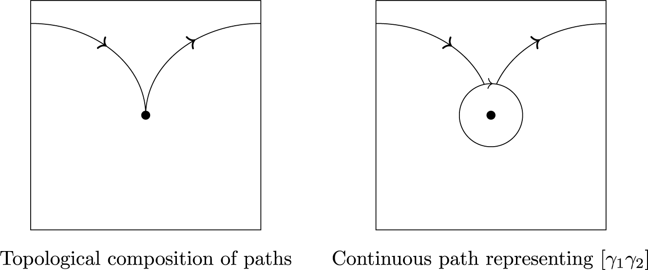
In the topological setting, Deligne explains in [Reference DeligneDel89] how tangential basepoints can be viewed as ordinary points. For instance, for X a smooth curve over
$k \subset \mathbb {C}$
 endowed with
$D := \{x\}$
 and
$\mathbf {x} := (x,v)$
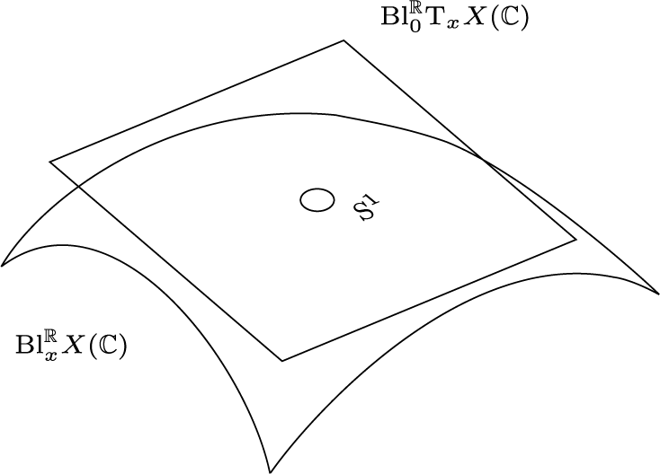
 a tangential basepoint at x, let
$X'$
 be the gluing of
$\mathrm {Bl}_x^{\mathbb {R}}X(\mathbb {C})$
 the real-oriented blow-up of
$X(\mathbb {C})$
 at x with
$\mathrm {Bl}_0^{\mathbb {R}}\mathrm {T}_xX(\mathbb {C})$
 the real-oriented blow-up of the tangent space at
$0$
 along the infinitesimal unit circles. The picture representing this construction is:
The topological space
$X'$
 has the homotopy type of
$X(\mathbb {C})\setminus D(\mathbb {C})$
 , so Deligne defines the fundamental group of
$X(\mathbb {C})\setminus D(\mathbb {C})$
 at
$\mathbf {x}$
 as

where the tangential basepoint
$\mathbf {x}$
 is viewed as the point

This point of view, as well as similar approaches in the étale and crystalline contexts, allows Deligne to construct the expected realizations of the motivic fundamental group at a tangential basepoint in [Reference DeligneDel89].
1.3 Content of the paper
Our construction is inspired by Deligne’s Betti picture (Figure 1) for tangential basepoints, and it allows us to apply the cosimplicial loop space/bar construction approach in the setting of tangential basepoints. The main tools we will use are logarithmic geometry and the theory of motives for logarithmic schemes, as developed in the recent work of F. Binda, P. A. Østvær and D. Park [Reference Binda, Park and Arne ØstværBPØ22, Reference ParkPar22, Reference Binda, Park and Arne ØstværBPØ25]. Moreover, we adopt the guiding principle that the motivic fundamental torsor should be functorial with respect to the datum
$(X,\mathbf {x},\mathbf {y})$
 . The details of this functoriality are subtle and will be described later (see definition 2.1.9).
The topological space
$X'$


Figure 1. Long description
At the center is a small circle labeled S one. This circle is enclosed by a square. The square is inscribed within a larger curved surface. The lower left of the curved surface is labeled B l superscript R sub x X open parenthesis C close parenthesis. The upper right of the square is labeled B l superscript R sub zero T sub x X open parenthesis C close parenthesis. The square and curved surface are not parallel, emphasizing their distinct geometric roles.
Logarithmic geometry, developed under the influence of J.-M. Fontaine and L. Illusie, and further formulated by K. Kato [Reference KatoKat89], is a variant of classical algebraic geometry designed to formalize the notion of ‘algebraic varieties with boundaries’. A log scheme is the datum
$(\underline {X},\mathcal {M}_X)$
 of a scheme
$\underline {X}$
 and of a sheaf of monoids (for the Zariski topology in our case)
$\mathcal {M}_X$
 endowed with a morphism of sheaves in monoids
$\alpha _X: \mathcal {M}_X \rightarrow \mathcal {O}_X$
 inducing an isomorphism
$\alpha _X^{-1}(\mathcal {O}_X^\times ) \simeq \mathcal {O}_X^\times .$
 For instance any scheme
$\underline {X}$
 is endowed with a trivial log scheme structure, i.e.
$\mathcal {M}_X:= \mathcal {O}_X^\times $
 . A classical family of examples of non-trivial log structures is given by the datum of pairs
$(\underline {X},\underline {D})$
 where
$\underline {X}$
 is a regular scheme endowed with
$\underline {D}$
 a simple normal crossings divisor, so that the log structure is given on
$\underline {X}$
 by
$\mathcal {M}_X:= j_*\mathcal {O}_{X\setminus D}^\times $
 where
$j: \underline {X}\setminus \underline {D} \hookrightarrow \underline {X}$
 . We call these log schemes divisorial log schemes [Reference OgusOgu18, III.1.6.1].
By the work of Kato and C. Nakayama in [Reference Kato and NakayamaKN99], we know that classical cohomology theories are extended to log schemes (e.g. log Betti, log de Rham, log étale cohomologies). These extensions compute the same groups as their classical counterparts when applied to a scheme with trivial log structure. The log Betti, log de Rham and log étale cohomologies with torsion coefficients prime to the characteristic of the base field, have the expected property that for
$(\underline {X},\underline {D})$
 a divisorial log scheme, the log cohomology of
$(\underline {X},\underline {D})$
 computes the classical cohomology of
$\underline {X}\setminus \underline {D}$
 (this is true for a more general class of logarithmic schemes: log smooth schemes over a field).
Specifically, for any log scheme X the log de Rham cohomology of X is computed via the log de Rham complex
$\Omega _X$
 which is nothing but the complex of forms on
$\underline {X}$
 with logarithmic poles at
$\underline {D}$
 in the case of a divisorial log scheme
$(\underline {X},\underline {D})$
 . The log Betti cohomology of X is given by the singular cohomology of the Kato–Nakayama space associated with X, which is the real-oriented blow-up of
$X(\mathbb {C})$
 along
$D(\mathbb {C})$
 in the case of
$(\underline {X},\underline {D})$
 .
These cohomology theories are encompassed within a logarithmic motivic homotopy theory. We recall this theory in detail in section 3. In particular, there is a stable
$\infty $
 -category of
$\mathbb {A}^1$
 -invariant log motives over a field k with coefficients
$\Lambda $
 denoted by
$\mathcal {DA}^{\mathrm {log}}(k,\Lambda )$
 constructed by Park [Reference ParkPar22], equivalent to the category
$\mathcal {DA}(k,\Lambda )$
 . In this category, we have the cohomological motive
$h(X)$
 of X a (fine saturated) log scheme of finite type over k.
In the category
$\mathcal {DA}^{\mathrm {log}}(k,\Lambda )$
 , there is an equivalence

(corollary 3.2.3) where
$0^{\mathrm {log}}$
 is the log scheme obtained by restricting the log structure of
$(\mathbb {A}^1,\{0\})$
 on
$0$
 . This phenomenon, when viewed in Betti realization is just a reflection of the topological retractibility of the real-oriented blow-up of
$\mathbb {C}$
 at
$0$
 on its infinitesimal unit circle, since the Kato–Nakayama space of
$0^{\mathrm {log}}$
 is
$S^1$
 . This can be related to Deligne’s trick to view tangential basepoints as ordinary points: for
$\underline {X}$
 a smooth curve over k,
$\underline {D}\subset \underline {X}$
 a finite set of closed points, and for
$x\in \underline {D}(k)$
 , let us endow
$\mathrm {T}_x\underline {X}$
 with the log scheme structure
$(\mathrm {T}_x\underline {X},\{0\})$
 . The log scheme
$0^{\mathrm {log}}$
 obtained by restriction of the log structure of
$(\mathrm {T}_x\underline {X},\{0\})$
 to
$0$
 is canonically isomorphic to the log scheme
$x^{\mathrm {log}}$
 obtained by restriction of the log structure of
$(\underline {X},\underline {D})$
 to x. Hence there is a diagram of logarithmic schemes

This diagram is a logarithmic geometric version of the figure 1. Take a tangential basepoint
$\mathbf {x} := (x,v)$
 at x. By (2), there is a sequence of morphisms

This defines an augmentation on the commutative algebra object
$h(\underline {X},\underline {D})$
 associated with
$\mathbf {x}$
 , denoted by
$h(\mathbf {x})$
 . Note in particular that the log scheme
$(\mathrm {T}_x \underline {X},\{0\})$
 has the property that the set of morphisms of log schemes

is in bijection with the set of rational points of
$\mathrm {T}_x \underline {X}\setminus \{0\}$
 i.e. with the set of tangential basepoints at x, since a morphism from the point with trivial log structure to any log scheme lands on the locus of points where the log structure is trivial.
Motivated by this example, in section 2 we define, for any divisorial log scheme
$(\underline {X},\underline {D})$
 and
$x \in \underline {X}(k)$
 , in a functorial manner, a log scheme
$\mathrm {N}_x^{\mathrm {log}}(\underline {X},\underline {D})$
 (definition 2.1.4) whose underlying scheme is isomorphic to the normal space of X to D at x and such that the set of its logarithmic rational points (i.e. morphisms of log schemes
$\mathrm {Spec}(k) \rightarrow \mathrm {N}_x^{\mathrm {log}}(\underline {X},\underline {D})$
 ) is in bijection with the set of tangential basepoints at x.
We deduce from this that the category of tangentially pointed divisorial log schemes is equivalent to the category of pointed diagrams that is the category of diagrams of the shape

Once again by a consequence of (2) (see corollary 3.2.5), each pointed diagram defines an augmentation in a functorial way; in section 3 we show that the cohomological motive functor defines a contravariant functor from the category whose objects are divisorial log schemes over k with the datum of a tangential basepoint
$(\underline {X},\underline {D},\mathbf {x})$
 to the
$\infty $
 -category
$\mathrm {CAlg}(\mathcal {DA}^{\mathrm {log}}(k,\Lambda ))^{/\Lambda }$
 (definition 3.3.5).
This allows us to define in section 4, after complements on the bar construction in an
$\infty $
 -categorical context, via theorem 4.1.9 and definition 4.2.1 the motivic pointed path space in a similar way as the case of ordinary basepoints:
Definition 1.3.1. The motivic pointed path space is defined as

We show in theorem 4.1.9 that the family
$\{\mkern1mu^{}_{\mathbf {x}}\mathrm {P}^m_{\mathbf {y}}(\underline {X}\setminus \underline {D})\}$
 is endowed with the structure of a homotopy Hopf algebroid. In particular,
$\mkern1mu^{}_{\mathbf {x}}\mathrm {P}^m_{\mathbf {x}}(\underline {X}\setminus \underline {D})$
 is a Hopf algebra for all augmentations
$\mathbf {x}$
 .
In section 5, we check that the Betti and de Rham realizations of the motivic pointed path space yield the expected theorems 1.3.2 and 1.3.3. Using the formalism of B. Drew in [Reference DrewDre18], we build the Betti and de Rham realization functors
$\mathrm {R_B},\mathrm {R_{dR}}$
 from
$\mathcal {DA}^{\mathrm {log}}(k,\mathbb {Q})$
 and
$\mathcal {DA}^{\mathrm {log}}(k,k)$
 , and we check the expected property of the Betti fundamental group.
Theorem 1.3.2 (Theorem 5.2.11)
Let
$(\underline {X},\underline {D})$
 be a divisorial log scheme and
$\mathbf {x}, \mathbf {y}$
 be tangential basepoints of
$(\underline {X},\underline {D})$
 . There is a natural equivalence of algebras

On the de Rham side, we show that the de Rham realization of the motivic pointed path space is

The augmentations needed to define the bar construction can be viewed via the interpretation of tangential basepoints as virtual morphisms, an extension of the available morphisms between log schemes (a notion defined by N. L. Howell in [Reference HowellHow17]). This interpretation developed by C. Dupont, E. Panzer and B. Pym in [Reference Dupont, Panzer and PymDPP23] is compared to the preceding in section 2. Using this comparison, and results from [Reference Dupont, Panzer and PymDPP23] we compute the Betti–de Rham comparison theorem applied to the motivic pointed path space, and compute the resulting periods:
Theorem 1.3.3 (Theorem 5.5.10)
The Betti–de Rham comparison isomorphism applied to
$\mkern1mu^{}_{\mathbf {x}}\mathrm {P}^m_{\mathbf {y}}(\underline {X}\setminus \underline {D})$
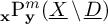 is induced by the pairing

given by

where the integral sign is the regularized iterated integral of
$\omega _1,\dots ,\omega _k$
 along
$\gamma $
 .
This generalizes Chen’s theorem to forms with log poles. When
$X = (\mathbb {P}_{\mathbb {Q}}^1,\{0,1,\infty \})$
 , this recovers the regularization of multiple zeta values described in [Reference Ignacio Burgos Gil and FresánBGF25, Section 3.8.5].
1.4 Remarks and relations with other works
Virtual logarithmic geometry was defined by N. L. Howell in [Reference HowellHow17] and later reformulated by G. Shuklin in [Reference ShuklinShu22], with already the wish to show that it is integrated in a motivic formalism. In particular, Shuklin is able to define in a functorial way the motive of a virtual logarithmic scheme in Voevodsky’s category of étale motives. It is possible to define the motivic pointed path space in this context using the correspondence between tangential basepoints and virtual points mentioned earlier. The Betti realization yields the correct object, but we do not know how to compute its de Rham realization. It is unclear if Binda, Park and Østvær’s definition of the motive of a log scheme coincide with Shuklin’s so we cannot prove that such a construction would be equivalent to ours.
Nevertheless, if a category of log motives with virtual morphisms were to be constructed, it would simplify greatly the constructions in the present article, since the construction for rational points would be transposed directly.
Notations and conventions
We follow Ogus’ reference book [Reference OgusOgu18] regarding most logarithmic geometry notations except for the Kato–Nakayama space of a log-scheme X that we denote by
$X^{\mathrm {KN}}$
 . We only consider log schemes with Zariski log structures. We denote by
$\mathbb {A}_{\mathbb {N}^r}:= (\mathbb {A}^r = \mathrm {Spec}(k[t_1,\cdots ,t_r], \{t_1\cdots t_r = 0\})$
 . We also let
$*_{\mathbb {N}^r}$
 denote the log structure of
$\mathbb {A}_{\mathbb {N}^r}$
 restricted to
$0 \in \mathbb {A}^r$
 .
To simplify the notations, we will often refer to a divisorial log scheme
$(\underline {X},\underline {D})$
 simply by ‘X’, so that although we described the motivic pointed path space as ‘
$\!^{}_{\mathbf {x}}\mathrm {P}^m_{\mathbf {y}}(\underline {X}\setminus \underline {D})$
 ’ in the introduction, we will denote it by ‘
$\!^{}_{\mathbf {x}}\mathrm {P}^m_{\mathbf {y}}X$
 ’. Note that since the motives of X and
$\underline {X}\setminus \underline {D}$
 coincide, this is consistent.
For all
$\infty $
 -categorical notations, unless specified otherwise, we refer to Lurie’s foundational articles [Reference LurieLur09] and [Reference LurieLur17]. Note that for
$\mathcal {C}$
 an
$\infty $
 -category, and X an object of
$\mathcal {C}$
 , we denote by
$\mathcal {C}^{/X}$
 (resp.
$\mathcal {C}^{//X}$
 ) the category of objects under X (resp. twice under X), that is endowed with a morphism (resp. two morphisms) from X. We will also denote by curved letters
$\mathcal {C}$
 the
$\infty $
 -categories and bold letters
$\mathbf {C}$
 the
$1$
 -categories.
Finally, we will use the following notations, where S is a Noetherian scheme (or fs log-scheme when it makes sense) of finite Krull dimension:
$\begin {array}{c|l} \mathbf {Cat}_1 & \text {the 1-category of small categories}\\ \mathcal {C}\mathrm {at}_\infty & \text {the } \infty \text {-category of } \infty \text {-categories}\\ \Lambda & \text {a commutative ring}\\ \mathbf {Sch}_S & \text {the category of separated Noetherian schemes over } S \text { of}\\ & \text {finite Krull dimension}\\ \mathbf {lSch}_S & \text {the category of separated Noetherian fs log schemes over } S\\ & \text {of finite Krull dimension}\\ \mathbf {Sm}_S & \text {the category of smooth schemes of finite type over } S\\ \mathbf {lSm}_S & \text {the category of log smooth log schemes of finite type over } S\\ \mathcal {M}\mathrm {od}_\Lambda & \text {the } \infty \text {-category of chain complexes of } \Lambda \text {-modules}\\ \mathcal {S}\mathrm {pc} & \text {the } \infty \text {-category of spaces}\\ \mathcal {S}\mathrm {pt} & \text {the } \infty \text {-category of spectra}\\ \operatorname {\mathcal {S}h_t(\mathcal {C},\mathcal {V}}) & \text {the } \infty \text {-category of } t\text {-sheaves with values in the } \infty \text {-category } \mathcal {V} \end {array}$

2 Tangential basepoints in log geometry
In the first subsection of this section, we describe a logarithmic geometric point of view on tangential basepoints. We define the logarithmic normal space at a rational point of a smooth scheme over a field k endowed with a simple normal crossings divisor, such that its logarithmic rational points are tangential basepoints, and we use it to translate Deligne’s approach 1 in this context via the notion of pointed diagrams defined in definition 2.1.12. In particular, this point of view helps us describe the functoriality of tangential basepoints. Pointed diagrams will allow us to define motivic tangential basepoints in the next section. In the second subsection we connect this point of view with the approach of Dupont, Panzer and Pym in [Reference Dupont, Panzer and PymDPP24, Reference Dupont, Panzer and PymDPP23]. Namely we prove that the category of pointed diagrams is equivalent to the category of virtually pointed divisorial log schemes. This will help us compute the realizations of the motivic pointed path space in the last section of this article.
2.1 The log normal space and pointed diagrams
2.1.1 The log normal space at a point
We recall the classical definition of tangential basepoints. For a pair
$(\underline {X},\underline {D})$
 given by a smooth scheme
$\underline {X}$
 over k endowed with a simple normal crossings divisor
$\underline {D} = \bigcup _i \underline {D}_i$
 with
$\underline {D}_i$
 its irreducible components,
$\underline {X}$
 decomposes into

where
$\underline {X}_j$
 is the locus of intersection of exactly j irreducible components of
$\underline {D}$
 . For
$x \in \underline {X}_j$
 , the normal space to
$\underline {D}$
 at x is defined as the k-vector space

where
$\mathrm {T}_x\underline {X}, \mathrm {T}_x \underline {X}_j$
 are the tangent (k-vector) spaces of
$\underline {X},\underline {X}_j$
 at x.
For each
$\underline {D}_i$
 containing x, we let

so that there is a decomposition

The definition of tangential basepoints we use is the following from [Reference DeligneDel89]:
Definition 2.1.1. A tangential basepoint of
$(\underline {X},\underline {D})$
 is the datum
$(x,v)$
 of a rational point
$x\in \underline {X}(k)$
 and a vector
$v \in \mathrm {N}_x(\underline {X},\underline {D})$
 such that its projection on
$\mathrm {N}_x(\underline {X},\underline {D}_i)$
 for each
$\underline {D}_i$
 containing x is nonvanishing. We denote this tangential basepoint by
$\mathbf {x}:= (x,v)$
 .
Note that there is a unique tangential basepoint at a rational point x of
$\underline {X}\setminus \underline {D}$
 ; it is
$(x,0)$
 . A tangential basepoint at a point lying on a single irreducible component of
$\underline {D}$
 is the same thing as the datum of a nonzero normal vector to this component at this point.
We describe a logarithmic translation of this definition. Let
$\mathbf {Div}_k$
 be the category of divisorial log schemes over k. This is nothing but the category of log schemes
$(\underline {X},\underline {D})$
 with
$\underline {X}$
 a smooth scheme over k with a simple normal crossings divisor
$\underline {D}$
 , whose morphisms
$f: (\underline {X},\underline {D}) \rightarrow (\underline {Y},\underline {E})$
 are given by morphisms of k-schemes
$\underline {f}: \underline {X} \rightarrow \underline {Y}$
 that satisfy
$\underline {f}^{-1}(\underline {E}) \subset \underline {D}$
 . To simplify, we will often denote by X the whole datum of
$(\underline {X},\underline {D})\in \mathbf {Div}_k.$
 Recall that by [Reference Binda, Park and Arne ØstværBPØ22, A.5.10], the category
$\mathbf {Div}_k$
 is equivalent to the category of log smooth log schemes whose underlying scheme is smooth over k.
Let
$X \in \mathbf {Div}_k$
 , and
$x: \mathrm {Spec}(k) \rightarrow X$
 a rational point. We denote by

the log scheme whose underlying scheme is
$\mathrm {Spec}(k)$
 with the log structure pulled back from X via x.
Remark 2.1.2. Note that the structure monoid
$\mathcal {M}_{X}|_x \neq \mathcal {M}_{X,x}$
 in general. Indeed, if we let
$\beta $
 denote the composition
$\mathcal {M}_{X,x} \rightarrow \mathcal {O}_{X,x} \rightarrow k$
 , then by definition
$\mathcal {M}_{X}|_x$
 is obtained as the pushout of the diagram

It is proved in [Reference Dupont, Panzer and PymDPP24, Theorem 3.5] that for
$X:= (\underline {X},\underline {D}) \in \mathbf {Div}_k$
 and
$x\in \underline {X}(k)$
 , there is a bijection between the set of tangential basepoints at x and the set of group morphisms

which restrict to the identity on
$k^\times $
 . In coordinates, if we let
$x_1,\dots , x_j$
 be local coordinates of
$\underline {D}$
 at x, then there is a (non-canonical) isomorphism

and the datum of a morphism
$(\mathcal {M}_{X}|_x)^{\mathrm {gp}} \rightarrow k^\times $
 which restricts to the identity on
$k^\times $
 is equivalent to the data of
$\lambda _1,\dots , \lambda _j \in k^\times ,$
 where
$\lambda _i$
 is the image of
$x_i$
 . This datum is associated to the tangential basepoint

This monoid is related to the schematic normal space in the following way:
Lemma 2.1.3. There is a canonical isomorphism of schemes over k

where
$\mathrm {N}_x(\underline {X},\underline {D})$
 is seen as the affine space associated with (3).
Proof. The normal space is defined by

and the k-algebra
$k[\mathcal {M}_{X}|_x]\otimes _{k[k^\times ]} k$
 is identified with

where
$x_1,\dots , x_j$
 is any choice of local coordinates of D at x. There is a morphism of schemes over k

defined by the morphism of k-algebras

which associates to
$x_i$
 the element
$dx_i|_x \in (\mathrm {T}_xX/\mathrm {T}_xX_j)^\vee .$
 Note that this construction does not depend on the choice of coordinates we made since another choice
$\{x^{\prime }_i\}$
 would satisfy
$x^{\prime }_i = \lambda _i x_{i}$
 in
$\mathcal {M}_{X}|_x$
 with
$\lambda _i \in k^\times $
 . The normal space satisfies

so that we indeed defined an isomorphism.
This lemma motivates the following definition:
Definition 2.1.4. For
$(\underline {X},\underline {D}) \in \mathbf {Div}_k$
 and
$x \in \underline {X}(k)$
 , we call log normal space to D at x the log scheme
$\mathrm {N}^{\mathrm {log}}_x(\underline {X},\underline {D}) \in \mathbf {lSch}_k$
 whose underlying scheme is defined by

and whose log structure is induced by the morphism of monoids

Remark 2.1.5. From the description given in the proof of lemma 2.1.3, we see that the log structure induced on
$\mathrm {N}_x(\underline {X},\underline {D})$
 is a divisorial log structure given by

The log scheme obtained is simply
$\mathbb {A}_{\mathbb {N}^j}.$
 Hence, note that
$\mathrm {N}^{\mathrm {log}}_x(\underline {X},\underline {D}) \in \mathbf {Div}_k$
 .
Example 2.1.6.
-
• For $(\underline {X},\underline {D}) = \mathbb {A}_{\mathbb {N}}$
,
$x = 0 \in \mathbb {A}^1$
, then $$ \begin{align*}\mathrm{N}^{\mathrm{log}}_x(\underline{X},\underline{D}) = \mathbb{A}_{\mathbb{N}}\end{align*} $$
-
• For $(\underline {X},\underline {D}) = \mathbb {A}_{\mathbb {N}^2}$
,
$x = (1,0)$
, then $$ \begin{align*}\mathrm{N}^{\mathrm{log}}_x(\underline{X},\underline{D}) = \mathbb{A}_{\mathbb{N}}.\end{align*} $$
-
• For any $(\underline {X},\underline {D})$
, if
$x\in X\setminus D$
, $$ \begin{align*}\mathrm{N}^{\mathrm{log}}_x(\underline{X},\underline{D}) = *.\end{align*} $$


The constructions
$x^{\mathrm {log}}$
 and
$\mathrm {N}^{\mathrm {log}}_x(\underline {X},\underline {D})$
 are related by a functorial (strict) closed immersion of log schemes over k

defined as follows: its underlying morphism of schemes is given by the morphism of k-algebras

coming from the morphism of monoids defining the log structure on
$x^{\mathrm {log}}$


and the morphism of log structures is described by

which shows that the morphism of log schemes thus defined is strict.
The log scheme
$\mathrm {N}^{\mathrm {log}}_x(\underline {X},\underline {D})$
 is the correct logarithmic version of the schematic normal space to D at x associated with the normal space (3). In this direction, we show that the set of morphisms from the log scheme
$\mathrm {Spec}(k)$
 with trivial log structure to the log normal space to D at x are in canonical bijection with the set of tangential basepoints of
$(\underline {X},\underline {D})$
 at x.
Lemma 2.1.7. For
$(\underline {X},\underline {D}) \in \mathbf {Div}_k$
 and
$x \in \underline {X}(k)$
 , there is a bijection between the set of tangential basepoints at x and the set of logarithmic rational points of
$\mathrm {N}^{\mathrm {log}}_x(\underline {X},\underline {D})$
 , that is the set of morphisms of logarithmic schemes

Proof. For X an fs log scheme, we denote by
$\partial X$
 the boundary of X, i.e. the closed subscheme of X such that for
$x\in X, x\in \partial X$
 if and only if
$\mathcal {M}_{X,x} \neq \mathcal {O}_{X,x}^\times $
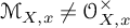 . It is the locus of points at which the log structure is non-trivial. For Y a log scheme with trivial log structure, any morphism
$Y \rightarrow X$
 to an fs log scheme lands in the open locus of points with trivial log structure
$X\setminus \partial X$
 . Thus there is a bijection between the set of logarithmic rational point of
$\mathrm {N}^{\mathrm {log}}_x(\underline {X},\underline {D})$
 and the set of rational points of
$\underline {\mathrm {N}}^{\mathrm {log}}_x(\underline {X},\underline {D})\setminus \partial \underline {\mathrm {N}}^{\mathrm {log}}_x(\underline {X},\underline {D}).$

To identify the open locus with trivial log strucure of the log normal space to D at x, note that it is the open subset on which any function
$m \in \mathcal {M}_{X}|_x$
 is inverted. Hence it is simply described as the spectrum of the localization of
$k[\mathcal {M}_{X}|_x]\otimes _{k[k^\times ]} k$
 at these elements (or at a set of generators of
$\mathcal {M}_{X}|_x$
 ). Therefore the open locus is

A rational point of this scheme is given in a unique way by a group morphism

which restricts to the identity on
$k^\times $
 . By the discussion above definition 2.1.4, this is what we wanted to prove.
Remark 2.1.8. If we let
$\mathrm {N}_x(\underline {X},\underline {D}_i):= \mathrm {Spec}(\mathrm {Sym}(\mathrm {T}_x\underline {X}/\mathrm {T}_x\underline {D}_i)^\vee )$
 there is a decomposition

so that the log structure is obtained via the product

Since the locus with non-trivial log structure of
$(\mathrm {N}_x(\underline {X},\underline {D}_i),0)$
 is reduced to the point
$\{0\}$
 , this point of view explains in another way that a logarithmic rational point of
$\mathrm {N}^{\mathrm {log}}_x(\underline {X},\underline {D})$
 is the same thing as a tangential basepoint at x: it is the datum of a vector
$v \in \mathrm {N}_x(\underline {X},\underline {D})$
 whose projection on each
$\mathrm {N}_x(\underline {X},\underline {D}_i)$
 does not vanish.
2.1.2 The functoriality of tangential basepoints
Since the construction
$\mathrm {N}^{\mathrm {log}}_x(\underline {X},\underline {D})$
 is functorial, it allows us to describe the functoriality for tangential basepoints.
Definition 2.1.9. A morphism
$f : (\underline {X},\underline {D}) \rightarrow (\underline {Y},\underline {E})$
 of divisorial log schemes over k satisfies
$f(\mathbf {x}) = \mathbf {y}$
 , with
$\mathbf {x}$
 and
$\mathbf {y}$
 tangential basepoints on
$ (\underline {X},\underline {D})$
 and
$(\underline {Y},\underline {E})$
 respectively if
$f(x) = y$
 , and if the induced morphism of log schemes
$\mathrm {N}_x^{\mathrm {log}}(\underline {X},\underline {D}) \rightarrow \mathrm {N}_y^{\mathrm {log}}(\underline {Y},\underline {E})$
 satisfies the condition that the following diagram commutes:

where the morphisms from
$\mathrm {Spec}(k)$
 are the log rational points associated with
$\mathbf {x}$
 and
$\mathbf {y}$
 by the lemma 2.1.7.
In a simple case, suppose
$(\underline {X},\underline {D}) = (\mathbb {A}^n,x_1\dots x_j= 0), (\underline {Y},\underline {E}) = (\mathbb {A}^m,y_1\dots y_k = 0)$
 and let
$f : (\underline {X},\underline {D}) \rightarrow (\underline {Y},\underline {E})$
 be a morphism of divisorial log schemes such that
$f(0) = 0$
 . There are monomials in the coordinates
$x_1,\dots , x_j$
 denoted by
$M_1, \dots , M_k \in K[x_1,\dots , x_j]$
 such that

If we let

be a tangential basepoint of
$(\underline {X},\underline {D})$
 at
$0$
 , then it is easy to see that the tangential basepoint defined by the composition

is

Remark 2.1.10. Note that in general, for
$f: (\underline {X},\underline {D}) \rightarrow (\underline {Y},\underline {E})$
 and
$\mathbf {x} := (x,t)$
 a tangential basepoint on
$(\underline {X},\underline {D})$
 , then
$f(\mathbf {x}) \neq (f(x), df_x(t))$
 . For instance if
$f: (\mathbb {A}^1,0) \rightarrow (\mathbb {A}^1,0)$
 is defined by
$f(x) = x^n$
 with
$ n \geq 2$
 , then
$df_0(t) = 0$
 while if
$t = \lambda \partial _x |_0$
 , then
$f(\mathbf {0}) = (0, \lambda ^n \partial _x |_0)$
 .
Remark 2.1.11. This functoriality seems to be aligned with, and was partly inspired by the point of view which consists in viewing tangential basepoints via morphisms
$\mathrm {Spec}(k((x))) \rightarrow X$
 , see for instance [Reference PetrovPet21, Lemma 10.1]. We will see in the next subsection another motivation for this functoriality.
2.1.3 The category of pointed diagrams
Let us now define the category of pointed diagrams which will be our framework when we define motivic tangential basepoints in subsection 3.3. Note that the diagram of log schemes over k

is functorial with respect to morphisms of divisorial log schemes over k.
Definition 2.1.12. We call the category of pointed diagrams the category whose objects are diagrams of log schemes over k of the form

where
$(\underline {X},\underline {D}) \in \mathbf {Div}_k$
 , and
$\mathbf {x}: \mathrm {Spec}(k) \rightarrow \mathrm {N}^{\mathrm {log}}_x(\underline {X},\underline {D})$
 is a tangential basepoint at a rational point x. To simplify, we denote such diagrams by
$(\underline {X},\underline {D},\mathbf {x})$
 .
A morphism of pointed diagrams
$(\underline {X},\underline {D},\mathbf {x}) \rightarrow (\underline {Y},\underline {E},\mathbf {y})$
 is a morphism of diagrams of log schemes over k given by a morphism of divisorial log schemes
$f: (\underline {X},\underline {D}) \rightarrow (\underline {Y},\underline {E})$
 sending x to y, the induced morphism of log schemes
$x^{\mathrm {log}} \rightarrow y^{\mathrm {log}}$
 , the induced morphism
$\mathrm {N}^{\mathrm {log}}_x(\underline {X},\underline {D}) \rightarrow \mathrm {N}^{\mathrm {log}}_y(\underline {Y},\underline {E})$
 and the identity on
$\mathrm {Spec}(k)$
 . In particular the diagram

must commute, which just means that
$f(\mathbf {x}) = \mathbf {y}$
 .
Hence, it is clear that the category of pointed diagrams is equivalent to the category of tangentially pointed smooth schemes over k with simple normal crossings divisor, that is the category whose objects are the datum of a divisorial log scheme
$(\underline {X},\underline {D})$
 over k and a tangential basepoint for
$(\underline {X},\underline {D})$
 , and whose morphisms are morphisms of divisorial log schemes over k which are compatible with the fixed tangential basepoints in the sense described above. The reason why we focus on the category of pointed diagrams lies in the fact that pointed diagrams are a higher dimensional and functorial analogue of Deligne’s gluing procedure to view tangential basepoints as points. Indeed if we apply the Kato–Nakayama space functor to the diagram (4) with
$X:= (\underline {X},\underline {D})$
 a smooth curve over k, we get

where, as in the introduction of this article,
$\mathrm {Bl}^{\mathbb {R}}$
 stands for the real-oriented blow-up. Deligne’s picture is simply the topological pushout of this diagram.
2.2 Virtual points
Now we connect our approach of tangential basepoints via logarithmic geometry to the point of view developed in [Reference Dupont, Panzer and PymDPP24], based on the notion of virtual morphisms of log schemes first defined in [Reference HowellHow17] and [Reference ShuklinShu22]. This class of maps between log schemes enlarge the class of classical morphisms of logarithmic schemes and introduces for instance, maps from a log scheme with trivial log structure which do not land in the locus of points with trivial log structure (see the proof of lemma 2.1.7). This, as we will see is the case for virtual points.
Definition 2.2.1 [Reference Dupont, Panzer and PymDPP24, Definition 2.6]
Let
$X,Y \in \mathbf {lSch}_k$
 . A virtual morphism
$X \rightarrow Y$
 is a pair
$(\underline {\phi },\phi ^\flat )$
 consisting of a morphism of schemes
$\underline {\phi }: \underline {X} \rightarrow \underline {Y}$
 , and a morphism
$\phi ^\flat : \underline {\phi }^{-1}\mathcal {M}^{\mathrm {gp}}_Y \rightarrow \mathcal {M}^{\mathrm {gp}}_X$
 of sheaves of groups, making the following diagram commute:

We denote by
$\mkern1mu^{\mathbf {v}}\mathbf {lSch}_k$
 the category of fs log schemes with virtual morphisms between them.
A morphism of log schemes induces in a unique way a virtual morphism of log schemes so that
$\mathbf {lSch}_k$
 is a subcategory of
$\mkern1mu^{\mathbf {v}}\mathbf {lSch}_k$
 . In order to distinguish morphisms in
$\mathbf {lSch}_k$
 from those in
$\mkern1mu^{\mathbf {v}}\mathbf {lSch}_k$
 we call the former ordinary morphisms of log schemes.
Definition 2.2.2. We let
$\mathbf {Div}_{k}^{\mathbf {v}*/}$
 be the category of virtually pointed divisorial log schemes over k. It is the category of divisorial log schemes
$(\underline {X},\underline {D})$
 with a virtual morphism
$\mathrm {Spec}(k) \rightarrow (\underline {X},\underline {D})$
 and in which the morphisms are ordinary morphisms of log schemes commuting with the fixed virtual points.
We can relate the category of pointed diagrams and the category of virtually pointed divisorial log schemes over k:
Theorem 2.2.3 [Reference Dupont, Panzer and PymDPP24, Theorem 3.5]
For
$X \in \mathbf {Div}_k$
 , there is a bijection between tangential basepoints of X and virtual points of X.
Hence, tangential basepoints can be described by both virtual morphisms on divisorial log schemes over k and pointed diagrams. Nevertheless, pointed diagrams offer the advantage of being constructed using ordinary morphisms only, which is what we will need to work in a log motivic category. We have the functorial version of the theorem 2.2.3:
Proposition 2.2.4. The category
$\mathbf {Div}^{\mathbf {v}*/}_k$
 is equivalent to the category of pointed diagrams.
Proof. The proof of [Reference Dupont, Panzer and PymDPP24, Theorem 3.5] is based on the fact that the datum of a pointed diagram
$(\underline {X},\underline {D},\mathbf {x})$
 , and of a virtual morphism
$\mathrm {Spec}(k) \rightarrow (\underline {X},\underline {D})$
 landing on x are both equivalent in a natural way to morphisms of groups
$\mathcal {M}_{X}|_x^{\mathrm {gp}} \rightarrow k^\times $
 that restrict to the identity on
$k^\times .$

Based on the previous proposition, we will simply denote by the thick letter
$\mathbf {x}$
 the equivalent datum of:
-
• a tangential basepoint at $x\in \underline {X}(k),$
-
• a pointed diagram $(\underline {X},\underline {D},\mathbf {x}),$
-
• a virtual morphism $\mathrm {Spec}(k) \rightarrow X.$


There is a last (partial) representation of tangential basepoints when
$k \subset \mathbb {C}$
 . If
$\mathbf {x}: * \rightarrow X$
 is a virtual point, then, since the Kato–Nakayama space construction is functorial with respect to virtual morphisms [Reference Dupont, Panzer and PymDPP24, Proposition 4.2], this datum determines a point on
$X^{\mathrm {KN}}$
 . More precisely since
$X^{\mathrm {KN}}$
 is the real-oriented blow-up of
$\underline {X}$
 along
$\underline {D}$
 , this determines a point of
$(S^1)^j$
 where j is the number of irreducible components of
$\underline {D}$
 at x. Each coordinate of
$(S^1)^j$
 determines a direction normal to one of the irreducible components of
$\underline {D}$
 .
Example 2.2.5. If
$X = \mathbb {A}_{\mathbb {N}}$
 with coordinate t, if the image of a virtual point
$\mathbf {x}$
 is the origin, then it is determined by a constant
$\lambda \in k^\times .$
 The associated tangential basepoint is
$(x,\lambda \frac {\partial }{\partial t}\big |_x)$
 , and its associated point on
$\mathbb {A}_{\mathbb {N}}^{\mathrm {KN}}$
 is given by the coordinate
$\frac {\lambda }{|\lambda |}$
 on the infinitesimal unit circle at
$0$

In the previous example, we note that two virtual morphisms determined by two constants
$\lambda , a\lambda $
 where a is a strictly positive constant have the same associated point on the Kato–Nakayama space. Hence a point on the Kato–Nakayama is not as such equivalent to the datum of a tangential basepoint. This is actually related to a classical fact in the theory of the fundamental group. The Betti side of the Hodge structure on the prounipotent completion of the fundamental group only sees the direction of the tangential basepoints, since a change of parametrization of any path based at a tangential basepoint can change the tangent vector by multiplication by an arbitrary strictly positive constant. In section 5.3, we will recall from [Reference Dupont, Panzer and PymDPP23, Section 8.4] how the structure of manifold with log corners of the Kato–Nakayama space allows to complete this approach so that the missing datum is encoded in the manifold with log corners version of virtual morphisms.
3 Log motives and motivic tangential basepoints
In this section, after a brief reminder of the constructions of different
$\infty $
 -categories of log motives as stated in [Reference Binda, Park and Arne ØstværBPØ22], and the properties of their
$\mathbb {A}^1$
 -invariant versions, introduced in [Reference ParkPar22], we explain how log-cdh-descent allows us to define motivic tangential basepoints. These are the augmentations of the cohomological motive of a divisorial log scheme associated with a tangential basepoint. This will lie at the heart of our definition of the motivic pointed path space in the next section. In the first two subsections we simply recall what is defined in [Reference ParkPar22, Reference ParkPar24a, Reference ParkPar24b]. In the last subsection 3.3, we define the motivic tangential basepoints and we spend some time to ensure that our construction is functorial as expected. In this section, k is a fixed field.
3.1 Log motivic categories
Definition 3.1.1 [Reference Cisinski and DégliseCD19, Definition 1.4.2]
Let
$\mathbf {C}$
 be a (1-)category with
$\mathcal {P}$
 a class of morphisms which contains all isomorphisms and which is stable by pullback. A
$\mathcal {P}$
 -premotivic
$\infty $
 -category over
$\mathbf {C}$
 is a functor

such that
-
• For all $f\in \mathcal {P}$
,
$f^*:= \mathcal {T}(f)$
has a left adjoint
$f_\sharp $
, -
• for every cartesian square
the natural transformation$$ \begin{align*}f^{\prime}_\sharp g^{\prime*} \rightarrow g^*f_\sharp\end{align*} $$is an equivalence,
-
• for every morphism $f \in \mathcal {P}$
, the
$\mathcal {P}$
-projection $$ \begin{align*}f_\sharp((-)\otimes f^*(-)) \rightarrow f_\sharp(-) \otimes (-)\end{align*} $$is an equivalence.


Definition 3.1.2. For
$\mathcal {T}$
 any
$\mathcal {P}$
 -premotivic
$\infty $
 -category over
$\mathbf {C}$
 , and for
$S\in \mathbf {C}$
 we let

be the homological motive functor where we denote by
$\mathcal {P}/S$
 the full subcategory of
$\mathbf {C}/S$
 with objects the morphisms
$X \rightarrow S \in \mathcal {P}$
 . We also denote by

the cohomological motive functor. They are defined for
$f: X\rightarrow S \in \mathcal {P}$
 by

and for
$f \in \mathbf {C}/S$
 , if we let
$f_*$
 denote a right adjoint of
$f^*$
 (which exists since
$f^*$
 is colimit preserving by hypothesis) by

where
$\mathbf {1}_S \in \mathcal {T}(S)$
 is the unit for the monoidal structure.
These two constructions are dual to each other in the sense that

Remark 3.1.3. When
$S = \mathrm {Spec}(k)$
 , for k a field, and the context is clear we will drop the S in the notations
$h_S, M_S$
 .
Let us give the definitions leading to the premotivic
$\infty $
 -categories with which we will work.
Definition 3.1.4.
-
• Let $\text {s\'{e}t}$
be the
strict étale topology
on
$\mathbf {lSm}_S$
, that is the Grothendieck topology generated by strict étale morphisms. -
• Let $\text {sNis}$
be the strict Nisnevich topology on
$\mathbf {lSm}_S$
, that is the Grothendieck topology generated by covers of the form
$(p: Y\rightarrow X, j: X' \rightarrow X)$
where p and j appear in a cartesian square where j is an open immersion and p is a strict étale morphism inducing an isomorphism$$ \begin{align*}p^{-1}(X\setminus X') \simeq X\setminus X'.\end{align*} $$
-
• Let $\mathrm {dNis}$
(resp.
$\text {d\'{e}t}$
) be the dividing Nisnevich topology (resp. the dividing étale topology
) on
$\mathbf {lSm}_S$
, that is the Grothendieck topology generated by
$\mathrm {sNis}$
(resp.
$\text {s\'{e}t}$
) and dividing covers, that is log étale, proper monomorphisms
$p: Y \rightarrow X$
. -
• Let $\mathrm {ver}_S$
be the family of open immersions
$U\rightarrow V$
such that
$U\setminus \partial _S U \rightarrow V\setminus \partial _S V$
is an isomorphism, where
$\partial _S$
defines the vertical boundary over S, i.e. the points with an open neighbourhood on which the structure morphism to S admits a Zariski local vertical chart [Reference OgusOgu18, Definition I.4.3.1].





The strict étale and Nisnevich topology are natural log versions of the classical étale and Nisnevich topology on
$\mathbf {Sm}_S$
 and the dividing topology encompasses log blow-ups. When S has trivial log structure, the
$\mathrm {ver}_S$
 topology is generated by open immersions
$U\setminus \partial U \rightarrow U$
 so that sheaves in this topology are canonically equivalent to presheaves on
$\mathbf {Sm}_S$
 .
Definition 3.1.5 [Reference RobaloRob12, Remark 4.12]
Let
$\mathcal {C}$
 be a presentable symmetric monoidal
$\infty $
 -category, and X an object of
$\mathcal {C}$
 . The stabilization
$\mathrm {Stab}_X(\mathcal {C})$
 of
$\mathcal {C}$
 by X is defined as

where
$\Omega _X:= \underline {\operatorname {Map}}(X,-)$
 is the internal mapping space, where
$\Sigma _X = - \otimes X$
 and where the limit is taken in
$\mathcal {C}\mathrm {at}_\infty $
 and the colimit in
$\mathcal {P}\mathrm {r}^{\mathrm {L}}$
 .
The recent work of Park culminated in [Reference ParkPar24b], where he managed to extend the classical six-functor formalism derived from the
$\mathbf {Sm}$
 -premotivic
$\infty $
 -category

where
$\mathbb {G}_m/1 := \mathrm {cofib}(M_S(*) \xrightarrow {1} M_S(\mathbb {G}_m))$
 and
$\mathrm {L}_{\mathbb {A}^1}$
 denotes the
$\mathbb {A}^1$
 localization, into a full six-functor formalism derived from a
$\mathbf {lSm}$
 -premotivic
$\infty $
 -category over
$\mathbf {lSch}$
 . This structure will be the main framework for our constructions.
Definition 3.1.6 [Reference ParkPar22, Definition 2.5.5]
The
$\mathbf {lSm}$
 -premotivic
$\infty $
 -category of motivic sheaves on
$\mathbf {lSch}$
 with coefficients in
$\Lambda $
 is defined by (the
$\otimes $
 highlights the symmetric monoidal structure)

and the
$\mathbf {lSm}$
 -premotivic stable homotopy
$\infty $
 -category of motivic sheaves by

where
$\mathbb {G}_m^{\mathrm {log}}/1:= \mathrm {cofib}(M_S(*) \xrightarrow {1} M_S(\mathbb {G}_m^{\mathrm {log}})) \in \mathrm {L}_{\mathbb {A}^1}\mathrm {L}_{\mathrm {ver}}\mathcal {S}\mathrm {h}_{\mathrm {dNis}}(\mathbf {lSm}_-,\mathcal {M}\mathrm {od}_\Lambda )$
 , with
$\mathbb {G}^{\mathrm {log}}_m:= (\mathbb {P}^1,\{0,\infty \})$
 .
From [Reference ParkPar22, Construction 2.5.4], when
$S \in \mathbf {Sch}$
 , there is a natural adjunction

defined by
$\lambda (X) = (X,\mathcal {O}^\times _X)$
 for
$X\in \mathbf {Sm}_S$
 and
$\omega (X) = X \setminus \partial X$
 for
$X\in \mathbf {lSm}_S$
 . It is easy to see that since the induced functor

satisfies
$\lambda ^*y_X \simeq y_{\omega (X)}$
 where y denotes the Yoneda functor, so that it induces a functor

Proposition 3.1.7 [Reference ParkPar22, Construction 2.5.4]
The functor
$\lambda ^*$
 is an equivalence

Remark 3.1.8. This is straightforward once we know that
$\omega $
 trivializes dividing and ver covers, and sends
$\mathbb {G}_m^{\mathrm {log}}$
 to
$\mathbb {G}_m$
 .
We keep separate notations
$\mathcal {DA}^{\mathrm {log}}$
 and
$\mathcal {DA}$
 even on log schemes with trivial log structures to distinguish the realization functors on each of these categories, see section 6. We will also refer to the étale version of the previous construction in the case of rational coefficients:
Definition 3.1.9. For
$S\in \mathbf {lSch}$
 , the
$\infty $
 -category of étale motivic sheaves on
$\mathbf {lSm}_S$
 with
$\mathbb {Q}$
 coefficients is defined by

When
$S\in \mathbf {Sch}$
 , the same proof as the proposition 3.1.7 gives the same result in this context, so that there is a commutative diagram in
$\mathrm {CAlg}(\mathcal {P}\mathrm {r}^{\mathrm {L}})$


with the functor induced by the étale sheafification on the horizontal arrows.
Remark 3.1.10. Since the category of étale log motives is not defined in Park’s work and for the sake of generality, we will work mainly in
$\mathcal {DA}^{\mathrm {log}}(S,\Lambda )$
 , and go to
$\mathcal {DA}^{\mathrm {log}}_{\text {\'{e}t}}(S,\mathbb {Q})$
 only to define the motivic fundamental groupoid in the mixed Tate case (see subsection 4.3). One should keep in mind that the definitions we make should work exactly the same in
$\mathcal {DA}^{\mathrm {log}}_{\text {\'{e}t}}(S,\mathbb {Q})$
 , so that the rest of the ideas developed in this article work when
$\mathcal {DA}^{\mathrm {log}}$
 is replaced with
$\mathcal {DA}^{\mathrm {log}}_{\text {\'{e}t}}$
 . Note that we took
$\mathbb {Q}$
 coefficients to avoid introducing hypersheaves, hence to simplify the exposition. With more general coefficients, the right definition would involve étale hypersheaves rather than étale sheaves, and these definitions do not coincide in general. They do however with
$\mathbb {Q}$
 coefficients, see [Reference Binda, Park and Arne ØstværBPØ25, Remark 2.6.3] (note that the same argument works with the étale topology instead of the strict étale topology).
3.2 log-cdh-descent for log motives
For
$S \in \mathbf {lSch}$
 , in [Reference ParkPar24a], Park shows that
$\mathcal {DA}^{\mathrm {log}}(S,\Lambda )$
 satisfies a log version of cdh-descent:
Definition 3.2.1. A commutative square of log-schemes over S

is a log-cdh distinguished square if it is a cartesian square, i is a strict closed immersion, p is proper, and the induced morphism
$p^{-1}(X\setminus i(Z)) \rightarrow X \setminus i(Z)$
 is an isomorphism.
Proposition 3.2.2 [Reference ParkPar24a, Corollary 3.6.8]
For any log-cdh distinguished square as in definition 7.1, the commutative square of functors

with
$q:= i \circ p'$
 , is cartesian.
From this proposition, if we denote by
$f: X \rightarrow S$
 ,
$g: X' \rightarrow S$
 ,
$h: Z' \rightarrow S$
 the structure morphisms, knowing that the pushforward and the pullback along a log smooth morphism are right adjoints, and hence preserve cartesian squares, the following square is cartesian:

Evaluating at
$\mathbf {1}_S$
 , we thus have that the square

is cartesian. This implies the following in the case where
$S = \mathrm {Spec}(k)$
 :
Corollary 3.2.3. The inclusion of the boundary of
$\mathbb {A}_{\mathbb {N}}$
 induces an equivalence in
$\mathcal {DA}^{\mathrm {log}}(k,\Lambda )$


Proof. We apply the previous discussion to the following log-cdh square:

with i the inclusion of the zero point, and p the morphism forgetting the log structure. Therefore we see that the square

is cartesian (and cocartesian by stability of
$\mathcal {DA}^{\mathrm {log}}(k,\Lambda )$
 ). Since the top arrow is an equivalence, the lemma is proved.
It is not clear in general that the functor h satisfies Künneth’s isomorphism. It obviously does on log smooth log schemes over k since h is the dual of M, but we will need it for the log point
$*_{\mathbb {N}^{n+m}} \simeq *_{\mathbb {N}^{n}} \times _k *_{\mathbb {N}^{m}}$
 which is non-log-smooth on k. This is the content of the following lemma.
Lemma 3.2.4. Let
$n,m$
 be two nonnegative integers. The natural morphism

is an isomorphism.
Proof. Let us consider the following cartesian square:

The classical proof of Künneth’s isomorphism in the context of a six functors formalism (see [Reference ScholzeSch22, Theorem 1.2]) relies on the projection formulae for the pushforwards

and

and on the base change isomorphism

Since all of the maps in the cartesian square are proper (i.e. their underlying morphism of schemes is proper), the three previous isomorphisms hold by [Reference ParkPar24a, Corollary 3.7.6, Theorem 3.7.8, Theorem 1.2.2].
Corollary 3.2.5. Let
$(\underline {X},\underline {D}) \in \mathbf {Div}_k$
 , and
$x\in \underline {X}(k)$
 , the natural closed immersion
$x^{\mathrm {log}} \rightarrow \mathrm {N}_x^{\mathrm {log}}(\underline {X},\underline {D})$
 induces a natural equivalence

Proof. By the description of the log normal space given after the definition 2.1.4, we know that
$\mathrm {N}_x^{\mathrm {log}}(\underline {X},\underline {D}) \simeq \mathbb {A}_{\mathbb {N}^j}$
 and
$x^{\mathrm {log}} \simeq *_{\mathbb {N}^j}$
 so that this corollary reduces to the corollary 3.2.3 thanks to the previous lemma.
3.3 Motivic tangential basepoints
We can now build a functor

allowing an extension of the classical construction of the augmentation
$h(X) \rightarrow \Lambda $
 associated to a point
$x\in \underline {X}(k)$
 to the case of tangential basepoints and thus enhancing the functor induced by the cohomological motive functor at the level of arrows

Definition 3.3.1. We let
-
• $\Delta [1]$
be the category -
• $\widetilde {\Delta [2]}$
be the category -
• $\Delta [2]$
be the category -
• $\overset {\leftarrow }{\Delta [3]}$
be the category


Remark 3.3.2. There is a sequence of functors

where the first morphism is the
$1$
 -face map and the second contracts the middle morphism.
The category
$\mathbf {Div}_{k}^{\mathbf {v}*/}$
 , viewed as the category of pointed diagrams (proposition 2.2.4), is a subcategory of
$\mathbf {Div}_k^{\overset {\leftarrow }{\Delta [3]}}$
 , so that there is a natural functor induced by the cohomological motive functor

Since the image of this composition lands in
$\mathcal {DA}^{\mathrm {log}}(k,\Lambda )^{\widetilde {\Delta [2]}}$
 , there is an induced morphism

by the following lemma:
Lemma 3.3.3. The functor

induced by the inclusion
$\overset {\leftarrow }{\Delta [3]} \rightarrow \widetilde {\Delta [2]}$
 is fully faithful.
Proof. The functor
$\overset {\leftarrow }{\Delta [3]} \rightarrow \widetilde {\Delta [2]}$
 is the
$1$
 -categorical localization of the category
$\overset {\leftarrow }{\Delta [3]}$
 by the middle morphism. Note that this is given by the pushout of the following diagram

where the horizontal morphism selects the middle morphism and
$\Delta [1]^\simeq $
 is the groupoid associated to
$\Delta [1]$
 .
The category
$\widetilde {\Delta [2]}$
 is still the pushout of this diagram in
$\mathcal {C}\mathrm {at}_\infty $
 after application of the nerve functor. This is not straightforward since the nerve functor does not preserve pushouts in general, see [Reference Hackney, Ozornova, Riehl and RovelliHORR24, Figure 1.1] for a counterexample, but it can be checked by computing the pushout explicitly.
More precisely, if we denote by
$\mathcal {C}$
 the pushout of the diagram above, there is a canonical arrow
$\mathcal {C} \rightarrow \widetilde {\Delta [2]}$
 . Note that the objects of
$\mathcal {C}$
 are given by the pushouts of objects of the categories involved in the diagram, as can be checked by applying the homotopy category functor
$ho(-)$
 to it (note that as a left adjoint to the nerve functor it preserves colimits). Now, since the functor
$\displaystyle \Delta [1] \rightarrow \overset {\leftarrow }{\Delta [3]}$
 is fully faithful, we can describe all the mapping spaces of
$\mathcal {C}$
 using [Reference Haine, Ramzi and SteinebrunnerHRS25, Theorem 0.1] which are all straightforwardly shown to be weakly equivalent to the corresponding mapping space in
$\widetilde {\Delta [2]}$
 (they are actually homeomorphic since they are reduced to a point, or empty). Hence the functor
$\mathcal {C}\rightarrow \widetilde {\Delta [2]}$
 is an equivalence of
$\infty $
 -categories.
This shows that, as
$\infty $
 -categories,
$\widetilde {\Delta [2]}$
 is the Dwyer–Kan localization of
$\overset {\leftarrow }{\Delta [3]}$
 along the middle morphism, see [Reference LandLan21, Proposition 2.4.8]. The lemma now comes from the universal property of localization [Reference LandLan21, Definition 2.4.2].
Hence, the cohomological motive functor defines a functor after composing with the sequence from remark 3.3.2:

Since
$\mathrm {CAlg}(\mathcal {DA}^{\mathrm {log}}(k,\Lambda ))^{/\Lambda }$
 is the faithful subcategory of
$\mathrm {Arr}(\mathrm {CAlg}(\mathcal {DA}^{\mathrm {log}}(k,\Lambda )))$
 consisting of arrows whose codomain is
$\Lambda $
 , and since this category is obtained as a fibre product of
$\mathrm {CAlg}(\mathcal {DA}^{\mathrm {log}}(k,\Lambda ))^{\Delta [1]}$
 and the point category on
$\mathrm {CAlg}(\mathcal {DA}^{\mathrm {log}}(k,\Lambda ))$
 , this defines a functor

Remark 3.3.4. Note that this construction is in fact defined only up to homotopy. More precisely, it depends on a choice of a quasi-inverse
$\Delta [2] \rightarrow \tilde {\Delta [2]}$
 to the contraction of the middle morphism. Two different choices lead to homotopy equivalent constructions.
Definition 3.3.5. We call motivic tangential augmentation (or motivic tangential basepoint) functor the functor

given by the composition of the sequence of arrows on the right. We denote by
$h(\mathbf {x}): h(X) \rightarrow \Lambda $
 the resulting arrow.
Remark 3.3.6. In a more direct fashion, from a diagram

by a choice of homotopy inverse of the central equivalence, we get a diagram

that we compose to get an augmentation
$h(X) \rightarrow \Lambda $
 .
This construction actually works in the same way in any ‘category of log motives’ in which the cohomological motives of the standard log point and of
$\mathbb {A}_{\mathbb {N}}$
 are equivalent, and in which Künneth’s isomorphism holds for the cohomological motives of products of the log point.
Remark 3.3.7. Note that if
$\mathbf {x}$
 is just given by a rational point
$x \in \underline {X}(k)\setminus \underline {D}(k)$
 , then the motivic augmentation defined by
$\mathbf {x}$
 is the classical augmentation
$h(x)$
 . Indeed the pointed diagram associated with
$\mathbf {x}$
 is

so that the morphism

is the expected one.
4 The motivic fundamental group
In this section, we describe in detail properties of the bar construction in an
$\infty $
 -categorical context, and we use it to construct the motivic pointed path space based at tangential basepoints. In particular, we highlight the resulting homotopy Hopf algebroid structure of the datum of the motivic pointed path spaces based at tangential basepoints. We compare this construction with Wojtkowiak’s approach [Reference WojtkowiakWoj93] recalled in the introduction, which will be useful to compute the realizations of the motivic pointed path space in the next section. We end this section with the mixed Tate case which leads to the definition of the motivic fundamental torsor at tangential basepoints. The key points of this section are the theorem 4.1.9, definition 4.2.1 and proposition 4.2.7. In this section, k is still a fixed field.
4.1 The bar construction
Let us first summarize facts about the bar construction. In this section, nothing is new except the description of the homotopy Hopf algebroid structure in an
$\infty $
 -categorical context. The main reference here is [Reference LurieLur17, Sections 4.4.2, 5.2.2].
Let
$\mathcal {C}$
 be a cocomplete symmetric monoidal
$\infty $
 -category such that the tensor product
$\otimes : \mathcal {C} \times \mathcal {C} \rightarrow \mathcal {C}$
 commutes with colimits in each variable.
Proposition 4.1.1 [Reference LurieLur17, Construction 4.4.2.7, Example 4.4.2.11]
For
$A \in \mathrm {CAlg}(\mathcal {C})$
 ,
$M,N\in \mathrm {Mod}_A(\mathcal {C})$
 , there is a canonical simplicial diagram
$\mathrm {Bar}_A(M,N)_\bullet $
 in
$\mathrm {Mod}_A(\mathcal {C})$
 informally given by:

such that its colimit is the relative tensor product of M and N over A:

It is the bar construction of A on M and N.
Degreewise
$\mathrm {Bar}_A(M,N)_n \simeq M \otimes A^n \otimes N$
 with face maps induced by the product

and the actions on M and N

The degeneracies are given by the unit map

For
$A \in \mathrm {CAlg}(\mathcal {C})$
 , the relative tensor product over A endows the category
$\mathrm {Mod}_A(\mathcal {C})$
 with a symmetric monoidal
$\infty $
 -category structure [Reference LurieLur09, Theorem 4.5.2.1].
We will apply the relative tensor product in a more restrictive case, that is when A is a biaugmented commutative algebra object in
$\mathcal {C}$
 with augmentations (i.e. algebra morphisms)
 . We denote by
$\mathbf {1}_x, \mathbf {1}_y$
 the unit element of
$\mathcal {C}^\otimes $
 viewed as commutative A-algebras through the maps x and y.
Definition 4.1.2. We call bar construction of A based at x and y the object

Remark 4.1.3. The choice for the order of the entries is a convention explained in remark 4.2.2.
We recall that this object comes with a natural structure of commutative A-algebra object in
$\mathcal {C}$
 . Indeed, by applying [Reference LurieLur17, Proposition 3.2.4.7, Corollary 3.2.4.8] to
$\mathrm {Mod}_A(\mathcal {C})$
 , we see that
$\mathrm {CAlg}_A(\mathcal {C}) = \mathrm {CAlg}(\mathrm {Mod}_A(\mathcal {C}))$
 has coproducts and that these coproducts coincide with iterated relative tensor products.
In particular,

This way, it is easy to see that the bar construction defines a functor

Note that the A-algebra structure is defined by the map
$\mkern1mu_x\nabla _y$
 described by

and by the natural map

Let us recall the definition of a homotopy Hopf algebra in an
$\infty $
 -category in the sense of [Reference ErgusErg22, Definition 4.0.1, Corollary 4.1.4], which is a bialgebra with a homotopy antipode. We remind the reader that the category of bialgebra objects in
$\mathcal {C}$
 is defined to be
$\mathrm {Alg}(\mathrm {CAlg}(\mathcal {C})^{\mathrm {op}}).$

Definition 4.1.4. A homotopy Hopf algebra object
$H \in \mathcal {C}$
 is a bialgebra object endowed with a map

such that H is a Hopf algebra in the homotopy category of
$\mathcal {C}$
 with antipode s.
We now prove a general structure result for the bar construction:
Theorem 4.1.5. The datum of the objects and morphisms
$\{\mkern1mu_x\mathrm {Bar}_y(A)\}_{x,y}$
 for all augmentations
$x,y$
 of A is enhanced into a homotopy Hopf algebroid, i.e.
-
• For all augmentations x, $\mkern1mu_x\mathrm {Bar}_x(A)$
has the structure of a homotopy Hopf algebra in
$\mathcal {C}.$
-
• For three augmentations $x,y,z$
, there is a deconcatenation map $$ \begin{align*}\mkern1mu^{}_x\Delta_z^y \;: \;_x\mathrm{Bar}_z(A) \rightarrow \;_y\mathrm{Bar}_z(A) \otimes \,_x\mathrm{Bar}_y(A)\end{align*} $$which is the coproduct on $\;_x\mathrm {Bar}_x(A)$
when
$x = y = z$
.
-
• For all augmentations $x,y$
, there is an involution $$ \begin{align*}\!_xs_y: \;_x\mathrm{Bar}_y(A) \rightarrow \;_y\mathrm{Bar}_x(A)\end{align*} $$which is the homotopy antipode of $\;_x\mathrm {Bar}_x(A)$
when
$x = y$
.
-
• If we let $\epsilon _x: \mkern1mu_x\mathrm {Bar}_x(A) \rightarrow \mathbf {1}$
denote the counit of
$\mkern1mu_x\mathrm {Bar}_x(A)$
for all augmentations x, then the morphisms $$ \begin{align*}\{\mkern1mu_x\nabla_y, \mkern1mu_x\eta_y, \mkern1mu^{}_x\Delta_z^y, \mkern1mu_xs_y, \epsilon_x\}_{x,y,z}\end{align*} $$satisfy the homotopy counit, coinverse and coassociativity axioms which respectively state that in the homotopy category $\mathrm {ho}(\mathcal {C})$
-
– $(\epsilon _y \otimes \mathrm {Id})\circ \mkern1mu^{}_x\Delta _y^y = \mathrm {Id}$
and
$(\mathrm {Id} \otimes \epsilon _x)\circ \mkern1mu^{}_x\Delta _y^x = \mathrm {Id},$
-
– $\mkern1mu_x\nabla _y\circ (\mkern1mu_ys_x \otimes \mathrm {Id})\circ \mkern1mu^{}_x\Delta _y^x = \mkern1mu_y\eta _x\circ \epsilon _x$
and
$\mkern1mu_y\nabla _x\circ (\mathrm {Id} \otimes \mkern1mu_xs_y )\circ \mkern1mu^{}_x\Delta _y^x = \mkern1mu_x\eta _y \circ \epsilon _x$
, -
– for $x,y,z,t$
four augmentations of A,
$(\mkern1mu^{}_y\Delta _t^z \otimes \mathrm {Id})\circ \mkern1mu^{}_x\Delta _t^y = (\mathrm {Id} \otimes \mkern1mu^{}_x\Delta _z^y)\circ \mkern1mu^{}_x\Delta _t^z$
.
-






This theorem shows that the data of the pointed bar constructions of A, taken over all augmentations of A, carries a structure dual to that of a groupoid in the homotopy category of
$\mathcal {C}$
 . Here, by a groupoid structure we mean the one carried for instance by the system of pointed path spaces of a topological space X: namely, the collection of all pointed path spaces of X, together with the associative composition of paths, the existence of inverse paths, and the unit path at each point of X. It is in this sense that we will interpret and work with the notion of a homotopy Hopf algebroid in the following sections. In particular, in subsection 4.3 we will define the motivic analogue of the fundamental groupoid in the presence of a motivic t-structure.
Note that we have defined the structure of a homotopy Hopf algebroid only in a weak homotopical sense. In an
$\infty $
 -categorical framework, one would usually formalize such a structure by verifying all possible higher coherences, so our notion is not as rigorous as it could be in that setting. However, lifting this definition to an
$\infty $
 -categorical level lies beyond the scope of this article, as we only require the structure to be well defined in the homotopy category of
$\mathcal {C}$
 .
The rest of this subsection is dedicated to the proof of theorem 4.1.5. This proof consists in the lemmas 4.1.6, 4.1.7, 4.1.8, 4.1.9 and 4.1.10.
Let us first describe the
$\infty $
 -categorical structure of bialgebra that completes the structure of commutative algebra object of the pointed bar construction:
Lemma 4.1.6. Let
$A \in \mathrm {CAlg}(\mathcal {C})$
 . For each augmentation
$x: A \rightarrow \mathbf {1}$
 ,
$\mkern1mu_x\mathrm {Bar}_x(A)$
 has a natural associative bialgebra structure.
The complete and careful proof of this fact is [Reference LurieLur17, Theorem 5.2.2.17], where the bar construction is enhanced into a functor

which shows that the bar construction over a single augmentation has a natural coalgebra structure. The commutative algebra and coalgebra structures are compatible since the commutative algebra structure can be directly derived from the previous functor: Since

[Reference LurieLur17, Corollary 2.4.3.10], we can apply the bar construction directly in
$\mathrm {CAlg}(\mathcal {C})$
 which gives a functor

Since the forgetful functor
$\mathrm {CAlg}(\mathcal {C}) \rightarrow \mathcal {C}$
 commutes with colimits of simplicial diagrams [Reference LurieLur17, Corollary 3.2.3.2], we have that
$\mathrm {Bar} = \mathrm {Bar}'$
 .
The coproduct inducing the bialgebra structure of the bar construction can be derived from the more general deconcatenation map:
Lemma 4.1.7. Suppose A has three augmentations
$x,y,z$
 . Then there is a natural deconcatenation map in
$\mathrm {CAlg}(\mathrm {Mod}_A(\mathcal {C}))$


Proof. The map is built as follows:

Note that the line 4 uses both the associativity and commutativity of the relative tensor product and a change of base algebra [Reference LurieLur17, Section 4.5.3].
Over a single augmentation x, the deconcatenation map is the coproduct map on the bar construction of A over x. Note that there is as well a canonical augmentation given by the natural morphism

We can readily prove the counit axiom:
Lemma 4.1.8. For
$x,y$
 augmentations of A, the following equality

and

hold in the homotopy category of
$\mathcal {C}$
 .
Proof. Let us treat the first case, as the second one is similar. The composition is

This morphism is given by the canonical morphism

and by the morphism on the left component

which is the identity by the algebra structure of
$\mathbf {1}_y \otimes _A \mathbf {1}_y$
 .
Let us now consider the involution

exchanging the two augmentations. Then, we can check the coinverse axiom. This proves in particular that
$\mkern1mu_x\mathrm {Bar}_x(A)$
 is a homotopy Hopf algebra for all augmentations x of A.
Lemma 4.1.9. The commutative algebras
$\mkern1mu_x\mathrm {Bar}_x(A)$
 ,
$\mkern1mu_x\mathrm {Bar}_y(A)$
 and
$\mkern1mu_y\mathrm {Bar}_x(A)$
 equipped with the deconcatenation
$\mkern1mu_x^{}\Delta _x^y$
 , product
$\mkern1mu_x\nabla _y$
 , unit
$\mkern1mu_x\eta _y: \mathbf {1} \rightarrow \mkern1mu_x\mathrm {Bar}_y(A)$
 , counit
$\epsilon _x: \mkern1mu_x\mathrm {Bar}_x(A) \rightarrow \mathbf {1}$
 and involution
$\mkern1mu_xs_y$
 fit in the homotopy commutative diagrams:

and

Proof. We only prove the lemma in the upper diagram since the other case works in the same way. The upper composition can be described by the sequence

where the last arrow is identified with the componentwise product. Note that this last arrow can be described by the change of base ring equivalence [Reference LurieLur17, 4.5.3]:

where the last arrow is induced by the product on
$\mathbf {1}_x$
 . Then the full composition is homotopic to the composition

where the last arrow is again induced by the product on
$\mathbf {1}_x$
 . This is itself identified with the map

and this composition is homotopic to
$\mkern1mu_y\eta _x\circ \epsilon _x$
 .
Finally it remains to check the coassociativity axiom:
Lemma 4.1.10. Let
$x,y,z,t$
 four augmentations of A. Then the equality

holds in the homotopy category of
$\mathcal {C}$
 .
Proof. The lemma is proved by checking that the two compositions are described (up to associativity of the tensor product) by the composition

and then two successive changes of base algebras.
Remark 4.1.11. In their recent work, I. Dan-Cohen and A. Horev proved that [Reference Dan-Cohen and HorevDCH22, Corollary 8.4.3] the deconcatenation maps from lemma 4.1.7 endow
$\mkern1mu_{x}\mathrm {Bar}_{y}(A)$
 with a left (resp. right) coalgebra structure under the coaction of
$\mkern1mu_{x}\mathrm {Bar}_{x}(A)$
 (resp.
$\mkern1mu_{y}\mathrm {Bar}_{y}(A)$
 ). This lifts part of the structure described above
$\infty $
 -categorically.
Remark 4.1.12. Since it is defined as the colimit of a simplicial object in
$\mathcal {C}$
 , the bar construction is a filtered object in
$\mathcal {C}$
 [Reference LurieLur17, Remark 1.2.4.2]. The filtration is given by the geometric realization of skeletons that we denote for
$n \in \mathbb {N}$
 by

In a
$1$
 -categorical context,
$\mkern1mu_x\mathrm {Bar}_x(A)$
 has a structure of filtered Hopf algebra since the operations we introduced are compatible with the filtration, see [Reference WojtkowiakWoj93], [Reference Ignacio Burgos Gil and FresánBGF25, Section 3.5] for a full description. Furthermore,
$\mkern1mu_x\mathrm {Bar}_y(A)$
 has the structure of a filtered comodule under the coactions of
$\mkern1mu_x\mathrm {Bar}_x(A)$
 and
$\mkern1mu_y\mathrm {Bar}_y(A)$
 . We do not know if such a result can be extended to an
$\infty $
 -categorical context, but we will not need it in the rest of this paper, since we will only describe the filtered structure at the level of realizations.
Example 4.1.13. Let us detail the construction in the classical case of a commutative differential graded algebra A, viewed as an object of the
$\infty $
 -category of chain complexes over a field K, endowed with two augmentations
$x,y: A \rightarrow K$
 , since this will come in handy in the computation of the realizations of the motivic fundamental groupoid. By [Reference ArakawaAra23, Corollary 3.13], the geometric realization of a simplicial object
$X_\bullet $
 in
$\mathcal {M}\mathrm {od}_K$
 is given by the total complex associated with the bicomplex
$\mathrm {M}(X_\bullet )$
 where
$\mathrm {M}$
 is the Moore complex functor. Hence,

If we use cohomological conventions, then

Hence, a degree n element of the bar complex is denoted by

In this construction, the filtration on the bar complex is interpreted as the classical length filtration, that is
$\;_x\mathrm {Bar}_y(A)_{\leq k}$
 is the subcomplex spanned by elements of the form given above, with
$q \leq k$
 .
4.2 The motivic pointed path space based at tangential basepoints
We now have all the tools in hand to build the motivic pointed path space based at tangential basepoints. Let
$X\in \mathbf {Div}_k$
 ,
$\mathbf {x}, \mathbf {y}$
 two tangential basepoints of X and
$h(\mathbf {x}), h(\mathbf {y}): h(X) \rightarrow \Lambda $
 the corresponding motivic tangential augmentations. Then
$h(X)$
 has the structure of a biaugmented commutative algebra object in
$\mathcal {DA}^{\mathrm {log}}(k,\Lambda )$
 . We can then apply the bar construction to this datum.
Definition 4.2.1. We call the motivic pointed path space of X based at
$\mathbf {x}$
 and
$\mathbf {y}$
 the commutative algebra object

This determines a functor

Remark 4.2.2. We chose to put
$h(\mathbf {1}_{\mathbf {y}})$
 before
$h(\mathbf {1}_{\mathbf {x}})$
 in the tensor product to define the motivic path space from
$\mathbf {x}$
 to
$\mathbf {y}$
 in order to follow the convention chosen in [Reference Deligne and GoncharovDG05, Reference Ignacio Burgos Gil and FresánBGF25].
By the results of the previous subsection, the motivic based path spaces are a highly structured algebra in
$\mathcal {DA}^{\mathrm {log}}(k,\Lambda )$
 . Precisely, it is a straightforward consequence of theorem 4.1.9 that the following proposition holds:
Proposition 4.2.3. The family
$\{\mkern1mu^{}_{\mathbf {x}}\mathrm {P}^m_{\mathbf {y}}X\}_{\mathbf {x},\mathbf {y}}$
 for all tangential basepoints
$\mathbf {x},\mathbf {y}$
 has the structure of a homotopy Hopf algebroid in
$\mathcal {DA}^{\mathrm {log}}(k,\Lambda )$
 .
Remark 4.2.4. We draw inspiration from [Reference Dan-Cohen and SchlankDCS22], [Reference SpitzweckSpi10], and [Reference IwanariIwa20], where respectively I. Dan-Cohen and T. Schlank, M. Spitzweck, and I. Iwanari defined the motivic fundamental group in an
$\infty $
 -categorical/model theoretic context.
4.2.1 The cosimplicial pointed path space
When
$\mathbf {x}, \mathbf {y}$
 are ordinary basepoints, as mentioned in the introduction of this article, the definition of the motivic pointed path space in the case of ordinary basepoints as explained by Deligne and Goncharov in [Reference Deligne and GoncharovDG05] or by Levine and H. Esnault in [Reference Esnault and LevineEL11] relies on a translation to the language of algebraic geometry, due to Wojtkowiak in [Reference WojtkowiakWoj93], of the topological definition of the pointed path space. We generalize this definition in our context, since we will need it to compute the realization of the motivic pointed path space in the next section:
For
$X \in \mathbf {lSch}_k$
 let us consider the cosimplicial log scheme given by

For
$n \in \mathbb {N}$
 ,

the i-th coface map for
$0 \leq i \leq n+1$
 is given by

and the i-th codegeneracy map for
$0 \leq i \leq n-1$
 by the projection

Remark 4.2.5.
$X^{[0,1]}$
 comes equipped with a map

induced by the inclusion
$\partial \Delta [1] \subset \Delta [1]$
 , where the right term is the constant cosimplicial log scheme. This map is degreewise the projection on the first and last factor.
Definition 4.2.6. For
$\mathbf {x},\mathbf {y}$
 two tangential basepoints on
$X\in \mathbf {Div}_k$
 , we call cosimplicial path space of X based at
$\mathbf {x},\mathbf {y}$
 the cosimplicial object of
$\mkern1mu^{\mathbf {v}}\mathbf {lSch}_k$
 defined by the pullback

Let us explain how this fibre product is defined in the category of cosimplicial diagrams of log schemes with virtual morphisms between them. Its n-cosimplices are
$X^n$
 , the degeneracies are all the projections
$X^{n} \rightarrow X^{n-1}$
 , and the cofaces are the same as the ones in the upper description, except for the
$0$
 -th and the
$(n+1)$
 -th, defined by the product of the virtual point
$\mathbf {y}$
 with the identity of
$X^{n+1}$
 and by the product of the identity of
$X^{n+1}$
 with the virtual point
$\mathbf {x}$
 .
Since we cannot view this object in a log motivic formalism in a canonical way (there is no category of virtual log motives) we cannot compare the bar construction of
$h(X)$
 based at
$\mathbf {x},\mathbf {y}$
 with a simplicial motive associated with the cosimplicial path space based at
$\mathbf {x},\mathbf {y}$
 , as in the case with ordinary basepoints. Nevertheless we can check that our definition coincides with the latter in the case with ordinary basepoints.
Proposition 4.2.7. When
$\mathbf {x},\mathbf {y}$
 are rational points of
$\underline {X}\setminus \underline {D}$
 , there is a natural equivalence in
$\mathrm {CAlg} (\mathcal {DA}^{\mathrm {log}}(k,\Lambda ))$
 :

Proof. Once we check that the motivic augmentations associated with
$\mathbf {x},\mathbf {y}$
 are the usual augmentation associated with the corresponding rational points
$x,y$
 which is done in remark 3.3.7, this is a classical fact, proved in [Reference IwanariIwa20, Theorem A.7] for instance, or see the same proof applied in the Betti case in the discussion following theorem 5.2.11.
4.3 The motivic fundamental groupoid at tangential basepoints
We can now define the motivic fundamental groupoid based at tangential basepoints. Although we work in the context of mixed Tate motives, what follows works in a similar fashion in the general case of the existence of a motivic t-structure.
Recall that the triangulated category of mixed Tate motives over a field k is classically defined to be the smallest triangulated full subcategory of the triangulated category of mixed motives
à la Voevodsky
$\mathbf {DM}(k,\mathbb {Q})$
 [Reference VoevodskyVoe00] generated by the Tate objects
$\mathbb {Q}(n)$
 for
$n\in \mathbb {Z}$
 . In the language of
$\infty $
 -categories, the right definition is (see [Reference IwanariIwa20, Section 6.2] for details):
Definition 4.3.1. Let
$\mathcal {DM}(k,\mathbb {Q})$
 be the stable
$\infty $
 -category of mixed motives over k with
$\mathbb {Q}$
 coefficients (see for instance [Reference IwanariIwa20, Reference ParkPar22] for a definition). Then we let
$\mathcal {DMT}_{\mathrm {gm}}(k,\mathbb {Q})$
 be the smallest stable subcategory of
$\mathcal {DM}(k,\mathbb {Q})$
 generated by the Tate objects
$\mathbb {Q}(n)$
 . The stable
$\infty $
 -category of mixed Tate motives over k is the full subcategory of
$\mathcal {DM}(k,\mathbb {Q})$
 defined by

Suppose now that k satisfies the Beilinson–Soulé vanishing conjecture,
$\mathcal {DMT}(k,\mathbb {Q})$
 and
$\mathcal {DMT}_{\mathrm {gm}}(k,\mathbb {Q})$
 come with a t-structure [Reference LevineLev93], [Reference IwanariIwa14, Section 7] (defined on the homotopy categories see [Reference LurieLur17, Definition 1.2.1.4]). The heart of
$\mathcal {DMT}_{\mathrm {gm}}(k,\mathbb {Q})$
 is the neutral tannakian (1-)category of mixed Tate motives over k, denoted by
$\mathbf {MT}(k,\mathbb {Q})$
 . There is a
$0$
 -cohomology functor

The heart of the t-structure on
$\mathcal {DMT}(k,\mathbb {Q})$
 is
$\mathrm {Ind}\mathbf {MT}(k,\mathbb {Q})$
 and the corresponding
$0$
 -cohomology functor
$\mathcal {DMT}(k,\mathbb {Q})$
 is the indization of
$\mathrm {H}^0_{\mathrm {mot}}$
 .
Recall as well from [Reference Cisinski and DégliseCD19, Theorem 16.2.18, Theorem 16.1.4] that there is an equivalence of symmetric monoidal
$\infty $
 -categories

so that
$\mathcal {DMT}(k,\mathbb {Q})$
 can be viewed as a full subcategory of
$\mathcal {DA}_{\text {\'{e}t}}(k,\mathbb {Q})$
 .
Definition 4.3.2. We say that a log smooth log scheme X over k is of mixed Tate type if
$M^{\text {\'{e}t}}_k(X) \in \mathcal {DMT}(k,\mathbb {Q})$
 .
If
$X \in \mathbf {Div}_k$
 then the structure of homotopy Hopf algebroid of the family of motivic path spaces at tangential basepoint is preserved after étale localization, i.e. after applying the functor induced by étale sheafification. Furthermore, for
$\mathbf {x},\mathbf {y}$
 tangential basepoints on X, the motivic path space based at
$\mathbf {x},\mathbf {y}$
 is an element of
$\mathcal {DMT}(k,\mathbb {Q})$
 by definition. We now show that taking its
$0$
 -th cohomology group carries the whole structure to
$\mathrm {Ind}\mathbf {MT}(k,\mathbb {Q})$
 :
Theorem 4.3.3. The family of objects
$\{\mathrm {H}^0_{\mathrm {mot}}((\mkern1mu^{}_{\mathbf {x}}\mathrm {P}_{\mathbf {y}}^mX)^{\mathrm {\acute {e}t}})\}_{\mathbf {x},\mathbf {y}}$
 of
$\mathrm {Ind}\mathbf {MT}(k,\mathbb {Q})$
 has the structure of a Hopf algebroid deduced from the structure of theorem 4.1.5, i.e. the corresponding family in the opposite category
$\mathrm {Ind}\mathbf {MT}(k,\mathbb {Q})^{\mathrm {op}}$
 has a structure of a groupoid.
Proof. The only potential obstruction to this lies in the fact that the functor
$\mathrm {H}^0_{\mathrm {mot}}$
 is not symmetric monoidal. Let us show that for
$\mathbf {x,x',y,y'}$
 tangential basepoints on X it satisfies

This naturally implies the theorem. We know from [Reference BiglariBig07, Example 3.3.2] that the t-structure on
$\mathcal {DMT}_{\mathrm {gm}}(k,\mathbb {Q})$
 is compatible with the tensor structure, which implies that the family of cohomology functors
$\mathrm {H}^i_{\mathrm {mot}}$
 satisfies the Künneth formula.
It is now clear that it suffices to show that for
$\mathbf {x},\mathbf {y}$
 tangential baspoints on X, the cohomology in negative degrees of
$\mkern1mu^{}_{\mathbf {x}}\mathrm {P}_{\mathbf {y}}^mX$
 is zero. It suffices to check this for the filtered pieces
$\mkern1mu^{}_{\mathbf {x}}\mathrm {P}_{\mathbf {y}}^mX_{\leq n}$
 . We only need to check that the Betti realization of this motive is concentrated in nonpositive degree because the Betti realization of mixed Tate motives is conservative, see [Reference Deligne and GoncharovDG05, Proposition 2.14] (the fully faithfulness of the Hodge realization implies its conservativity, and hence the conservativity of the Betti realization). This is trivial from the description at the end of section 5.2.
From this, we are able to give the following definition of the motivic fundamental groupoid at tangential basepoints:
Definition 4.3.4. Let
$X \in \mathbf {Div}_k$
 , with tangential basepoints
$\mathbf {x},\mathbf {y}$
 , and suppose X is of mixed Tate type. Then the motivic fundamental torsor at
$\mathbf {x},\mathbf {y}$
 is defined by

Where
$\mathrm {Pro}\mathbf {MT}(k,\mathbb {Q})-\mathbf {Sch}$
 is the opposite of the category of commutative algebra objects in
$\mathrm {Ind}\mathbf {MT}(k,\mathbb {Q}).$

The following proposition is trivial from proposition 4.2.3
Proposition 4.3.5. The family of the motivic fundamental torsors
$\pi _1^m(X,\mathbf {x},\mathbf {y})$
 for all tangential basepoints
$\mathbf {x},\mathbf {y}$
 of X, equipped with the dual morphisms of the morphisms constructed in theorem 4.1.9, has the structure of a groupoid.
Precisely, for
$\mathbf {x},\mathbf {y},\mathbf {z}$
 three tangential basepoints of X, there is an operation of composition of paths

which is associative in the obvious sense, an isomorphism of inversion of paths

which yields an inverse for the composition of paths, and each

has the structure of a pro-
$\mathbf {MT}(k,\mathbb {Q})$
 group scheme. All these data satisfy the axioms dual to the axioms given in theorem 4.1.9.
We call the family
$\{\pi _1^m(X,\mathbf {x},\mathbf {y})\}_{\mathbf {x},\mathbf {y}}$
 equipped with the operations described above the motivic fundamental groupoid at tangential basepoints.
Remark 4.3.6. In particular, for all
$\mathbf {x,y}$
 tangential basepoints of X,
$\pi _1^m(X,\mathbf {x},\mathbf {y})$
 is endowed with a left (resp. right) action of
$\pi _1^m(X,\mathbf {x})$
 (resp.
$\pi _1^m(X,\mathbf {y})$
 ).
5 Realizations
In this last section, we show that the degree zero cohomology of the Betti and de Rham realizations of the motivic pointed path space recover the expected Betti–de Rham theory of the prounipotent completion of the fundamental torsor at tangential basepoints. To do so, in the first subsection we explain how to build realization functors for
$\mathbb {A}^1$
 -invariant log motives. An approach to do this in an
$\infty $
 -categorical context is to employ the language of mixed Weil cohomology theories. We follow and adapt Drew’s work in [Reference DrewDre18]. We compute the Betti (resp. the de Rham) realization functor, and we compute the realizations of the motivic pointed path space in the second subsection (resp. the third). In both cases we find explicit complexes representing this realization. We navigate between the different approaches of tangential basepoints explained in subsection 2.2, and between
$\infty $
 and
$1$
 -categories according to our needs. In the last subsection, we compute the periods of the motivic fundamental groupoid via the notion of regularized iterated integrals, adapted from regularized integration as defined in [Reference Dupont, Panzer and PymDPP23].
5.1 Realization functors
In this subsection, k is a field of characteristic
$0$
 . We can naturally generalize the definition of mixed Weil theories given in [Reference DrewDre18] to a log geometric context:
Definition 5.1.1. A
$\Lambda $
 -linear log mixed Weil theory over k is a symmetric monoidal functor
$\boldsymbol {\Gamma }^\otimes : \mathbf {lSm}_k^{op,\times } \rightarrow \mathcal {M}\mathrm {od}_\Lambda ^\otimes $
 such that if we let
$\boldsymbol {\Gamma }$
 be the underlying functor of
$\infty $
 -categories, the following conditions are satisfied:
-
• $\boldsymbol {\Gamma }$
has its values in
$\operatorname {Perf}(\Lambda )$
, the sub-
$\infty $
-category of bounded complexes of finite projective modules. -
• $\boldsymbol {\Gamma }$
is a
$\mathcal {M}\mathrm {od}_\Lambda $
-valued
$\mathrm {dNis}$
-sheaf. -
• $\boldsymbol {\Gamma }^{\mathrm {op}}: \mathbf {lSm}_k \rightarrow \mathcal {M}\mathrm {od}_\Lambda ^{\mathrm {op}}$
is
$\mathbb {A}^1$
-invariant and
$\mathrm {ver}$
-invariant. -
• $\boldsymbol {\Gamma }$
sends
$\mathrm {cofib}(1\rightarrow \mathbb {G}^{\mathrm {log}}_m)$
to a
$\otimes $
-invertible object.


Furthermore, we say that a log mixed Weil theory is an étale log mixed Weil theory if it is as well a strict étale sheaf.
Log mixed Weil theories, modelling log cohomology theories, are the starting point to build realization functors. We prove a logarithmic version of the theorem 3.7 in [Reference DrewDre18]. Note that it is a log and
$\Lambda $
 -linear version of [Reference RobaloRob15, Theorem 2.9]:
Proposition 5.1.2. The homological motive functor induces a homotopy equivalence of Kan complexes

The subscript
$\mathrm {P}^{\mathrm {log}}$
 means the subcomplex generated by the functors
$\boldsymbol {\Gamma }$
 such that
$\boldsymbol {\Gamma }^{\mathrm {op}}$
 satisfies the three last points of definition 5.1.1.
Remark 5.1.3. The proposition means that the category
$\mathcal {DA}^{\mathrm {log}}(k,\Lambda )$
 has the universal property that any functor defined from the category of log smooth schemes over k to the category of perfect complexes of
$\Lambda $
 -modules which satisfies
$dNis$
 -descent, which trivializes
$\mathbb {A}^1$
 ,
$\mathrm {ver}$
 -covers and
$\mathbb {G}_m^{\mathrm {log}}/1$
 factorizes by it. We will use this fact as follows: from a log mixed Weil theory
$\boldsymbol {\Gamma }$
 , since
$\mathrm {Perf}(\Lambda )$
 is the sub-
$\infty $
 -category of dualizable objects in
$\mathcal {M}\mathrm {od}_\Lambda $
 , we can consider the functor

which has the property
$\mathrm {P}^{\mathrm {log}}$
 so that it induces a realization functor

satisfying for
$X \in \mathbf {lSm}_k$
 ,

In order to prove the proposition 5.1.2, we first prove the following, based on scattered remarks in [Reference DrewDre18] (see for instance the proof of proposition 3.14):
Lemma 5.1.4. For
$S\in \mathbf {lSch}$
 , there is a canonical equivalence

where the tensor product is taken in
$\mathcal {P}\mathrm {r}^{\mathrm {L}}$
 .
Proof. By [Reference DrewDre18, Proposition 2.4 (1)], we have the natural equivalence (note that hypersheaves and sheaves coincide here by [Reference Binda, Park and Arne ØstværBPØ25, Remark 2.4.7])

Now, the tensor product of presentable categories commutes with small colimits separately in each variable by [Reference LurieLur17, 4.8.1.24], and the inclusion
$\mathcal {P}\mathrm {r}^{\mathrm {L}}_{st} \subset \mathcal {P}\mathrm {r}^{\mathrm {L}}$
 preserves small colimits. Therefore, since localization of stable presentable
$\infty $
 -categories are cofibres in
$\mathcal {P}\mathrm {r}^{\mathrm {L}}_{st}$
 (Verdier quotients see [Reference Blumberg, Gepner and TabuadaBGT13, Proposition 5.6]), the localization commutes with tensor product with
$\mathcal {M}\mathrm {od}_\Lambda $
 :

where the last equivalence follows from the fact that
$\mathcal {M}\mathrm {od}_\Lambda $
 is pointed, see [Reference DrewDre18, Definition 3.1 (4)].
Using again the fact that the tensor product in
$\mathcal {P}\mathrm {r}^{\mathrm {L}}$
 commutes with small colimits, we have the following natural equivalences:

which concludes the proof.
Let us now check the log version of [Reference RobaloRob15, Theorem 2.39], already proven for the category
$\mathrm {log}\mathcal {SH}$
 in [Reference Binda, Park and Arne ØstværBPØ25].
Lemma 5.1.5. The homological motive functor induces an equivalence of
$\infty $
 -categories

Proof. Following [Reference RobaloRob15, Theorem 2.39], the proof is exactly the same; the Yoneda lemma combined with the universal property of localization in
$\mathcal {P}\mathrm {r}^{\mathrm {L}}$
 [Reference LurieLur09, 5.5.4.20] and the application of [Reference RobaloRob15, Proposition 2.9] for
$X = \mathrm {cofib}(1 \rightarrow \mathbb {G}^{\mathrm {log}}_m)$
 . We refer to [Reference RobaloRob15] for the discussion regarding the monoidal structures, since the construction is similar.
We can now prove proposition 5.1.2. The proof in [Reference DrewDre18, Theorem 3.7] is directly adaptable:
Proof of proposition 5.1.2
The adjunction
$\mathrm {CAlg}(\mathcal {P}\mathrm {r}^{\mathrm {L},\otimes }) \rightleftarrows \mathrm {CAlg}(\mathcal {P}\mathrm {r}^{\mathrm {L},\otimes })^{\mathcal {M}\mathrm {od}_\Lambda ^\otimes /}$
 given by
$-\otimes \mathcal {M}\mathrm {od}_\Lambda $
 and the forgetful functor, together with the equivalence of lemma 5.1.4 show that there is a homotopy commutative diagram

Since the bottom arrow is a homotopy equivalence by lemma 5.1.5, this diagram readily gives the result.
Remark 5.1.6. In the previous proposition, the dividing Nisnevich topology can be straightforwardly replaced by the dividing étale topology, inducing an equivalence

Where we added strict étale descent in the subscript. Note that this equivalence is compatible with the previous construction through the étale sheafification functor, that is the following diagram commutes:

This means that any étale log mixed Weil theory
$\boldsymbol {\Gamma }$
 gives rise to compatible realizations that we denote by the same name
$\mathrm {R}: \mathcal {DA}_{(\text {\'{e}t})}^{\mathrm {log}}(k,\Lambda ) \rightarrow \mathcal {M}\mathrm {od}_\Lambda $
 .
There is also a natural compatibility between log mixed Weil theories and mixed Weil theories: It is easy to see that the functor
$\lambda $
 from the adjunction

defined in subsection 3.1 exchanges log mixed Weil theories and mixed Weil theories.
The induced equivalence

defined by
$\lambda ^*(M(X)) \simeq M(X\setminus \partial X)$
 fits into the following commutative diagram

where the bottom equivalence (and the subscript) is described in [Reference DrewDre18, Theorem 3.7].
We add a useful fact, which will allow us to compute the realization of the cohomological motives of the log point
$*_{\mathbb {N}}$
 which is a non log smooth log scheme over k: Let
$\boldsymbol {\Gamma }$
 be a log mixed Weil theory, and
$\mathrm {R}$
 a realization functor associated with
$\boldsymbol {\Gamma }$
 . Since k is of characteristic
$0$
 , compact objects in
$\mathcal {DA}^{\mathrm {log}}(k,\Lambda )$
 are dualizable so that since R is symmetric monoidal, for all
$X\in \mathbf {lSm}_k$
 ,

This property can be generalized a little bit: Suppose
$\boldsymbol {\Gamma }$
 is defined as a functor
$\mathbf {lSch}^{\mathrm {op}}_k \rightarrow \mathcal {M}\mathrm {od}_\Lambda $
 . And suppose it is such that the inclusion
$*_{\mathbf {N}} \hookrightarrow \mathbb {A}_{\mathbb {N}}$
 induces an equivalence

In this setting,
Lemma 5.1.7.

Proof.
$h(*_{\mathbb {N}})$
 is identified as the pushout of the diagram

by the discussion following proposition 3.2.2. This stays true after applying
$\mathrm {R}$
 , since it is a colimit preserving functor. Since the following diagram is a pushout diagram by hypothesis,

the claim is proved.
5.2 The Betti/Kato–Nakayama realization
We can now define the Betti fundamental groupoid at tangential basepoints, and after having defined the Betti realization for log motives, compare the Betti realization of the motivic fundamental groupoid based at tangential basepoints with the classical prounipotent completion of the fundamental groupoid at tangential basepoints. We achieve this in the theorem 5.2.11. In this part, we suppose
$k\subset \mathbb {C}$
 .
5.2.1 The topological fundamental groupoid at tangential basepoints
We first define the torsor of homotopy classes of paths based at tangential basepoints on a general smooth scheme over k with a simple normal crossings divisor. The definition is a higher dimensional version of what is done in [Reference Ignacio Burgos Gil and FresánBGF25, Section 3.8] in the case of smooth projective curves minus a finite number of points.
Definition 5.2.1. Let
$(\underline {X},\underline {D}) \in \mathbf {Div}_k$
 with
$\mathbf {x}:= (x,v), \mathbf {y}:= (y,w)$
 be tangential basepoints. The path space of
$\underline {X}(\mathbb {C})\setminus \underline {D}(\mathbb {C})$
 based at
$\mathbf {x},\mathbf {y}$
 is the space of smooth maps
$\gamma : [0,1] \rightarrow \underline {X}(\mathbb {C})$
 such that:
-
• $\gamma $
sends the open interval
$(0,1)$
to
$\underline {X}(\mathbb {C})\setminus \underline {D}(\mathbb {C})$
, -
• $\gamma (0) = x$
and
$\gamma (1) = y$
, -
• $\gamma '(0) = v$
and
$\gamma '(1) = -w$
.





We will call such paths smooth paths of
$\underline {X}(\mathbb {C})\setminus \underline {D}(\mathbb {C})$
 based at
$\mathbf {x},\mathbf {y}$
 .
The definition of homotopies of paths is adapted to the tangential datum, by generalizing the definition given in [Reference Ignacio Burgos Gil and FresánBGF25, 3.8.3]:
Definition 5.2.2. Let
$\gamma _1,\gamma _2$
 be two smooth paths of
$\underline {X}(\mathbb {C}) \setminus \underline {D}(\mathbb {C})$
 based at tangential basepoints
$\mathbf {x},\mathbf {y}$
 . A homotopy between
$\gamma _1$
 and
$\gamma _2$
 is a smooth map

such that:
-
• $\forall t \in [0,1], H(t,0) = \gamma _1(t)$
and
$H(t,1) = \gamma _2(t)$
, -
• $\forall s \in [0,1]$
,
$H(0,s) = x$
and
$H(1,s) = y$
, -
• $\forall s \in [0,1]$
,
$\frac {\partial H}{\partial t}(0,s) = v$
and
$\frac {\partial H}{\partial t}(1,s) = -w$
, -
• $\forall s \in [0,1], \forall t \in (0,1)$
,
$H(s,t) \in \underline {X}(\mathbb {C}) \setminus \underline {D}(\mathbb {C}).$


We can define the torsor of homotopy classes of paths in this situation:
Definition 5.2.3. We call torsor of homotopy classes of paths of
$\underline {X}(\mathbb {C}) \setminus \underline {D}(\mathbb {C})$
 based at
$\mathbf {x},\mathbf {y}$
 the quotient of the path space of
$\underline {X}(\mathbb {C}) \setminus \underline {D}(\mathbb {C})$
 based at
$\mathbf {x},\mathbf {y}$
 by the equivalence relation generated by homotopies between paths.
As in the classical case, the data of all the torsors of homotopy classes of paths based at tangential basepoints has a structure of a groupoid. We do not describe precisely the operations involved as they are similar to the case of ordinary basepoints. Nevertheless, the product of homotopy classes of paths is carefully defined in [Reference Ignacio Burgos Gil and FresánBGF25, Definition 3.357] in the case of
$ \mathbb {P}_k^1\setminus \{0,1,\infty \}$
 . In higher dimension, the definition of composition can be deduced from the former by viewing
$\underline {X}(\mathbb {C})$
 locally as a product of
$\mathbb {A}^1_k$
 . Recall that for
$\gamma _1$
 (resp.
$\gamma _2$
 ) a smooth path of
$\mathbb {P}_{\mathbb {C}}^1\setminus \{0,1,\infty \}$
 based at tangential basepoints
$(x,u), (y,v)$
 (resp.
$(y,v), (z,w)$
 ), the composition of classes
$[\gamma _1][\gamma _2]$
 is defined locally around y by the following picture:

Figure 2. Long description
The left panel contains a square with two curved arrows starting from the top left and top right corners, both curving downward and meeting at a single black dot near the center. The right panel also has a square with two similar curved arrows, but instead of meeting directly at the central dot, they are joined by a circular loop that encircles the dot before connecting the paths. The central dot is present in both panels, and the loop in the right panel visually represents a continuous path around the dot.
If we take
$\gamma $
 to be any smoothing of the second composed path, then

5.2.2 The Betti fundamental groupoid at tangential basepoints
We now define the Betti fundamental groupoid, and we compute the Betti realization of the motivic fundamental torsor at tangential basepoints. Let
$X\in \mathbf {Div}_k$
 , endowed with tangential basepoints
$\mathbf {x},\mathbf {y}$
 . Recall from section 2 that
$\mathbf {x}$
 and
$\mathbf {y}$
 induce points on the Kato–Nakayama topological space
$X^{\operatorname {KN}}$
 . Although as we explained, there is not an equivalence between tangential basepoints and points on
$X^{\mathrm {KN}}$
 , we will still denote by the same letter
$\mathbf {x},\mathbf {y}$
 the associated points.
The log Betti cohomology of X is by definition
$\mathbf {R}\Gamma (X^{\mathrm {KN}},\underline {\mathbb {Q}}) \in \mathrm {CAlg}(\mathcal {M}\mathrm {od}_{\mathbb {Q}})$
 where
$\underline {\mathbb {Q}}$
 is the constant sheaf with value
$\mathbb {Q}$
 , and
$\mathbf {R}\Gamma $
 denotes the derived functor of the global section functor. It is endowed with augmentations defined by the points
$\mathbf {x},\mathbf {y} \in X^{\mathrm {KN}}.$
 Note that what follows works in the same way if
$\mathbb {Q}$
 is replaced by
$\mathbb {Z}$
 .
Definition 5.2.4. The Betti path space of X based at
$\mathbf {x},\mathbf {y}$
 is defined by

The Betti fundamental torsor at
$\mathbf {x},\mathbf {y}$
 of X is defined by

Remark 5.2.5. As before, it follows from theorem 4.1.9, that the family
$\{\mkern1mu^{}_{\mathbf {x}}\mathrm {P}^{\mathrm {B}}_{\mathbf {y}}X\}_{\mathbf {x},\mathbf {y}}$
 is endowed with the structure of a homotopy Hopf algebroid, so that the family
$\{\pi ^{\text {B}}_1(X,\mathbf {x},\mathbf {y})\}_{\mathbf {x},\mathbf {y}}$
 has the structure of a groupoid. We call it the Betti fundamental groupoid.
Similarly to the classical setting, the Betti fundamental torsor is compared to the prounipotent completion of the fundamental torsor of
$X^{\operatorname {KN}}$
 , the main tool being Beilinson’s theorem. The comparison that we prove is the following:
Proposition 5.2.6. There is a natural isomorphism of groupoids given by isomorphisms

for
$\mathbf {x},\mathbf {y}$
 all tangential basepoints of X.
Proof. First, let us apply Beilinson’s theorem [Reference Deligne and GoncharovDG05, Proposition 3.4] to
$X^{\mathrm {KN}}$
 . This theorem is proved by Deligne and Goncharov in the context of a locally path connected, locally simply connected topological space Y such that its first homotopy group is of finite type, and such that the functor
$\mathbf {R}p_*$
 for
$p: Y^m\times Y^n \rightarrow Y^n$
 commutes with fibres for constant sheaves. Since
$X^{\mathrm {KN}}$
 is a manifold with boundaries [Reference Kato and NakayamaKN99, Remark 1.5.1] with the homotopy type of a complex algebraic variety, and as such is a paracompact locally contractible space with a finitely generated fundamental group, we can use Beilinson’s theorem to see that there is a natural isomorphism of schemes

We need to compare the prounipotent completion of the fundamental torsor of
$X^{\mathrm {KN}}$
 and of
$\underline {X}(\mathbb {C})\setminus \underline {D}(\mathbb {C})$
 . Note that if
$x, y \in \underline {X}(k)\setminus \underline {D}(k)$
 , then it is straightforward that we have

since
$X^{\text {KN}}$
 and
$\underline {X}(\mathbb {C})\setminus \underline {D}(\mathbb {C})$
 are homotopy equivalent. This result is still true for tangential basepoints, as we show in the following lemma concluding the proof of this proposition.
Lemma 5.2.7. For all tangential basepoints
$\mathbf {x},\mathbf {y}$
 on X, there is a natural isomorphism

Proof. The morphism is given by continuation of paths: for
$\gamma : (0,1) \rightarrow \underline {X}(\mathbb {C})$
 a smooth path of
$\underline {X}(\mathbb {C})\setminus \underline {D}(\mathbb {C})$
 from
$\mathbf {x}$
 to
$\mathbf {y}$
 , we can consider the path
$\overline {\gamma }: [0,1] \rightarrow X^{\mathrm {KN}}$
 such that
$\eta _{|(0,1)} = \gamma $
 ,
$\eta (0) = \mathbf {x}, \eta (1) = \mathbf {y}$
 .
To show that this defines an isomorphism between the homotopy groups, we first see that by continuation of homotopies between paths in the same fashion, this operation trivially defines a morphism,
$ \pi _1(\underline {X}(\mathbb {C})\setminus \underline {D}(\mathbb {C}),\mathbf {x},\mathbf {y}) \rightarrow \pi _1(X^{\mathrm {KN}},\mathbf {x},\mathbf {y})$
 . We now exhibit this morphism as a composition of isomorphisms:
Let
$\eta _{\mathbf {x}}:\; (0,1) \; \rightarrow \underline {X}(\mathbb {C})$
 (resp.
$\eta _{\mathbf {y}}$
 ) be any smooth path from
$\mathbf {x}$
 (resp.
$\mathbf {y}$
 ) to any point denoted by
$x'$
 (resp.
$y'$
 ) that we suppose to be in
$\underline {X}(\mathbb {C})\setminus \underline {D}(\mathbb {C})$
 .
The morphism we define is given by the following diagram

where the middle isomorphism

is induced by the homotopy equivalence
$\underline {X}(\mathbb {C})\setminus \underline {D}(\mathbb {C}) \hookrightarrow X^{\mathrm {KN}}$
 . The reason that this composition is the continuation of path is simple: take
$\gamma $
 any smooth path of
$\underline {X}(\mathbb {C})\setminus \underline {D}(\mathbb {C})$
 from
$\mathbf {x}$
 to
$\mathbf {y}$
 . The definition of the composition of homotopy classes of smooth paths of
$\underline {X}(\mathbb {C})\setminus \underline {D}(\mathbb {C})$
 based at tangential basepoints shows that
$[\eta _{\mathbf {x}}^{-1}][\gamma ][\eta _{\mathbf {y}}]$
 is represented by a smooth path
$\lambda $
 which locally around x and y looks like picture (5.2.1) and keeps the paths involved unchanged outside of these local pictures. Hence
$h([\lambda ]) = [\lambda ]$
 , so that the image of
$\gamma $
 by the composition of morphisms we are studying is the class represented by
$\overline {\eta _{\mathbf {x}}}\lambda \overline {\eta _{\mathbf {y}}}^{-1}$
 which around x and y looks like (5.2.1) and similarly keeps everything unchanged outside. It is clear that this path is just homotopic to the continuation of
$\gamma $
 .
Hence, the proposition 5.2.6 is proved. This result will be at the center of the computation of the Betti realization of the motivic pointed path space with tangential basepoints. In order to identify this realization, let us first build the Betti realization functor of
$\mathbb {Q}$
 -linear log motives.
5.2.3 The Betti realization functor
The Betti realization we obtain is close to the construction for the log motivic homotopy category in [Reference Binda, Park and Arne ØstværBPØ25]. We prove the following:
Proposition 5.2.8. There exists a
$\mathbb {Q}$
 -linear Betti realization functor

such that for
$X \in \mathbf {lSm}_k$
 , there is a natural equivalence

and such that the following diagram commutes:

The functor
$\mathrm {R}_{\mathrm {B}}$
 on the right is the classical Betti realization functor as defined in [Reference AyoubAyo10].
In order to show this, we apply the results of subsection 5.1 to the log mixed Weil theory over k

defined as follows:
Definition 5.2.9. The log Betti
$\mathcal {M}\mathrm {od}_{\mathbb {Q}}$
 -valued log mixed Weil theory over k is the symmetric monoidal functor

defined as the composition of symmetric monoidal functors

Note that up to a canonical equivalence, this functor sends
$X \in \mathbf {lSm}_k$
 to
$\operatorname {C}^*(X^{\text {KN}},\mathbb {Q})$
 the singular cochain complex of
$X^{\text {KN}}$
 . Hence, it takes values in
$\operatorname {Perf}(\mathbb {Q})$
 the sub-
$\infty $
 -category of perfect complexes of
$\mathbb {Q}$
 -modules, since the term in each degree of the singular cochain complex is a free
$\mathbb {Q}$
 -module, and
$X^{\text {KN}}$
 has the homotopy type of a finite dimensional CW-complex.
Proof of proposition 5.2.8
The functor
$(-)^{\text {KN}}$
 is symmetric monoidal, satisfies
$\mathrm {dNis}$
 -descent and sends
$\mathbb {G}_m^{\mathrm {log}}$
 to a space homotopically equivalent to
$S^1$
 . It is as well
$\operatorname {ver}$
 -invariant since
$X^{\mathrm {KN}}$
 and
$\underline {X}(\mathbb {C})\setminus \underline {D}(\mathbb {C})$
 are homotopically equivalent [Reference Binda, Park and Arne ØstværBPØ22, Proposition A.9.2].
Since
$\mathbf {R}\Gamma (-,\underline {\mathbb {Q}})$
 is symmetric monoidal, so is
$\boldsymbol {\Gamma }_{\text {B}}$
 . Thus it is a
$\mathrm {dNis}$
 -sheaf,
$\text {ver}$
 -invariant, it sends
$\mathbb {G}_m^{\mathrm {log}}$
 on a
$\otimes $
 -invertible object, and it is trivially
$\mathbb {A}^1$
 -invariant. Hence,
$\boldsymbol {\Gamma }_{\operatorname {B}}$
 is a
$\mathcal {M}\mathrm {od}_{\mathbb {Q}}$
 -valued log mixed Weil theory, from which the proposition follows.
Remark 5.2.10. Note that since
$*_{\mathbb {N}}^{\operatorname {KN}}$
 and
$\mathbb {A}_{\mathbb {N}}^{\operatorname {KN}}$
 are homotopically equivalent, the morphism

is an equivalence.
5.2.4 Computation of the Betti realization of the motivic fundamental groupoid
Now that the Betti realization functor is built, we can get back to the motivic fundamental group. We will show the following:
Theorem 5.2.11. Let
$X \in \mathbf {Div}_k$
 and
$\mathbf {x}, \mathbf {y}$
 tangential basepoints on X. There is a natural equivalence of algebras

In particular, when X is such that
$M(X)$
 is a mixed Tate motive, and when k satisfies Beilinson-Soulé’s conjecture, there is a natural isomorphism of groupoids induced by

Proof. By the proposition 5.2.6, we only need to show that there is a natural equivalence in
$\mathrm {CAlg}(\mathcal {M}\mathrm {od}^\otimes _{\mathbb {Q}})$


Since
$\mathrm {R}^\otimes _{\mathrm {B}}$
 is colimit preserving, it commutes with the bar construction, hence

Recall that up to homotopy equivalence,
$h(\mathbf {x}): h(X) \rightarrow \mathbb {Q}$
 is defined by the choice of a homotopy inverse of

The realization of this morphism is

(see lemma 5.1.7 and remark 5.2.10) induced by the embedding

A natural homotopy inverse to this morphism is the map induced by the retraction of the real blow-up of
$\mathbb {C}^i$
 along its axes on the product of infinitesimal spheres at the origin
$(S^1)^i$
 . Therefore, the augmentation
$\mathrm {R}_{\mathrm {B}}(h(\mathbf {x}))$
 is up to homotopy the map obtained from the sequence

by applying
$C^*(-,\mathbb {Q})$
 . The composition of these maps is just the point

defined by
$\frac {v}{||v||} \in S^i = (x^{\mathrm {log}})^{\operatorname {KN}}$
 . The theorem is proved.
Remark 5.2.12. We remind the reader that the ring of functions of the prounipotent completion of the torsor of paths from
$\mathbf {x}$
 to
$\mathbf {y}$
 on
$\underline {X}(\mathbb {C})\setminus \underline {D}(\mathbb {C})$
 is defined by

where
$J^n = \mathbb {Q}[\pi _1(\underline {X}(\mathbb {C})\setminus \underline {D}(\mathbb {C}),\mathbf {x},\mathbf {y})]I^n$
 where the product is obtained from the right action of
$\mathbb {Q}[\pi _1(\underline {X}(\mathbb {C})\setminus \underline {D}(\mathbb {C}),\mathbf {x})]$
 restricted to
$I^n$
 where I is the augmentation ideal.
We identified the Betti realization of the motivic pointed path space. Let us now relate it to the cosimplicial path space construction. Passing to the Betti cohomology allows us to bypass the limitations of proposition 4.2.7. Indeed, we can see that the Betti path space can be classically extracted from the cosimplicial space

after applying the functor
$\text {R}\Gamma (-,\underline {\mathbb {Q}})$
 and taking the colimit on the simplicial diagram thereby obtained. Let us explain this point further. It is easy to see that

Since
$\mathrm {R}\boldsymbol {\Gamma }(X^{\mathrm {KN}},\underline {\mathbb {Q}}) \simeq \mathrm {colim}_\Delta \mathrm {R}\boldsymbol {\Gamma }((X^{\mathrm {KN}})^{[0,1]},\underline {\mathbb {Q}})$
 , we see that

It is now straightforward to see that the simplicial objects
$\boldsymbol {\Gamma }_{\mathrm {B}}(\displaystyle \mkern1mu^{}_{\mathbf {x}}\mathrm {P}^{\bullet }_{\mathbf {y}}X^{\mathrm {KN}},\underline {\mathbb {Q}})$
 and
$\mathbb {Q} \otimes _{\mathrm {R}\boldsymbol {\Gamma }(X^{\mathrm {KN}},\underline {\mathbb {Q}})\otimes \mathrm {R}\boldsymbol {\Gamma }(X^{\mathrm {KN}},\underline {\mathbb {Q}})} \mathrm {R}\boldsymbol {\Gamma }((X^{\mathrm {KN}})^{[0,1]},\underline {\mathbb {Q}})$
 are weakly equivalent, so that

By [Reference ArakawaAra23, Corollary 3.13], we see that there is a natural quasi-isomorphism

The previous quasi-isomorphism has a filtered version:

where the object
$\!_{\mathbf {x}}\mathrm {P}^{\bullet }_{\mathbf {y}}X^{\operatorname {KN}}_{\leq n}$
 is the diagram obtained from
$\!_{\mathbf {x}}\mathrm {P}^{\bullet }_{\mathbf {y}}X^{\operatorname {KN}}$
 by restriction to the sets of cardinality
$\leq n$
 . Based on this result, we will now describe in a closer way to the classical point of view, the Betti realization of the filtered pieces of the path space based at tangential basepoints. This will be useful to compute the periods of the motivic fundamental groupoid. The main reference here is [Reference Ignacio Burgos Gil and FresánBGF25, Section 3], see also [Reference Enriquez and LecomteEL23, Reference Enriquez and LecomteEL21].
Definition 5.2.13. Let n be a non-negative integer, and let
$\mathbf {x}, \mathbf {y}$
 be two tangential points on X, a divisorial log scheme over k. For
$0 \leq i \leq n$
 , we denote by
$\underline {Y_i}$
 the image in
$\underline {X}^n$
 of the i-th coface map (which is a virtual morphism of log schemes when
$i = 0,n$
 ) of the cosimplicial based path space
$\mkern1mu_{\mathbf {x}}\mathrm {P}_{\mathbf {y}}X$


Note that
$\underline {\partial ^n_i}$
 is an immersion of schemes, so that we can endow
$\underline {Y_i}$
 with the log structure induced by the isomorphisms
$\underline {X}^{n-1} \simeq \underline {Y_i}$
 . It comes equipped with a virtual morphism

Remark 5.2.14. The scheme
$\underline {Y_i}$
 can be described explicitly. If we write
$X^n$
 in coordinates
$(x_1,\dots , x_n)$
 , then
$\underline {Y_i}$
 is
-
• $\{x_1 = y \}$
if
$i = 0$
, -
• $\{x_i = x_{i+1}\}$
if
$0 < i < n$
, -
• $\{x_n = x\}$
if
$i = n$
.


Naturally, the virtual morphism
$Y_i \rightarrow X^n$
 is
-
• The product of the virtual point $\mathbf {y}$
and the identity on
$X^{n-1}$
if
$i = 0$
. -
• The ordinary morphism of log schemes induced by the i-th coface of $\mkern1mu_{\mathbf {x}}\mathrm {P}_{\mathbf {y}}X$
. -
• The product of the identity on $X^{n-1}$
and the virtual point
$\mathbf {x}$
if
$i= n$
.


For
$\mathrm {I} \subsetneq \{0,\dots , n\}$
 , we let
$\underline {Y_{\mathrm {I}}} = \bigcap _{i\in \mathrm {I}} \underline {Y_i}$
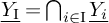 . If we denote by
$\mathrm {I}^c:= \Delta ^n\setminus \mathrm {I}$
 , there are isomorphisms

obtained by deleting redundant coordinates, which induces a log structure on
$\underline {Y_{\mathrm {I}}}$
 .
For
$i \in \mathbb {N}$
 , we define

and we denote by
$(X^n,Y^{\bullet })$
 the family thus defined. Note that for
$i>0$
 , there are i natural morphisms

given by the diagram for
$\mathrm {I} \subsetneq \{0,\dots ,n\}$
 , and
$k \in \mathrm {I}$


where the right morphism is the k-th coface of
$\mkern1mu_{\mathbf {x}}\mathrm {P}_{\mathbf {y}}X$
 .
These morphisms endow
$(X^n,Y^{\bullet })$
 with a natural structure of an augmented symmetric semi-simplicial object in
$\!^{\mathbf {v}}\mathbf {Div}_k$
 , that is a diagram in
$\!^{\mathbf {v}}\mathbf {Div}_k$
 indexed by the category of finite sets, with injective morphisms between them (see [Reference Chan, Galatius and PayneCGP21, Section 3]).
Definition 5.2.15. We let
$\boldsymbol {\Gamma }_{\mathrm {B}}(X^n,Y^{\bullet })$
 be the complex in
$\mathcal {M}\mathrm {od}_{\mathbb {Q}}$
 associated with the augmented symmetric semi-simplicial variety with log corners
$(X^n,Y^{\bullet })$
 after applying
$\boldsymbol {\Gamma }_{\mathrm {B}}^\otimes $
 .
Remark 5.2.16. If we denote by
$Y:= \cup _i Y_i$
 , then it is a classical fact (see [Reference Deligne and GoncharovDG05]) that the complex
$\boldsymbol {\Gamma }_{\mathrm {B}}(X^n,Y^{\bullet })$
 is closely related to the relative Betti cohomology of the pair
$(X^n,Y)$
 , that we denote by
$\boldsymbol {\Gamma }_{\mathrm {B}}(X^n,Y)$
 . More precisely, there is a fibre sequence

where
$Y_{\Delta ^n} := \cap _{i\in \{0,\dots ,n\}} Y_i$
 . Note that it is either a point if
$\mathbf {x} = \mathbf {y}$
 , or the empty set if
$\mathbf {x} \neq \mathbf {y}$
 . Hence the fibre sequence induces an isomorphism

when
$\mathbf {x} \neq \mathbf {y}$
 .
In general, the complex
$\boldsymbol {\Gamma }_{\mathrm {B}}(X^n,Y^{\bullet })$
 is used to compute the filtered pieces of the bar construction. Indeed, with [Reference Ignacio Burgos Gil and FresánBGF25, 3.297, Lemma 3.298] we know that there are natural quasi-isomorphisms of complexes

The quasi-isomorphisms can be described this way: The complex
$\boldsymbol {\Gamma }_{\mathrm {B}}(X^n,Y^{\bullet })$
 can be represented by the total complex of the double complex

where the horizontal differentials are given by the semi-simplicial structure of
$(X^n,Y^{\bullet })$
 (see a full description in [Reference Ignacio Burgos Gil and FresánBGF25, A.8.3]).
The complex
$\boldsymbol {\Gamma }_{\mathrm {B}}(\mkern1mu^{}_{\mathbf {x}}\mathrm {P}^{\bullet }_{\mathbf {y}}X_{\leq n})$
 is obtained as the total complex of the double complex

where the horizontal differentials are given by the cosimplicial structure of
$\mkern1mu^{}_{\mathbf {x}}\mathrm {P}^{\bullet }_{\mathbf {y}}X^{\mathrm {KN}}$
 .
The complexes (5) and (6) are isomorphic up to a shift of degree n, and the isomorphism is given explicitly in degree k by:

where
$(\omega _{\mathrm {I}})$
 is defined by

where we let
$\epsilon (\mathrm {I}):= \prod _{i \in \mathrm {I}} (-1)^i$
 , and where
$\omega _i = \omega _{|\mathrm {I}^c|-1}$
 as a cochain on
$(X^{\mathrm {KN}})^{|\mathrm {I}^c|-1}$
 , is viewed as a cochain on
$Y_{\mathrm {I}}^{\mathrm {KN}}$
 .
Remark 5.2.17. The signs appearing above are conventions, and they are constrained by the signs chosen for the differentials of the complexes involved. We followed here the conventions from [Reference Ignacio Burgos Gil and FresánBGF25].
Using this representation, the isomorphism given by the Beilinson lemma is classically described as follows:
For
$i\in \mathbb {N}$
 , let us denote by

the standard i-simplex. Let
$\gamma : [0,1] \rightarrow X^{\mathrm {KN}}$
 be a continuous path based at
$\mathbf {x},\mathbf {y}$
 . It induces a singular chain

Moreover, for
$\mathrm {I} \subsetneq \{0,\dots , n \}$
 ,
$\sigma _{\gamma ,|\mathrm {I}^c|-1}$
 defines a map

Proposition 5.2.18 [Reference Deligne and GoncharovDG05, Example 3.8],[Reference Ignacio Burgos Gil and FresánBGF25, Section 3.6.4]
The isomorphism

where J is defined as in Remark 5.2.12, is dual to the map obtained via

Remark 5.2.19. The signs are again conventions fixed in a coherent way with the conventions chosen above.
5.3 The de Rham realization
5.3.1 The de Rham fundamental groupoid at tangential basepoints
We now give a definition of the de Rham fundamental torsor at tangential basepoints, and compare it with the de Rham realization of the motivic pointed path space based at tangential basepoints. We suppose k of characteristic
$0$
 in this section. Let us take again
$X\in \mathbf {Div}_k$
 , with tangential basepoints
$\mathbf {x},\mathbf {y}$
 . We will emphasize the point of view, taken from section 2, on
$\mathbf {x},\mathbf {y}$
 as virtual morphisms
$* \rightarrow X$
 .
Recall that the sheaf of log de Rham differentials
$\Omega ^1_{-/k}$
 is functorial with respect to virtual morphism with reduced source [Reference Dupont, Panzer and PymDPP24, Lemma 5.9]. Therefore the log de Rham cohomology
$\textbf {R}\Gamma (X,\Omega _{X/k}) \in \operatorname {\mathrm {CAlg}}(\mathcal {M}\mathrm {od}_k)$
 comes with canonical augmentations defined by functoriality

Definition 5.3.1. The de Rham path space of X based at
$\mathbf {x},\mathbf {y}$
 is defined by

The de Rham fundamental torsor at
$\mathbf {x},\mathbf {y}$
 of X is defined by

Remark 5.3.2. As before, it follows from theorem 4.1.9, that the family
$\{\mkern1mu^{}_{\mathbf {x}}\mathrm {P}^{\mathrm {dR}}_{\mathbf {y}}X\}_{\mathbf {x},\mathbf {y}}$
 is endowed with the structure of a homotopy Hopf algebroid, so that the family
$\{\pi ^{\text {dR}}_1(X,\mathbf {x},\mathbf {y})\}_{\mathbf {x},\mathbf {y}}$
 has the structure of a groupoid. We call it the
de Rham fundamental groupoid.
5.3.2 The de Rham realization functor
We can now move to the identification of the de Rham realization of the motivic pointed path space based at tangential basepoints. Let us first build the log de Rham realization functor.
Proposition 5.3.3. There exists a log de Rham realization functor

such that for
$X \in \mathbf {lSm}_k$
 , there is a natural equivalence

and such that the following diagram commutes:

Definition 5.3.4. The log de Rham
$\mathcal {M}\mathrm {od}_k$
 -valued log mixed Weil theory over k is the symmetric monoidal functor

This indeed defines a symmetric monoidal
$\infty $
 -functor: from [Reference Blumberg, Gepner and TabuadaBGT14, Proposition 3.5], we see that it suffices to show that the functor of 1-categories

where
$\mathbf {R}\Gamma (-,\Omega _{-/k})$
 denotes by an abuse of notation a symmetric monoidal resolution of complexes of sheaves functor (e.g. the Thom-Whitney normalization of the Godement resolution [Reference Navarro AznarAzn87]) is such that
-
• it is lax symmetric monoidal,
-
• $k \rightarrow \boldsymbol {\Gamma }(\mathrm {Spec}(k))$
is a quasi-isomorphism, -
• $\boldsymbol {\Gamma }(X) \otimes \boldsymbol {\Gamma }(Y) \rightarrow \boldsymbol {\Gamma }(X\times Y)$
is a quasi-isomorphism for all
$X,Y \in \mathbf {lSm}_k.$


These conditions are straightforward properties of the log de Rham cohomology. The proposition cited above defines a symmetric monoidal functor of
$\infty $
 -categories.
Proof of proposition 5.3.3
The functor
$\boldsymbol {\Gamma }_{\operatorname {dR}}$
 is
$\text {ver}$
 -invariant by [Reference OgusOgu18, Proposition V.4.2.5], hence it satisfies
$\mathrm {dNis}$
 -descent (
$\omega : X \mapsto X\setminus \partial X$
 sends
$\mathrm {dNis}$
 covers to
$\mathrm {Nis}$
 covers) since the classical de Rham cohomology satisfies Nisnevich descent. Moreover,
$\boldsymbol {\Gamma }_{\mathrm {dR}}(\mathbb {G}_m^{\mathrm {log}}) \simeq \boldsymbol {\Gamma }_{\mathrm {dR}}(\mathbb {G}_m)$
 so that it sends
$\mathbb {G}^{\mathrm {log}}_m/1$
 on a
$\otimes $
 -invertible object, and naturally
$ \boldsymbol {\Gamma }_{\mathrm {dR}}(\mathbb {A}^1)\simeq k$
 .
Finally, it takes values in
$\mathrm {Perf}(k)$
 since the de Rham cohomology has finite dimension.
Remark 5.3.5. Since the log de Rham cohomology of the log point
$*_{\mathbb {N}}$
 and of the log scheme
$\mathbb {A}_{\mathbb {N}}$
 are computed by applying the functor of global sections of the corresponding log de Rham complexes, it is easy to see that the morphism

is an equivalence.
5.3.3 Computation of the de Rham realization of the motivic fundamental groupoid
Let us now compute the realization of the motivic pointed path space:
Theorem 5.3.6. Let
$X\in \mathbf {Div}_k.$
 For
$\mathbf {x}, \mathbf {y}$
 tangential basepoints on X, there is a natural equivalence

In particular, when X is such that
$M(X)$
 is a mixed Tate motive, there is a natural isomorphism of groupoids induced by

Proof. Once again, using the fact that
$\mathrm {R}_{\mathrm {dR}}$
 is colimit preserving, it commutes with the bar construction, so that

Now, the morphism
$\mathrm {R}_{\mathrm {dR}}(\mathbf {x})$
 (similarly for
$\mathrm {R}_{\mathrm {dR}}(\mathbf {y})$
 ) is defined after the choice of a homotopy inverse to the equivalence

Such a homotopy equivalence is found by functoriality applied to the virtual retraction

which is defined trivially on the underlying schemes, and by the obvious morphism of sheaves in monoids

(note that this is indeed a retraction of the natural morphism
$-^{\mathrm {log}} \rightarrow \mathrm {N}_{\mathbf {x}}^{\mathrm {log}}(X,D)$
 ) so that the composition

is nothing but the virtual morphism defining
$h(\mathbf {x}),h(\mathbf {y})$
 . This concludes the proof.
Arguing as in the previous subsection, we see that the de Rham path space can be canonically obtained from the cosimplicial log scheme introduced in subsubsection 4.2.1

after applying the functor
$\textbf {R}\Gamma (-,\Omega _{-/k})$
 and taking the associated total complex.
As in the Betti case, we can go a little further and give a more detailed description of the de Rham fundamental groupoid after extension of the scalar to
$\mathbb {C}$
 . In order to compute the periods of the motivic fundamental groupoid in the next sections, we interpret the de Rham fundamental groupoid via the de Rham theory of manifolds with log corners.
Recall from [Reference Dupont, Panzer and PymDPP23] that a manifold with log corners
$(\Sigma ,\mathcal {M}_\Sigma )$
 is a manifold with corners
$\underline {\Sigma }$
 endowed with a positive log structure (this notion is developed in [Reference Gillam and MolchoGM15]): a sheaf of monoids
$\mathcal {M}_\Sigma $
 on
$\underline {\Sigma }$
 and a morphism
$\alpha : \mathcal {M}_\Sigma \rightarrow \mathcal {C}^{\infty ,\geq 0}_\Sigma $
 where
$\mathcal {C}^{\infty ,\geq 0}_\Sigma $
 is the sheaf of non-negative smooth functions on
$\underline {\Sigma }$
 , with the property that it induces an isomorphism
$\alpha ^{-1}(\mathcal {C}^{\infty ,> 0}_\Sigma ) \xrightarrow {\sim } \mathcal {C}^{\infty ,> 0}_\Sigma $
 . We furthermore ask X to be locally isomorphic (as a manifold with corners equipped with a positive log structure) to an open subset of the standard corner
$[0)^k\times [0,\infty )^n$
 .
The latter is defined by the underlying manifold with corners
$\{0\}^k\times [0,\infty )^n \subset [0,\infty )^{n+k}$
 equipped with the sheaf

where the
$r_i$
 are coordinates on
$[0,\infty )^n$
 and the
$t_i$
 are formal ‘phantom’ coordinates evaluated to
$0$
 in
$\mathcal {C}^{\infty ,\geq 0}_{[0,\infty )^n}.$
 See [Reference Dupont, Panzer and PymDPP23, Section 3.2] for details. A manifold with log corners is locally obtained as the restriction at a closed submanifold with corners of the manifold with log corners
$[0,\infty )^n$
 for a non-negative integer n (e.g.
$[0) \times [0,\infty )$
 is obtained as the restriction of the positive log structure
$[0,\infty )^2$
 on the line
$r_1 = 0$
 . The coordinate
$r_1$
 is turned into the phantom coordinate
$t_1$
 ).
Example 5.3.7.
-
• The manifold with corners $[0,\infty )$
with coordinate r is equipped with the structure of a manifold with log corners via the positive log structure $$ \begin{align*}\alpha: \mathcal{C}^{\infty,>0}_{[0,\infty)}r^{\mathbb{N}} \hookrightarrow \mathcal{C}^{\infty,\geq 0}_{[0,\infty)}.\end{align*} $$
-
• The Kato–Nakayama space of the log scheme $\mathbb {A}_{\mathbb {N}}$
is the oriented real blow-up of
$\mathbb {R}^2$
at
$0$
. It is then endowed with the structure of a manifold with log corners
$S^1 \times [0,\infty )$
where
$S^1$
is endowed with the trivial positive log structure.


In general, for
$X\in \mathbf {Div}_k$
 ,
$X^{\mathrm {KN}}$
 has the structure of a manifold with log corners [Reference Dupont, Panzer and PymDPP23, Proposition 8.4], and virtual points
$* \rightarrow X$
 define virtual points of
$X^{\mathrm {KN}}$
 , that is virtual morphisms in the sense of [Reference Dupont, Panzer and PymDPP23, Definition 4.1] (the definition is similar to definition 2.2.1). Such a virtual point keeps track of the whole datum of the tangential basepoint, not only its direction, so that when X is defined over
$\mathbb {C}$
 , there is a bijection between tangential basepoints of X and virtual points of
$X^{\mathrm {KN}}$
 [Reference Dupont, Panzer and PymDPP23, Proposition 8.8]. Hence, this fills the gap between tangential basepoints on X, and points on
$X^{\mathrm {KN}}$
 explained at the end of subsection 2.2.
Example 5.3.8. A virtual morphism from the point to
$\mathbb {A_N}^{\mathrm {KN}}$
 landing on the infinitesimal unit circle at
$0$
 is the same as the choice of a direction u and of the pullback of the phantom coordinate t associated with
$r = 0$
 in
$\mathcal {C}^{\infty ,>0}_* \simeq \mathbb {R}_+^*$
 . The last datum allows to differentiate between tangential basepoints induced by
$\lambda $
 or
$a\lambda $
 for a a strictly positive constant, see example 2.2.5.
A manifold with log corners
$\Sigma $
 is endowed with a de Rham complex of logarithmic differential forms
$\mathcal {A}_\Sigma $
 , functorial with respect to virtual morphisms [Reference Dupont, Panzer and PymDPP23, Section 6.2], which adds to the complex of classical differential forms, formal logarithmic differential forms
$\mathrm {dlog}(r_i),\mathrm {dlog}(t_j)$
 . This construction is similar to the construction of the algebraic logarithmic de Rham complex so that for
$X \in \mathbf {Div}_k$
 there are canonical quasi-isomorphisms, see [Reference Dupont, Panzer and PymDPP23, Sections 8.5,6]:

where we denoted by
$\mathcal {A}(\Sigma ):= \Gamma (\Sigma ,\mathcal {A}_\Sigma )$
 . In particular, for
$\mathbf {x,y}$
 tangential basepoints on X, the de Rham path space based at
$\mathbf {x},\mathbf {y}$
 satisfies

where
$\mathbf {x},\mathbf {y}$
 are viewed as virtual morphisms
$*\rightarrow X^{\mathrm {KN}}$
 .
Note that
$\mathcal {A}(X^{\mathrm {KN}})$
 is a commutative differential graded algebra, so that we can use the description from example 4.1.13:
$\;_{\mathbf {x}}\mathrm {Bar}_{\mathbf {y}}(\mathcal {A}(X^{\mathrm {KN}}))$
 is interpreted as a complex of formal iterated integrals; its elements are denoted by

in degree
$\sum _i n_i - k$
 , and the differentials are described for instance in [Reference Ignacio Burgos Gil and FresánBGF25, 3.250].
The equivalence above can be refined at the filtered level:

The complex on the right is the subcomplex
$\mkern1mu_{\mathbf {x}}\mathrm {Bar}_{\mathbf {y}}(\mathcal {A}(X^{\mathrm {KN}})) \otimes _{\mathbb {R}} \mathbb {C}$
 spanned by elements
$[\omega _1|\dots | \omega _k]$
 with
$k \leq n$
 . As before, we can see that there is an isomorphism of complexes

We will use in the following subsections the description of this isomorphism in [Reference Ignacio Burgos Gil and FresánBGF25, 3.284] that we specialize into the following:
Lemma 5.3.9. The isomorphism is given by

where

Remark 5.3.10. For
$[\omega _1|\dots |\omega _k] \in \mkern1mu_{\mathbf {x}}\mathrm {Bar}_{\mathbf {y}}(\mathcal {A}(X^{\mathrm {KN}}))_{\leq n}$
 with
$k\leq n$
 and
$\deg (\omega _i) = 1$
 , we see that the outcome of the previous isomorphism is
$(-1)^{\frac {k(k-1)}{2}}\mathrm {pr}_1^*\omega _1 \wedge \cdots \wedge \mathrm {pr}_k^*\omega _k$
 in position k.
5.4 The comparison isomorphism
We now describe the Betti–de Rham comparison isomorphism applied to the motivic pointed path space based at tangential basepoints. This will allow us in the next subsection to compute the periods of the motivic fundamental groupoid at tangential basepoints. Let us remind that the log Betti and log de Rham cohomologies are, as in the classical setting, compared in a canonical way by the work of Kato and Nakayama [Reference Kato and NakayamaKN99]. Namely, for X an ideally log smooth log scheme over k, there is a natural isomorphism

Remark 5.4.1. The definition of ideally log smooth log schemes over a field k, as given in [Reference OgusOgu18], characterizes log schemes étale locally modelled on
$\mathrm {Spec}(k[P]/(\Sigma ))$
 where P is an fs monoid, and
$(\Sigma )$
 is the ideal of
$k[P]$
 generated by an ideal
$\Sigma $
 of P. This definition includes in particular the standard log point
$*_{\mathbb {N}} \simeq \mathrm {Spec}(k[\mathbb {N}]/(\mathbb {N}^+))$
 .
The comparison theorem refines into:
Theorem 5.4.2. For
$\Lambda $
 a subring of
$\mathbb {C}$
 , there is an equivalence of symmetric monoidal
$\infty $
 -functors

Proof. By the result of lemma 5.1.5, to prove the theorem it suffices to compare the associated log mixed Weil theories. Note that by the construction of these functors and after [Reference Blumberg, Gepner and TabuadaBGT14, Proposition 3.5], we only need to compare the associated functors of
$1$
 -categories

The log Betti-log de Rham comparison theorem [Reference Kato and NakayamaKN99, 0.2] gives a weak equivalence of lax monoidal functors

which directly shows the expected result.
It then suffices to apply the Betti–de Rham comparison to the motivic pointed path space to see that for
$X\in \mathbf {Div}_k$
 , and
$\mathbf {x,y}$
 tangential basepoints on X, there are natural isomorphisms of schemes compatible with the groupoid structure

The only thing that needs to be checked is that the Betti and de Rham realizations of the motivic augmentations associated with
$\mathbf {x}$
 and
$\mathbf {y}$
 are naturally isomorphic. This is trivial using remark 5.4.1 and lemma 5.1.7.
This result can be refined by applying the Betti–de Rham comparison to the filtered pieces of the motivic pointed path space to obtain an isomorphism of k-algebras for all
$n\in \mathbb {N}$


.
Recall now that for
$\Sigma $
 a manifold with log corners (see the end of subsection 5.3), its de Rham and singular cohomologies are compared via a log Poincaré lemma. Namely, the canonical inclusion of complex of sheaves
$\Sigma $


is a quasi-isomorphism, see [Reference Dupont, Panzer and PymDPP23, Corollary 6.9]. This is compatible with the algebraic log de Rham, log Betti comparison theorem in the sense that for
$X\in \mathbf {Div}_k$
 , the comparison isomorphism between its log de Rham and log Betti cohomologies is given after tensoring by
$\mathbb {C}$
 the quasi-isomorphism

in a natural way. From the descriptions at the end of the last two sections, we see that the filtered comparison isomorphism applied to the motivic path space based at
$\mathbf {x},\mathbf {y}$
 is given after tensoring by
$\mathbb {C}$
 and taking the
$0$
 -th homology on the following quasi-isomorphism of complexes:

5.5 Periods of the motivic fundamental groupoid
With the previous interpretation of the comparison isomorphism, we can now compute the periods of the motivic fundamental groupoid at tangential basepoints via regularized integration. This will allow us to prove in general a variant of Chen’s theorem (see theorem 5.5.10) for tangential basepoints relating the prounipotent completion of the fundamental group with the right notion of iterated integrals. In this last subsection,
$k \subset \mathbb {C}$
 .
5.5.1 Regularized integration
Let us first recall some facts on regularized integrals introduced in full generality in [Reference Dupont, Panzer and PymDPP23]. We refer the reader to the introduction to positive log geometry at the end of subsection 5.3.
For
$\Sigma $
 a manifold with log corners and for
$i> 0$
 , we denote by
$\partial ^i\Sigma $
 , and we call i-th boundary of
$\Sigma $
 the manifold with log corners described locally by iterating on the following

We omit the i in the notation
$\partial ^i\Sigma $
 when
$i = 1$
 , and we let
$\partial ^0 \Sigma := \Sigma $
 .
If
$i>0$
 , there are i natural ordinary morphisms of manifolds with log corners

This way, the family
$(\Sigma , \partial ^{\bullet }\Sigma )$
 defines an augmented symmetric semi-simplicial manifold with log corners, as defined in the discussion introducing the definition 5.2.15.
Example 5.5.1. The topological n-simplex
$\Delta ^n$
 (with the model described in 7) is endowed with the structure of a manifold with corners hence of a manifold with log corners. Recall that one needs to be careful in the choice of the associated positive log structure. It is not true in general that, when equipped with the trivial positive log structure
$\mathcal {C}^{\infty ,>0}_\Sigma $
 , a manifold with corners
$\Sigma $
 is a manifold with log corners. We can instead use [Reference Dupont, Panzer and PymDPP23, Section 3.2.3] where the choice consists in pulling back the positive log structures on each local chart
$U \rightarrow [0,\infty )^n$
 .
-
• When $n = 2$
, the boundary of
$\Delta ^2$
can be described in a simple way as the disjoint union of its faces, each isomorphic as manifold with log corners to
$\Delta ^1\times [0)$
. The picture in this case is: The second boundary $\partial ^2\Delta ^2$
is a disjoint union of two copies of each vertex of
$\Delta ^2$
endowed with the positive log structure
$[0)^2$
. The two rightmost morphisms are the natural immersion, and the morphism deduced via the action of the symmetric group
$\mathfrak {S}_2$
with exchanges copies of the same vertex. Note that
$\partial ^i \Delta ^2$
is empty for
$i> 2$
. -
• In general, $\partial ^i\Delta ^n$
is a disjoint union of
$i!$
copies of each
$(n-i)$
-dimensional face in
$\Delta ^n$
, and there is an action of the symmetric group
$\mathfrak {S}_i$
permuting them.


For
$\Sigma $
 a manifold with log corners, we can consider the associated basic manifold with log corners
$\Sigma ^{\mathrm {bas}}$
 , defined locally by the property that

In other words, the underlying manifolds with log corners of
$\Sigma $
 and its basic version are the same, and the positive log structure of
$\Sigma ^{\mathrm {bas}}$
 is obtained from the original on
$\Sigma $
 by restricting to the submonoid of functions whose germ at each point of
$\Sigma $
 is not sent to zero by the germ of the morphism
$\mathcal {M}_\Sigma \rightarrow \mathcal {C}_\Sigma ^{\infty ,\geq 0}.$
 There is a morphism of manifolds with log corners

induced by the inclusion
$\mathcal {M}_{\Sigma ^{\mathrm {bas}}}\hookrightarrow \mathcal {M}_{\Sigma }.$
 We say that
$\Sigma $
 is basic if
$\Sigma ^{\mathrm {bas}} \simeq \Sigma $
 .
In [Reference Ignacio Burgos Gil and FresánBGF25, Section 3.8.6], the definition of the regularized integral of a differential form on the projective line with logarithmic poles at
$\{0,1,\infty \}$
 is based on the choice of tangential basepoints at these points. Indeed, it is defined [Reference Ignacio Burgos Gil and FresánBGF25, Definition 3.364] as the residue of a logarithmic asymptotic expansion of the integral along a path whose starting and endpoints converge to removed points in the direction prescribed by the tangential datum. In higher dimension, the full definition appears in [Reference Dupont, Panzer and PymDPP23]. The choice of tangential basepoints at a finite set of points is replaced by the definition of the regularization of a manifold with log corners. Although this definition, and the definition of regularized integration work in a very general setting, we focus on the case of
$\Sigma = \Delta ^n$
 .
Definition 5.5.2. A nondegenerate regularization on
$\Delta ^n$
 is defined as a positive section of the normal bundle of the immersion of the underlying manifold with corners

This can be viewed as the datum of a family of tangential basepoints on the boundary. Tangential basepoints in this setting are defined in a similar way as in the algebraic setting, by the data of a point and of a positive normal vector at this point (outside the boundary it is just a point), see [Reference Dupont, Panzer and PymDPP23, Definition 4.8] for details.
By [Reference Dupont, Panzer and PymDPP23, Proposition 4.9], we know that there is still a bijection between tangential basepoints on a basic manifold with log corners, and virtual morphisms from the point, equipped with the trivial positive log structure.
Example 5.5.3.
-
• A virtual morphism
$$ \begin{align*}* \rightarrow [0,\infty)\end{align*} $$to $0$
is determined by the pullback
$\lambda \in \mathbb {R}_{>0}$
of the coordinate
$r \in [0,\infty )$
. As in the algebraic case, this is associated to the normal vector
$\lambda \partial _{r}|_0.$
-
• More generally, a virtual morphism
$$ \begin{align*}[0,\infty) \rightarrow [0,\infty)^2\end{align*} $$which identifies the underlying manifold with corners $[0,\infty )$
with the component
$r_2 = 0$
of the boundary of
$[0,\infty )^2$
(where we let
$(r_1,r_2)$
be coordinates for
$[0,\infty )^2$
) is the same thing as a family of tangential basepoints on the component
$r_2 = 0$
, determined by the pullback of
$r_2$
on
$\mathcal {M}_{[0,\infty )}$
. Note that this datum is equivalent to the datum of a virtual morphism $$ \begin{align*}[0,\infty) \simeq ([0,\infty)\times [0))^{\mathrm{bas}} \rightarrow [0,\infty)\times [0),\end{align*} $$which is a section of the morphism $[0,\infty )\times [0) \rightarrow ([0,\infty )\times [0))^{\mathrm {bas}}$
and where the tangential datum is now given by the pullback of the phantom coordinate
$t_2.$




In the same fashion as this last example, if we let
$\partial _i\Delta ^n$
 be the i-th face of
$\Delta ^n$
 with the induced positive log structure, a family of positive normal vectors to
$\underline {\partial _i\Delta }^n$
 in
$\underline {\Delta }^n$
 is the same as the datum of a section

to the morphism
$\partial _i\Delta ^n \rightarrow (\partial _i\Delta ^n)^{\mathrm {bas}}$
 , the normal vector being determined by the pullback of the coordinate vanishing on the face
$\partial _i\Delta ^n$
 to
$\mathcal {M}_{(\partial _i\Delta ^n)^{\mathrm {bas}}}$
 (
$t_{i+1}-t_i$
 if
$0 < i <n$
 ,
$t_0-1$
 if
$i = 0$
 and
$t_n$
 if
$i = n$
 ).
Therefore, there is a commutative diagram of manifolds with log corners

More generally, it is explained in [Reference Dupont, Panzer and PymDPP23, Proposition 7.4], that the datum of a nondegenerate regularization s of
$\Delta ^n$
 induces, by pulling back s along all the k different immersions
$\underline {\partial ^k \Delta ^n} \hookrightarrow \underline {\partial \Delta ^n}$
 a family of positive normal vectors on to
$\underline {\partial ^k \Delta ^n}$
 , and hence a section

The data of these sections for
$k \in \mathbb {N}$
 induces in a unique way a structure of augmented symmetric simplicial manifold with log corners, with virtual morphisms,
$((\Delta ^n)^{\mathrm {bas}},(\partial ^{\bullet }\Delta ^n)^{\mathrm {bas}})$
 (note that the operation
$-^{\mathrm {bas}}$
 is not functorial, see for instance the inclusion
$[0) \hookrightarrow [0,\infty )$
 ), and a morphism of augmented symmetric semi-simplicial manifolds with log corners

We refer the reader to [Reference Dupont, Panzer and PymDPP23, Subsection 7.1] for details. Note that we will not need to describe explicitly the structure of augmented symmetric semi-simplicial manifolds with log corners of
$((\Delta ^n)^{\mathrm {bas}},(\partial ^{\bullet }\Delta ^n)^{\mathrm {bas}})$
 .
Definition 5.5.4. Let us consider the section of the normal bundle of the immersion
$\underline {\partial \Delta }^n \hookrightarrow \underline {\Delta }^n$
 obtained as
-
• $-\frac {\partial }{\partial t_1}\big |_{\underline {\partial _1\Delta }^n}$
on
$\underline {\partial _1\Delta }^n$
, -
• $(\frac {\partial }{\partial t_i} -\frac {\partial }{\partial t_{i+1}})\big |_{\underline {\partial _i\Delta }^n}$
on
$\underline {\partial _i\Delta }^n$
if
$0 <i <n$
, -
• $\frac {\partial }{\partial t_n}\big |_{\underline {\partial _n\Delta }^n}$
on
$\underline {\partial _n\Delta }^n$
.


We denote by

the induced morphism of augmented symmetric semi-simplicial manifolds with log corners where we made implicit the structure of augmented symmetric semi-simplicial manifold with log corners of
$((\Delta ^n)^{\mathrm {bas}},(\partial \Delta ^n)^{\mathrm {bas}})$
 .
With this regularization at hand, for
$\omega \in \mathcal {A}^{n}(\Delta ^n)$
 a logarithmic differential form on
$\Delta ^n$
 , the regularized integral of
$\omega $
 on
$\Delta ^n$
 denoted by

is defined as the classical integral of the cohomology class
$[s^*\omega ]$
 in

on
$\underline {\Delta }^n$
 . More generally, for
$(X,Y^{\bullet })$
 an augmented symmetric semi-simplicial manifold with log corners, and
$\omega \in \mathcal {A}^n(X)$
 a logarithmic differential form of degree n vanishing on
$Y^{\mathbf {1}}$
 , if there is a morphism

of symmetric semi-simplicial manifolds with log corners, then the regularized integral of
$\omega $
 on
$\phi $
 is defined by

By functoriality of the Betti-de Rham comparison theorem for manifolds with log corners (see the end of the subsection 5.4), we have

via the pairing

see [Reference Dupont, Panzer and PymDPP23, Proposition 8.11].
5.5.2 Regularized iterated integration
Let us now compute the periods of the motivic fundamental groupoid in terms of regularized iterated integrals. We first define this notion in definition 5.5.8. Let
$X \in \mathbf {Div}_k$
 and
$\mathbf {x},\mathbf {y}$
 tangential basepoints on X.
Let
$\gamma :\, (0,1)\, \rightarrow \underline {X}(\mathbb {C})\setminus \underline {D}(\mathbb {C})$
 be a smooth path of
$\underline {X}(\mathbb {C})\setminus \underline {D}(\mathbb {C})$
 based at the tangential basepoints
$\mathbf {x},\mathbf {y}$
 (definition 5.2.3). Recall that since
$\gamma $
 can be continuously extended to a map
$[0,1] \rightarrow X^{\mathrm {KN}}$
 , we can define a continuous map

for
$i \in \mathbb {N}$
 as in the discussion following remark 5.2.17.
Remark 5.5.5. Since
$\gamma $
 is smooth, it induces a morphism of manifolds with corners
$[0,1] \rightarrow X^{\mathrm {KN}}$
 . In coordinates, locally around
$\mathbf {x}$
 or
$\mathbf {y}$
 ,
$X^{\mathrm {KN}} \simeq (\mathbb {R}_{+}\times S^1)^p\times (\mathbb {R}_+^{*})^{q}$
 so that locally around
$0$
 for instance,
$\gamma (t) = (r_1(t), \theta _1(t), \dots , r_p(t),\theta _p(t), x^{\prime }_1(t), \dots , x^{\prime }_{q}(t))$
 and
$r_i$
 satisfies
$r_i(t) \sim _0 t\lambda _i$
 with
$\lambda _i> 0$
 . Therefore, using the condition specified in the discussion following [Reference Dupont, Panzer and PymDPP23, Definition 3.14], we see that
$\gamma $
 is uniquely lifted into an ordinary morphism of manifolds with log corners

More generally the following lemma is proven in the same fashion working locally in coordinates:
Lemma 5.5.6. For
$i \in \mathbb {N}$
 and under the hypotheses on
$\gamma $
 , the map
$\sigma _{\gamma ,i}$
 has the structure of an ordinary morphism of manifolds with log corners.
The following proposition will allow us to define regularized iterated integration. Recall that we defined at the end of subsection 5.2 an augmented symmetric semi-simplicial object in
$\!^{\mathbf {v}}\mathbf {Div}_k$
 denoted by
$(X^k,Y^{\bullet }).$
 Since the Kato-Nakayama space is functorial with respect to virtual morphisms, this defines an augmented symmetric semi-simplicial manifold with log corners (with virtual morphisms between the objects)
$((X^{\mathrm {KN}})^k,(Y^{\bullet })^{\mathrm {KN}})$
 .
Proposition 5.5.7. For
$\gamma $
 defined as above,
$\sigma _{\gamma ,k}$
 defines an ordinary morphism of augmented symmetric semi-simplicial manifolds with log corners

First, note that since for
$0 \leq i \leq k$
 , the i-th face of the standard k-simplex is given by
-
• $\{t_1 = 1\}$
if
$i = 0$
-
• $\{t_i = t_{i+1} \}$
if
$0 < i < k $
-
• $\{t_k = 0\}$
if
$i = k$


we remark that
$\sigma _{\gamma ,k}$
 induces a morphism of manifolds with corners

This map induces a morphism of manifolds with log corners by the following identification

Iterating this construction, we see that for
$\mathrm {I} = (i_1,\dots , i_j) \subset [k]$
 with
$i_1 < \dots < i_k$
 ,
$\sigma _{\gamma ,k}$
 induces by restriction a morphism of manifolds with log corners

identified with the morphism
$\sigma _{\gamma ,k-j}.$

Therefore, there is a diagram of manifold with log corners

such that the underlying diagram of manifolds with corners commutes. Let us prove the proposition 5.5.7.
Proof. We can work by induction on k. When
$k = 0$
 nothing needs to be done.
Suppose that the statement is true for
$k - 1 \geq 0$
 . Then we only need to show that the following square of manifolds with log corners commutes

We work on each face separately, we wish to show that for
$0 \leq i \leq k$
 , the diagram

commutes. Note that by the so-called ‘continuity principle’ [Reference Dupont, Panzer and PymDPP23, Proposition 4.3], we only need to check that for each section of
$\mathcal {M}_{(X^k)^{\mathrm {KN}}}$
 pulled back to the zero function in
$\mathcal {C}^{\infty ,\geq 0}_{(\partial _i \Delta ^k)^{\mathrm {bas}}}$
 by the down-left composition

its pull back in
$\mathcal {M}_{(\partial _i \Delta ^k)^{\mathrm {bas}}}$
 by f and by the upper right composition

coincide. The rest of the sections behave according to the morphism of manifolds with corners structure.
-
• If $0 < i < k$
, by working locally in coordinates we see that no sections of
$\mathcal {M}_{(X^k)^{\mathrm {KN}}}$
are pulled back to the zero section by f. -
• If $i = k$
, then
$(\partial _i \Delta ^k)^{\mathrm {bas}} = \{t_1 = 0\}^{\mathrm {bas}}$
so that
$\sigma _{\gamma ,k}$
when restricted is the morphism $$ \begin{align*}(t_1 = 0,t_2, \dots, t_k) \rightarrow (\mathbf{x},\gamma(t_2),\dots, \gamma(t_k)).\end{align*} $$
In coordinates, close to $\{\mathbf {x}\}\times (X^{k-1})^{\mathrm {KN}}$
(we use the same coordinates as in the remark 5.5.5), we can write in a neighbourhood of
$t_1 = 0$
$$ \begin{align*}\sigma_{\gamma,k}(t_1,\dots,t_k) = (r_1(t_1), \theta_1(t_1), \dots, r_p(t_1),\theta_p(t_1), x^{\prime}_1(t_1), \dots, x^{\prime}_{q}(t_1), \gamma(t_2),\dots,\gamma(t_k))\end{align*} $$
we then see clearly that the only coordinates pulled back on the zero section are $r_1,\dots , r_p$
.Let $\lambda _i:= \mathbf {x}^*r_i$
. On one hand we see that
$\sigma _{\gamma ,k}^*r_i = \lambda _i$
, which readily shows that
$g^*r_i = \lambda _i$
. On the other hand, since
$\gamma $
is a path based at the tangential basepoint
$\mathbf {x}$
at zero, we have that
$r^{\prime }_i(0) = \lambda _i$
. The pullback of
$r_i$
in
$\mathcal {M}_{(Y_i)^{\mathrm {KN}}}$
by the morphism
$Y_i \rightarrow (X^k)^{\mathrm {KN}}$
is
$r_i(t_1)$
, and the pullback of
$r_i(t_1)$
by the virtual morphism
$(\partial _i\Delta ^k)^{\mathrm {bas}} \rightarrow \Delta ^k$
in
$\mathcal {M}_{(\partial _i\Delta ^k)^{\mathrm {bas}}}$
is
$r_i'(0)$
since this morphism is determined by the virtual morphism
$\partial _{t_1 = 0}$
by the choice of the section of the normal bundle. Hence the result. -
• If $r'_i(0)$
the situation is the same as the previous one.


We can then make the following definition:
Definition 5.5.8. Let
$X\in \mathbf {Div}_k$
 ,
$\mathbf {x},\mathbf {y}$
 tangential basepoints on X, and
$\gamma : \,(0,1)\, \rightarrow \underline {X}(\mathbb {C})\setminus \underline {D}(\mathbb {C})$
 a smooth path of
$\underline {X}(\mathbb {C})\setminus \underline {D}(\mathbb {C})$
 based at
$\mathbf {x},\mathbf {y}$
 . Let
$\omega _1,\dots ,\omega _k$
 be logarithmic differential
$1$
 -forms. We define

the regularized iterated integral of
$\omega _1,\dots ,\omega _k$
 along
$\gamma $
 .
Remark 5.5.9. When
$\omega _1,\dots ,\omega _k$
 are smooth forms of the manifold with corners
$\underline {X^{\mathrm {KN}}}$
 (for instance for smooth algebraic forms), we know from [Reference Dupont, Panzer and PymDPP23, Proposition 7.2] that this definition coincides with the usual definition of iterated integral introduced by Chen, see [Reference ChenChe77]. This is true in particular when
$\mathbf {x}, \mathbf {y}$
 are rational basepoints of
$\underline {X}\setminus \underline {D}$
 .
5.5.3 The periods of the motivic fundamental groupoid
We are now able to completely determine the periods of the motivic fundamental groupoid with tangential basepoints:
Theorem 5.5.10. The isomorphism of algebras

is induced by the pairing

Proof. We can suppose X to be connected and we know that in this case every class in
$\mathrm {H}^0\big (\mkern1mu_{\mathbf {x}}\mathrm {Bar}_{\mathbf {y}}(\mathcal {A}(X^{\mathrm {KN}}))\big )$
 is represented by elements of the form
$[\omega _1| \cdots | \omega _k]$
 where the
$\omega _i$
 are
$1$
 -forms by similar arguments as [Reference Ignacio Burgos Gil and FresánBGF25, Lemma 3.263]. We have seen in subsection 5.4 (joined with the results at the end of subsections 5.3 and 5.2) that the comparison isomorphism applied to the filtered pieces of the fundamental groupoid with tangential basepoints is described by the following sequence of isomorphisms (where the upper terms are defined similarly as their Betti counterpart from the end of subsection 5.2):

For
$[\omega _1,\dots , \omega _k] \in \mkern1mu_{\mathbf {x}}\mathrm {Bar}_{\mathbf {y}}(\mathcal {A}(X^{\mathrm {KN}}))_{\leq n}$
 with
$\omega _i 1$
 -forms, its image in
$\mathcal {A}(\mkern1mu_{\mathbf {x}}\mathrm {P}_{\mathbf {y}}X^{\mathrm {KN}}_{\leq n})$
 is
$(\omega ^{\prime }_i)_{0 \leq i \leq n}$
 where

which is sent to
$(\omega ^{\prime }_{\mathrm {I}})_{\mathrm {I} \subset [n]}$
 in
$\mathcal {A}((X^{\mathrm {KN}})^n,(Y^{\bullet })^{\mathrm {KN}}) \simeq \boldsymbol {\Gamma }_{\mathrm {Sing}}((X^{\mathrm {KN}})^n,(Y^{\bullet })^{\mathrm {KN}})$
 , where

Note that the form
$\mathrm {pr}_1^*\omega _1 \wedge \cdots \wedge \mathrm {pr}_k^*\omega _k$
 restricts to
$0$
 on
$Y^{\mathbf {1}}$
 .
After the description of the isomorphism

the pairing applied to
$[\gamma ]$
 and
$[\omega _1|\dots |\omega _k]$
 is

Note that the signs cancel so that we are left with

By proposition 5.5.7, the map
$\sigma _{\gamma ,k}$
 has a structure of a morphism of augmented symmetric semi-simplicial manifolds with log corners so that

Remark 5.5.11. If we apply [Reference Dupont, Panzer and PymDPP23, Example 7.12], we can see that for
$\omega $
 an algebraic
$1$
 -form of
$\mathbb {P}^1_{\mathbb {C}}\setminus \{0,1,\infty \}$
 with logarithmic poles at
$0$
 ,
$1$
 or
$\infty $
 , then the regularized integral of
$\omega $
 along the straight path from
$0$
 to
$1$
 denoted by
$\mathbf {dch}$
 yields the same result as the regularization process defined in [Reference Ignacio Burgos Gil and FresánBGF25, Section 3.8], which consists in introducing the restricted path
$\mathbf {dch}_\eta : [\eta , 1-\eta ] \rightarrow \mathbb {P}^1_{\mathbb {C}}(\mathbb {C})\setminus \{0,1,\infty \}$
 for
$\eta \in (0,1/2)$
 and taking the residue of the logarithmic expansion of the function

More generally it is possible to prove that the regularized iterated integral

when
$\omega _i \in \{\frac {dz}{1-z},\frac {dz}{z}\}$
 yields the correct value of the corresponding regularized multiple zeta value as defined in [Reference Ignacio Burgos Gil and FresánBGF25, Section 1.7].
Acknowledgements
This article was written during my PhD at the IMAG in Montpellier with the support of the ANR Cyclades (Projet ANR-23-CE40-0011). I would like to thank my advisor, Clément Dupont, for his constant guidance and support throughout the writing process, as well as for his careful and precise comments, which allowed me to bring this article to its current form. My warmest thanks go to Swann Tubach for countless discussions on motives and six-functor formalisms, to Nikola Tomic for answering numerous questions on
$\infty $
 -categories, and to Ulysse Mounoud for our wide-ranging discussions on algebraic geometry. I also benefited from conversations with Federico Binda, Damien Calaque, Joost Nuiten and Doosung Park.
Competing interests
None declared.
Data availability statement
No data was generated or used as part of this paper.