Introduction
In the development of resilient infrastructures, structures are always affected by uncertainties from inherent natural variability, such as material properties, member sizes, and loading conditions (Kiureghian, Reference Kiureghian1989). These uncertainties are related to the physical processes that are essentially random or contain incomplete or inaccurate information. In deterministic design, these uncertainties are represented by the partial safety factor specified in design codes. This simplification, although practical, makes the values chosen for the partial safety factors either too conservative and therefore costly to build or not enough to safeguard the structure against unforeseen failures (Moustapha and Sudret, Reference Moustapha and Sudret2019). Reliability analysis is an approach that considers these uncertainties to ensure high reliability is achieved.
Consider x = [x 1, x 2, …, x n] is an n-dimensional vector containing the random variables which influence the performance of the structure. The reliability of the structure is measured by the failure probability (P f) of the structure. The failure probability is defined as a high-dimensional integral of the joint probability density function f X(x) of random variables x in the failure domain:
 $$P_{\rm f} = P( {G( {\boldsymbol x} ) \le 0} ) = \int _{G( {\boldsymbol x} ) \le 0} {\,f_X( {\boldsymbol x} ) \;d{\boldsymbol x}}, $$
where G(x) is the limit state function that indicates the response of the structure. The limit state function G(x) ≤ 0 means that the structure is in the failure domain at point x.
The analytical solution shown in Eq. (1) is difficult to evaluate since it requires a high dimensional integral of the joint probability density function f X(x) based on the limit state function G(x). Therefore, many reliability analysis methods have been developed to calculate the failure probability in the past few decades. Figure 1 summarizes the reliability analysis methods. The first-order reliability method (FORM; Hasofer and Lind, Reference Hasofer and Lind1974) and second-order reliability method (SORM; Kiureghian et al., Reference Kiureghian, Lin and Hwang1987) are widely used methods of calculating failure probability. These methods are based on finding the most probable failure point (MPP) in approximating the failure probability. However, the accuracy of these methods is questionable when faced with nonlinear and high-dimensional limit state functions (Chen et al., Reference Chen, Wu, Li, Chen, Chen, Gao and Qiu2018; Zhong et al., Reference Zhong, Wang, Dang, Ke and Guo2020). The Monte Carlo simulation (MCS) method is another approach to calculate the integral. The advantage of MCS is simple to implement and is widely regarded as one of the most accurate methods for estimating failure probability (Zhu and Du, Reference Zhu and Du2016). MCS does not depend on the shape of limit state functions, but the massive number of samples is the main drawback. The computational demand of MCS is exceptionally high for small failure probability problems with the time-consuming evaluation of limit state functions, such as the finite element method (FEM; Echard et al., Reference Echard, Gayton and Lemaire2011).
Classification map of reliability analysis methods.

Several variance-reduction techniques are proposed to solve the computational efficiency problems of MCS, such as directional sampling (DS; Bjerager, Reference Bjerager1988), importance sampling (Melchers, Reference Melchers1990), and subset simulation (Au and Beck, Reference Au and Beck2001). The DS method estimates the failure probability by doing one-dimensional integration on a set of direction vectors generated in a standard normal space. Although DS is more efficient than MCS, DS encountered difficulty dealing with a highly nonlinear limit state and small failure probability (Shayanfar et al., Reference Shayanfar, Barkhordari, Barkhori and Barkhori2018). The IS method is based on sampling using IS distribution, such that the samples are in the failure region. However, it is difficult to determine the IS distribution since it depends on the failure domain, which is unknown beforehand (Cadini et al., Reference Cadini, Santos and Zio2014). In SS, the failure probability is computed as a product of conditional probability, using the Markov chain Monte Carlo (MCMC) algorithm. The SS is efficient at dealing with low failure probability problems, but the performance of SS largely depends on the parameters that govern the intermediate failure levels (Sen and Chatterjee, Reference Sen and Chatterjee2013).
Aside from the methods mentioned above, recently, surrogate models have been used, by using machine learning techniques, to alleviate computational demands for reliability analysis. Some examples of surrogate models used in the reliability field include the response surface model (RSM; Kang et al., Reference Kang, Koh and Choo2010; Allaix and Carbone, Reference Allaix and Carbone2011; Goswami et al., Reference Goswami, Ghosh and Cahkraborty2016), support vector machine (SVM; Bourinet et al., Reference Bourinet, Deheeger and Lemaire2011; Yang and Hsieh, Reference Yang and Hsieh2013; Zhou et al., Reference Zhou, Lu and Yuan2013), artificial neural network (ANN; Papadopoulos et al., Reference Papadopoulos, Giovanis, Lagaros and Papadrakakis2012; Pedroni and Zio, Reference Pedroni and Zio2017; Vazirizade et al., Reference Vazirizade, Nozhati and Zadeh2017), polynomial chaos expansion (PCE; Hu and Youn, Reference Hu and Youn2011; Hawchar et al., Reference Hawchar, El Soueidy and Schoefs2017; Guo et al., Reference Guo, Dias, Carvajal, Peyras and Breul2018), and Kriging (Ju and Lee, Reference Ju and Lee2008; Echard et al., Reference Echard, Gayton, Lemaire and Relun2013; Huang et al., Reference Huang, Chen and Zhu2016).
Kriging or Gaussian process regression (GPR) will be the focus of this paper. Kriging was first introduced by Krige and then developed by Matheron (Reference Matheron1973) for application in geostatistics. Kriging is a method of interpolation which carries unique characteristics compared with the other surrogate models. The Kriging method provides the predicted value of the point of interest and the estimated variance of the prediction. The variance dictates the certainty of the local prediction, so a high variance signifies a high uncertainty. The accuracy of surrogate models was closely linked to the number of training samples used to construct the model. Kriging's stochastic nature allows one to select the generated samples based on the estimated variance. This process of deliberately picking samples is called active learning, which helps the Kriging model improve its accuracy with fewer training samples.
One of the earliest contributions to the active learning Kriging is the efficient global optimization (EGO) algorithm proposed by Jones et al. (Reference Jones, Schonlau and Welch1998). The EGO algorithm finds the sample that maximizes the expected improvement function (EIF) learning function. Bichon et al. (Reference Bichon, Eldred, Swiler, Mahadevan and McFarland2008), inspired by EGO, proposed a method called Efficient Global Reliability Analysis (EGRA) and a learning function called expected feasibility function (EFF). Echard et al. (Reference Echard, Gayton and Lemaire2011) proposed a new learning function called the U function and an active learning reliability method combining Kriging and Monte Carlo simulation (AK-MCS). Because of the simple implementation of MCS in the AK-MCS framework, the MCS population can easily be replaced with any simulation-based method. Thus recently, many combinations of active learning Kriging method and simulation-based method have been proposed, which include AK-IS (Echard et al., Reference Echard, Gayton, Lemaire and Relun2013), AK-LS (Lv et al., Reference Lv, Lu and Wang2015), AK-SSIS (Tong et al., Reference Tong, Sun, Zhao, Wang and Wang2015), AK-SS (Huang et al., Reference Huang, Chen and Zhu2016), and AK-DIS (Guo et al., Reference Guo, Liu, Chen and Zhao2020). These variants of AK-MCS were proposed to increase efficiency further and reduce the number of calls to the time-consuming evaluation of the limit state function.
In the EGRA method, the candidate was chosen from a population that uniformly spans over a specified interval based on the 5-sigma rule (μ x ± 5σ x), where μ x and σ x are the mean and standard deviation of random vector x. Nevertheless, it is found that the 5-sigma rule approximates the limit state even in regions with weak probability densities where the samples in these regions have negligible effects on the accuracy of the result. Therefore, a Monte Carlo population was chosen in AK-MCS because it focuses on the area with a sufficiently high probability that significantly affects the probability of failure. However, using the MCS population as a sampling space is inefficient in representing low probability samples. Thus, it needs millions or even billions of samples to simulate a rare probability event. Because of that, even though the Kriging prediction is relatively inexpensive to compute, the cost of computing and accessing a large number of samples is time-consuming, mainly when dealing with a small failure probability problem (Zhang et al., Reference Zhang, Wang and Sørensen2019b).
The size of the MCS population could severely restrict the application of AK-MCS. A few studies have proposed using a different sampling space that efficiently represents the area of interest to remedy this problem. Wen et al. (Reference Wen, Pei, Liu and Yue2016) proposed an adaptive sampling region that changes based on the estimated probability of failure. The adaptive sampling region is obtained by truncating the (μ x ± 5σ x) region based on a certain threshold. Zhang et al. (Reference Zhang, Wang and Sørensen2020) proposed a similar truncated sampling region as a sampling center for a smaller local sampling region that acts as candidate points for the algorithm. Song et al. (Reference Song, Zhang, Zhuang, Yu and Song2021) introduced a uniform distributed sampling region based on the 6-sigma rule (μ x ± 6σ x) and proposed a framework that makes the model refinement independent of the reliability evaluation process. The n-sigma rule-based sampling region may face the curse of dimensionality: the efficiency dramatically drops when the failure probability is low, and the problem dimension is high, as a lot of unnecessary samples would be generated.
This paper introduces a new adaptive Kriging approach called Adaptive Hyperball Kriging Reliability Analysis (AHKRA). The proposed method uses a novel sampling technique that is iteratively updated according to the estimated probability of failure. The new sampling region is generated with no additional unnecessary samples. The rest of this paper is structured as follows. Section “Kriging Theory and Formulation” briefly reviews Kriging theory and its formulation. A detailed explanation of the proposed AHKRA method is presented in the section “Adaptive Hyperball Kriging Reliability Analysis”. Section “Numerical Examples” provides four examples to verify the performance of AKCS. Finally, this paper is concluded in the section “Conclusion”.
Kriging theory and formulation
In regression, the primary focus is to get the target scalar value for every input vector. The Kriging model is an interpolation technique that comprises a parametric linear regression model and a nonparametric stochastic process.
 $$y = F( {{\boldsymbol X}, \;{\boldsymbol w}} ) + \varepsilon ( {\boldsymbol X} ), $$
 $$F( {{\boldsymbol X}, \;{\boldsymbol w}} ) = {\boldsymbol f}( {\boldsymbol X} ) ^{\rm T}{\boldsymbol w},$$
where f(X, w) represents the regression model, f(X)T = [f 1(X), f 2(X), …, f k(X)] is the basis function, and wT = [w 1, w 2, …, w k] is a vector of weights parameter of the model. In Ordinary Kriging, f(X, w) is taken as w, thus Eq. (3) can be simplified as
 $$y = w + \varepsilon ( {\boldsymbol X} ). $$
Here ɛ(X) represents the stationary Gaussian process with zero mean, and the covariance between two points of space Xi and Xj is expressed by:
 $${\rm cov}( {\varepsilon ( {{\boldsymbol X}_{\boldsymbol i}} ) , \;\varepsilon ( {{\boldsymbol X}_{\boldsymbol j}} ) } ) = \sigma ^2R_\theta ( {{\boldsymbol X}_i, \;{\boldsymbol X}_j} ), $$
where σ 2 and  $R_\theta ( {{\boldsymbol X}_i, \;{\boldsymbol X}_j} ) {\boldsymbol \;}$ are the process variance and the correlation function, defined by its parameter θ.
In Kriging, there are several available correlation functions. The Gaussian or squared exponential correlative model is usually used.
 $$R_\theta ( {{\boldsymbol X}_{\boldsymbol i}, \;{\boldsymbol X}_{\boldsymbol j}} ) = \mathop \prod \limits_{{\boldsymbol k} = 1}^{\boldsymbol n} \exp [ {-{\boldsymbol \theta }_k{( {{\boldsymbol X}_i^k -{\boldsymbol X}_j^k } ) }^2} ], $$
where  ${\boldsymbol X}_i^k$,
 ${\boldsymbol X}_j^k$, and θ k are the kth component of Xi, Xj, and θ, respectively.
Consider a training set D with n observation, D = [(Xi, yi) | i = 1, …, n], where Xi denotes an input vector with d-dimension and yi denotes the scalar output of the set. The parameter w and predicted variance σ 2 are estimated as
 $$w = ( {1^{\rm T}{\boldsymbol R}_\theta^{{-}1} 1} ) ^{{-}1}1^{\rm T}{\boldsymbol R}_\theta ^{{-}1} {\boldsymbol y},$$
 $$\sigma ^2 = \displaystyle{1 \over n}( {{\boldsymbol y}-1w} ) ^{\rm T}{\boldsymbol R}_\theta ^{{-}1} ( {{\boldsymbol y}-1w} ), $$
where 1 is a n × 1 unit vector and  ${\boldsymbol R}_{\theta _{i, j}} = R_\theta ( {{\boldsymbol X}_{\boldsymbol i}, \;{\boldsymbol X}_{\boldsymbol j}} )$ is the correlation matrix between each pair of points in the training set.
Equations (7) and (8) both require the correlation matrix with the correlation parameter θ. The correlation parameter θ can be obtained through the maximum likelihood estimation expressed below:
 $${\boldsymbol \theta } = \arg \mathop {\min }\limits_{\boldsymbol \theta } ( {\vert {{\boldsymbol R}_\theta } \vert } ) ^{1/n}\sigma ^2,$$
For an unknown point X, the best linear unbiased predictor (BLUP)  $\hat{y}$ is shown as a Gaussian random variate
 $\hat{y}\sim N( {\mu_{\hat{y}}, \;\sigma_{\hat{y}}} )$ computed by the following equations:
 $$\mu _{\hat{y}} = w + {\boldsymbol r}( {\boldsymbol X} ) {\boldsymbol R}_\theta ^{{-}1} ( {{\boldsymbol y}-w1} ), $$
 $$\sigma _{\hat{y}}^2 = \sigma ^2( 1 + u( {\boldsymbol X} ) ^{\rm T}( {1^{\rm T}{\boldsymbol R}_\theta^{{-}1} 1} ) ^{{-}1}u( {\boldsymbol X} ) -{\boldsymbol r}( {\boldsymbol X} ) ^{\bf T}{\boldsymbol R}_\theta ^{{-}1} {\boldsymbol r}( {\boldsymbol X} ), $$
where  ${\boldsymbol r}( {\boldsymbol X} ) = [ {R_\theta ( {{\boldsymbol X}, \;{\boldsymbol X}_i} ) } ] _{i = 1, \ldots , n}$ is the correlation vector between point X and points in the training set and
 $u( {\boldsymbol X} ) = 1^{\rm T}{\boldsymbol R}_\theta ^{{-}1} {\boldsymbol r}( {\boldsymbol X} ) -1$.
The gradient of  $\hat{y}$ is defined as
 ${\hat{y}}^{\prime} = \left[{{{\partial \hat{y}} \over {\partial X_1}}, \;\ldots , \;{{\partial \hat{y}} \over {\partial X_n}}} \right]^{\rm T}\;$ can be expressed as
 $${\hat{y}}^{\prime} = {\boldsymbol J}_r^{\rm T} {\boldsymbol R}_\theta ^{{-}1} ( {{\boldsymbol y}-w1} ), $$
where Jr is the Jacobian of r(X),
 $$( {\boldsymbol J}_r) _{{\boldsymbol ij}} = \displaystyle{{\partial R_\theta ( {{\boldsymbol X}, \;{\boldsymbol X}_i} ) } \over {\partial X_j}}.$$
The process of calculating Eqs (10)–(13) may be implemented with the DACE toolbox (Lophaven et al., Reference Lophaven, Nielsen and Søndergaard2002). The toolbox has been used in many Kriging Refs. (Kaymaz, Reference Kaymaz2005; Echard et al., Reference Echard, Gayton and Lemaire2011; Lv et al., Reference Lv, Lu and Wang2015; Song et al., Reference Song, Zhang, Zhuang, Yu and Song2021).
Adaptive hyperball Kriging reliability analysis
Adaptive sampling method
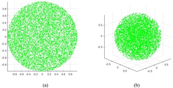
In AHKRA, non-normal and correlated random variables are transformed into independent standard normal first. The adaptive sampling will subsequently take place in standard normal space. Recently, many studies have proposed to use adaptive sampling regions to replace MCS samples as the candidate samples for adaptive Kriging. However, these adaptive sampling regions are based on EGRA or n-sigma rule and thus have unnecessary samples that need to be removed. This problem is alleviated by removing samples with a joint probability density lower than a particular value. The approach is commonly called rejection sampling. However, rejection sampling still leads to a lot of unwanted samples in proportion to the accepted samples. As the dimension of the problem grows, the acceptance ratio becomes excessively small. Figure 2 illustrates an example with a radius of one in a unit hypercube. The acceptance rate (green area) for rejection sampling drops significantly from ~78% to ~53% as the dimension increases from 2 to 3. In a 5-dimensional hypercube, the acceptance rate further drops to merely ~0.2%, which is highly inefficient.
Rejection sampling (a) 2-dimension with ~78% acceptance rate and (b) 3-dimension with ~53% acceptance rate.

Instead of using a truncated sampling region as the candidate pool, AHKRA adopts a hyperball as its domain. By directly sampling in a hyperball, the proposed algorithm can avoid the drawback of using rejection sampling. Sampling uniformly distributed random numbers inside a hyperball can be done by following Muller's algorithm that follows (Muller, Reference Muller1959):
 $${\boldsymbol x} = \displaystyle{{RU^{1/d}} \over {\Vert {{\boldsymbol Z}} \Vert }_2}{\boldsymbol Z},$$
where R is the radius of the hyperball, U is a uniformly distributed random number, Z is a d-dimension standard normal random number, and  $\Vert {\cdot}\Vert_2$ denotes Euclidian norm.
The radius of the hyperball is set to represent the precision of the reliability analysis. The failure region may not be entirely represented by the hyperball with too small of a radius, resulting in an inaccurate estimation of the probability of failure. On the other hand, a larger radius can cover a lower joint probability density, but it may incur unnecessary costs. Thus, a balance between accuracy and computational cost needs to be achieved. So, in AHKRA, the radius is determined by the number of samples needed to calculate a probability of failure with a target coefficient of variation (COV; Echard et al., Reference Echard, Gayton and Lemaire2011). The hyperball's radius is calculated by:
 $$n_{\rm {req}} = \displaystyle{{1-\widehat{{P_{\rm f}}}} \over {{\rm CO}{\rm V}^2\widehat{{P_{\rm f}}}}},$$
 $$R = {-}\Phi ^{{-}1}\left({\displaystyle{1 \over {n_{\rm {req}}}}} \right),$$
where  $\widehat{{P_{\rm f}}}$ is the estimated probability of failure, COV is the target coefficient of variation, which in this paper is determined to be 0.05, and Φ−1( ⋅ ) denotes the inverse distribution function of standard normal distribution.
AHKRA algorithm
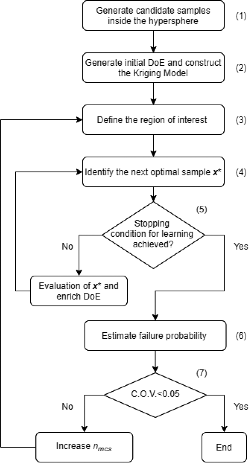
The flowchart of the proposed AHKRA method is illustrated in Figure 3. The AHKRA method is composed of a nested loop: the inner loop deals with the active learning process of finding samples to enrich the Kriging model, while the outer loop deals with adjusting the region of interest that dictates the candidate samples for the model refinement process.
A global flowchart of the proposed AHKRA algorithm.

The entire process of the proposed framework is composed of the following steps:
1. Generate candidate samples inside the hyperball. N 0 samples are generated inside a sufficiently large hyperball domain. Muller's algorithm in Eq. (14) can be used to generate uniformly distributed samples inside the hyperball. In this paper, a radius of six, which is enough to deal with a reasonably low failure probability, P f ≥ 10−9(Φ( − 6)), is deemed enough to cover the area of interest. A larger hyperball may be used depending on the need of the user. The population size N 0 of 104 samples is considered to be a good trade-off between accuracy and computation effort.
2. Generate initial design of experiment (DoE) and construct the Kriging model. The DoE in this study is defined as the group of samples used to train the Kriging model. The initial DoE consists of experimental samples constructed by generating N 1 samples using Latin Hypercube Design (LHD) in the standard normal space. These samples are then evaluated on the original limit state function and used to construct the Kriging model. An ordinary Kriging model with a Gaussian correlation function is chosen.
3. Define the region of interest for the model refinement process. The candidate samples for the model refinement process are chosen according to the radius computed using Eqs (15) and (16). All the candidate samples with a radius higher than the radius determined will be excluded from the candidate pool. It is recommended to use a moderate value for n req in calculating the radius for the first iteration; the value will be adjusted automatically once the estimated probability of failure is calculated. The suggested value for the initial n req is 104.
4. Identify the next optimal sample x* to enrich DoE. The learning function is computed for every sample in the region of interest. The learning function utilized the Kriging prediction
 $( \mu _{\hat{G}})$ and variance ($\sigma _{\hat{G}}$) to determine the next best point to incorporate into the Kriging model. In this study, the ERF function is utilized as the learning function, which is defined as (Yang et al., Reference Yang, Liu, Gao, Zhang and Gao2015):(17)where Φ( ⋅ ) and φ( ⋅ ) denote the cumulative distribution function and the probability density function of standard normal distribution, respectively. The ERF function indicates the risk of a sample being wrongly predicted by a Kriging model. Thus, the sample with the highest ERF value is chosen as the next optimal sample x*.$${\rm ERF}( {\boldsymbol x} ) = {-}{\rm sign}( {\mu_{\hat{G}}} ) \mu _{\hat{G}}\Phi \left({-{\rm sign}( {\mu_{\hat{G}}} ) \displaystyle{{\mu_{\hat{G}}} \over {\sigma_{\hat{G}}}}} \right) + \sigma _{\hat{G}}\varphi \left({\displaystyle{{\mu_{\hat{y}}} \over {\sigma_{\hat{y}}}}} \right),$$
5. Check the learning stopping condition. The model refinement phase is stopped when the learning stopping condition is reached. The stopping condition corresponds to the learning function value of the next optimal sample x*. For the ERF function, the threshold value is defined as ERF(x*) ≤ 1 × 10⁻⁴. If the stopping condition is not satisfied, the optimal sample x* is evaluated and added to DoE. Once added to the DoE, the sample is removed from the candidate pool to avoid duplicated samples. The method then iterates and goes back to Step 4.
6. Estimate the probability of failure. Once the leaning stopping condition is satisfied, the model is deemed accurate enough to represent the area of interest. The probability of failure is estimated using MCS, with the limit state functions replaced by the trained Kriging model. The probability of failure is estimated by the equation below:
(18)where$$\widehat{{P_{\rm f}}} = \displaystyle{{n_{\mu _{\hat{G}} \le 0}} \over {n_{{\rm MCS}}}},$$$n_{\mu _{\hat{G}} \le 0}$ is the number of samples with Kriging prediction $( {\mu_{\hat{G}}} )$ less or equal to zero.7. Check the coefficient of variation stopping condition. Once the estimated probability of failure is estimated, the coefficient of variation is checked to ensure that enough samples are generated to obtain a reliable estimation. Here, a coefficient of variation lower than 0.05 is deemed acceptable (Echard et al., Reference Echard, Gayton and Lemaire2011). The coefficient of variation is calculated by:
(19)If the stopping condition is not satisfied, nMCS is increased, and the method returns to Step 3 to update the area of interest to match the estimated probability of failure.$${\rm CO}{\rm V}_{\widehat{{P_{\rm f}}}} = \sqrt {\displaystyle{{1-\widehat{{P_{\rm f}}}} \over {\widehat{{P_{\rm f}}}\;n_{{\rm MCS}}}}}. $$8. The AHKRA algorithm terminates. The proposed algorithm terminates when the coefficient of variation is lower than 0.05.


Discussion
The proposed AHKRA is an active learning algorithm that uses an adaptive hyperball as its sampling region. Other similar algorithms, such as ISKRA (Wen et al., Reference Wen, Pei, Liu and Yue2016), AKOIS (Zhang et al., Reference Zhang, Wang and Sørensen2020), and AFBAM (Song et al., Reference Song, Zhang, Zhuang, Yu and Song2021), also generate an alternative sampling region to replace the MCS samples. Although these algorithms appeared similar, several key features set the proposed AHKRA apart from the previously stated algorithms. First, AHKRA directly samples in the hyperball. This is more efficient than generating samples in an n-sigma sampling region, especially when the dimension is high. Second, another novel feature of AHKRA is that it represents the precision of the reliability analysis by using the radius of the hyperball rather than using joint probability densities. Third, AHKRA determines the radius according to the number of samples required to calculate the estimated probability of failure with a target coefficient of variation.
Sensitivity analysis of parameters
A sensitivity analysis is conducted to investigate the optimal parameter for AHKRA. The algorithm has three parameters that can be modified: candidate sample size (N 0), initial DoE size (N 1), and the number of required MCS samples (n req). However, the N 0 parameter has a constant value throughout the reliability process. The N 1 should start small since the additional samples will be added by the active learning process, while the n req will be adjusted automatically in Step 3. Therefore, the N 0 parameter has the most significant impact on the reliability result compared with the other parameters. In order to obtain the optimal parameter, the AHKRA will be tested on the following reliability problem with four random variables that follows x 1…4 = N(10,3). The limit state function reads:
 $$G( {\boldsymbol x} ) = x_1^2 + 5x_1 + 2x_2^2 + 7x_2 + x_3^2 -8x_3 + x_4^2 + 5x_4-200.$$
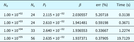
The reliability result of the problem is listed in Table 1. The table shows that as the number of candidate samples grows, so does the Kriging prediction. However, the computing cost of Kriging is low, it is not completely free; hence, as the number of candidate samples grows, the computational cost will become increasingly evident. A larger candidate sample also translates to more information for the Kriging model to account for, which increases the number of DoE required, as seen in Table 1. It is shown that after 104 samples, the improvement in the Kriging model has no significant impact on the probability of failure while needing a substantially larger computing cost. As a result, the population size (N 0) of 104 samples is thought to be a suitable compromise between accuracy and computing effort.
The reliability result of the sensitivity analysis

Note: Ns is the average number of samples in the DoE; Pf is the average probability of failure; β is the reliability index; err is the average relative error calculated in Eq. (22).
Numerical examples
The performance of the proposed AHKRA method is tested on 12 reliability problems with various characteristics. The problems consisted of ten mathematical problems with different dimensions and two engineering practical problems. In each case, the reference probability of failure is estimated using crude Monte Carlo Simulation. The comparison criteria include the total number of samples and relative error. Reliability Index (β) is used when calculating the relative error because it emphasizes a low probability of failure. The reliability index can be calculated by
 $$\beta = {-}\Phi ^{{-}1}( {P_{\rm f}} ), $$
where Φ−1(x) is the standard normal inverse function. The relative error using the reliability index can be calculated by
 $${\rm err} = \displaystyle{{\vert {\hat{\beta }-\beta_{{\rm MCS}}} \vert } \over {\beta _{{\rm MCS}}}} \times 100\%. $$
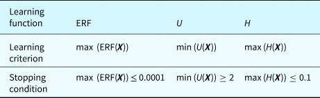
For the practical case, the AHKRA method will be compared with several recent Kriging-based methods: Adaptive Failure Boundary Approximation Method (AFBAM; Song et al., Reference Song, Zhang, Zhuang, Yu and Song2021) and AK-MCS (Echard et al., Reference Echard, Gayton and Lemaire2011) with different learning functions, namely AK-MCS + ERF, AK-MCS + U, and AK-MCS + H. For comparison, all methods start with an initial sampling space of 104 samples and an initial DoE of 15 samples. Since the initial DoE is random, each method is performed ten runs to measure its robustness. The learning criterion and stopping condition for each learning function used in this study are listed in Table 2.
Learning and stopping conditions for each learning function

Mathematical cases
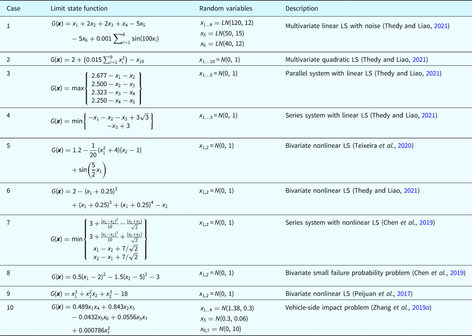
In order to validate the performance of AHKRA, ten different mathematical problems with different dimensions are used. In order to validate the performance of AHKRA, ten different mathematical problems with varying conditions are assessed over ten runs: highly nonlinear limit state function, non-normal distribution, different dimensional problems, and multiple failure modes with series or parallel system. The details of the problems are shown in Table 3.
Mathematical cases

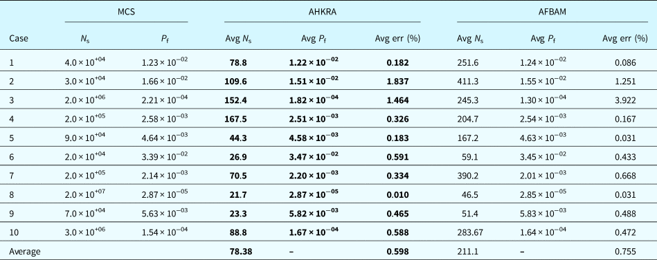
The reliability results of the mathematical cases are shown in Table 4. As can be seen in Table 4, AHKRA can consistently obtain a good approximation over multiple problems with fewer samples (average of 78.38) than AFBAM (average of 211.1). This is because AFBAM's multiple stopping conditions hinder its efficiency. Aside from the efficiency issue, the AFBAM also has a difficulty in solving Case 2. The AFBAM algorithm cannot converge and continue adding non-essential samples until no more samples are left because the screened candidate samples based on the distance to the classification boundary are all used in the DoE. The convergence difficulty is caused by the inefficiency of generating important candidate samples in a high-dimensional problem.
The reliability result of mathematical cases

Note: Avg Ns is the average number of samples in the DoE; Avg Pf is the average probability of failure; Avg err is the average relative error calculated in Eq. (22).
Significance of bold values are to highlight the proposed AHKRA performance.
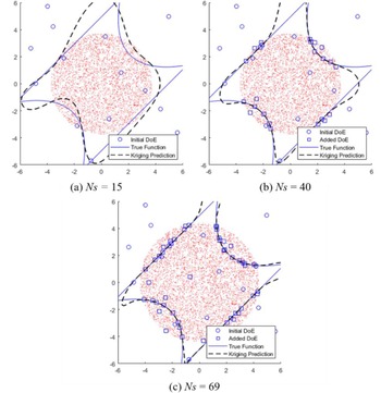
The process of picking and enriching samples in AHKRA is illustrated in Figure 4 where AHKRA is applied to solve the two-dimensional nonlinear problem in standard normal space. AHKRA starts with 15 samples in the initial DoE, as shown in Figure 4a. The Kriging prediction yields a dashed line as the predicted limit state function, whereas the true function is shown as a solid line. AHKRA then finds the most informative samples to add to the DoE, which is shown in Figure 4b. The model will keep improving the prediction until the limit state is well-defined enough. Here, a larger radius is needed for a low probability of failure, so AHKRA determines a suitable radius based on the estimated probability of failure. Observe the increase in radius from Figure 4b, c. By selecting an appropriate radius, the AHKRA algorithm can concentrate on the area with enough impact on the failure probability, thus avoiding unnecessary function evaluation.
Illustration of AHKRA for the series system with the nonlinear limit state.

Practical cases
Dynamic nonlinear oscillator
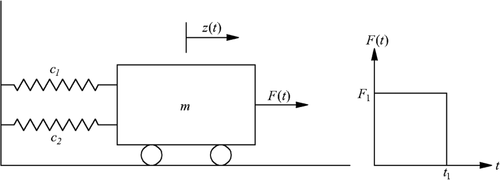
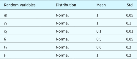
The next case is the dynamic nonlinear oscillator (Pan and Dias, Reference Pan and Dias2017; Kim and Song, Reference Kim and Song2020), shown in Figure 5. The parameters of the random variables are listed in Table 5. The limit state function is formulated as follows:
 $$G( {c_1, \;c_2, \;m, \;r, \;t_1, \;F_1} ) = 3r-\vert {s_{{\rm max}}} \vert ,$$
 $$s_{{\rm max}} = \left\{{\matrix{ {\displaystyle{{2F_1} \over {m\omega_0^2 }}}, \hfill & {t_1 \ge \displaystyle{\pi \over {\omega_0}}}, \hfill \cr {\displaystyle{{2F_1} \over {m\omega_0^2 }}\sin \left({\displaystyle{{\omega_0t_1} \over 2}} \right)}, \hfill & {t_1 < \displaystyle{\pi \over {\omega_0}}}, \hfill } } \right.$$
where  $\omega _0 = \sqrt {{{c_1 + c_2} \over m}}$, s max is the maximum displacement of the oscillator, and r is the yielding displacement of the springs.
Dynamic nonlinear oscillator.

Characteristic of random variables for the dynamic nonlinear oscillator

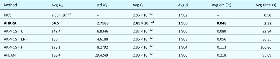
The estimation results are compared in Table 6. The AHKRA method shows excellent efficiency and consistency while attaining high accuracy. All the other methods, except AHKRA, require a large number of samples to perform the estimation, whereas AHKRA only requires an average of 54.5 samples, which is less than half of what is required for the other methods. The faster convergence happens by using LHD to generate the initial DoE, which covers more area than random sampling from the candidate pool. Although AFBAM also uses LHD for the initial DoE, it has multiple stopping conditions aside from the usual learning stopping condition, making it too conservative and less efficient.
Reliability results of the dynamic nonlinear oscillator

Note: std Ns is the average sample standard deviation of the number of samples in the DoE; Avg β is the average reliability index; Avg time is the average computation time.
Significance of bold values are to highlight the proposed AHKRA performance.
Two-bay six-story steel frame structure
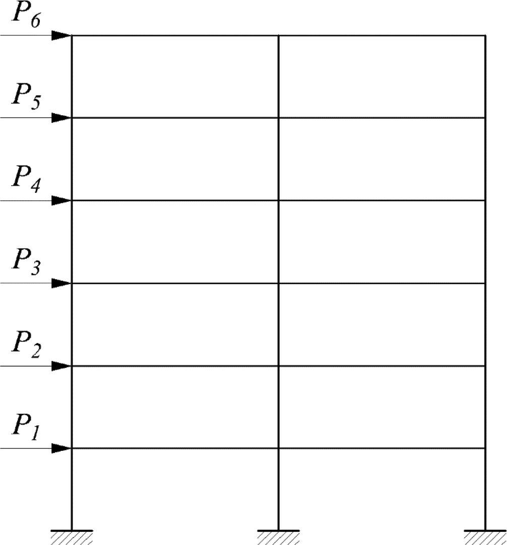
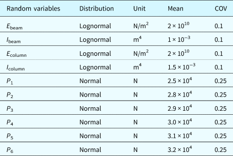
The application of AHKRA is further showcased in a two-bay six-story steel frame structure (Zhang et al., Reference Zhang, Wang and Sørensen2019b). This case is illustrated in Figure 6. Each story in the structure is 3 m in height, and each bay is 7.5 m in width. The structure is subjected to lateral loadings, which are applied in every story. The random variables of the frame structure are as follows: the modulus of elasticity E, the moment of inertia I, and lateral loads P 1–P 6. The details of these random variables are listed in Table 7. The limit state function for the structural reliability analysis is formulated as:
 $$G( {\boldsymbol x} ) = d_0-D_{{\rm max}}( {\boldsymbol x} ), $$
where d 0 is the allowable drift, which is assumed to be 33 mm, and D max(x) is the maximum inter-story drift obtained using a linear finite element model assuming that all members are axially rigid.
Two-bay six-story steel frame structure.

Characteristic of random variables for the two-bay six-story steel structure

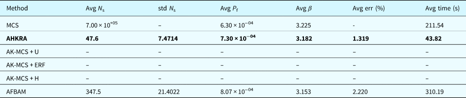
Table 8 compares the proposed AHKRA method with AK-MCS + U, AK-MCS + ERF, AK-MCS + H, and AFBAM. Overall, AHKRA provides a more accurate estimation using fewer samples than the other methods. Facing a small failure probability, the AK-MCS approach encounters difficulties. First, if the initial DoE cannot capture the failure region, even with a large number of samples, the AK-MCS approach cannot yield estimates of the failure probability. Second, as more samples have to be incorporated into the DoE, the Kriging prediction becomes more expensive and often runs out of memory quickly. The AFBAM method, while providing a close estimate, takes 7.3 (347.5/47.6) times more samples than AHKRA. This problem is similar to Case 2 of the mathematical case, in which not enough candidate samples near the limit state function are generated since the majority of the samples are generated outside the crucial area (hyperball).
Reliability results of the two-bay six-story steel structure

Significance of bold values are to highlight the proposed AHKRA performance.
Conclusion
The present study develops an adaptive sampling approach that focuses on a hyperball-based sampling region to estimate the probability of failure in reliability analysis. The proposed AHKRA method picks samples in a hyperball instead of an n-sigma rule-based sampling region. AHKRA uses the radius of the hyperball to express the precision of reliability analysis as an alternative to using joint probability densities. The AHKRA method takes samples from the hyperball, the radius of which is determined by the number of samples needed to calculate a probability of failure with a given coefficient of variation. The radius of the hyperball is iteratively updated to achieve a balance between accuracy and efficiency.
The performance of AHKRA has been tested on ten mathematical cases with various characteristics and two practical cases: a dynamic nonlinear oscillator and a two-bay six-story steel structure. In each case, the AHKRA method consistently yields a more accurate estimate of the failure probability with relatively low computation time compared with other Kriging-based methods. The numerical examples demonstrate the superior performance of AHKRA to previous methods in different circumstances: nonlinear limit state function, non-normal distribution, small failure probability, multiple failure modes, and practical frame structure. The case studies confirm the promising applications of the proposed AHKRA method.
Data availability statement
The data that support the findings of this study are available from the corresponding author upon reasonable request.
Conflict of interest
The authors have no known competing financial interests or personal relationships that could have appeared to influence the work reported in this paper.
I-Tung Yang is Professor in the Civil and Construction Engineering Department at National Taiwan University of Science and Technology. He was seconded as President of Taiwan Construction Research Institute from 2015 to 2018. His areas of expertise include construction management, computational intelligence, decision-making and risk analysis. He received his Ph.D. in Civil Engineering (2002), Master of Industrial Engineering (1999), and Master of Construction Management (1996), all from the University of Michigan, Ann Arbor.
Handy Prayogo is a Ph.D. candidate in the Civil and Construction Engineering Department at National Taiwan University of Science and Technology. His research interests include artificial intelligence, machine learning, reliability analysis, and optimization.