





Highlights
What is already known?
-
• Common effect (CE) and fixed effects (FES) models in meta-analysis estimate the person-average effect size using inverse variance weights, while limiting generalization to those studies included in the analysis. Random effects (RE) models allow for generalization to a broader population, yet the person-average effect size is not always the estimated parameter.
-
• The current practice meta-analytic models all include assumptions on the study effect sizes: they are common across all studies (CE), there are multiple, fixed, effect sizes (FES), or the observed effect sizes are a random sample from a distribution of effect sizes (RE).
What is new?
-
• Estimators that are rooted in sampling theory are presented, that allow for generalization to a defined population while estimating the person-average effect size.
-
• New estimators require assumptions that are different from current practice meta-analytic models that can be verified with covariate and population data.
-
• The person-average and study-average effect sizes can differ due to two correlations: correlation between estimated weights and effect sizes, and correlation due to true weights and effect sizes (which may be due to study design).
Potential impact for RSM readers
-
• Researchers are introduced to new meta-analytic estimators to estimate person-average effects while generalizing to a broader population, as well as guidance on how to decide between possible models.
-
• An emphasis on separating the design and analysis of a meta-analysis is presented to allow researchers to decide a model that aligns with research goals.
1 Introduction
Inverse-variance weights have been part of meta-analysis since its origin (e.g., see Hedges and OlkinReference Hedges and Olkin1) and were originally selected for efficiency, ensuring the meta-analytic average T to have the smallest standard error possible. For example, in the common effect (CE), also known as fixed effect, model, weights are inverse to the sampling variance
$v_i$
 , leading to weights that are proportional to the sample size
$n_i$
 . In comparison, in the random effects (RE) model, the weights are inverse to the unconditional variance,
$v_i+\tau ^2$
 , where
$\tau ^2$
 is the between-study variation. This case, especially when
$\tau ^2$
 is large, leads to closer to equal weights. Importantly, under the assumptions used to derive these weights, any weighted estimator—including CE and RE—produces an unbiased estimate of the true effect
$\theta $
 , so long as it is assumed the weights are fixed.
As a result, the choice between the CE and RE models has largely been framed as a question of generalization: if
$\theta $
 is specific to the studies included (conditional), then a CE model is appropriate, whereas when
$\theta $
 is for a broader population than those included studies (unconditional), then RE is appropriate. Tied to the CE model is the CE assumption, an assumption that “all studies in the meta-analysis share a common (true) effect size.”Reference Borenstein, Hedges and Higgins2 As this assumption is tied to only those studies observed in the analysis, conclusions gained from the effect size estimate can only be applied to those observed studies. One may argue that conclusions can extend to any “similar” studies (i.e., ones where the CE assumption would apply had they been observed), but there is no way to determine a population of these studies beforehand (see Hedges and VeveaReference Hedges and Vevea3 and Hunter and SchmidtReference Hunter and Schmidt4). The RE model, on the other hand, considers the observed studies to be a random sample of a larger population of studies. Rather than estimating the true CE, the RE model attempts to estimate the mean of a distribution of true effect sizes. Since the results of meta-analyses are clearly intended for use beyond the studies included, this suggests that RE models should nearly always be appropriate. For example, in medicine, meta-analytic results are provided in the Cochrane Library, intended for physicians to turn to when choosing treatments for their patients; similarly, in education research, results are provided in the What Works Clearinghouse (WWC), intended for school leaders and decision-makers to turn to when selecting curricula for their schools.
The question of generalization in meta-analysis is not just whether results can be generalized, but how and to whom they are generalized. If we accept that the RE model allows for unconditional inference to a population—what does this population look like? Moreover, are we generalizing to other studies or individuals? Consider a population of 100 people, divided into two studies. In Study 1, we have a sample of 90 of these people, where the true effect size for these 90 people is 1. In Study 2, we have a sample of the other 10 people, where their true effect size is 0. Therefore, the true average individual effect size in our population is 0.9. Moreover, assume each study estimated their respective effect sizes accurately, with variance inversely proportional to each sample size. Then, a CE model would lead to an effect size estimate of 0.9, while an RE model would lead to an effect size estimate of 0.5. This example illustrates the fallacy of applying group-level findings to individuals. The RE model, while providing unconditional inference, may estimate the study-level average rather than person-level average, especially in cases of high heterogeneity.
Therefore, meta-analytic issues with generalization do not only concern the question of if we can generalize, but also of how to generalize conclusions to individuals. In this article, we thus ask: What if the goal of the meta-analysis is to provide an estimate of the person-average effect (like CE) for a population of people broader than those included in the studies sampled (like RE)? To our knowledge, no current meta-analysis model exists to handle this situation—in which effects vary and unconditional inferences are desired for individuals, not studies. To do so, we re-frame meta-analytic models in terms of person-specific effects (instead of study-specific effects) and examine different possible sampling processes that could lead to the data observed in a study and meta-analysis.
In this article, we focus on small meta-analyses for a clearly defined intervention, where we consider only the standardized mean difference (SMD) as the effect size. These types of meta-analyses are common in research clearinghouses—for example, the WWC in education. In Section 2 of this article, we begin by providing an overview of current meta-analytic models. In Section 3, we highlight the fallacy of applying group-level findings to individuals in the context of meta-analysis, as well as explore conditions under which differences between the two arise. Building off of Shuster,Reference Shuster5 we show that these differences occur when both the weights and the effect sizes can be conceived of as random variables. When these are correlated, the exchangeability assumption in the RE model is violated. By examining the weights used in both the CE and RE models, we show that there are two separate types of correlation that can occur here—one of which is an artifact correlation often discussed in the selection bias literature,Reference Rothstein6 while the other is a correlation induced by the relationship between true weights and effect sizes. The latter has received less attention in the meta-analytic methods literature, though it has been discussed in applications.
In Section 4, we focus on person-specific effects and introduce new meta-analytic models based off standard sampling frameworks—namely, simple random sampling (SRS), stratified SRS, and cluster sampling—and argue that in general, the cluster sampling framework is most appropriate given how recruitment occurs in most studies. These frameworks start with the conceptualization of a defined, finite population of individuals for which inference is desired (e.g., high school students in California, diabetes patients in the United States, etc.). We show how weights under these models could be derived and compare and contrast these resulting estimators with those of current meta-analytic methods. Section 5 discusses the usefulness of these models and how to use them in practice, followed by Section 6 where we illustrate this choice of weights in a few different meta-analytic examples. These examples are focused on small meta-analyses of clearly defined interventions and on the SMD effect size. Holding the intervention fixed allows us to examine other sources of variation in effects—for example, based upon persons and settings. We conclude with a discussion of limitations and further directions for this research in Section 7.
2 Current practice
In this section, we begin by briefly reviewing three common meta-analytic estimators and weights. In general, meta-analytic models begin by relating the estimated effect size
$T_i$
 to the true effect size
$\theta _i$
 in study
$i = 1,\ldots ,k$
 via the model:

Here, the
$T_i$
 are assumed to be unbiased estimates of the parameters
$\theta _i$
 with known sampling variance
$v_i$
 . For example,
$\theta _i$
 could be the SMD
$\delta _i$
 , estimated by Hedges g.
There are three common meta-analytic models, and each of these conceptualize and model
$\theta _i$
 differently. In the CE model, it is assumed that
$\theta _i = \theta $
 for all studies; typically, in this framework, the studies are considered “fixed” and inferences are conditional only on the studies included in the meta-analysis, all of which are assumed to be estimating the same parameter. In the RE model, the
$\theta _i = \theta + \eta _i$
 are assumed to be random draws from a larger population of studies, where
$\theta $
 is the average effect,
$\eta _i \sim N(0,\tau ^2)$
 , and
$\tau ^2$
 is the degree of variation in effects. The RE model thus provides unconditional inferences, enabling clear generalizations beyond the sample of studies in the meta-analysis. Finally, the fixed effects (FES) model offers a middle ground by assuming that the
$\theta _i = \theta + \eta _i$
 differ, like the RE model, while treating the studies as “fixed,” thus focusing on conditional inferences to the included studies, like the CE model.
The simplest goal in a meta-analysis is to estimate the parameter
$\theta $
 , and a measure of its precision, such as its variance or a confidence interval. In general, each of these models provides an estimator of
$\theta $
 of the form:

Typically, inverse variance weights are used, where the form of the variance depends upon the model (CE, RE, and FES) selected. More specifically, in the CE model,
$w_i = \frac {1}{v_i}$
 is used, whereas in the RE model,
$w_i = \frac {1}{v_i + \tau ^2}$
 is used; in the FES model, different weights have been proposed, with some suggesting CE weights and others equal weights,
$w_i = \frac {1}{k}$
 (e.g., see Bonett,Reference Bonett7 Rice et al.,Reference Rice, Higgins and Lumley8 and Laird and MostellerReference Laird and Mosteller9). Under the assumption that the weights are fixed (known), it is easy to show that for any set of weights T is an unbiased estimator of
$\theta $
 , so long as
$E[\theta _i] = \theta $
 . This condition also holds if the weights are considered random, and it is assumed that
$Cov(w_i,T_i) = 0$
 ; this is referred to as an exchangeability assumption in the RE model.Reference Shuster5
If the weights are indeed inverse variance, the resulting model-based sampling variance estimator can be written

Alternatively, for any general weights, the sampling variance can be estimated using robust variance estimation (RVE),Reference Hedges, Tipton and Johnson10 resulting in the estimator,

where
$A_i$
 is an adjustment value that is intended to improve coverage and reduce errors in small samples. For the general RVE estimator, TiptonReference Tipton11 investigates three possible adjustments—HC1, HC2, and HC3—and shows that the HC2 adjustment generally contains Type I error appropriately when there are at least four studies. Zejnullahi and HedgesReference Zejnullahi and Hedges12 further investigate these adjustments in smaller samples (including just two studies) and when the focus is on the average estimator T. They show that, in this case, the HC2 estimator results in the adjustment
$A_i = \left (1-w_i/\sum _{i=1}^k w_i\right )^{-1}$
 and also verify that this works well with four or more studies. When fewer studies are included, they show that the HC3 adjustment,
$A_i = \left (1-w_i/\sum _{i=1}^k w_i\right )^{-2} $
 , performs better. Table 1 shows a summary of the current practice models.
Current practice meta-analytic models

Table A1 Long description
The table consists of five columns: Parameter, C E, F E S (Unweighted), F E S (Weighted), and R E.
* Parameter row: C E is Common theta. F E S (Unweighted) is theta equals 1 over k times the summation from i equals 1 to k of theta sub i. F E S (Weighted) is theta equals the numerator summation from i equals 1 to k of 1 over v sub i times theta sub i all over the denominator summation from i equals 1 to k of 1 over v sub i. R E is theta equals E of theta sub i.
* Weights row: C E is 1 over v sub i. F E S (Unweighted) lists Multiple options. F E S (Weighted) is 1 over v sub i. R E is 1 over the quantity v sub i plus tau-squared hat.
* Variance row: C E, F E S (Weighted), and R E all share the formula 1 over the summation from i equals 1 to k of w sub i. F E S (Unweighted) is Weight dependent.
* Generalization row: C E, F E S (Unweighted), and F E S (Weighted) are Conditional. R E is Unconditional.
* Assumptions row: C E is for all i, theta sub i equals theta. F E S (Unweighted) and F E S (Weighted) list None. R E shows w sub i models theta sub i.
2.1 Choosing between models
Much has been written about the choice of meta-analytic model, particularly the choice between the CE and RE models (see Borenstein et al.,Reference Borenstein, Hedges and Higgins2 Hedges and Vevea,Reference Hedges and Vevea3 and Erez et al.Reference Erez, Bloom and Wells13). Theoretically, these choices boil down to answering two questions: (1) Could average-effects vary across studies? (2) Should the studies be considered fixed or random?
2.1.1 Could average-effects vary across studies?
A first consideration for selecting the appropriate model has to do with the degree of variation expected in the true study-specific effect sizes
$\theta _i$
 . If they are expected to vary, then an FES or RE model is more appropriate, whereas if they can be assumed to not vary, a CE model is appropriate. Importantly, Hedges and PigottReference Hedges and Pigott14 note that the choice of model due to observed heterogeneity should not be based upon a formal statistical test, since this test (particularly with
$k<10$
 ) is under-powered. For a specific intervention, in the CE model,
$\theta ^{CE}$
 is the treatment effect for all individuals. Yet, this treatment effect applies only to those studies (and thus people) included in the meta-analysis, with no extrapolation to a defined population.
2.1.2 Should studies be considered fixed or random?
If it cannot be assumed that effects are the same across studies, the next consideration is if the studies included in the meta-analysis should be considered as “fixed” or “random.”
Fixed effects. In the FES model, the studies are considered “fixed,” and the inferences are considered conditional on the studies included in the meta-analysis. In practice, however, this is a restrictive assumption, since a primary goal of substantive research is to discover conclusions that can be generalized beyond the samples included in studies.Reference Hunter and Schmidt4, Reference Overton15
In the FES model, it is not obvious how to weight the studies, since each effect size is assumed to differ. One approach is to weight the studies equally,
$w_i = \frac {1}{k}$
 , whereas another instead uses the same inverse-variance weights as in the CE model,
$w_i = \frac {1}{v_i}$
 . Importantly, the average effect size parameter
$\theta ^{FES}$
 thus depends upon the choice of weights, and much of the literature has focused on how to make this decision (see Bender et al.,Reference Bender, Friede and Koch16 Bonett,Reference Bonett7 Laird and Mosteller,Reference Laird and Mosteller9 and Rice et al.Reference Rice, Higgins and Lumley8).
Random effects. In the RE model, the included studies are considered to be a random sample of a larger population of studies. This distinction between the sample and population can be conceptually difficult in a meta-analysis, especially given the focus on a thorough review. HedgesReference Hedges17 noted in introducing the RE model that
One explanation for the elusiveness of these relations derives from a proposal by Cronbach.Reference Cronbach18 He suggests that evaluation studies should consider a model in which each treatment site (or study) is a sample realization from a universe of related treatments. Thus, when evaluators look at “replications” of a treatment across sites, they observe many different treatments, each sampled from some universe of possible treatments.
This suggests that in its original conception, the RE model was an extension to the RE ANOVA model, with the RE representing variation in versions of a treatment, therefore originally considering the treatments as random yet study samples as random samples from the same population. Later conceptualizations have added to this additional sources of variation, for example, different groups of participants, or different designs, dosages, and interventions.Reference Borenstein, Hedges and Higgins2
A question in the RE model is how to characterize the “population.” Hedges and VeveaReference Hedges and Vevea3 have argued that in RE, the population from which the studies (or effect sizes) are sampled can be defined in terms of the observed study characteristics. Laird and MostellerReference Laird and Mosteller9 offer a similar conceptualization, noting that “each study corresponds to a population selected from the universe of populations (many of which have not been conceived, let alone carried out).” Importantly, in both conceptualizations, the population is defined in relation to the studies that have been sampled, not the reverse. Alternatively, Erez et al.Reference Erez, Bloom and Wells13 suggest getting around this by using the RE model to generalize to a hypothetical population of studies rather than a concretely defined one.
Note that in the RE model,
$\theta ^{RE}$
 is the mean of a distribution of true effects in the population:

where K represents all studies in the defined population. These
$\theta _i$
 represent single studies or effect sizes, and therefore we can see that
$\theta ^{RE}$
 is an average of study-specific effect sizes.
Finally, note that the use of the RE model is often limited by technical requirements of the model. In particular, estimation of
$\tau ^2$
 , the between-study variation, requires a minimum of around 8–10 studies.Reference Langan, Higgins and Jackson19 Thus, when an unconditional inference via RE is not possible, analysts may instead turn to the conditional FES model, keeping in mind the limitations on generalization.
3 Individual versus study average effect
In the previous section, we reviewed the standard literature and approach to model selection in meta-analysis. But sometimes the decision between these models is not obvious. For example, what if it is reasonable to expect that effect sizes vary across studies (ruling out CE), but the goal is to estimate the average effect size for individuals, not studies (ruling out RE), in a broader population (ruling out FES)? This goal of developing an approach to estimate a generalizable, person-average effect size is the focus of this article.
In this section, we examine more carefully properties of the estimators of the person-average effect (CE and FES) and compare these to properties of the estimator of the study-average effect (RE) in order to understand when they are the same and when they differ. To do so, we focus on estimators of the form:

where
$w_i^*$
 is an estimate of a true weight
$\pi _i$
 (where here both are relative weights, i.e.,
$\sum w_i^*= \sum \pi _i =1$
 ), and
$T_i$
 is an unbiased estimate of a study average effect size
$\theta _i$
 . Throughout this section, we further assume that the true sampling variance is
$V(T_i) = V_i$
 , which is estimated by
$v_i$
 , that the true study average effects have
$E(\theta _i) = \theta $
 and
$V(\theta _i) = \tau ^2_\theta $
 . Notice that
$\theta $
 is thus an unweighted average of the study-specific
$\theta _i$
 values.
Here, we compare properties of two estimators. The first is the CE/FES estimator,
$T^{CE}$
 , where
$w_i^* = w_i^{CE*}= 1/v_i$
 , and where these weights estimate
$\pi ^{CE}_i = 1/V_i$
 , where
$V_i$
 is known. Note that we use CE in the superscript here, but the weights are the same as those used in the FES model. The second is the RE estimator,
$T^{RE}$
 , where
$w_i^* = w_i^{RE*}= 1/(v_i + \hat {\tau }^2_\theta )$
 ; these weights estimate
$\pi ^{RE}_i = 1/(V_i + \tau ^2_\theta )$
 which are also known.
3.1 When all studies are observed (conditional)
When the sample S of k studies in the meta-analysis represent all of the studies in the population, or when results are conditioned on these studies, the expected values of
$T^{CE}$
 and
$T^{RE}$
 are as follows:


where
$\theta ^{CE}_k$
 and
$\theta ^{RE}_k$
 are defined as

The proofs of these equations can be found in the Appendix. Notice that since
$w_i^{CE*} \propto n_i$
 , the CE parameter
$\theta _k^{CE}$
 is often interpreted as the person-average effect size for those individuals included in the meta-analysis, since studies are weighted proportional to their sample sizes.
Here too, for a general A,

and
$\rho _{wt} = corr(w^*_i, T_i)$
 is a correlation between the estimates of some weights and the estimates of the effect sizes. For example, Pustejovsky and RodgersReference Pustejovsky and Rodgers20 show that when using CE/FES weights, when the SMD effect size d is large, correlation between d and inverse variance weights is nonzero. This correlation is also nonzero, though smaller, when using RE weights, particularly when
$\hat {\tau }^2_\theta $
 is large (producing weights that are less variable). Similarly, this correlation may be nonzero as a result of publication bias; for example, PET-PEESE methods look for a relationship between CE weights and the effect size estimates
$T_i$
 .Reference Stanley and Doucouliagos21 Moreover, other methods have been suggested in order to remove this correlation.Reference Nakagawa, Lagisz and Jennions22,
Reference Spake, Mori and Beckmann23
To conclude, when conditioning on the k studies in the meta-analysis, the CE/FES and RE estimators are thus only estimating the same parameter when (a)
$\theta _i = \theta \, \forall i$
 (the CE assumption holds) and (b)
$\rho _{w_{R}t} = \rho _{w_{CE}t} = 0$
 .
3.2 When a random sample of studies is observed (unconditional)
We now consider the case when the k studies in the sample S are instead conceived of as a random sample from K studies in the population, that is, then
$\theta _k$
 itself is a random variable. Now the expected values of
$T^{CE}$
 and
$T^{RE}$
 are as follows:


Again, the proofs of these equations can be found in the Appendix. These equations reveal a few insights, though they might not be immediately obvious. First, if the goal is indeed to estimate the (unweighted) study-average effect size
$\theta $
 , neither the CE/FES or RE estimators are guaranteed to do so without further assumptions. Again, like in the conditional inference case, since
$E(A)> 0$
 , there can be no estimation-induced correlation (
$\rho _{wt}=0$
 ). Additionally, since weights typically vary (
$\tau _\pi> 0$
 ), then (a) either there needs to be no variation in effect sizes (
$\tau _\theta =0$
 ) or (b) an exchangeability assumption must hold (
$\rho _{\pi \theta } = 0$
 ).
When this correlation
$\rho _{\pi \theta }$
 is nonzero, then there is a relationship between the true weights and true effect sizes, akin to an exchangeability assumption in the RE model. Importantly, in standard texts, this exchangeability assumption is a requirement for the development of properties of the RE estimator, though it is rare for meta-analysts to check the validity of this assumption in their analyses. One way this correlation can arise is if the designs of primary studies are based upon power analyses,24 where the sample size (and thus the true weights) are related to the magnitude of the true effect size. Importantly, the problem that is produced when this assumption fails—of estimands depending upon weights—is not specific to meta-analysis. For example, in cluster-randomized trials, Kahan et al.Reference Kahan, Li and Copas25 discuss the conditions under which the person- and cluster-average effect can differ. When they differ, this is referred to as “informative cluster size,” which occurs when there is a relationship between the size of treatment effects and of cluster sizes.
Second, if the goal is to estimate the person-average effect size—which the CE models estimates (since it weights the studies proportional to their sample sizes)—then it can be shown that the RE estimator is biased where

Notice that, again, assuming there is variation in effect sizes and weights across studies (i.e.,
$\tau _\theta>0, \tau _\pi >0$
 ), then this bias is only zero when (a)
$\rho _{\pi _{CE}\theta }\tau _{\pi _{CE}}=\rho _{\pi _{RE}\theta }\tau _{\pi _{RE}}$
 and (b)
$\rho _{w_{CE}t}E(A_{CE}) = \rho _{w_{RE}t}E(A_{RE})$
 . One way for this to be true, of course, is for
$\rho _{\pi _{CE}\theta }=\rho _{\pi _{RE}\theta }=\rho _{w_{CE}t}=\rho _{w_{RE}t}=0$
 , that is, for the exchangeability and estimation-error assumptions to both be met. But importantly, when either (or both) of these assumptions fails, the RE estimator does not provide a means to estimate a generalizable, person-average effect size for the population (which is the goal of this article).
4 A population-based perspective
Often in meta-analysis, the desire is to be able to interpret the estimated effects in terms of a population of individuals—for example, patients, students, etc. As shown in the previous sections, the three available models in meta-analysis—CE, FES, and RE—are either based upon models of studies, not individuals, or do not generalize to a population of individuals. In this section, we begin by reconceptualizing meta-analysis from an individual unit perspective. We show that this is more consistent with how primary study results are parameterized and interpreted.
Instead of starting with the data in hand, we begin with considering a population P of individuals and then examining the possible processes through which samples (studies) could be generated. To do so, we conceive of three different types of samples: simple random samples (SRSs), stratified SRSs (SSRSs), and cluster samples (CSs), notably showing that SRS and SSRS are special cases of CS. We also note that a meta-analysis may not fit perfectly into any of these setups outside of ideal conditions, yet they provide a good framework for theoretical discussion.
The three sampling procedures all have inference goals related to all individuals in the conceived population. Figure 1 shows a generic makeup of
$j=1,\ldots , N$
 different individuals in a finite population P, each with individual treatment effect
$\theta _{Pj}$
 . Note that
$\theta _{Pj}$
 itself cannot be observed. Our parameter of focus is now

This differs from both the CE and RE parameters—it is an individual level parameter, but it is also on the population level. Also, this parameter has an explicit construction, removing any ambiguity about what exactly is being estimated in a meta-analysis. Within the population, any use of stratification or clustering is considered part of the design, but does not affect the parameter. In each case, we discuss how we might conceive of a meta-analysis being sampled in this framework, as well as provide the resulting estimators. Throughout, we focus on the resulting weights that arise under each model, where the shift from model-based estimators (as seen in CE, FES, and RE) to a design-based framework will impact the choice of weights that are used, with weights that are dependent upon the design rather than chosen for efficiency purposes.
Finite population of individuals.
Note: Each icon/color combination represents different types of people in our population, with different sets of observable characteristics related to outcomes.

The goal is to estimate
$\theta $
 from a series of
$i = 1,\ldots ,k$
 samples (studies). We will refer to these interchangeably as samples and studies throughout. In this framework, each sample comes from a population cluster, where the combination of all clusters makes up the entire finite population. Each sample i provides an unbiased estimate
$T_i$
 with variance
$v_i$
 of a cluster average effect size
$\theta _i$
 where

where
$N_i$
 is the population size of cluster i, and
$\theta _{ij}$
 is the individual effect size for individual j in cluster i. Notice now that how these
$\theta _i$
 relate to
$\theta $
 will depend upon how the samples included in the studies are gathered. For simplicity, we will assume that the samples are selected with replacement (or equivalently, that the population
$N_i$
 is much larger than the study sample sizes
$n_i$
 ).
4.1 Cluster sampling
We begin with a cluster sampling framework, as the other sampling methods will then be shown to be special cases of this framework. Here, assume that P is partitioned into
$i = 1,\ldots ,K$
 non-overlapping, independent clusters, each of size
$N_i$
 , where
$N = \sum _{i=1}^K N_i$
 , as seen in the top of Figure 2. In typical cluster sampling, the clusters are intact groups—for example, hospitals and schools—leading to groups of individuals that are more similar to one another than a random sample from the full population would be, although it is not a requirement that the clusters are intact groups. Within each cluster, the average effect size is
$\theta _i$
 , and thus the average effect size in P is related via

Cluster sampling.
Note: Each icon/color combination represents different types of people in our population, with different sets of observable characteristics related to outcomes.

Figure 2 Long description
The diagram consists of two vertical panels.
Top Panel: A population is divided into a grid of six rectangular clusters. The top row contains clusters labeled theta sub 1, theta sub 2, and theta sub 3. The bottom row contains theta sub 4, theta sub 5, and theta sub k. Each cluster contains a heterogeneous mix of blue circles, red plus signs, and green triangles representing different types of people.
Bottom Panel: The same grid is shown, but three specific clusters are selected for sampling. The selected clusters, theta sub 2, theta sub 4, and theta sub k, are highlighted with red borders. Inside each of these three red-bordered clusters, a black circle encompasses a subset of the icons. Arrows point from the center of these black circles to external labels: T sub 2 for the top-middle cluster, T sub 4 for the bottom-left cluster, and T sub k for the bottom-right cluster. The non-selected clusters, theta sub 1, theta sub 3, and theta sub 5, remain with black borders and no internal circles.
In cluster sampling, the sampling proceeds in two stages. First, an SRS of k of K clusters is selected, and then, an SRS of
$n_i$
 individuals is drawn within each cluster. Note that the
$n_i$
 individuals are those that participate in a study which is a part of a cluster, and that a cluster’s
$N_i$
 value is not equal to a study’s
$n_i$
 . The bottom of Figure 2 illustrates this, where the red boxes are the clusters selected in the first stage, and then all units contained in the circles are selected into the samples. Here, we make the assumption that samples within clusters are exchangeable, but the clusters themselves are not.
In this framework, each study will represent a specific cluster of P, and thus there may be varying, true average effect sizes across these clusters, depending on the true mechanism defining the clustering. That is, each cluster has a true average effect size defined in Equation (5). We assume that as a result of the second stage SRS, the estimated average effect size from study i,
$T_i$
 , is an unbiased estimate of
$\theta _i$
 . Thus,
$\theta $
 can be estimated using

where the sum is over all i clusters observed in our sample of clusters (S). The weights used are

This version of T is referred to as the “ratio estimator,” as the denominator includes only the total number of individuals included across the k studies, rather than included in the full population.Reference Lohr26 While this estimator is not unbiased, an unbiased estimator for the cluster sampling framework does exist (see the Appendix). This unbiased estimator, however, requires knowledge of the number and sizes of all clusters in the population, which is likely infeasible under the conceptualization of “potential study” clusters in meta-analysis. The choice of weights as seen in Equation (6) comes directly from estimating population averages in sampling theory. The design-based variance of this estimator requires the number of clusters in the population, K, to be known.Reference Lohr26 By defining clusters abstractly as possible study clusters, this value of K cannot be known (or does not entirely exist). Instead, the sampling variance can be estimated using RVE. As discussed previously, RVE results hold for any set of weights, so the use of
$N_i$
 as weights is valid in variance estimation through RVE.
There are a few comments to make about this framework. First, notice that P is divided into clusters of individuals, where some of these clusters of people may participate in studies. In the meta-analytic case, this means that even if we have correctly identified every study that has been completed, there may still remain “potential studies” in parts of the population that have not been studied. In essence, we are defining our clusters as portions of the population where studies may take place. This abstract approach is more flexible and doesn’t require statements such as “a population of studies,” and rather assumes that there are clusters of individuals that could make up a study.
Second, we have so far assumed that clusters have equal selection probability of
$\frac {k}{K}$
 . Similar to Dahabreh et al.,Reference Dahabreh, Robertson and Petito27 this work considers the role of sampling in meta-analysis, but with a focus on a finite population that extends to cluster sampling, rather than the role of unequal selection probabilities within a superpopulation approach. Our framework can, of course, be generalized to account for unequal probabilities. Because of these different selection probabilities, it may be of use to relax this assumption and consider two-stage cluster sampling estimators that do not require this equal selection probability. To do this, we must define
$\pi _i$
 as the probability that cluster i will be selected into the sample. Note that we will still assume that within each selected cluster, we have a random sample of individuals. Using these unequal selection probabilities, we can apply the Horwitz–Thompson estimator,Reference Lohr26 which results in our estimator T but with weights

where
$\pi _i$
 is the probability that cluster i is randomly sampled. Further development of this approach, however, is beyond the scope of this article.
4.2 Stratified sampling
The stratified sampling case is a special case of cluster sampling where all clusters (interchangeably referred to as strata now) are observed. That is, while in CS we first sample clusters, then individuals within clusters, here we sample individuals from all
$k=K$
 clusters. Figure 3 illustrates this. Like clusters, the strata in this case could be created to be very different or more similar to one another. While in sampling theory these are typically defined in relation to one or two variables, this is not required.
Stratified simple random sample.
Note: Each icon/color combination represents different types of people in our population, with different sets of observable characteristics related to outcomes.

Figure 3 Long description
The diagram consists of two vertically stacked panels, each containing a large rectangle divided into three vertical sections or strata.
Top Panel: Population Distribution
* The left section is labeled theta sub 1 and contains green circles and red triangles.
* The middle section is labeled theta sub 2 and contains green circles, red triangles, and blue plus signs.
* The right section is labeled theta sub k and contains red triangles and blue plus signs.
* Ellipses between the second and third sections indicate additional strata.
Bottom Panel: Sampling Process
* The same three sections are shown with identical icon distributions.
* In the theta sub 1 section, a black oval encircles a group of icons, with an arrow pointing left to a label T sub 1.
* In the theta sub 2 section, a black oval encircles a group of icons, with an arrow pointing up and right to a label T sub 2.
* In the theta sub k section, a black oval encircles a group of icons, with an arrow pointing right to a label T sub k.
* These ovals and T labels represent the selection of a simple random sample from within each distinct stratum.
We assume that P is partitioned into
$i = 1,\ldots , k$
 non-overlapping, independent strata, each of size
$N_i$
 , where
$N = \sum _{i=1}^k N_i$
 . Within each stratum, the average effect size is
$\theta _i$
 , and thus the average effect size in P is related via

Notice that this is exactly the same relationship found in cluster sampling (except here we use k as
$k=K$
 ).
Within each stratum, assume that a sample of
$n_i$
 individuals is drawn from the stratum population of
$N_i$
 individuals via an SRS. Thus, the stratum-specific effect size estimate
$T_i$
 provides an unbiased estimate of
$\theta _i$
 . As a result, the general weighted estimator T will use weights identical to that of cluster sampling:

where the full estimator is

The weights are chosen as in Equation (7) as they are the only weights (or any weights proportional to these) that lead to an unbiased estimator of
$\theta $
 under this design (see the proof in the Appendix). This assumes that the true effect sizes vary, meaning the
$\theta _i$
 are not all equal. The difference between the SSRS and CS frameworks is shown in the variance. As a sample from every stratum is obtained, there is no concern for between-strata variation, and thus the variance of the estimator can be estimated by

There are a few important caveats to this design. First, at least one study from each of the k strata needs to be observed (if multiple studies are provided from the same stratum, these can first be aggregated using the SRS method presented in the next section to obtain the stratum average). For example, it could be that there are 12 strata, but studies are observed from only 10; this is referred to as undercoverage in the sampling literature. In this case, our inference would change and we would no longer be estimating the average effect for all individuals in the population P. Instead, we would need to redefine P to only include those strata that we have, that is, condition on our studies (strata) we observe.
Second, because of stratification, the strata (and resulting SRS samples) should differ from one another with regard to one or more characteristics. For example, this might mean that the average age differs across strata. Sampling theory tells us that the ideal strata are maximally different from one another with regard to covariates that explain variation in the outcome (here stratum specific effect sizes
$\theta _i$
 ). However, while this is optimal for variance reduction, it is not required. Thus, clearly strata will differ, but they may differ in more minimal ways. That is, instead of all individual ages 5–11 in one stratum and those ages 12–18 in another, it could be that both contain individuals with ages 5–18, but those in one stratum are younger, on average, than those in the other. The only requirement here is that the k strata, taken together, fully cover the population P.
4.3 Simple random sample
The final special case of cluster sampling is SRS. Here, we can imagine that the cluster assignments are assigned randomly—leading to no true clustering at all. Thus, any random sample within a randomly assigned cluster will also be a random sample from the entire population, as illustrated in Figure 4.
Simple random sample.
Note: Each icon/color combination represents different types of people in our population, with different sets of observable characteristics related to outcomes.

Assume that each of k studies includes an independent, SRS of individuals in P. This means that the k studies will have samples that are similar to one another on both measured and unmeasured characteristics—for example, average age of participants, average baseline health, and so on. This situation may arise in replication studies, where the population of participants, intervention, and other study characteristics are attempted to be held constant. Because they are SRSs, each study average effect size estimator,
$T_1, \ldots T_k$
 , alone provides an unbiased estimate of
$\theta $
 .
Thus, since every estimate is unbiased and there is no inherent grouping of individuals, any weighted combination of these estimates is unbiased, so long as the weights are not related to the effect sizes. There is a parallel here to the CE model, where any choice of weights (that sum to 1) will lead to an unbiased estimate, so the weights can be chosen to minimize the variance of T, leading to inverse-variance weights

that produce the most efficient estimate of
$\theta $
 . Notice that this means that
$w_i^{SRS} \approx n_i$
 . Note that the full estimator has the same form as both
$T^{CS}$
 and
$T^{SSRS}$
 :

Finally, the resulting variance is the same as that found in CE

5 Why and how to use these models?
By considering meta-analysis from a sampling lens, a few questions arise. First, how do these models differ from current practice models? Second, how should researchers use and decide between these models? As previously mentioned, under current practices, there is no suitable model that allows for generalization to a population while also focusing on an individual, not study, average effect size.
The sampling estimators proposed here offer an alternative to both CE and RE models by considering how study samples are drawn. In standard sampling theory, we take a sample of units from a population, calculate the average for that sample, and generalize the inference to the population. The same logic applies here, while taking into account more complex possible designs (i.e., SSRS or CS). Second, the parameter
$\theta $
 that these sampling models estimate is constructed based on the consideration of a finite population of individuals. In other words, the parameter
$\theta $
 as used in Section 4 has an explicit functional form and is constructed as an average effect size for all individuals in the defined population. Therefore, by starting with a population and the data-generating process, the sampling estimators meet both goals that current meta-analytic models do not.
As with all models, the sampling frameworks proposed here require assumptions about the design and sampling schemes of studies and samples. In practice, it may not be entirely true that the observed studies are a random sample of a population of studies. That being said, current practice meta-analysis models (such as the RE model) also hinge on this assumption. Moreover, while samples within studies may be convenience samples rather than random samples, this feature would have implications on both the proposed models as well as current practice models. By being explicit about the required assumptions, analysts can use the feasibility of these assumptions as well as the guidelines presented next to thoughtfully decide the correct model within the context of their design, data, and research aims.
5.1 How to decide the correct model?
When deciding on which sampling framework fits a particular analysis, there are a few questions that can be considered:
1. What is the population these studies (or individuals) were sampled from? First, the definition of the population P needs to be decided. This can be based on research goals in general, clearly defined inclusion/exclusion criteria, or on the characteristics (location, covariates, etc.) of the observed studies.
2. Is there clustering or grouping in the way study samples were drawn? This can be assessed qualitatively—for example, checking if studies are conducted in different locations, on different age groups, etc. Alternatively, aggregate data from the studies can be used to evaluate if there is grouping or if the samples are each an SRS of the same population P. When the assumption that each sample is an SRS of P holds, then on average, the covariate distributions in the studies should be the same—that is, for a general vector of covariates
$E(\textbf {x}_i|i=1) = E(\textbf {x}_i|i=2) = \cdots = E(\textbf {x}_i|i=k)$
 . This can be examined on the observed data in a meta-analysis using a
$\chi ^2$
 test or ANOVA. Furthermore, when data are directly available from the population P, this would mean that
$E(\textbf {x}_i|i) = E(\textbf {x}_i|P) \quad \forall i$
 . Importantly, this means that the assumptions for the SRS model can be verified based upon descriptive information (moderators) about the studies alone, instead of being based upon the observed variation in the outcomes.
If this assumption can be properly verified and there is no evidence of clustering, then the SRS model is appropriate. Importantly, there is a clear parallel between the SRS and CE models. Specifically, we can see that both the CE and SRS model will use the same weights (
$w^{CE} = w^{SRS}$
 ) and that the choice of these weights are guided only by efficiency, since bias will not be a concern with any weights. There is a difference, however, from the CE model in how the parameter is constructed. In the CE model, we claim
$\theta $
 is “the” effect that is common across all included studies. In the SRS case rather, we specifically construct
$\theta $
 to be the average effect among all individuals in P. This difference highlights that, in this framework, there is little ambiguity that we are estimating a parameter that is tied to the individuals in our population. In addition, the differences in assumptions between these methods lead to differences in inference and generalizability. While in CE the common effect assumption holds only for those studies that are observed, and thus leads to the need to condition our inference to those studies, here we make no such assumption. Rather, the assumption of multiple random samples allows us to estimate a parameter for the entire population and generalize any inference to said population.
3. If it is determined that there is clustering, have samples from all population clusters been observed? In order to verify this assumption, we can check if our sample matches our population on observed characteristics to evaluate if there is undercoverage. When population data are available on covariates, this information and that available in the studies can be leveraged to evaluate if there is no undercoverage. To do so, for a covariate x, we can define the estimated average value across our sample of studies:

This can then be compared to known values from the population P, using the SMD,

Of course, for any variable this may not be exact, but ideally these SMDs are small (e.g.,
$<$
 0.25), indicating a high degree of similarity between the population and our overall sample. If participant data were available from all studies, it would be straightforward to verify that we have full coverage of the population.
4. If there is clustering/grouping, are the relative sizes of clusters/strata in the population known? While in prospectively designed studies, these values may be obtainable, in meta-analysis these
$N_i$
 are likely to be unknown. If they are unknown, one option would be to use sample size weights
$n_i$
 in place of population sizes
$N_i$
 . This approach is valid if it can be assumed that the sampling probability in each cluster is the same—that
$n_i \propto N_i$
 . This question must carefully be considered—for example, is a study large because it reflects a large proportion of the population, or is it simply a large study?
If this assumption is reasonable, since
$v_i \propto \frac {1}{n_i}$
 , then notice that the use of sample size weights will be very close to CE weights. In the CS case, this is analogous to a model with CE weights but one that uses RVE for variance estimation. In the SSRS, this would be analogous to a CE model that allows for generalization, or the weighted parameter in the FES model proposed by Rice et al.,Reference Rice, Higgins and Lumley8 albeit with a much clearer interpretation.
6 Examples
To better illustrate the concepts proposed, we will present two examples. The purpose of these examples is to walk through how and in what ways researchers can consider the data-generating process and proposed sampling estimators in a meta-analysis before performing the analysis. That is, our examples will examine the studies and samples included and attempt to conceive of the overall meta-analysis through one of the proposed sampling frameworks. All data and code used to analyze these examples can be found at https://github.com/MatthewForte/MA_Reconceived_Code.
6.1 Example 1—What works clearinghouse
Over the past 20+ years, the WWC has reviewed over 1,700 education studies, cataloging effect sizes for 189 interventions. Some 56% of these interventions include results from multiple, independent studies; on average, these include results of
$\sim $
 3 studies, though some include as many as 32 results. One approach to combining these studies—known to be problematic, but common in the early days of the WWC—is to “vote count”; this involves reporting the number of independent effect sizes that are statistically significant. Another approach more recently implemented in the WWC is to meta-analytically combine these effects, where the WWC meta-analyses use the FES model with inverse-variance (CE) weights,
$w_i = \frac {1}{v_i}$
 .28 For the purpose of this example, we will explore model selection between our proposed sampling models. Table 2 shows four studies conducted on the effectiveness of the Fast ForWord intervention, a computer-based product used to improve reading skills. The table also shows the location, grades, sample sizes, population sizes, effect sizes, and variances of these studies, where the data were obtained through the WWC.29 Next, we illustrate the process through which an appropriate model might be selected using the steps we described in Section 5.1.
Example 1 studies

Table A2 Long description
The table consists of 10 columns and 4 data rows.
Columns are labeled as follows:
1. Study (numbered 1 through 4).
2. Citation.
3. State.
4. Grade(s).
5. n sub i.
6. N sub i.
7. d sub i.
8. v sub i.
9. Weight percentage (1 all over v sub i).
10. Weight percentage (N sub i).
Data rows:
- Row 1: Study 1, Borman et al., MD, Grade 2, n sub i 118, N sub i 127,771, d sub i minus 0.12, v sub i 0.034, Weight (v) 33.50%, Weight (N) 14.26%.
- Row 2: Study 2, Overbay and Baenen, NC, Grade 3, n sub i 142, N sub i 223,706, d sub i minus 0.32, v sub i 0.028, Weight (v) 40.68%, Weight (N) 24.97%.
- Row 3: Study 3, Scientific Learning Corporation, FL, Grades 2 to 3, n sub i 38, N sub i 430,896, d sub i 0.49, v sub i 0.100, Weight (v) 11.39%, Weight (N) 48.09%.
- Row 4: Study 4, Scientific Learning Corporation, SC, Grade 3, n sub i 50, N sub i 113,671, d sub i 0.34, v sub i 0.079, Weight (v) 14.42%, Weight (N) 12.69%.
A note below the table specifies that N sub i is the number of public school 2nd and 3rd graders in the state as of Fall 2022.
Note:
$N_i$
 is the number of public school 2nd and 3rd graders in the state as of Fall 2022.
37
1. What is the population these studies (or individuals) were sampled from? One option would be to define the population as all 2–3 graders in the United States. Another definition may be more narrow, such as all 2–3 graders in states on the Atlantic Coast. In either case, defining the population before conducting the analysis is vital, as it pre-defines what individuals we will be generalizing to and determines the sampling design of the meta-analysis.
2. Is there clustering or grouping in the way study samples were drawn? Examining Table 2, we can see that each study took place in a different state, suggesting that each study sample is not a random sample from the same population. We can also explore this by examining aggregate study data on covariates to test whether
$E(\textbf {x}_i |i=1) = E(\textbf {x}_i |i=2) = E(\textbf {x}_i |i=3) = E(\textbf {x}_i |i=4)$
 for all suitable covariates. Table 3 shows the covariate means for four different covariates for the included studies. This table also provides results of
$\chi ^2$
 tests for each of the four covariates, as well as a joint test for comparing the distribution of racial/ethnic categories across studies. Each of these is rejected, indicating that the true proportions are not equal in the four studies, and thus that we cannot conceive of the four studies as SRSs from the same target population (note that if the available covariates were continuous instead of binary, ANOVA could be used instead to test for these differences).
Example 1 covariate data

Table A3 Long description
The table consists of five columns: Study, percentage Free-reduced lunch, percentage Black, percentage White, and percentage Other.
* Row 1: Study 1; 74.0; 89.0; 10.0; 1.0.
* Row 2: Study 2; 35.0; 35.0; 47.5; 17.5.
* Row 3: Study 3; 57.0; 21.0; 56.0; 23.0.
* Row 4: Study 4; 36.0; 35.0; 63.0; 2.0.
* Row 5: chi-squared tests. Free-reduced lunch is 43.78(3), p < 0.0001. Black is 100.41(3), p < 0.0001. White is 63.07(3), p < 0.0001. Other is 30.59(3), p < 0.0001.
* Row 6: Joint chi-squared test. The value across the racial columns is 114.78(6), p < 0.0001.
A footer note indicates that demographic information for Studies 1 and 2 was recorded before attrition.
Note: Demographic information for Studies 1 and 2 came before attrition.
3. Have samples from all population clusters been observed? If we define our population to be all 2–3 graders in the United States, then we clearly do not have a sample from each cluster (states in this case), and would rule out the SSRS model and consider the CS model to be the most appropriate. On the other hand, if we define our population to be states on the Atlantic Coast (specifically just these four states), then the SSRS model is appropriate. This highlights the importance of determining the population before any analysis is done, as the population definition determines which model is valid. In either case, we would need to assume each of the studies to be conducted in a random sample of schools and students in its state.
Importantly, there could be a situation in which the studies are conducted in different populations (i.e., not SRS of the same population) yet all are conducted in the same state. In this case, the population clusters might be defined instead as communities or “potential studies”—grouping of schools and students that are more similar to one another than they would be at random. The point here is that clearly defined clusters are not required to proceed with this line of reasoning.
4. Are the relative sizes of clusters/strata in the population known? Continuing on with the population definition of the entire United States, the CS model fits best. This means that we observe samples (studies) from some but not all of the clusters. This model uses population sizes (
$N_i$
 ) for weights. One option is to rely on external data sources to determine these population sizes. By turning to the Common Core of Data—an annual census of public schools in the United States—we are able to determine these population sizes, as shown in Table 2. In this example, we use the combined number of both 2nd and 3rd grade students in each state as our
$N_i$
 values. By combining both 2nd and 3rd graders together, this adds the assumption that the effect of the intervention does not vary across grades. The availability of these data is strongly dependent on the research question and context, and when unavailable other weights can be used (i.e., sample size weights and equal weights) but they will require new, more restrictive assumptions.
Table 4 shows the meta-analytic estimates and variance using three different approaches: (1) the WWC approach (FES); (2) the CS model using population (
$N_i$
 ) weights; and (3) the CS model with the added assumption that sample sizes are proportional to the population sizes (
$n_i$
 ) weights. Clearly, in this case, as we have access to the population values, we can see that this added assumption of sample sizes being proportional to population sizes is flawed, yet we include this version for illustrative purposes. For both choices of weights in the CS model, the variances were calculated using RVE with an HC3 adjustment due to the small number of studies,Reference Zejnullahi and Hedges12 while the FES method uses the standard model-based variance calculation. As seen in the table, clearly the choice of weights matters, both in terms of the average effect size estimate and the standard error. First, notice that
$T^{WWC}$
 and
$T^{n}$
 are quite similar; this is not surprising since the inverse variances are proportional to the sample sizes,
$1/v_i \propto n_i$
 . Notably, however, the robust variance estimate from the CS model is approximately 2.7 times the magnitude of the variance estimate from the FES model. Examining Table 2, we can see this is because there is extreme variation in effect size estimates.
Example 1 estimates

Table A4 Long description
The table consists of four columns and three data rows.
Column headers are: Model framework, Weights, T, and V a r (T).
Row 1: Fixed-effects (W W C). Weights are 1 all over v sub i. T is -0.067. V a r (T) is 0.011.
Row 2: Cluster sampling (population weights). Weights are N sub i. T is 0.183. V a r (T) is 0.113.
Row 3: Cluster sampling (sample weights). Weights are n sub i. T is -0.069. V a r (T) is 0.040.
Second, the population weighted effect size from the CS model (
$T^N$
 ) provides an estimate that is very different (larger in magnitude and different direction in this case) than either the use of sample size weights (
$T^n$
 ) or inverse-variance weights (
$ T^{WWC})$
 . Examining Table 2, it is clear that this is because the weights are allocated very differently between these approaches. For example, using FES weights, Study 3 receives the smallest weight, whereas with population size weights Study 3 receives the largest share.
6.2 Example 2: Large study
Our second example comes from a systematic review on the use of multisystemic therapy (MST) for youth with social, emotional, and behavioral issues. The review describes MST as “an intensive, home-based intervention for families of youth with social, emotional, and behavioral problems. MST therapists engage family members in identifying and changing individual, family, and environmental factors thought to contribute to problem behavior.”Reference Littell, Pigott and Nilsen30 This systematic review includes 23 studies and 34 different outcome measures across nine outcome categories for youths ranging from 10 to 17 years old. For the purpose of this example, we will focus on one of the meta-analyses conducted, with the outcome of self-reported delinquency 2.5 years post treatment, which included four different studies. Table 5 shows information on these studies.
Example 2 studies

Table A5 Long description
The table consists of nine columns and four data rows.
Column headers include: Study, Citation, Location, n sub i, N sub i (millions), T sub i, v sub i, Weight percentage (1 all over v sub i), and Weight percentage (N sub i).
Row 1: Study 1, Letourneau et al., USA, n sub i is 124, N sub i is 74.1, T sub i is minus 0.028, v sub i is 0.032, Weight percentage (1 all over v sub i) is 15.77%, Weight percentage (N sub i) is 80.72%.
Row 2: Study 2, Ogden and Halliday-Boykins, Norway, n sub i is 67, N sub i is 1.1, T sub i is minus 0.260, v sub i is 0.063, Weight percentage (1 all over v sub i) is 8.03%, Weight percentage (N sub i) is 1.20%.
Row 3: Study 3, Sundell et al., Sweden, n sub i is 156, N sub i is 2.2, T sub i is minus 0.085, v sub i is 0.025, Weight percentage (1 all over v sub i) is 19.86%, Weight percentage (N sub i) is 2.40%.
Row 4: Study 4, Fonagy et al., U K, n sub i is 446, N sub i is 14.4, T sub i is 0.085, v sub i is 0.009, Weight percentage (1 all over v sub i) is 56.34%, Weight percentage (N sub i) is 15.69%.
A note below the table specifies that N sub i represents the national population of youth under age 18.
Note:
$N_i$
 represents the national population of youth under age 18.
Again, the first question to consider is how to define the population these study samples are drawn from. Here, since we have studies from four different countries, it does not seem feasible to narrow the population by location. Instead, we can broadly define our population as all youths with social, emotional, and behavioral issues. We will also immediately assume that CS is the correct model here. This is because the four studies are each in different countries, indicating that there is at least geographical grouping. Therefore, instead of using this example to walk through how to decide the correct model, we instead intend to illustrate issues that arise when one study’s weight dominates that of the others.
Table 5 shows the studies, estimates, sample sizes, population sizes, and proportion of total weight for each study. In the original meta-analysis, the authors used an RE model, yet estimated
$\tau ^2$
 to be 0, meaning both CE and RE weights are identical. As seen in Table 5, using these original weights, Study 4 receives over half of the weight for the overall summary effect size, as it was the most precisely estimated observed effect size of the four studies. But from a sampling perspective, instead of using observed heterogeneity in effect sizes to guide the choice of weights (and model), we consider the population sizes of the clusters each study represents. Thus, the guiding question becomes: does Study 4 have such a large sample (and thus weight) because it represents a large share of the population, or is it just a large study? In the CS framework, the weights are the population values of the cluster which the sample represents; for Study 4, for example, this is the number of youths with social, emotional, and behavioral problems in the UK. Clearly, across these four countries, it is unlikely that about 56% of all youths with social, emotional, and behavioral problems reside in the UK. Thus, the use of sample size weights (i.e., CE weights) over-weights Study 4. If the focus is on the person-average effect size, these weights need to account for the population size of each of the four clusters.
Unlike in Example 1, access to the true population values here seems infeasible. That is, we are unlikely to be able to find the number of youths with social, emotional, and behavioral problems in each of the four countries represented in this example. Instead though, we might make a new assumption that the prevalence of these types of mental health issues is constant across the four represented clusters (here countries). That is, we assume that the relative weight of each country in terms of the total number of youth with mental health issues is the same as the relative weight in terms of the total population of youth. Furthermore, we assume that the relative weight of each country in terms of youth aged 10–17 is the same as in terms of youth under 18; this latter assumption allows us to use data from UNICEF’s “How Many” data tool to develop these weights, as found in Table 5.31 The estimates of the summary effect size using the authors’ method and our method with estimated population size weights can be seen in Table 6.
Example 2 estimates

Table A6 Long description
The table consists of four columns and three rows including the header.
Column headers from left to right are: Model framework, Weights, T, and V a r (T).
Row 1: Original M A framework. Weights are 1 all over v sub i. T is 0.0057. V a r (T) is 0.0050.
Row 2: Cluster sampling framework. Weights are N sub i. T is negative 0.0144. V a r (T) is 0.0036.
Comparing the results, we see large differences in both the average effect size estimates and corresponding variances. Our estimator using population weights (
$T^N$
 ) leads to an estimate that is approximately 2.5 times larger in magnitude, as well as in the opposite direction as the CE weights. Moreover, the variance for this estimator is approximately 0.72 times as large as the variance estimated from using CE weights. Thus, while the choice of weights has a large impact on the generalizability and inference on our parameter of interest, it can also have a substantial impact on the results of the analysis itself.
These results bring about a puzzle in deciding what the correct choice of weights should be. In using population numbers, we were required to make a new assumption that the prevalence of social, emotional, and behavioral problems was constant for youths across our four clusters (here countries). On the other hand, the use of CE weights requires that we condition on the studies. That is, using the CS model allows us to estimate a person-average effect for a population, whereas the CE model estimates a person-average effect in the studies. This highlights that there is a difference in the parameter we are estimating and has implications if the goal is to understand the expected impacts of the intervention in the world. If the results of the analysis are used to inform research for all youths with mental health issues—that is, if the results are intended to generalize—then the use of CE weights also inherently makes the assumption that Study 4 represents the largest portion of the population.
Importantly, assumptions about weights are required in all of these estimators, and these assumptions affect both the parameter estimated and the estimator involved. For example, with the CS model with population size weights, we see that now Study 1 receives a very large share of the overall weight at 80.7%. Depending on the definition of the population and how researchers plan on disseminating their results, the use of these weights may be more in line with the research goals, even if there is still large disparities in weight proportion. The use of equal weights, on the other hand, changes the parameter that is being estimated. Therefore, the choice of weights needs to be in line with the research questions and assumptions regarding this choice should be clearly stated.
7 Discussion
Often meta-analysts are interested in estimation of a person-average effect size for a broader population than those included in the studies in their meta-analysis. Existing approaches require researchers to choose between person-average effects (CE and FES) and unconditional inferences (RE). Furthermore, these estimators are all built upon an approach that models study-average effect sizes, making connections to individuals difficult. Lastly, this article focuses on standard, inverse-variance weights used in the CE/FES and RE models, but there are of course other choices of weights that researchers may use.
In this article, we develop a new approach and set of models for meta-analysis. We do so by first showing that stark differences between the person-average effect and study-average effect can exist in all meta-analyses, even beyond the presence of publication bias. These differences are due to relationships between weights and effect sizes, opening up situations in which the person- and study-average effects can differ markedly, and making interpretation of the average effect size more complicated than often conceived.
Then, we begin with a defined population of individuals and explore different data-generating mechanisms via three common sampling designs (SRS, SSRS, and CS). In all cases, we focus on estimation of the person-average effect. We show that this approach helps address common problems in meta-analyses. For example, in the CS case—the model we expect will be most common in practice—even if there are clusters that are in the population but not represented by a study, we are still making inference to those units through a full population average. Furthermore, while when the RE model is used, it is common for researchers to say that results generalize to other studies, in the CS framework, we would not say that we generalize to other studies (or potential studies) but instead that we are generalizing to a population of individuals. We also show that there are instances when the sampling models proposed align with the current practice models. For instance, in the SRS model, we can estimate the average effect size using inverse-variance weights as we would in the CE model. The shift is that the assumption is now about our samples being random from the population, rather than assuming a common parameter within each study.
The results of meta-analyses are often used in decision making processes to answer questions, such as if a curriculum should be used in schools or if a new drug should be approved for patient use. When these decisions are made, they impact not only the individuals that have already taken part in studies, but also a broader population of individuals who might be different than those participating in studies. Therefore, the importance of estimating a person-average effect for a population is paramount. Study-averages and person-averages are not always equal, and when studies vary in the types of participants, sample sizes, and other unobserved characteristics, as often is the case in meta-analysis, we may have a hard time deciphering what it is we are actually estimating. The new models and estimators proposed here remove that issue, focusing on the individual on a population level. Individual participant data meta-analysis would be another way where researchers would be able to estimate effects on the individual level, but requires access to data from each observed study. In this case, however, access to that data is not required—what is instead required is careful thought about design and populations, as well as information on population sizes. While not practical in every setting one may perform a meta-analysis, these new methods improve upon the analysis options and have clear inference applications.
7.1 Limitations and practical challenges
The proposed approach to meta-analysis is not without complexities, however. Implementing this approach requires information on the relative size of different population clusters; in nearly, all meta-analyses we expect that this information will not be readily available. This means that weights will need to be defined by the analyst; these might be based upon an assumption that sample sizes are proportional to population sizes (use of
$n_i$
 weights), an estimation of the relative size of each cluster, or might be selected based upon other reasons (e.g., to reduce an extreme sample size weight in one study). If it is the case that population cluster sizes are not available and weights need to be decided, the analysis is not invalidated, but it is more restricted due to the necessary addition of more assumptions.
We expect that to many, this may feel like we are opening up new researcher degrees of freedom, that is, ways in which analysts can play with their data to get the results they desire. To this critique we emphasize, however, that this problem is not unique to meta-analysis. In many observational studies, weights are used in order to obtain an average treatment effect that is unbiased. Since there are a variety of possible weighting strategies, in this literature, a common approach is to determine the weights before looking at any outcomes. In essence, this separates the “design” of the study from the “analysis.”Reference Rubin32 A clear parallel can be drawn here, where the definition of the population, design of the meta-analysis, and decisions on weights can and should be made before examining study specific effect sizes. For example, the strategy for choosing weights could be defined in a pre-registration plan or in a study protocol.
Additionally, each of the sampling models in this article requires assumptions that samples within studies are random samples from either the full population, or a specific cluster of said population. We know from practice that random sampling is exceedingly rare in the intervention studies we frame this article around. Again, this is a problem we often encounter in statistical modeling. For example, the current RE model assumes that the sample of studies in the meta-analysis is a random sample of such studies, even when extensive efforts have been made to include all studies. Similarly, in cluster-randomized trials, the hierarchical modeling structure commonly used in the analysis assumes that clusters and samples within clusters are random, even in studies where units are explicitly recruited based upon convenience (e.g., randomized trials).
We want to emphasize that a main take-away from this article is that meeting all these assumptions and properly estimating a person-average effect that generalizes in a meta-analysis is very hard to do. Yet, we believe that many researchers’ goals are to obtain such an effect and make inferences about more general populations than the one examined in their study or meta-analysis. To do so requires a lot of heavy assumptions, and a goal of this work is to highlight the required assumptions and encourage analysts to critically contemplate the validity of said assumptions. Moreover, current meta-analytic models already require quite heavy assumptions that are often overlooked. This work aims to bring about a discussion on what researchers really want to estimate and what assumptions are required to reach those aims.
7.2 Future work
Finally, we close by highlighting future directions for this research. First, we have focused only on the implications and results for the SMD effect size. A future area to explore would be the statistical properties and results for other non-collapsible effect sizes, such as the odds ratio or correlation coefficient. Specifically for the odds ratio, both the effect size and its variance are both dependent on the cell frequencies of a 2
$\times $
 2 table. Second, our article has assumed that we have one independent effect size per study, and further research should explore the impacts of the proposed sampling models in cases where studies provide multiple dependent effect sizes. We hope to continue to investigate more complex design scenarios in future work, with a focus on the implications of violating assumptions. Lastly, we have considered the types of treatments that are fixed, or varying but explainable by covariates. In future work, we hope to investigate the more general case—when both treatments and individuals are sampled.
Author contributions
Conceptualization: E.T.; Data curation: M.F.; Formal analysis: M.F.; Methodology: M.F. and E.T.; Resources/funding acquisition: E.T.; Software: M.F.; Visualization: M.F.; Writing—original draft: M.F. and E.T.; Writing—review and editing: M.F. and E.T. Both authors approved the final submitted draft.
Competing interests
The authors declare that no competing interests exist.
Data availability statement
All data and code are available at https://zenodo.org/records/21298746.
Funding statement
This research is supported with funding from the Institute of Education Sciences (No. R305B220007).
Appendix
A.1 SRS weights
The weights used in the SRS framework are seen in Section 4.3. If we are able to assume that
$T_1, \ldots , T_k$
 are all unbiased estimators of
$\theta $
 , and that the weights and estimated effect sizes have no correlation, then any weights will give us an unbiased estimate of
$\theta $
 , as

A.2 SSRS weights
The weights used in the SSRS framework are seen in Section 4.2. Unlike the case of simple random sampling, under the stratified simple random sampling framework, we have a requirement on what our weights must equal in order for our meta-analytic estimator T to be an unbiased estimator of
$\theta $
 . Notice that

Now assume that the estimator is unbiased and that the weights are independent of the effect sizes. Also assume that the true effect sizes vary. That is, the
$\theta _i$
 are not all equal

And thus, the weights must be
$N_i$
 (or anything proportional to
$N_i$
 ) in order for the estimator to be unbiased, meaning this is the only unbiased estimator under this framework.
A.3 CS weights
The ratio estimator presented in Section 4.1 is a biased estimator of
$\theta $
 . The unbiased estimator of
$\theta $
 will have the same weights, but also be multiplied by the inverse of the proportion of clusters sampled. Let the unbiased estimator be

Then,
$E[T^{UB}] = E_1[E_2[T^{UB}]]$
 first taking the expectation over the clusters then over units within clusters. Thus,

where S indicates the sample of selected clusters. Then,

where
$I_i$
 is an indicator taking values 0 or 1 if cluster i is in the sample of selected clusters or not. Then,

While this estimator is unbiased, it is required we know K, the true number of clusters in the population, to estimate it. In the context of this article, where clusters are defined as “possible study clusters,” knowing K and thus using this estimator may be infeasible in many situations. Rather, we present the ratio estimator in this article, which is known to have bias but is in a similar form to meta-analysis estimators by being a weighted average of observed effect sizes.
A.4 Proof of Equations (1)–(4)
A.4.1 Equations (1) and (2)
Note that here we will show the full proof for Equation (1), yet the proof for Equation (2) follows exactly the same, and these equations are shown in Section 3.1. We have that
$w_i^{CE*} \sim Dir(\pi ^{CE}_i)$
 , where
$Dir()$
 indicates a Dirichlet distribution, which has expectation
$E[w_i^{CE*}] = \frac {\pi ^{CE}_i}{\pi ^{CE}_0}$
 , where
$\pi ^{CE}_0 = \sum _{i=1}^k \pi ^{CE}_i$
 . Since our
$\pi ^{CE}_i$
 ’s are relative weights,
$\sum _{i=1}^k \pi ^{CE}_i = 1$
 and therefore
$\pi ^{CE}_0 = 1$
 , leading to

Similarly, from the Dirichlet distribution, we know
$Var[w_i^{CE*}] = \frac {\tilde {\pi ^{CE}_i}(1-\tilde {\pi ^{CE}_i})}{\pi ^{CE}_0 + 1}$
 , where
$\tilde {\pi ^{CE}_i} = \frac {\pi ^{CE}_i}{\pi ^{CE}_0}$
 . But again, as
$\pi ^{CE}_0 = 1$
 , then
$\tilde {\pi ^{CE}_i} = \pi ^{CE}_i$
 . Thus,

So,

A.4.2 Equations (3) and (4)
Again, we will show the proof for Equation (3) but Equation (4) follows directly, where the equations are presented in Section 3.2. Taking the expectation further, we have

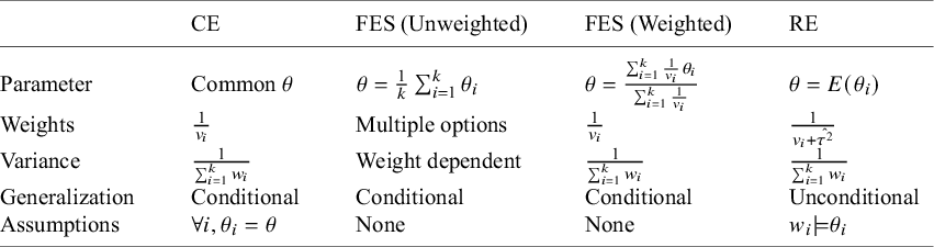


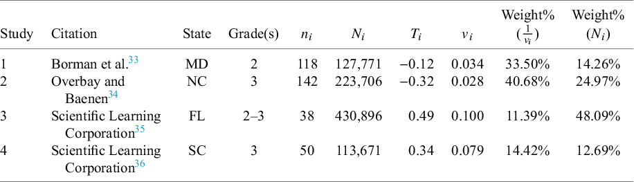
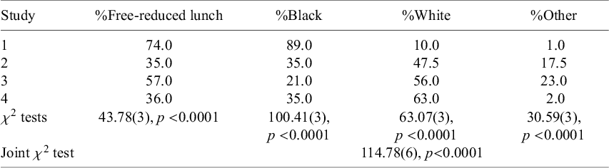
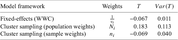
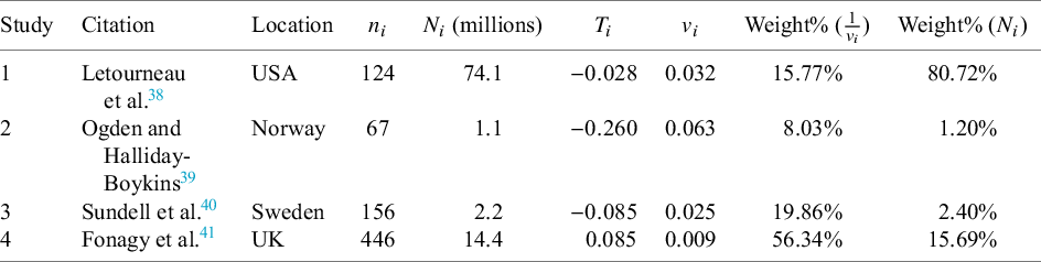
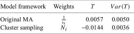

 Open access

