1 Introduction
1.1 Motivation
A central problem in number theory is to estimate exponential sums of the form
 $$\begin{align*}\sum_{n \leqslant X}f(n) \operatorname{e}(n\alpha), \end{align*}$$
where
 $f(n)$
is an arithmetic function,
 $\operatorname {e}(x) = \exp (2\pi i x)$
, and
 $\alpha \in \mathbb {R}$
. Typically, such sums exhibit intricate oscillatory behavior that can be exploited to derive significant arithmetic results. A prominent example in this context is Vinogradov’s famous estimate for exponential sums over primes. Let
 $\alpha \in \mathbb {R}$
and consider a reduced fraction
 $a/q$
such that
 $|\alpha -a / q| \leqslant 1 / q^2$
. Expanding upon the work of Vinogradov [Reference Vinogradov34], Vaughan [Reference Vaughan30] showed that for all
 $X \geqslant 2$
, we have
 $$ \begin{align} \sum_{n \leqslant X} \Lambda(n) \operatorname{e}(n \alpha) \ll\left(X^{4 / 5}+\frac{X}{q^{1/2}}+X^{1/2}q^{1/2}\right)(\log X)^{5 / 2}, \end{align} $$
where
 $\Lambda (n)$
is the Von-Mangoldt function. Indeed, the estimate (1.1) is crucial in bounding minor arc contributions in the Hardy–Littlewood circle method corresponding to the ternary Goldbach problem.
Our primary aim in this paper is to prove results on exponential sums involving generalized Möbius functions and their convolutions. As an application, we establish asymptotic formulas for certain weighted chromatic partitions by using the Hardy–Littlewood circle method.
1.2 Main results
Consider the Möbius function denoted by
 $\mu $
, which is a multiplicative function defined in the following way: for each prime p,
 $$\begin{align*}\mu(p^k) := \begin{cases} -1, & k=1 \\ 0, & k \geqslant 2. \end{cases}\end{align*}$$
By definition,
 $\mu ^{2}(n)=1$
if n is squarefree and
 $\mu ^{2}(n)=0$
otherwise. Let us write
 $$ \begin{align*} S_{\mu}(X, \alpha) =\sum_{n\leqslant X}\mu(n)\operatorname{e}(n\alpha). \end{align*} $$
Then, we have the following result.
Theorem 1.1 Let
 $\alpha \in \mathbb {R}$
and consider a reduced fraction
 $a/q$
such that
 $|\alpha -a/q|\leqslant 1/q^2$
. Then, for
 $X \geqslant 2$
and for any fixed
 $\varepsilon>0$
, we have
 $$ \begin{align*} S_{\mu}(X, \alpha) \ll_{\varepsilon} X^{4/5+\varepsilon}+ \dfrac{X(\log X)^3}{q^{1/2}} + X^{1/2}q^{1/2}(\log X)^3. \end{align*} $$
More generally, for any positive integer k, we define the Popovici-Möbius function (see [Reference Sándor and Crstici28, §2.2] as well as [Reference Calderón and Zárate4] and [Reference Kühn and Robles19, Reference Robles and Roy26] for related applications) with parameter k by
 $$ \begin{align} \mu_k(n) := (\mu * \mu * \cdots * \mu)(n), \end{align} $$
where the Dirichlet convolution is performed k times. The Dirichlet series for
 $\mu _k(n)$
is given by
 $$ \begin{align*} \sum_{n=1}^\infty \frac{\mu_k(n)}{n^s} = \frac{1}{\zeta(s)^k}, \end{align*} $$
for
 $\operatorname {Re}(s)> 1$
. Let
 $$ \begin{align*} S_{\mu_k}(X, \alpha) =\sum_{n\leqslant X }\mu_k(n)\operatorname{e}(n\alpha). \end{align*} $$
We prove the following theorem.
Theorem 1.2 Let
 $\alpha \in \mathbb {R}$
and consider a reduced fraction
 $a/q$
such that
 $|\alpha -a/q|\leqslant 1/q^2$
. Consider the sequences
 $\{a_m\}, \{b_m\}$
, and
 $ \{c_m\}$
given by
 $$ \begin{align*} a_1 &= \frac{4}{5} \quad \textrm{and} \quad \hspace{0.35cm}a_{m+1} = \frac{4-a_m}{5-2a_m} \quad \textrm{for} \quad m=1,2,\ldots, \\ b_1 &= \frac{1}{2} \quad \textrm{and} \quad \quad b_{m+1} = \frac{b_m}{3} \quad \quad \quad \hspace{0.05cm} \textrm{for} \quad m=1,2,\ldots, \\ \textrm{as well as} \quad c_1 &= \frac{1}{2} \quad \textrm{and} \quad \quad c_{m+1} = \frac{4-c_m}{5-2c_m} \quad \textrm{for} \quad m=1,2,\ldots. \end{align*} $$
Then, for
 $X \geqslant 2$
,
 $k \geqslant 2$
and any fixed
 $\varepsilon>0$
, we have
 $$ \begin{align*} S_{\mu_k}(X, \alpha) \ll_{\varepsilon} X^{a_k+\varepsilon}+ \dfrac{X(\log X)^{k^2}}{q^{b_k}} + X^{c_k}q^{1-c_k}(\log X)^{k^2}. \end{align*} $$
We also establish results for exponential sums involving Dirichlet convolutions of the Möbius function with the characteristic function of squarefull and squarefree integers, respectively. To this end, we define the arithmetic function
 $\hat {\mu }$
by
 $$ \begin{align*} \hat{\mu}(n) := (\mu*f)(n), \end{align*} $$
where f denotes the indicator function for the squarefull numbers. Writing
 $$ \begin{align*} S_{\hat{\mu}}(X, \alpha) =\sum_{n\leqslant X }\hat{\mu}(n)\operatorname{e}(n\alpha), \end{align*} $$
we are able to prove the following estimate.
Theorem 1.3 Let
 $\alpha \in \mathbb {R}$
and consider a reduced fraction
 $a/q$
such that
 $|\alpha -a/q|\leqslant 1/q^2$
. Then, for
 $X \geqslant 2$
, we have
 $$ \begin{align*} S_{\hat{\mu}}(X, \alpha) \ll \bigg(X^{5/6} + q^{1/2}X^{1/2} + \dfrac{X}{q^{1/2}}\bigg)(\log X)^{5/2}. \end{align*} $$
Considering the convolution of the Möbius function with the characteristic function of squarefree integers, we define
 $\tilde {\mu }_k(n)$
in terms of coefficients of the following Dirichlet series. Let
 $k \geqslant 1$
and
 $$ \begin{align*} \sum_{n=1}^\infty\dfrac{\tilde{\mu}_k(n)}{n^s}=\dfrac{1}{\zeta(ks)}, \end{align*} $$
for
 $\operatorname {Re}(s)> 1/k$
. As an example, for
 $k=2$
, one has
 $\tilde {\mu }_2(n) = (\mu *\mu ^2)(n)$
, where
 $\mu ^2$
is the indicator function for the squarefrees. Our next result provides an upper bound for the exponential sum
 $$ \begin{align*} S_{\tilde{\mu}_2}(X, \alpha) = \sum_{n\leqslant X }\tilde{\mu}_2(n)\operatorname{e}(n\alpha). \end{align*} $$
Theorem 1.4 Let
 $\alpha \in \mathbb {R}$
and consider a reduced fraction
 $a/q$
such that
 $|\alpha -a/q|\leqslant 1/q^2$
. Then, for
 $X \geqslant 2$
, we have
 $$ \begin{align*} S_{\tilde{\mu}_2}(X, \alpha)\ll \bigg(X^{23/28} + \dfrac{X}{q^{1/4}} + X^{3/4}q^{1/4}\bigg)(\log X)^{10}. \end{align*} $$


1.3 Applications to partitions
A partition of a positive integer n is a nondecreasing sequence of positive integers whose sum is equal to n. The partition function
 $p(n)$
, which represents the number of partitions of n, was first studied by Hardy and Ramanujan [Reference Hardy and Ramanujan13] in 1918 by applying the Hardy–Littlewood circle method. Their result states that
 $$ \begin{align*} p(n) \sim \frac{1}{4n\sqrt{3}} \exp \bigg(\pi\sqrt{\frac{2n}{3}}\bigg) \quad \mathrm{as} \quad n \to \infty. \end{align*} $$
As an application of our results on exponential sums from Section 1.2, we consider a question about partitions of a positive integer that has a strong arithmetic flavor. To be precise, we look at the parts that appear in the partition, and more specifically, we consider the prime factorization of the parts. Let B (blue) and R (red) denote the set of squarefree numbers that have an even and, respectively, an odd number of prime factors. For the convenience of the reader, we use colors to show parity of these partitions. Thus, we write

We note in passing that the sets B and R are asymptotically just as numerous. Actually, it is expected that as x tends to infinity, the number of elements of B less than x differs from the number of elements of R less than x by at most
 $O_{\epsilon } (x^{1/2 + \epsilon })$
for any
 $\epsilon>0$
. As is well-known, this is equivalent to the Riemann hypothesis.
Definition 1.1 We call a partition of a positive integer n admissible if each part is either blue or red and each red part appears at most once. We say that an admissible partition is even (respectively odd) if the number of red parts used in the partitions is even (and respectively odd).
For example, there are exactly 15 admissible partitions in the case when
 $n=10$
. The partition

is not admissible because the red 2 appears twice. We see in Table 1.3 that there are
 $8$
even admissible partitions and
 $7$
odd admissible partitions in this situation. This naturally leads to the following question.

Question Is the number of even admissible partitions of n asymptotic to the number of odd admissible partitions of n as n tends to infinity?
We will address the above question as well as a more general version of this problem. To proceed, we start by considering the partition function
 $p_{w}(n)$
associated to a generating function of the form,
 $$ \begin{align} \Psi_{w}(z) = \sum_{n=1}^\infty p_{w}(n) z^n = \prod_{n \in \mathbb{N}} (1-z^n)^{-w(n)}, \quad \lvert z \rvert <1, \end{align} $$
where
 $w(n) \in \mathbb {Z}$
is the weight placed on each element
 $n \in \mathbb {N}$
. We refer to such partitions as weighted partitions. Our cases of interest will have weights given by the Möbius function (i.e.,
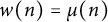 $w(n)=\mu (n)$
) or more generally by convolutions of the Möbius function (i.e.,
 $w(n) = \mu _{k}(n)$
, where
 $\mu _k(n)$
is defined by (1.2)).
In [Reference Vaughan32], Vaughan established an asymptotic formula for the number of partitions of a number n into primes when n is large by applying the Hardy-Littlewood circle method. In [Reference Vaughan33], Vaughan then extended this approach to study partition asymptotics regarding squares and other additive questions.
Since the publication of [Reference Vaughan32, Reference Vaughan33], there has been considerable interest in the study of restricted or weighted partitions over arithmetically interesting sets. In [Reference Gafni11], Gafni showed an asymptotic formula for the number of partitions of n into k-th powers, and in [Reference Gafni12], Gafni proved results for partitions into prime powers. Berndt, Malik, and the third author [Reference Berndt, Malik and Zaharescu2] studied partitions into k-th powers in arithmetic progressions. Dunn and the second author [Reference Dunn and Robles10] then considered the more general case where the parts are values of an arbitrary polynomial f of degree
 $d \ge 2$
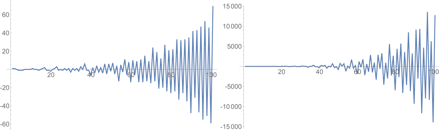
. More recently, Das, Berndt, Zeindler, and the second and third authors [Reference Berndt, Robles, Zaharescu and Zeindler3, Reference Das, Robles, Zaharescu and Zeindler8, Reference Robles and Zeindler27] studied partitions associated to generalized divisor functions, partitions into semiprimes and almost primes. General strategies for dealing with asymptotic weighted partitions have been established by Meinardus [Reference Meinardus21] and more recently by Debryune and Tenenbaum [Reference Debryune and Tenenbaum9]. Notice that in the case of the above-mentioned results, the corresponding partitions have nonnegative weights, unlike our cases of interest where the weights take positive and negative values (see Figure 1.2). In our cases, one should be prepared in principle to have a main result which is an upper bound rather than an asymptotic formula. This indeed happens in our case, see Theorem 1.6 below.
Very recently, in [Reference Daniels5, Reference Daniels6], Daniels investigated partitions whose generating functions are given by
 $$ \begin{align} \Psi(z,f) = 1 + \sum_{n=1} p(n,f) z^n = \prod_{n=1}^\infty (1- f(n)z^n)^{-1}, \quad \lvert z \rvert <1. \end{align} $$
Daniels refers to such partitions as signed partitions. In particular, he studied the case when
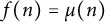 $f(n) = \mu (n)$
. Note the difference between placing
 $\mu (n)$
in the exponent of the factor
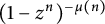 $(1-z^n)^{-\mu (n)}$
in (1.3) as opposed to the presence of
 $\mu (n)$
inside the factor
 ${(1-\mu (n)z^n)^{-1}}$
in (1.4). This is a subtle difference, which surprisingly leads to the existence of main terms in Daniel’s works and the non-existence of main terms in our context. For comparison, the reader is referred to Theorem 1.1 in [Reference Daniels5] and Theorem 1.6 below. We remark that Theorem 1.6 below does lead to an asymptotic formula connecting the number of odd and even admissible partitions as in Definition 1.1.
It is straightforward to see that in the particular case when
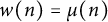 $w(n)= \mu (n)$
, the partition function
 $p_{\mu }(n)$
is exactly the difference between the number of even admissible partitions and odd admissible partitions of n as in Definition 1.1. More precisely, suppose we denote by
 $\mathcal {A}(n)$
the number of admissible partitions of n. Additionally, let
 $\mathcal {E}(n)$
and
 $\mathcal {O}(n)$
be the number of even and odd admissible partitions of n, respectively. Then,
 $$ \begin{align} \qquad\ \ p_{\mu}(n) &= \mathcal{E}(n)-\mathcal{O}(n), \end{align} $$
 $$ \begin{align} \textrm{and} \quad \mathcal{A}(n) &= \mathcal{E}(n)+\mathcal{O}(n). \end{align} $$
Therefore, in order to show that the number of even admissible partitions is asymptotic to the number of odd admissible partitions as n tends to infinity, our goal in what follows is to provide an upper bound for their difference (i.e., for
 $p_{\mu }(n)$
). We begin by answering the question raised previously in this section.
Theorem 1.5 The number of odd admissible partitions of n is asymptotic to the number of even admissible partitions of n, as n tends to infinity.
More generally, for any positive integer k, let
 $p_{\mu _k}(n)$
be the number of partitions of n weighted by
 $\mu _k(n)$
; that is,
 $$ \begin{align*} \sum_{n=1}^\infty p_{\mu_k}(n) z^n = \prod_{n=1}^\infty (1-z^n)^{-\mu_k(n)}, \end{align*} $$
where
 $\mu _k(n)$
is defined by (1.2). For simplicity, we will focus only on the case when
 $k=2$
. This is more involved than the case when
 $k=1$
and already demonstrates all the ingredients necessary for a general k. For
 $k=2$
, we prove the following result.
Theorem 1.6 For any fixed
 $B>0$
and for all
 $n \geqslant 2$
, we have
 $$ \begin{align} \log p_{\mu*\mu}(n) = O_B\left ( \frac{\sqrt{n}}{(\log n)^B} \right). \end{align} $$
Remark 1.2 As we shall see in the proof of Theorem 1.6, the method can be generalized to any
 $k \geqslant 1$
, with the same upper bound as in (1.7). In particular, when
 $k=1$
, we have
 $$ \begin{align} \log p_{\mu}(n) = O_B\left ( \frac{\sqrt{n}}{(\log n)^B} \right), \end{align} $$
for any fixed
 $B>0$
and all
 $n \geqslant 2$
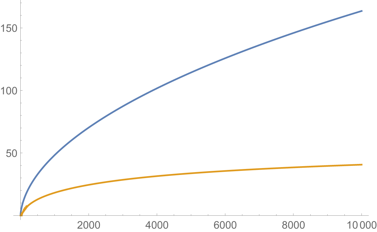
. Theorem 1.5 is an immediate consequence of (1.5) and (1.8). See Figure 1.1 for a plot of the logarithms of
 $\mathcal {A}(n)$
and
 $ p_{\mu }(n)$
.
Plot of
 $\log \mathcal {A}(n)$
in blue and
 $\log {p}_{\mu }(n)$
in orange for
 $1 \leqslant n \leqslant 10000$
.

 $ \underline {\mathrm {Left}}$
: Plot of partition function
 $p_w(n)$
with
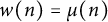 $w(n) = \mu (n)$
,
 $ \underline {\mathrm {Right}}$
: Plot of partition function
 $p_w(n)$
with
 $w(n) = (\mu *\mu )(n)$
.

Remark 1.3 It would be interesting to see what the analogues of Theorems 1.5 and 1.6 are if the Möbius function
 $\mu (n)$
is replaced by the Liouville function
 $\lambda (n)$
, where
 $$\begin{align*}\lambda(n) = \prod_{i=1}^{k} (-1)^{a_i}, \quad \textrm{where} \quad n = \prod_{i=1}^{k} p_i^{a_i}. \end{align*}$$
In order to prove Theorem 1.6, we will employ the Hardy-Littlewood method. As we shall see in Section 8, the contribution from the major arcs is closely related to the zeros of the Riemann zeta-function
 $\zeta (s)$
. To be precise, following (1.3), let us write
 $$ \begin{align} \Psi_{\mu*\mu}(z) = \sum_{n=1}^\infty p_{\mu*\mu}(n) z^n = \prod_{n=1}^\infty (1-z^n)^{-(\mu*\mu)(n)}, \quad \lvert z \rvert <1. \end{align} $$
Set
 $$ \begin{align} \Phi_{\mu*\mu}(z) := \sum_{j=1}^\infty \sum_{n=1}^\infty \frac{(\mu*\mu)(n)}{j} z^{jn}, \quad \lvert z \rvert <1. \end{align} $$
Then,
 $\Psi _{\mu *\mu }(z) = \exp (\Phi _{\mu *\mu }(z))$
. Let
 $X \geqslant 1$
and
 $\rho = \exp (-1/X)$
. Choose
 $z = \rho \operatorname {e}(\theta )$
in (1.10) and let
 $$\begin{align*}\Delta := \frac{1}{(1+4\pi^2X^2\theta^2)^{1/2}}. \end{align*}$$
Then we have the following theorem.
Theorem 1.7 Suppose that
 $\theta \in \mathbb {R}$
and
 $X \geqslant 1$
. If
 $X \Delta ^3 \geqslant 1$
, then there exists a sequence
 $T_{\nu }$
with
 $\nu \leqslant T_\nu \leqslant 2\nu$
such that
 $$ \begin{align} \Phi_{\mu * \mu}(\rho \operatorname{e}(\theta)) &= 4 \log \frac{X}{1-2\pi i X\theta} - 8 \log(2 \pi) + 72 \frac{1-2\pi i X\theta}{X}\nonumber \\ & \quad + \lim_{\nu \to \infty} \sum_{|\operatorname{Im}(\varpi)| < T_\nu} f(X,\theta,\varpi) +\sum_{n=1}^{\infty} g(X,\theta,n), \end{align} $$
where the functions f and g in (1.11) are given by
 $$ \begin{align*} f(X, \theta, \varpi) &:= \bigg(\frac{X}{1-2\pi i X\theta}\bigg)^{\varpi}\frac{\zeta (1 + \varpi )\Gamma (\varpi )}{{\zeta '{{(\varpi )}^2}}} \bigg(\log \frac{X}{1-2\pi i X\theta} + \psi (\varpi ) - \frac{{\zeta "}}{{\zeta '}}(\varpi ) + \frac{{\zeta '}}{\zeta }(1 + \varpi ) \bigg), \\ g(X,\theta,n) &:= \bigg(\frac{X}{1-2\pi i X\theta}\bigg)^{-2 n} \bigg[\mathfrak{c}_1(n) \bigg(\log \frac{X}{1-2\pi i X\theta}\bigg)^2 + \mathfrak{c}_2(n) \log \frac{X}{1-2\pi i X\theta}+ \mathfrak{c}_3(n) \bigg]. \end{align*} $$
The coefficients
 $\mathfrak {c}_1(n), \mathfrak {c}_2(n)$
, and
 $\mathfrak {c}_3(n)$
are defined in (8.3), (8.4), and (8.5), respectively. The sum is taken over the nontrivial zeros
 $\varpi $
of
 $\zeta (s)$
under the assumption, for notational ease, of simplicity.
Remark 1.4 As Titchmarsh puts it in [Reference Titchmarsh29, §14.27], “obvious modifications are required if” the zeros are not simple. Indeed, this assumption does not represent a technical difficulty, and it can be relaxed at the expense of cluttering the expression
 $f(X,\theta ,\varpi )$
for the nontrivial zeros.
Remark 1.5 Interestingly, (1.11) is an instance of an explicit formula in the theory of partitions. It is reminiscent of the classical explicit formula
 $$ \begin{align*} \psi_0(x) = \frac{1}{2} \lim_{\delta \to 0} (\psi(x+\delta)-\psi(x-\delta)) = x - \lim_{T \to \infty}\sum_{\lvert \operatorname{Im}(\varpi) \rvert <T} \frac{x^\varpi}{\varpi} - \log(2\pi) + \sum_{n=1}^{\infty} \frac{x^{-2n}}{2n}. \end{align*} $$
Here,
 $\varpi $
runs over the nontrivial zeros of
 $\zeta (s)$
and
 $$ \begin{align} \psi(x) = \sum_{p^k \leqslant x} \log p, \end{align} $$
where the sum in (1.12) is over prime powers.
Remark 1.6 Consider the truncated arithmetic sum
 $$ \begin{align*} \Phi_1 := \Phi_{1}(X,\theta, J, N) = \sum_{j=1}^J \sum_{n=1}^N \frac{(\mu * \mu)(n)}{j} \exp\bigg( -jn \bigg(\frac{1}{X}-2\pi i \theta\bigg)\bigg) \end{align*} $$
and its analytic truncated counterpart
 $$ \begin{align*} \Phi_2 := \Phi_{2}(X,\theta,T,N) &= 4 \log \frac{X}{1-2\pi i X\theta} - 8 \log(2 \pi) + 72 \frac{1-2\pi i X\theta}{X} \\ &\quad+ \sum_{\lvert \operatorname{Im}(\varpi) \rvert < T} f(X,\theta,\varpi) +\sum_{n=1}^{N} g(X,\theta,n). \end{align*} $$
We set
 $\theta =\theta (X)$
as
 $$ \begin{align*} \theta(X) := \frac{1}{2\pi} \sqrt{\frac{1}{X^{4/3}}-\frac{1}{X^2}}, \end{align*} $$
such that
 $X \Delta ^3=1$
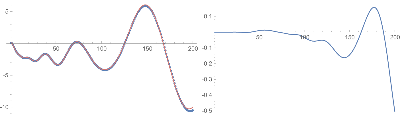
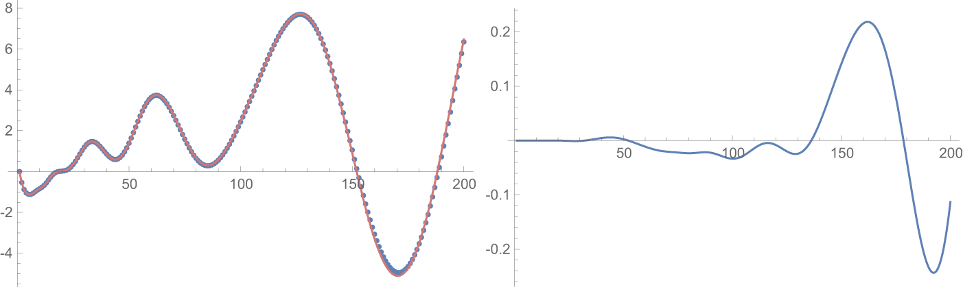
. In Figures 1.3 and 1.4, we numerically illustrate our result from Theorem 1.7 in terms of the functions
 $\Phi _1$
and
 $\Phi _2$
.
 $ \underline {\mathrm {Left}}$
: Plot of
 $\operatorname {Re}(\Phi _1(X,\theta ,120,800))$
in blue and
 $\operatorname {Re}(\Phi _2(X,\theta ,20,10))$
in pink.
 $ \underline {\mathrm {Right}}$
: Plot of
 $\operatorname {Re}(\Phi _1(X,\theta ,120,800))-\operatorname {Re}(\Phi _2(X,\theta ,20,10))$
.

 $ \underline {\mathrm {Left}}$
: Plot of
 $\operatorname {Im}(\Phi _1(X,\theta ,120,800))$
in blue and
 $\operatorname {Im}(\Phi _2(X,\theta ,20,10))$
in pink.
 $ \underline {\mathrm {Right}}$
: Plot of
 $\operatorname {Im}(\Phi _1(X,\theta ,120,800))-\operatorname {Im}(\Phi _2(X,\theta ,20,10))$
.

1.4 Structure of the paper
The paper is organized as follows. In Section 2, we introduce some preliminary lemmas, such as Type I and Type II estimates on exponential sums involving Dirichlet convolutions, a result on the distribution of the Möbius function in arithmetic progressions, a divisor sum estimate, and an unconditional upper bound on
 $1/\zeta (s)$
in the critical strip along specific vertical line segments. Section 3 is devoted to the proofs of Theorems 1.1, 1.3, and 1.4. The proof of Theorem 1.2 is singled out in Section 4. In Section 5, we move on to the theory of partitions and set up the proof of Theorem 1.6. Section 6 and Section 7 will contain the details of the major and minor arc estimates, respectively. Finally, in 8, we present the proof of Theorem 1.7.
2 Preliminary Lemmas
In this section, we start by establishing some standard notations. Then, we collect some necessary results from the literature and proceed to prove some preliminary lemmas.
2.1 Notations
We employ some standard notation that will be used throughout the paper.
-
• Throughout the paper, the expressions
 $f(X)=O(g(X))$
,
$f(X) \ll g(X)$
, and
$g(X) \gg f(X)$
are equivalent to the statement that
$|f(X)| \leq C|g(X)|$
for all sufficiently large X, where
$C>0$
is an absolute constant. A subscript of the form
$\ll _{\alpha }$
means the implied constant may depend on the parameter
$\alpha $
. Dependence on several parameters is indicated in an analogous manner, as in
$\ll _{\alpha , \lambda }$
.
-
• The notation
$f = o(g)$
as
$x\to a$
means that
$\lim _{x\to a} f(x)/g(x) = 0$
and
$f\sim g$
as
${x\to a}$
denotes
$\lim _{x\to a} f(x)/g(x)= 1$
. -
• We denote the set of real numbers by
$\mathbb {R}$
, the set of rational numbers by
$\mathbb {Q}$
, the set of integers by
$\mathbb {Z}$
, the set of natural numbers by
$\mathbb {N}$
, and the set of complex numbers by
$\mathbb {C}$
. -
• For any set
$\mathcal {A}$
,
$\operatorname {card}(\mathcal {A})$
denotes the cardinality of the set
$\mathcal {A}$
. -
• The notation
$\operatorname {e}(x)$
stands for
$\exp (2\pi i x)$
. -
• Dyadic sums are represented by
$\sum _{n \sim N} f(n) = \sum _{N < n \leqslant 2N} f(n)$
. -
• The divisor function is denoted by
$\tau (n)$
. The k-fold divisor function
$\tau _k(n)$
is defined by the coefficients of the Dirichlet series
$$\begin{align*}\zeta^k(s) = \sum_{n=1}^{\infty}\frac{\tau_k(n)}{n^s}, \quad \textrm{for } \operatorname{Re}(s)> 1. \end{align*}$$
-
• The Möbius function is denoted by
$\mu (n)$
, whereas the Popovici-Möbius function will be denoted by
$\mu _k(n) = (\mu * \mu *\cdots * \mu )(n)$
, the convolution performed k times. -
• We denote by
$\hat {\mu }$
the convolution of the Möbius function with the characteristic function of the squarefull numbers. More precisely, we write where f denotes the indicator function for the squarefull numbers.
$$ \begin{align*} \hat{\mu}(n) := (\mu*f)(n), \end{align*} $$
-
• The arithmetic function
$\tilde \mu _k(n)$
is defined by the coefficients of the Dirichlet series for
$$\begin{align*}\sum_{n \geqslant 1} \frac{\tilde \mu_k(n)}{n^s} = \frac{1}{\zeta(ks)} \end{align*}$$
$\operatorname {Re}(s)>\frac {1}{k}$
.


















2.2 Exponential sums and Dirichlet convolutions
We first state the following two lemmas, due to Koukoulopoulos, that provide bounds on exponential sums involving Dirichlet convolutions.
Lemma 2.1 (Type I estimate)
Let
 $f\colon \mathbb {N}\to \mathbb {C}$
be supported on
 $[1, y]$
,
 $v\geqslant 2$
,
 $X\geqslant 2$
,
 $\alpha \in \mathbb {R}$
and
 $a/q$
be a reduced fraction such that
 $|\alpha -a/q|\leqslant 1/q^2$
. Then,
 $$ \begin{align*} \sum_{n\leqslant X}(f*\log^v)(n)\operatorname{e}(n\alpha)\ll \bigg(y + \dfrac{X}{q}+q\bigg)(\log X)^{v+1}\|f\|_{\infty}. \end{align*} $$
Proof See [Reference Koukoulopoulos16, Theorem 23.5].
Lemma 2.2 (Type II estimate)
Let
 $f, g\colon \mathbb {N}\to \mathbb {C}$
be two arithmetic functions supported on
 $[1, y]$
and
 $[1, z]$
, respectively. Let
 $X\geqslant 2$
,
 $\alpha \in \mathbb {R}$
and consider a reduced fraction
 $a/q$
such that
 $|\alpha -a/q|\leqslant 1/q^2$
. Then,
 $$ \begin{align*} \sum_{n\leqslant X}(f*g)(n)\operatorname{e}(n\alpha)\ll \bigg(q + y +z + \dfrac{yz}{q}\bigg)^{1/2}\sqrt{\log 2q}\cdot \|f\|_2\|g\|_2. \end{align*} $$
Proof See [Reference Koukoulopoulos16, Theorem 23.6].
We would like to establish more general versions of Lemmas 2.1 and 2.2, in the case when
 $\alpha \in \mathbb {R}$
and there exists some reduced fraction
 $a/q$
such that
 $|\alpha -a/q|\leqslant \gamma /q^2$
, for some
 $\gamma \geqslant 1$
. In this regard, we first prove the following proposition.
Proposition 2.1 Let
 $\alpha \in \mathbb {R}$
and consider a reduced fraction
 $a/q$
such that
 $|\alpha -a/q|\leqslant \gamma /q^2$
for some
 $\gamma \geqslant 1$
. Then, for each
 $m_1 \in \{1,2,\dots ,q\}$
, there exists at most
 $14 \gamma $
choices of
 $m_2 \in \{1,2,\dots ,q \}$
such that
 $$ \begin{align} \bigg \lvert \left\lVert m_1\alpha\right\rVert- \left\lVert m_2\alpha\right\rVert \bigg \rvert < \frac{1}{q}, \end{align} $$
where
 $\left \lVert x\right \rVert $
denotes the smallest distance of x to an integer.
Proof Fix
 $m_1 \in \{1,2,\dots , q\}$
and suppose
 $m_2 \in \{1,2\dots ,q\}$
such that (2.1) is satisfied. Writing
 $\alpha =a/q+\beta $
with
 $\lvert \beta \rvert \leqslant \gamma /q^2$
, we have
 $$\begin{align*}m_1 \alpha = \frac{m_1a}{q}+m_1\beta \quad \textrm{ and} \quad m_2 \alpha = \frac{m_2a}{q}+m_2\beta. \end{align*}$$
Therefore, we obtain
 $$ \begin{align} \bigg \lvert \left\lVert m_1\alpha\right\rVert- \left\lVert\frac{m_1 a}{q}\right\rVert \bigg \rvert \leqslant\lvert m_1\beta \rvert \leqslant\frac{\gamma}{q} \quad \mathrm{and} \quad \bigg \lvert \left\lVert m_2\alpha\right\rVert- \left\lVert\frac{m_2 a}{q}\right\rVert \bigg \rvert \leqslant\lvert m_2\beta \rvert \leqslant\frac{\gamma}{q}. \end{align} $$
From (2.1) and (2.2), it follows that
 $$ \begin{align} \bigg \lvert \left\lVert\frac{m_1 a}{q}\right\rVert- \left\lVert\frac{m_2 a}{q}\right\rVert \bigg \rvert \leqslant \frac{2\gamma+1}{q} \leqslant\frac{3\gamma}{q}. \end{align} $$
Next, we write
 $$\begin{align*}\left\lVert\frac{m_1 a}{q}\right\rVert = \frac{\ell_1}{q} \quad \mathrm{and} \quad \left\lVert\frac{m_2 a}{q}\right\rVert = \frac{\ell_2}{q}, \end{align*}$$
where
 $\ell _1, \ell _2 \in \{0,1,\dots ,\lfloor q/2\rfloor \}$
. Note that when
 $m_1$
is fixed,
 $\ell _1$
is fixed. Also, for each choice of
 $\ell _2$
, there are at most two different choices of
 $m_2$
. Hence, in order to satisfy (2.3), there are at most
 $7\gamma $
choices of
 $\ell _2$
. This implies there are at most
 $14 \gamma $
choices of
 $m_2$
which satisfy (2.1).
With Proposition 2.1 in hand, we have the following two lemmas.
Lemma 2.3 Let
 $f\colon \mathbb {N}\to \mathbb {C}$
be supported on
 $[1, y]$
,
 $v\geqslant 2$
,
 $X\geqslant 2$
,
 $\alpha \in \mathbb {R}$
and
 $a/q$
be a reduced fraction such that
 $|\alpha -a/q|\leqslant \gamma /q^2$
for some
 $\gamma \geqslant 1$
. Then,
 $$ \begin{align} \sum_{n\leqslant X}(f*\log^v)(n)\operatorname{e}(n\alpha)\ll \gamma \bigg(y + \dfrac{X}{q}+q\bigg)(\log x)^{v+1}\|f\|_{\infty}, \end{align} $$
where the implied constant in (2.4) is absolute.
Lemma 2.4 Let
 $f, g\colon \mathbb {N}\to \mathbb {C}$
be two arithmetic functions supported on
 $[1, y]$
and
 $[1, z]$
, respectively. Let
 $X\geqslant 2$
,
 $\alpha \in \mathbb {R}$
and consider a reduced fraction
 $a/q$
such that
 $|\alpha -a/q|\leqslant \gamma /q^2$
for some
 $\gamma \geqslant 1$
. Then,
 $$ \begin{align} \sum_{n\leqslant X}(f*g)(n)\operatorname{e}(n\alpha)\ll \gamma \bigg(q + y +z + \dfrac{yz}{q}\bigg)^{1/2}\sqrt{\log 2q}\cdot \|f\|_2\|g\|_2, \end{align} $$
where the implied constant in (2.5) is absolute.
We only prove Lemma 2.3. The proof of Lemma 2.4 is similar.
Proof of Lemma 2.3
Following the proof of Theorem 23.5 in [Reference Koukoulopoulos16], it suffices to bound the sum
 $$\begin{align*}\sum_{k \leqslant y} \min \bigg \{\frac{X}{k},\frac{1}{\left\lVert k\alpha\right\rVert} \bigg \}. \end{align*}$$
To do so, we divide the interval
 $[1,y]$
into subintervals of length q and write
 $$ \begin{align*}S_m:=\sum_{m q<k \leqslant(m+1) q} \min \bigg \{\frac{X}{k},\frac{1}{\left\lVert k\alpha\right\rVert} \bigg \}. \end{align*} $$
Note that
 $$\begin{align*}\sum_{k \leqslant y} \min \bigg \{\frac{X}{k},\frac{1}{\left\lVert k\alpha\right\rVert} \bigg \} \leqslant\sum_{m=0}^{\lfloor y/q \rfloor} S_m. \end{align*}$$
We write
 $\alpha =a/q+\beta $
with
 $\lvert \beta \rvert \leqslant \gamma /q^2$
and consider two cases.
Case 1:
 $m \geqslant 1$
. Writing
 $k=mq+r$
where
 $1 \leqslant r \leqslant q$
, we have
 $ \left \lVert k\alpha \right \rVert = \left \lVert r\alpha +mq\beta \right \rVert $
. Define the intervals
 $$\begin{align*}I _j = \bigg [\frac{j-1}{2q}, \frac{j}{2q}\bigg ), \quad j \in \{1,2,\dots, \lceil q \rceil \}. \end{align*}$$
Fix some
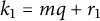 $k_1=mq+r_1$
, such that
 $ \left \lVert k_1\alpha \right \rVert \in I _j$
for some j. Since
 $I _j$
is an interval of length
 $1/2q$
, it follows that
 $\left \lVert r_1\alpha \right \rVert $
is contained in the union of at most two intervals, say
 $T_1$
and
 $T_2$
, each of length at most
 $1/2q$
. Suppose for some
 $k_2=mq+r_2$
,
 $ \left \lVert k_2\alpha \right \rVert \in I _j$
as well. Then,
 $\left \lVert r_2\alpha \right \rVert $
is also contained in
 $T_1 \cup T_2$
. But using Proposition 2.1, each of
 $T_1$
or
 $T_2$
can contain at most
 $14 \gamma $
choices of
 $r_2$
. Hence, there can be at most
 $28 \gamma $
different
 $k_2$
such that both
 $\left \lVert k_1 \alpha \right \rVert $
and
 $\left \lVert k_2 \alpha \right \rVert $
lie in
 $I _\ell $
. Therefore, the contribution from those k’s for which
 $\left \lVert k \alpha \right \rVert \in I _j$
to the sum
 $S_m$
is
 $$\begin{align*}\leqslant\frac{60 \gamma q}{j-1}, \end{align*}$$
when
 $j>1$
. For the specific case when
 $j=1$
, we trivially bound the contribution by
 $30\gamma /mq$
. Therefore, for
 $m \geqslant 1$
, we obtain
 $$ \begin{align*}S_m \leqslant 30 \gamma \bigg (\frac{ X}{m q}+\sum_{2 \leqslant j \leqslant \lceil q \rceil } \frac{2 q}{j-1} \bigg) \ll \gamma \left (\frac{ X}{m q}+q \log q \right ). \end{align*} $$
Case 2:
 $m=0$
. For all
 $r \geqslant q/2\gamma $
, an argument similar to the previous case shows that the contribution from such terms is
 $\ll \gamma (X/q+q \log q)$
. Finally, we are left with the cases when
 $r<q/2\gamma $
. Then,
 $\lvert r \beta \rvert \leqslant 1/2q$
, which implies
 $\left \lVert r \alpha \right \rVert \geqslant 1/2q$
. Therefore, the total contribution from the cases when
 $r < q/2\gamma $
is
 $$\begin{align*}\ll \gamma(2q+q \log q) \ll \gamma q \log q. \end{align*}$$
The rest of the proof follows along the lines of the proof of [Reference Koukoulopoulos16, Theorem 23.5], and noting that there are
 $\ll y/q$
choices of m.
2.3 Exponential sums and the divisor function
We record the following result achieved by Mikawa that provides bounds on exponential sums involving the three-fold divisor function.
Lemma 2.5 Let
 $\alpha \in \mathbb {R}$
and consider a reduced fraction
 $a/q$
such that
 $|\alpha -a/q|\leqslant 1/q^2$
. Then, for
 $0<M$
,
 $J\leqslant X $
, we have
 $$\begin{align*}\sum_{m\sim M}\sum_{j\sim J}\tau_{3}(j)\min\bigg(\frac{X}{m^{2}j},\frac{1}{\Vert\alpha m^{2}j\Vert}\bigg) \ll MJ(\log X)^{3}+\dfrac{X^{3/4}}{M}\bigg(Xq^{-1}+XM^{-1}+q\bigg)^{1/4}(\log X)^{8},\end{align*}$$
where
 $\tau _3$
denotes the three-fold divisor function.
Proof See [Reference Mikawa22].
2.4 The Möbius function in arithmetic progressions
We collect below a result on the Möbius function in arithmetic progressions, due to Davenport, which is an application of the Siegel-Walfisz theorem with the standard zero-free region for Dirichlet L-functions.
Lemma 2.6 Let
 $X\geqslant 2$
and
 $B>0$
. Let
 $r, q\geqslant 1$
be two integers with
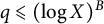 $q\leqslant (\log X)^B$
. Then, there exists a constant
 $c_B>0$
depending only on B such that
 $$ \begin{align*} \sum_{\substack{n \leqslant X \\ n \equiv r \operatorname{mod} q}} \mu(n) \ll_B X\exp(-c_B\sqrt{\log X}). \end{align*} $$
Proof See [Reference Davenport7, Lemma 6].
2.5 A divisor sum estimate
Let
 $k \in \mathbb {N}$
and let
 $\tau _k(n)$
be the k-fold divisor function. Norton established the following result.
Lemma 2.7 For
 $X \geqslant 1$
, and
 $k, r \geqslant 2$
, we have
 $$ \begin{align*} \sum_{n \leqslant X } (\tau_k(n))^r \ll X(\log X)^{k^r-1}. \end{align*} $$
Proof See [Reference Norton24, Eq. 1.10].
2.6 Bounding
$1/\zeta (s)$
in the critical strip.

In order to prove the explicit formula in Section 8, we will require a contour integration involving the term
 $1/\zeta ^2(s)$
. To prove our results unconditionally, we shall use the following result due to works of Ramachandra and Sankaranarayanan, and Inoue, which provide unconditional upper bounds for
 $1/\zeta (s)$
inside the critical strip along a specific vertical line segment.
Lemma 2.8 Let
 $T>0$
be a sufficiently large positive number and
 $H=T^{1/3}$
. Then, one has
 $$ \begin{align*} \min_{T \leqslant t \leqslant T+H} \max_{\frac{1}{2} \leqslant \sigma \leqslant 2} |\zeta(\sigma+it)|^{-1} \leqslant \exp( C (\log \log T)^2) \end{align*} $$
with an absolute constant
 $C>0$
. In particular, there exists a real
 $T_* \in [T,T+T^{1/3}]$
such that
 $$ \begin{align*} \frac{1}{\zeta(\sigma+iT_*)} \leqslant T_*^\varepsilon \quad \mathrm{where} \quad \frac{1}{2} \leqslant \sigma \leqslant 2, \end{align*} $$
for any
 $\varepsilon>0$
.
Proof See [Reference Ramachandra and Sankaranarayanan25, Theorem 2] and [Reference Inoue14, Lemma 1].
3 Proofs of Theorems 1.1, 1.3, and 1.4
In this section, we present the proofs of Theorems 1.1, 1.3, and 1.4.
3.1 Proof of Theorem 1.1
We can assume
 $q \leqslant X$
; otherwise, the conclusion follows trivially. Let
 $U, V \geqslant 2$
be parameters to be chosen later on. Applications of the Möbius inversion formula yield
 $$ \begin{align} \mu(n) &= \mu_{\leqslant U}(n) + \mu_{\leqslant V}(n)+ (\mu_{>U}*\mu_{>V}*1)(n) -(\mu_{\leqslant U}*\mu_{\leqslant V}*1)(n) \notag \\ & = \mu^{(1)} + \mu^{(2)}+\mu^{(3)}-\mu^{(4)}, \end{align} $$
say. Consider
 $\mu ^{(1)}$
and
 $\mu ^{(2)}$
first. Since our choice of parameters U and V will be small compared to X, bounding trivially, we arrive at
 $$ \begin{align} \sum_{n\leqslant X }\mu^{(1)}(n)\operatorname{e}(n\alpha)&\ll U \end{align} $$
 $$ \begin{align} \sum_{n\leqslant X }\mu^{(2)}(n)\operatorname{e}(n\alpha)& \ll V. \end{align} $$
For
 $\mu ^{(3)}(n)$
, we will use Lemma 2.2. However, applying the lemma directly does not suffice our purpose. We consider breaking our range into dyadic intervals. By definition, we have
 $$ \begin{align*}\mu^{(3)}(n)=\sum_{\substack{k \ell=n \\ k>U, \ell >V}} \mu_{>U}(k) (\mu_{>V} * 1)(\ell). \end{align*} $$
To obtain better control of the support of the variables k and
 $\ell $
, we break the interval
 $(U, X/ V]$
into dyadic intervals
 $\left (2^{j-1}, 2^j\right ]$
, where
 $2^j \in (U, 2 X / V]$
. If
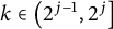 $k \in \left (2^{j-1}, 2^j\right ]$
, then
 $\ell =n / k \leqslant X / 2^{j-1}$
. With this more accurate decomposition, we have
 $$ \begin{align*}\mu^{(3)}(n)=\sum_{U<2^j \leqslant 2 X / V}\left(f_j * g_j\right)(n), \quad \text { for } n \leqslant X , \end{align*} $$
where
 $f_j(k)=\mu _{>U}(k) \cdot 1_{2^{j-1}<k \leqslant 2^j}$
and
 $g_j(\ell )=(\mu _{>V} * 1)(\ell ) \cdot 1_{V<\ell \leqslant X/ 2^{j-1}}$
. Then, applying Lemma 2.2, we obtain
 $$ \begin{align} \sum_{n\leqslant X }\mu^{(3)}(n)\operatorname{e}(n\alpha) &= \sum_{U<2^j \leqslant 2 X / V} \sum_{n\leqslant X }\left(f_j * g_j\right)(n)\operatorname{e}(n\alpha) \notag \\ &\ll \sum_{U<2^j \leqslant 2 X / V} \bigg(q^{1/2} + \dfrac{X^{1/2}}{U^{1/2}} +\dfrac{X^{1/2}}{V^{1/2}} + \dfrac{X^{1/2}}{q^{1/2}}\bigg)\sqrt{\log 2q}\cdot \|f_j\|_2\|g_j\|_2 \notag \\ &\ll \bigg(X^{1/2}q^{1/2} + \dfrac{X}{U^{1/2}} +\dfrac{X}{V^{1/2}}+ \dfrac{X}{q^{1/2}}\bigg)(\log X)^3. \end{align} $$
Note. In the rest of this section, we will always apply the above more accurate decomposition technique before applying Lemma 2.2.
Finally, we focus on
 $\mu ^{(4)}(n)$
. We apply Lemma 2.1 with
 $y=UV$
,
 $v=0$
, and
 ${f = \mu _{\leqslant U}*\mu _{\leqslant V}}$
. Since
 $\|f\|_{\infty } \ll _{\varepsilon } (UV)^{\varepsilon } $
for any fixed
 $\varepsilon>0$
, it follows that
 $$ \begin{align} \sum_{n\leqslant X }\mu^{(4)}(n)\operatorname{e}(n\alpha) \ll_{\varepsilon} (UV)^{\varepsilon}\bigg( UV+ \dfrac{X}{q} + q\bigg)(\log X). \end{align} $$
We choose
 $U=V=\min \{ X^{2/5}, q, X/q \}$
and combine the estimates (3.2), (3.3), (3.4), and (3.5) to obtain
 $$ \begin{align*} \sum_{n\leqslant X }\mu(n)\operatorname{e}(n\alpha) \ll_{\varepsilon} X^{4/5+\varepsilon}+ \dfrac{X(\log X)^3}{q^{1/2}} + X^{1/2}q^{1/2}(\log X)^3. \end{align*} $$
This ends the proof.
3.2 Proof of Theorem 1.3
The proof follows along the lines of the proof of Theorem 1.1. Again, we can assume
 $q \leqslant X$
. Let
 $U, V \geqslant 2$
be parameters to be chosen later on. Employing the Möbius inversion formula, we obtain
 $$ \begin{align*} \hat{\mu}(n)=\hat{\mu}_{ \leqslant U}(n) + (\hat{\mu}_{> U}*\mu_{>V}*1)(n) + (f*\mu_{\leqslant V})(n) - (\hat{\mu}_{ \leqslant U}*\mu_{\leqslant V}*1)(n). \end{align*} $$
Trivially, we have
 $$ \begin{align} \sum_{n\leqslant X }\hat{\mu}_{ \leqslant U}(n)\operatorname{e}(n\alpha) \ll U \log U. \end{align} $$
Next, by Lemma 2.2, similar to how we obtained (3.4), we have
 $$ \begin{align} \sum_{n\leqslant X } (\hat{\mu}_{> U}*\mu_{>V}*1)(n)\operatorname{e}(n\alpha) &\ll X^{1/2}\bigg(\dfrac{X}{U}+\dfrac{X}{V}+q + \dfrac{X}{q} \bigg)^{1/2} (\log X)^{5/2}\notag \\ &\ll \bigg(X^{1/2}q^{1/2}+\dfrac{X}{U^{1/2}}+\dfrac{X}{V^{1/2}} + \dfrac{X}{q^{1/2}}\bigg)(\log X)^{5/2}. \end{align} $$
Observing that
 $\|f \cdot 1_{n\leqslant X} \|_2 \ll X^{1/4}$
, again, an application of Lemma 2.2 shows that
 $$ \begin{align} \sum_{n\leqslant X }(f*\mu_{\leqslant V})(n)\operatorname{e}(n\alpha) &\ll \bigg(q + X + V + \dfrac{X}{q}\bigg)^{1/2}X^{1/4}V^{1/4}(\log X)^{3/2}\notag \\ &\ll \bigg(X^{1/4}V^{1/4}q^{1/2}+X^{3/4}V^{1/4}\bigg)(\log X)^{3/2}. \end{align} $$
Arguing as in the proof of (3.5) for the case of the Möbius function, we have
 $$ \begin{align} \sum_{n\leqslant X }(\hat{\mu}_{ \leqslant U}*\mu_{\leqslant V}*1)(n)\operatorname{e}(n\alpha) \ll_{\varepsilon} (UV)^{\varepsilon}\bigg( UV+ \dfrac{X}{q} + q\bigg)(\log X), \end{align} $$
for any fixed
 $\varepsilon>0$
. Finally, we choose
 $U=V=\min \{ X^{1/3}, q, X/q \}$
and combine (3.6), (3.7), (3.8), and (3.9) to obtain
 $$ \begin{align*} \sum_{n\leqslant X }\hat{\mu}(n)\operatorname{e}(n\alpha) \ll \bigg(X^{5/6} + q^{1/2}X^{1/2} + \dfrac{X}{q^{1/2}}\bigg)(\log X)^{5/2}, \end{align*} $$
which is the desired result.
3.3 Proof of Theorem 1.4
Similar to the previous proofs, we can assume
 $q \leqslant X$
. Let
 $U, V \geqslant 2$
be parameters to be chosen later on. We start with the following identity:
 $$ \begin{align*} \tilde{\mu}_2(n) &= \tilde{\mu}_2(n)\cdot 1_{n\leqslant U} + (\tilde{\mu}_2\cdot1_{n>U}*\mu_{>V}*1)(n) \notag \\ &\quad + (\mu^2*\mu_{\leqslant V})(n)-(\tilde{\mu}_2 \cdot 1_{n \leqslant U}*\mu_{\leqslant V}*1)(n). \end{align*} $$
Arguing as in the previous proofs, we can show that
 $$ \begin{align} \sum_{n\leqslant X }\tilde{\mu}_2(n)\cdot 1_{n \leqslant U} \operatorname{e}(n\alpha) &\ll U \log U, \end{align} $$
 $$ \begin{align} \sum_{n\leqslant X }(\tilde{\mu}_2\cdot1_{n>U}*\mu_{ >V}*1)(n)\operatorname{e}(n\alpha) &\ll \bigg(X^{1/2}q^{1/2} + \dfrac{X}{U^{1/2}}+\dfrac{X}{V^{1/2}} +\dfrac{X}{q^{1/2}}\bigg) (\log X)^3, \end{align} $$
 $$ \begin{align} \textrm{and} \quad \sum_{n\leqslant X }(\mu_{ \leqslant V}*\tilde{\mu}_2 \cdot 1_{n \leqslant U}*1)(n) \operatorname{e}(n\alpha) &\ll_{\varepsilon} (UV)^{\varepsilon}\bigg( UV+ \dfrac{X}{q} + q\bigg)(\log X), \end{align} $$
for any fixed
 $\epsilon>0$
. It remains to estimate the sum
 $$ \begin{align*} \sum_{n\leqslant X }(\mu^2*\mu_{\leqslant V})(n)\operatorname{e}(n\alpha). \end{align*} $$
A treatment like (3.8) is not enough in this case because
 $\|\mu ^2 \cdot 1_{n\leqslant X} \|_2 \ll X^{1/2}$
. Therefore, we proceed in a different way. Using the relation
 $\mu ^2(n)=\sum _{ab^2=n}\mu (b)$
, we can write
 $$ \begin{align} \sum_{n\leqslant X }(\mu^2*\mu_{\leqslant V})(n)\operatorname{e}(n\alpha) &=\sum_{\substack{mb^2\leqslant X \\ m\leqslant V}}\mu(b)\mu(m)\sum_{a\leqslant X /(mb^2)}\operatorname{e}(amb^2\alpha) \notag \\ &\ll \sum_{b\leqslant X ^{1/2}}\sum_{m\leqslant V}\min\bigg\{\dfrac{X}{b^2m}, \dfrac{1}{\|b^2m\alpha\|}\bigg\}. \end{align} $$
We need to break the range of b in (3.13) into two parts: for large b’s, we will use the bound from Lemma 2.5, and for small b’s, we will use the Cauchy-Schwarz inequality along with Lemma 2.1. Indeed, we write
 $$ \begin{align*} \sum_{b\leqslant X ^{1/2}}\sum_{m\leqslant V}\min\bigg\{\dfrac{X}{b^2m}, \dfrac{1}{\|b^2m\alpha\|}\bigg\} = \bigg(\sum_{b\leqslant B}\sum_{m\leqslant V} + \sum_{B<b\leqslant X ^{1/2}}\sum_{m\leqslant V} \bigg) \min\bigg\{\dfrac{X}{b^2m}, \dfrac{1}{\|b^2m\alpha\|}\bigg\}. \end{align*} $$
Then, by applying the Cauchy-Schwarz inequality,
 $$ \begin{align} \sum_{b\leqslant B}\sum_{m\leqslant V}\min\bigg\{\dfrac{X}{b^2m}, \dfrac{1}{\|b^2m\alpha\|}\bigg\} &\leqslant\sum_{m\leqslant B^2V}\tau_3(m)\min\bigg\{\dfrac{X}{m}, \dfrac{1}{\|m\alpha\|}\bigg\} \notag \\ &\ll X^{1/2}\bigg(B^2V + q + \dfrac{X}{q}\bigg)^{1/2} (\log X)^6 \notag\\ &\ll \bigg(X^{1/2}BV^{1/2} + X^{1/2}q^{1/2} + \dfrac{X}{q^{1/2}}\bigg)(\log X)^6. \end{align} $$
Next, by Lemma 2.5 dyadically, we have
 $$ \begin{align} \!\sum_{B<b\leqslant X ^{1/2}}\sum_{m\leqslant V}\min\bigg\{\dfrac{X}{b^2m}, \dfrac{1}{\|b^2m\alpha\|}\bigg\} \kern1.3pt{\ll}\kern1.3pt \bigg(X^{1/2}V + \dfrac{X}{q^{1/4}B} + \dfrac{X}{B^{5/4}} + \dfrac{X^{3/4}q^{1/4}}{B}\bigg)(\log X)^{10}. \end{align} $$
Choose
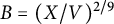 $B=(X/V)^{2/9}$
and combining (3.14) and (3.15), we obtain
 $$ \begin{align} \sum_{b\leqslant X ^{1/2}}\sum_{m\leqslant V}\min\bigg\{\dfrac{X}{b^2m}, \dfrac{1}{\|b^2m\alpha\|}\bigg\}\ll \bigg(X^{13/18}V^{5/18} + X^{1/2}V + \dfrac{X}{q^{1/4}} + X^{3/4}q^{1/4}\bigg)(\log X)^{10}. \end{align} $$
Finally, we choose
 $U=V=\min \{ X^{5/14}, q, X/q \}$
and combine (3.10), (3.11), (3.12), and (3.16) to obtain
 $$ \begin{align*} \sum_{n\leqslant X }\tilde{\mu}_2(n)\operatorname{e}(n\alpha)\ll \bigg(X^{23/28} + \dfrac{X}{q^{1/4}} + X^{3/4}q^{1/4}\bigg)(\log X)^{10}, \end{align*} $$
as it was to be shown.
4 Proof of Theorem 1.2
In order to prove Theorem 1.2, we will require the following lemma.
Lemma 4.1 Let
 $\alpha \in \mathbb {R}$
and consider a reduced fraction
 $a/q$
such that
 $|\alpha -a/q|\leqslant \gamma /q^2$
for some
 $\gamma \geqslant 1$
. Then, for
 $X \geqslant 2$
and for any fixed
 $\varepsilon>0$
, we have
 $$ \begin{align} S_{\mu}(X, \alpha) \ll_{\varepsilon} \gamma \bigg(X^{4/5+\varepsilon}+\dfrac{X(\log X)^3}{q^{1/2}} + X^{1/2}q^{1/2} (\log X)^3\bigg ), \end{align} $$
where the implied constant in (4.1) depends at most on
 $\varepsilon $
.
Proof The proof follows exactly along the lines of the proof of Theorem 1.1, except that we apply Lemmas 2.3 and 2.4 instead of Lemmas 2.1 and 2.2, respectively.
We explicitly show the proof of Theorem 1.2 in the case when
 $k=2$
. The argument then follows similarly for higher values of k using induction. We can assume
 $q \leqslant X$
; otherwise, the conclusion is trivial. We break our proof into several steps.
4.1 Initial step
Let
 $$ \begin{align*} S_{\mu_2}(X, \alpha):=\sum_{n\leqslant X }(\mu*\mu)(n)\operatorname{e}(n\alpha). \end{align*} $$
Then, for some parameters
 $2\leqslant M , N\leqslant X $
to be chosen later, we can write
 $$ \begin{align} S_{\mu_2}(X, \alpha)=&\: \sum_{\substack{mn\leqslant X \\ m> M, n>N}}\mu(m)\mu(n)\operatorname{e}(mn\alpha) + \sum_{m\leqslant M }\mu(m)\sum_{n\leqslant X /m}\mu(n)\operatorname{e}(mn\alpha)\notag \\ \notag &+\sum_{n\leqslant N}\mu(n)\sum_{m\leqslant X /n}\mu(m)\operatorname{e}(mn\alpha)-\sum_{\substack{m\leqslant M\\ n\leqslant N }}\mu(m)\mu(n)\operatorname{e}(mn\alpha)\\ =&\: S_{\mu_2}^{(1)}(X, \alpha)+S_{\mu_2}^{(2)}(X, \alpha) + S_{\mu_2}^{(3)}(X, \alpha)-S_{\mu_2}^{(4)}(X, \alpha) , \end{align} $$
say. We now turn our attention to each of these terms.
4.2 Estimation of
$S_{\mu _2}^{(1)}(X, \alpha )$
and
$S_{\mu _2}^{(4)}(X, \alpha )$
.


Applying Lemma 2.2 after the dyadic decomposition following the proof of Theorem 1.1, we deduce that
 $$ \begin{align} S_{\mu_2}^{(1)}(X, \alpha)&\ll X^{1/2}\bigg(q+\dfrac{X}{M} + \dfrac{X}{N} + \dfrac{X}{q}\bigg)^{1/2}(\log X)^2\notag\\ &\ll \bigg(X^{1/2}q^{1/2}+\dfrac{X}{M^{1/2}} + \dfrac{X}{N^{1/2}} + \dfrac{X}{q^{1/2}}\bigg)(\log X)^2. \end{align} $$
Trivially, we have
 $$ \begin{align} S_{\mu_2}^{(4)}(X, \alpha) \ll MN. \end{align} $$
4.3 Estimation of
$S_{\mu _2}^{(2)}(X, \alpha )$
and
$S_{\mu _2}^{(3)}(X, \alpha )$
.


Fix
 $\varepsilon>0$
. Writing
 $\alpha = a/q + \beta $
, one has
 $$\begin{align*}m\alpha = \dfrac{ma}{q} + m\beta = \dfrac{ma/(m, q)}{q/(m, q)} + m\beta \quad \text{and}\quad |m\beta|\leqslant\dfrac{m/(m, q)^2}{q^2/(m, q)^2} \leqslant\dfrac{m/(m, q)}{q^2/(m, q)^2}.\end{align*}$$
Therefore, using Lemma (4.1), we obtain
 $$ \begin{align} S_{\mu_2}^{(2)}(X, \alpha) & \ll_{\varepsilon} \sum_{m\leqslant M}\dfrac{m}{(m, q)}\bigg\{\bigg(\dfrac{X}{m}\bigg)^{4/5+\varepsilon} + \dfrac{X(m, q)^{1/2}(\log X)^3}{mq^{1/2}} + \bigg(\dfrac{X}{m}\bigg)^{1/2}\dfrac{q^{1/2}(\log X)^3}{(m, q)^{1/2}}\bigg \}\notag \\ &\ll_{\varepsilon} X^{4/5+\varepsilon}M^{6/5-\varepsilon} + \dfrac{XM(\log X)^3}{q^{1/2}} + X^{1/2}q^{1/2}M^{3/2}(\log X)^3. \end{align} $$
Similarly, we can show that
 $$ \begin{align} S_{\mu_2}^{(3)}(X, \alpha)\ll_{\varepsilon} X^{4/5+\varepsilon}N^{6/5-\varepsilon} + \dfrac{XN(\log X)^3}{q^{1/2}} + X^{1/2}q^{1/2}N^{3/2}(\log X)^3. \end{align} $$
4.4 Parameter optimization
Substituting the estimates (4.3), (4.5), (4.6), and (4.4) in (4.2) and choosing
 $M=N$
, we deduce that
 $$ \begin{align} S_{\mu_2}(X, \alpha) \ll_{\varepsilon} X^{4/5+\varepsilon}M^{6/5-\varepsilon}+\bigg(\dfrac{X}{M^{1/2}} + X^{1/2}q^{1/2} + \dfrac{XM}{q^{1/2}} + X^{1/2}q^{1/2}M^{3/2}\bigg)(\log X)^3. \end{align} $$
We are now left with the crucial step: to choose our parameter M optimally. Since we will choose
 $M \geqslant 1$
, we may omit the term
 $X^{1/2}q^{1/2}$
in (4.7). Let
 $M=y^5$
,
 $A= \sqrt {q}$
,
 $B = X^{1/5}$
, and
 $C = \sqrt {{X}/{q}}$
. To optimally choose M, it suffices to minimize the expression
 $$ \begin{align} H(y):= \max \bigg \{ \dfrac{1}{y^{5/2}}, \dfrac{y^5}{A}, \dfrac{y^6}{B}, \dfrac{y^{15/2}}{C} \bigg \}. \end{align} $$
Note that as a function of y, only
 $1/y^{5/2}$
is decreasing. Hence, the minimum value in (4.8) is attained when
 $1/y^{5/2}$
is equal to one of the other three functions. We consider the following cases.
Case 1. Suppose we have
 $$ \begin{align} \dfrac{y^5}{A} \geqslant \max \bigg \{ \dfrac{y^6}{B}, \dfrac{y^{15/2}}{C} \bigg \}. \end{align} $$
Then the minimum value in (4.8) is attained when
 $$\begin{align*}\frac{1}{y^{5/2}} = \frac{y^5}{A}, \end{align*}$$
which implies that
 $y = A^{2/15}$
. With this particular choice of y, we see that
 $$\begin{align*}\dfrac{y^5}{A} \geqslant \dfrac{y^6}{B} \end{align*}$$
is equivalent to
 $A^{-1/3} \geqslant A^{4/5}B^{-1}$
which occurs when
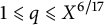 $1 \leqslant q \leqslant X^{6/17}$
. However, the inequality
 $$\begin{align*}\dfrac{y^5}{A} \geqslant \dfrac{y^{15/2}}{C} \end{align*}$$
is equivalent to
 $A^{-1/3} \geqslant AC^{-1}$
which occurs when
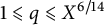 $1 \leqslant q \leqslant X^{6/14}$
. Combining the two ranges, we see that (4.9) holds when
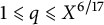 $1 \leqslant q \leqslant X^{6/17}$
. In this range, we have
 ${H(y) =A^{-1/3} = q^{-1/6}}$
, and thus,
 $$ \begin{align} S_{\mu_2}(X, \alpha) \ll \dfrac{X(\log X)^3}{q^{1/6}}. \end{align} $$
Case 2. Now let’s assume the scenario
 $$ \begin{align} \dfrac{y^6}{B} \geqslant \max \bigg \{ \dfrac{y^5}{A} , \dfrac{y^{15/2}}{C} \bigg \}. \end{align} $$
Then the minimum value in (4.8) is attained when
 $$\begin{align*}\frac{1}{y^{5/2}} = \frac{y^6}{B}, \end{align*}$$
which implies that
 $y = B^{2/17}$
. Therefore, the inequality
 $$\begin{align*}\dfrac{y^6}{B} \geqslant \dfrac{y^5}{A} \end{align*}$$
holds with
 $y=B^{2/17}$
when
 $A \geqslant B^{15/17}$
, which implies that
 $q \geqslant X^{6/17}$
. However, the inequality
 $$\begin{align*}\dfrac{y^6}{B} \geqslant \dfrac{y^{15/2}}{C} \end{align*}$$
holds with
 $y=B^{2/17}$
when
 $B \geqslant C^{17/20}$
, which implies that
 $q \leqslant X^{9/17}$
. Putting together the two ranges, we see that (4.11) holds when
 $X^{6/17}\leqslant q \leqslant X^{9/17}$
. In this range,
 ${H(y)=B^{-5/17} =X^{-1/17}}$
, and we have
 $$ \begin{align} S_{\mu_2}(X, \alpha) \ll_{\varepsilon} X^{16/17+\varepsilon}. \end{align} $$
Case 3. Arguments similar to Cases 1 and 2 show that when
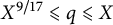 $X^{9/17}\leqslant q \leqslant X$
, then the minimum value in (4.8) is
 $H(y) = C^{-1/4}=q^{1/8}X^{-1/8} $
. Therefore in this range, we obtain
 $$ \begin{align} S_{\mu_2}(X, \alpha) \ll X^{7/8}q^{1/8}(\log X)^3. \end{align} $$
Combining the estimates (4.10), (4.12), and (4.13), we conclude that
 $$\begin{align*}\sum_{n\leqslant X }(\mu*\mu)(n)\operatorname{e}(n\alpha) \ll_{\varepsilon} X^{16/17+\varepsilon}+\bigg(\dfrac{X}{q^{1/6}} + X^{7/8}q^{1/8}\bigg)(\log X)^{3}. \end{align*}$$
This completes the proof for the case when
 $k=2$
.
4.5 Induction step
Fix
 $\varepsilon>0$
. Assume that for
 $X \geqslant 2$
,
 $$ \begin{align*} \sum_{n\leqslant X }\mu_k(n)\operatorname{e}(n\alpha) \ll_{\varepsilon} X^{a_k+\varepsilon}+ \dfrac{X(\log X)^{k^2}}{q^{b_k}} + X^{c_k}q^{1-c_k}(\log X)^{k^2}, \end{align*} $$
for some
 $k=\ell \geqslant 2$
, and we want to prove our desired result when
 $k=\ell +1$
. Similar to Lemma 4.1, one can show that if
 $\alpha \in \mathbb {R}$
such that
 $|\alpha -a/q|\leqslant \gamma /q^2$
for some
 $(a, q)=1$
and
 $\gamma \geqslant 1$
, then
 $$ \begin{align} \sum_{n\leqslant X }\mu_\ell(n)\operatorname{e}(n\alpha) \ll_{\varepsilon} \gamma \bigg(X^{a_{\ell}+\varepsilon}+ \dfrac{X(\log X)^{\ell^2}}{q^{b_{\ell}}} + X^{c_{\ell}}q^{1-c_{\ell}}(\log X)^{\ell^2} \bigg), \end{align} $$
where the implied constant in (4.14) depends at most on
 $\varepsilon $
. Equipped with (4.14), for some parameters
 $2\leqslant M, N\leqslant X$
to be chosen later, we can write
 $$ \begin{align} S_{\mu_{\ell+1}}(X, \alpha)=&\: \sum_{\substack{mn\leqslant X \\ m> M, n>N}}\mu(m)\mu_\ell (n)\operatorname{e}(mn\alpha) + \sum_{m\leqslant M}\mu(m)\sum_{n\leqslant X/m}\mu_\ell (n)\operatorname{e}(mn\alpha)\notag \\ \notag &+\sum_{n\leqslant N}\mu_\ell (n)\sum_{m\leqslant X/n}\mu(m)\operatorname{e}(mn\alpha)-\sum_{\substack{m\leqslant M\\ n\leqslant N}}\mu(m)\mu _\ell (n)\operatorname{e}(mn\alpha)\\ =&\: S_{\mu _{\ell+1} }^{(1)}(X, \alpha)+S_{\mu _{\ell+1} }^{(2)}(X, \alpha) + S_{\mu _{\ell+1} }^{(3)}(X, \alpha)-S_{\mu _{\ell+1} }^{(4)}(X, \alpha). \end{align} $$
Again, applying Lemma 2.2, we obtain
 $$ \begin{align} S_{\mu _{\ell+1} }^{(1)}(X, \alpha) \ll \bigg(X^{1/2}q^{1/2}+\dfrac{X}{M^{1/2}} + \dfrac{X}{N^{1/2}} + \dfrac{X}{q^{1/2}}\bigg)(\log X)^{(\ell+1)^2}. \end{align} $$
Trivially, we have
 $$ \begin{align} S_{\mu _{\ell+1}}^{(4)}(X, \alpha) \ll MN (\log N)^{\ell-1}. \end{align} $$
Choosing
 $\gamma = m/(m,q)$
and applying (4.14), we arrive at
 $$ \begin{align} S_{\mu _{\ell+1} }^{(2)}(X, \alpha) \ll_{\varepsilon} X^{a_\ell+\varepsilon}M^{2-a_\ell-\varepsilon}+ \dfrac{XM(\log X)^{(\ell+1)^2}}{q^{b_\ell}} + X^{c _\ell}q^{1-c _\ell}M^{2-c_\ell}(\log X)^{(\ell+1)^2}. \end{align} $$
Note that Lemma 2.7 shows that
 $$\begin{align*}\sum_{n \leqslant N } \tau_\ell^2(n) \ll N(\log N)^{\ell^2-1}.\end{align*}$$
Hence, applying Lemma (4.1) and Cauchy-Schwartz inequality in conjunction, we can write
 $$ \begin{align} S_{\mu _{\ell+1} }^{(3)}(X, \alpha) &\ll_{\varepsilon} \sum_{n \leqslant N } \tau_\ell(n) \cdot \dfrac{n}{(n, q)}\bigg\{\bigg(\dfrac{X}{n}\bigg)^{4/5+\varepsilon} + \dfrac{X(n, q)^{1/2}(\log X)^3}{nq^{1/2}} + \bigg(\dfrac{X}{n}\bigg)^{1/2}\dfrac{q^{1/2}(\log X)^3}{(n, q)^{1/2}}\bigg\} \notag \\ &\ll_{\varepsilon}X^{4/5+\varepsilon}N^{6/5-\varepsilon}+ \dfrac{XN(\log X)^{(\ell+1)^2}}{q^{1/2}} + X^{1/2}q^{1/2}N^{3/2}(\log X)^{(\ell+1)^2}. \end{align} $$
Substituting the estimates (4.16), (4.17), (4.18), and (4.19) in (4.15) and choosing
 ${M=N}$
, we have
 $$ \begin{align*} S_{\mu _{\ell+1} }(X, \alpha) \ll_{\varepsilon} X^{a _\ell+\varepsilon}M^{2-a _\ell-\varepsilon}+ \bigg(\dfrac{X}{M^{1/2}} +\dfrac{XM}{q^{b _\ell}} + X^{c _\ell}q^{1-c _\ell}M^{2-c _\ell} + X^{1/2}q^{1/2}M^{3/2}\bigg)(\log X)^{(\ell+1)^2}. \end{align*} $$
An optimization procedure similar to that for the case
 $k=2$
then shows that
 $$ \begin{align*} S_{\mu _{\ell+1} }(X, \alpha) \ll_{\varepsilon} X^{a _{\ell+1}+\varepsilon}+\dfrac{X(\log X)^{(\ell+1)^2}}{q^{b _{\ell+1}}} + X^{c _{\ell+1}}q^{1-c _{\ell+1}}(\log X)^{(\ell+1)^2}, \end{align*} $$
thereby completing the proof.
5 Proof of Theorem 1.6
We now set up the structure of the proof of Theorem 1.6. Recall from (1.9) and (1.10) that
 $$ \begin{align*} \Psi_{\mu*\mu}(z) &= \sum_{n=1}^\infty p_{\mu*\mu}(n) z^n = \prod_{n=1}^\infty (1-z^n)^{-(\mu*\mu)(n)}, \quad \lvert z \rvert <1, \\ \Phi_{\mu*\mu}(z) &= \sum_{j=1}^\infty \sum_{n=1}^\infty \frac{(\mu*\mu)(n)}{j} z^{jn}, \quad \lvert z \rvert <1, \end{align*} $$
and
 $\Psi _{\mu *\mu }(z) = \exp (\Phi _{\mu *\mu }(z))$
. The strategy to prove Theorem 1.6 is to employ the Hardy-Littlewood circle method. An application of Cauchy’s theorem yields
 $$ \begin{align} p_{\mu*\mu}(n) = \rho^{-n} \int_0^1 \exp(\Phi_{\mu*\mu}(\rho \operatorname{e}(\theta))-2\pi i n \theta) d\theta, \end{align} $$
where
 $0< \rho < 1$
. We write
 $\rho = \exp (-1/X)$
, for some parameter
 $X>0$
. As we shall see, for each value of n, we will choose
 $X = X(n)$
, and therefore,
 $\rho =\rho (n)$
in (5.1) to be such that as
 $n \to \infty $
,
 $X \to \infty $
, and
 $\rho \to 1$
. Therefore, in what follows, we can assume X to be sufficiently large. Invoking the periodicity of the integrand in (5.1), we can replace the unit interval by the interval
 $\mathcal {U} = [-X^{-1} (\log X)^A ,1-X^{-1} (\log X)^A)$
, where
 $A>0$
is a sufficiently large constant. This choice
 $\mathcal {U}$
keeps the region around the origin from being split into two regions.
Now we are ready to set up the major and minor arcs. Let
 $a \in \mathbb {N}\cup \{0\}$
and
 $q \in \mathbb {N}$
such that
 $0 \leqslant a < q$
and
 $(a,q)=1$
. Choose
 $$ \begin{align} \delta_q = q^{-1}X^{-1}(\log X)^A \quad \mathrm{and} \quad Q = (\log X)^A, \end{align} $$
and define
 $$ \begin{align} \mathfrak{M}(q,a) = \bigg\{\theta \in \mathcal{U}: \bigg|\theta-\frac{a}{q}\bigg| \leqslant \delta_q \bigg\}. \end{align} $$
The major arcs
 $\mathfrak {M}$
and the minor arcs
 $\mathfrak {m}$
are
 $$ \begin{align} \mathfrak{M} = \bigcup_{\substack{1 \leqslant a \leqslant q \leqslant Q \\ (a,q)=1}} \mathfrak{M}(q,a) \quad \mathrm{and} \quad \mathfrak{m} = \mathcal{U} \backslash \mathfrak{M}. \end{align} $$
We will show that if
 $\theta \in \mathfrak {M}$
, then
 $$ \begin{align} \Phi_{\mu * \mu}(\rho \operatorname{e} (\theta)) \ll_A \frac{X}{(\log X)^{A}}. \end{align} $$
However, if
 $\theta \in \mathfrak {m}$
, then one has
 $$ \begin{align} \Phi_{\mu * \mu}(\rho \operatorname{e} (\theta)) \ll_A \frac{X}{(\log X)^{A/9}}. \end{align} $$
Assuming for now the validity of (5.5) and (5.6), we proceed to prove Theorem 1.6.
Proof of Theorem 1.6
We rewrite (5.1) as
 $$ \begin{align} p_{\mu*\mu}(n) = \rho^{-n}\bigg(\int_{\mathfrak{M}} + \int_{\mathfrak{m}}\bigg) \exp(\Phi_{\mu*\mu}(\rho \operatorname{e} (\theta))-2\pi i n \theta) d\theta. \end{align} $$
First, we consider the integral over the minor arcs. Let
 $X = \sqrt {n} (\log n)^{A/18}$
. Since
 ${\rho =\exp (-1/X)}$
, using (5.6), we can write
 $$ \begin{align} \rho^{-n} \int_{\mathfrak{m}} \exp(\Phi_{\mu*\mu}(\rho \operatorname{e} (\theta))-2\pi i n \theta) d\theta \ll \exp \bigg(\frac{n}{X}+\frac{X}{(\log X)^{A/9}} \bigg) \ll \exp \bigg(\frac{\sqrt{n}}{(\log n)^{A/20}} \bigg). \end{align} $$
A concomitant argument holds for the major arcs. Therefore, choosing A sufficiently large, we obtain
 $$\begin{align*}\log p_{\mu*\mu}(n) \ll_B \frac{\sqrt{n}}{(\log n)^{B}}, \end{align*}$$
for any fixed
 $B>0$
.
Therefore, it suffices to establish (5.5) and (5.6), which we do in Sections 6 and 7, respectively.
6 Major arcs
We begin our discussion on the major arcs by estimating Möbius convolutions in arithmetic progressions. The key ingredient required for the following result is Lemma 2.6.
Lemma 6.1 Let
 $X \geqslant 2$
. Suppose
 $B>0$
is fixed. Let
 $r, q\geqslant 1$
be positive integers with
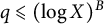 $q\leqslant (\log X)^B$
. Then there exists a constant
 $c_B>0$
depending only on B such that
 $$ \begin{align*} S(X) := \sum_{\substack{n \leqslant X \\ n \equiv r \operatorname{mod} q}} (\mu * \mu)(n) \ll_B X\exp(-c_B\sqrt{\log X}). \end{align*} $$
Proof By Dirichlet’s hyperbola method, we break
 $S(X)$
into three sub-sums; that is,
 $S(X) = S_1(X)+S_2(X) - S_3(X)$
, where
 $$ \begin{align*} S_1(X) &= \sum_{n_1 \leqslant \sqrt{X}} \mu(n_1) \sum_{\substack{n_2 \leqslant X/n_1 \\ n_1 n_2 \equiv r \operatorname{mod} q}} \mu(n_2),\\ S_2(X) &= \sum_{n_2 \leqslant \sqrt{X}} \mu(n_2) \sum_{\substack{n_1 \leqslant X/n_2 \\ n_1 n_2 \equiv r \operatorname{mod} q}} \mu(n_2),\\ S_3(X) &= \sum_{n_1 \leqslant \sqrt{X}} \mu(n_1) \notag \sum_{\substack{n_2 \leqslant \sqrt{X} \\ n_1 n_2 \equiv r \operatorname{mod} q}} \mu(n_2). \end{align*} $$
We treat
 $S_3(X)$
first. Consider the inner sum over
 $n_2$
. Note that if
 $n_1 n_2 \equiv r \operatorname {mod} q$
, then
 $n_1(n_2 + q) \equiv r \operatorname {mod} q$
. With this in mind, we write
 $$ \begin{align} \mathcal{B}:=\big\{x\operatorname{mod} q\colon n_1x \equiv r \operatorname{mod} q\big\}. \end{align} $$
Then using Lemma 2.6, it follows that
 $$ \begin{align} \sum_{\substack{n_2 \leqslant \sqrt{X} \\ n_1 n_2 \equiv r \operatorname{mod} q}} \mu(n_2) = \sum_{b \in \mathcal{B}} \sum_{\substack{n_2 \equiv b \operatorname{mod} q \\ n_2 \leqslant \sqrt{X}}} \mu(n_2) \ll_B \operatorname{card}(\mathcal{B}) \sqrt{X} \exp(-c_1 \sqrt{\log X}), \end{align} $$
for some constant
 $c_1=c_1(B)>0$
. The bound in (6.2) holds for all
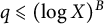 $q \leqslant (\log X)^B$
. Therefore, by trivially bounding the sum over
 $n_1$
, we obtain
 $$ \begin{align} S_3(X) \ll_B \bigg(\sum_{n_1 \leqslant \sqrt{X}} |\mu(n_1)|\bigg) \operatorname{card}(\mathcal{B}) \sqrt{X} \exp(-c_1 \sqrt{\log X}) \ll_B X \exp(-c_2 \sqrt{\log X}), \end{align} $$
for some constant
 $c_2=c_2(B)>0$
.
Note that
 $S_1(X)=S_2(X)$
by symmetry. Therefore, it is enough to estimate the sum
 $S_1(X)$
. We analyze the inner sum over
 $n_2$
first. Again applying Lemma 2.6, we obtain
 $$ \begin{align*} \sum_{\substack{n_2 \leqslant X/n_1 \\ n_1 n_2 \equiv r \operatorname{mod} q}} \mu(n_2) = \sum_{b \in \mathcal{B}} \sum_{\substack{n_2 \equiv b \operatorname{mod} q \\ n_2 \leqslant X/n_1}} \mu(n_2) \ll_B \operatorname{card}(\mathcal{B}) \frac{X}{n_1} \exp \bigg(-c_3 \sqrt{\log\frac{X}{n_1}}\bigg), \end{align*} $$
for some constant
 $c_3=c_3(B)>0$
, where
 $\mathcal {B}$
is as in (6.1). This leaves us with
 $$ \begin{align} S_1(X) &\ll_B \sum_{n_1 \leqslant \sqrt{X}} \operatorname{card}(\mathcal{B}) \frac{X}{n_1} \exp \bigg(-c_3 \sqrt{\log\frac{X}{n_1}}\bigg) \ll_B X\exp\big(-c_4\sqrt{\log X}\big), \end{align} $$
for some constant
 $c_4=c_4(B)>0$
. Combining (6.3) and (6.4), we arrive at the conclusion.
Applying Lemma 6.1, one can quickly conclude the following.
Lemma 6.2 Let
 $X \geqslant 2$
and suppose
 $B>0$
is fixed. Let
 $\theta \in \mathbb {R}$
such that
 $\theta = a/q+\beta $
, where
 $a,q \in \mathbb {Z}$
with
 $0 \leqslant a < q \leqslant (\log X)^B$
,
 $(a,q)=1$
and
 $\lvert \beta \rvert \leqslant X ^{-1}(\log X)^B$
. Then there exists a constant
 $c_B>0$
depending only on B such that
 $$ \begin{align*} \sum_{n\leqslant X }(\mu*\mu)(n)\operatorname{e}(n\theta) \ll_B X\exp(-c_B\sqrt{\log X}). \end{align*} $$
Proof By partial summation, we can write
 $$ \begin{align} \sum_{n\leqslant X }(\mu*\mu)(n)\operatorname{e}(n\theta)\ll_B (1 + |\beta|X)\max_{1\leqslant y\leqslant X }\bigg|\sum_{n\leqslant y}(\mu*\mu)(n)\operatorname{e}(na/q)\bigg|. \end{align} $$
Consequently, it is enough to estimate the sum
 $$ \begin{align} \sum_{n\leqslant y}(\mu*\mu)(n)\operatorname{e}(na/q)=\sum_{b=1}^q \operatorname{e}\bigg(\dfrac{ab}{q}\bigg)\sum_{\substack{n\leqslant y\\ n\equiv b\operatorname{mod} q}}(\mu*\mu)(n). \end{align} $$
An immediate application of Lemma 6.1 shows that for some constant
 $c_1=c_1(B)>0$
depending only on B, one has
 $$ \begin{align} \sum_{\substack{n\leqslant y\\ n \equiv b \operatorname{mod} q}}(\mu*\mu)(n)\ll_B y \exp(-c_1\sqrt{\log y}). \end{align} $$
Combining (6.5), (6.6), and (6.7), we conclude that
 $$ \begin{align*} \sum_{n\leqslant X }(\mu*\mu)(n)\operatorname{e}(n\theta)\ll_B (1+|\beta|X)qX\exp(-c_1\sqrt{\log X}) \ll_B X\exp(-c_B\sqrt{\log X}), \end{align*} $$
for some constant
 $c_B>0$
depending only on B.
Recall from (5.4) that if
 $\theta \in \mathfrak {M}$
, we can write
 $\theta =a/q+\beta $
with
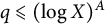 $q\leqslant (\log X)^A$
and
 $|\beta |\leqslant \delta _q \leqslant X ^{-1}(\log X)^A$
, where
 $A>0$
is sufficiently large. Using Lemmas 6.1 and 6.2, we can now prove (5.5) for
 $\theta \in \mathfrak {M}$
.
Lemma 6.3 Let
 $\theta \in \mathfrak {M}$
as defined in (5.4). Then, for any fixed
 $A>0$
,
 $$ \begin{align*} \Phi_{\mu * \mu}(\rho \operatorname{e} (\theta)) \ll_A \frac{X}{(\log X)^{A}}. \end{align*} $$
Proof Since
 $\rho = \exp (-1/X)$
, it follows from (1.10) that
 $$ \begin{align*} \Phi_{\mu * \mu}(\rho \operatorname{e}(\theta)) = \sum_{j=1}^\infty\sum_{n=1}^\infty \frac{1}{j} (\mu * \mu)(n) e^{-nj / X} \operatorname{e}(j n \theta). \end{align*} $$
We replace the exponentially damped term above by the integral
 $$ \begin{align*} e^{-nj / X} = \int_n^\infty jX^{-1}e^{-tj/X}\, dt, \end{align*} $$
leaving us with
 $$ \begin{align*} \Phi_{\mu * \mu}(\rho \operatorname{e}(\theta)) = \sum_{j=1}^\infty \frac{1}{j} \int_1^\infty jX^{-1}e^{-tj/X} \sum_{n \leqslant t} (\mu * \mu)(n) \operatorname{e}(j n \theta) \, dt. \end{align*} $$
Suppose
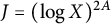 $J=(\log X)^{2A}$
. Trivially, we obtain
 $$ \begin{align} \sum_{j>J}\frac{1}{j} \int_1^\infty jX^{-1}e^{-tj/X} &\sum_{n \leqslant t} (\mu * \mu)(n) \operatorname{e}(j n \theta) \, dt \notag \\ & \ll \sum_{j>J}^\infty \frac{1}{j} \int_1^\infty jX^{-1}e^{-tj/X} t \log t \, dt \notag \\ &\ll \sum_{j>J}^\infty \frac{X \log X}{j^2} \int_{j/X}^\infty ue^{-u} \log u \, du \ll_A \frac{X}{(\log X)^{A}}. \end{align} $$
Hence, in what follows, it suffices to work with the sum
 $$ \begin{align} \sum_{j=1}^J \frac{1}{j} \int_1^\infty jX^{-1}e^{-tj/X} \sum_{n \leqslant t} (\mu * \mu)(n) \operatorname{e}(j n \theta) \, dt. \end{align} $$
Writing
 $\theta =a/q+\beta $
with
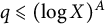 $q\leqslant (\log X)^A$
and
 $|\beta |\leqslant \delta _q \leqslant X ^{-1}(\log X)^A$
, one has
 $$\begin{align*}\theta _j := j\theta = \frac{aj/(j,q)}{q/(j,q)}+ j\beta = \frac{a _j}{q _j}+\beta _j, \end{align*}$$
where
 $(a _j,q _j)=1$
,
 $1 \leqslant q _j \leqslant q \leqslant (\log X)^{A} $
and
 $\beta _j \leqslant X ^{-1}(\log X)^{3A}$
. We can now break the inner integral in (6.9) as
 $$ \begin{align*} I &= \int_1^\infty jX^{-1}e^{-tj/X} \sum_{n \leqslant t} (\mu * \mu)(n) \operatorname{e}(j n \theta) \, dt \\ &= \bigg(\int_1^{X \log X} + \int_{X\log X}^\infty\bigg) jX^{-1}e^{-tj/X} \sum_{n \leqslant t} (\mu * \mu)(n) \operatorname{e}(j n \theta) \, dt = I_1+I_2, \end{align*} $$
say. For
 $I_2$
, one has
 $$ \begin{align} I_2 & \ll \int_{X\log X}^\infty jX^{-1}e^{-tj/X} t \log t \, dt \ll \frac{X \log X}{j} \int_{\log X}^\infty ue^{-u} \log u \, du \ll_A \frac{X}{(\log X)^{3A}}. \end{align} $$
For
 $I_1$
, an application of Lemma 6.2 shows that
 $$ \begin{align} I_1 & \ll_A X \log X \exp(-C_A \sqrt{\log X}) \int_1^{X\log X} jX^{-1}e^{-tj/X} \, dt \notag \\ & \ll_A X \log X \exp(-C_A \sqrt{\log X}) \int_{1}^{X\log X} e^{-u} \, du \ll_A \frac{X}{(\log X)^{3A}}, \end{align} $$
where
 $C_A>0$
is a constant depending only on A. Putting together (6.10) and (6.11), we obtain
 $$\begin{align*}\sum_{j=1}^J \frac{1}{j} \int_1^\infty jX^{-1}e^{-tj/X} \sum_{n \leqslant t} (\mu * \mu)(n) \operatorname{e}(j n \theta) \, dt \ll_A \frac{X}{(\log X)^{A}}. \end{align*}$$
Combining this with (6.8), we arrive at our desired conclusion.

7 Minor Arcs
In general, being able to show that the contribution of the minor arcs is of lower order than the principal arcs is the most challenging aspect of successfully deploying the circle method. In situations such as [Reference Berndt, Malik and Zaharescu2, Reference Gafni11], which involved partitioning with respect to powers or powers in arithmetic progressions, one requires Weyl’s inequality [Reference Vaughan31, Lemma 2.4] in conjunction with Hua’s inequality [Reference Vaughan31, Theorem 4.1]. Adapting Weyl’s inequality was also a key aspect for partitioning with respect to polynomials in [Reference Dunn and Robles10]. Restricted partitions with respect to primes [Reference Vaughan32] necessitated Vinogradov’s inequality [Reference Vaughan31, Chapter 3]. However, Vinogradov’s inequality was not sufficient for functions of primes. In [Reference Gafni12], Gafni employed a bound by Kawada and Wooley [Reference Kawada and Wooley15], and in [Reference Das, Robles, Zaharescu and Zeindler8], a new bound altogether for exponential sums dealing with semiprimes was introduced and proved. This was also the case in [Reference Berndt, Robles, Zaharescu and Zeindler3, §6] where a bound for exponential sums twisted by generalized divisor functions had to be supplied. In our current situation, the exponential sums discussed in Section 1 and proved in Sections 3 and 4 will serve as the main technology to bound the contributions from the minor arcs. It is worth remarking that interesting exponential sums for minor arcs can also be found in [Reference Kumchev20].
We begin by recording the immediate corollary from Theorem 1.2 for the case when
 $k=2$
.
Corollary 7.1 Let
 $\alpha \in \mathbb {R}$
and consider a reduced fraction
 $a/q$
such that
 $|\alpha -a/q|\leqslant 1/q^2$
. Then, for
 $X \geqslant 2$
and any fixed
 $\varepsilon>0$
, we have
 $$ \begin{align*} \sum_{n\leqslant X }(\mu*\mu)(n)\operatorname{e}(n\alpha) \ll_{\varepsilon} X^{16/17+\varepsilon}+\bigg(\dfrac{X}{q^{1/6}} + X^{7/8}q^{1/8}\bigg)(\log X)^{3}. \end{align*} $$
Now we are ready to prove (5.6) for
 $\theta \in \mathfrak {m}$
.
Lemma 7.2 Let
 $\theta \in \mathfrak {m}$
as defined in (5.4). Then, for any fixed
 $A>0$
,
 $$ \begin{align*} \Phi_{\mu * \mu}(\rho \operatorname{e} (\theta)) \ll_A \frac{X}{(\log X)^{A/9}}. \end{align*} $$
Proof As in the proof of Lemma 6.3, it suffices to only consider the sum
 $$\begin{align*}\sum_{j=1}^J \frac{1}{j} \int_1^\infty jX^{-1}e^{-tj/X} \sum_{n \leqslant t} (\mu * \mu)(n) \operatorname{e}(j n \theta) \, dt, \end{align*}$$
where
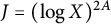 $J=(\log X)^{2A}$
. For each
 $j \leqslant J$
, we employ Dirichlet’s theorem (see [Reference Vaughan31, Lemma 2.1]) to choose
 $a \in \mathbb {Z}$
and
 $q \in \mathbb {N}$
with
 $(a,q)=1$
such that
 $$ \begin{align*} \bigg| j \theta - \frac{a}{q} \bigg| \leqslant q^{-1} X^{-1} (\log X)^A \quad \mathrm{and} \quad q < X(\log X)^{-A}. \end{align*} $$
We now set
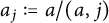 $a _j:= a/(a,j)$
and
 $q _j:=jq/(a,j)$
. The definition of
 $\delta _q$
in (5.2) implies that
 $$ \begin{align*} \bigg| \alpha - \frac{a _j}{q _j} \bigg| \leqslant \delta_{q _j}. \end{align*} $$
Since
 $\alpha \in \mathfrak {m}$
, it follows that
 $q _j> Q$
, where
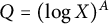 $Q=(\log X)^A$
. Now, applying Corollary 7.1, we obtain
 $$ \begin{align} \sum_{n \leqslant t} (\mu * \mu)(n) \operatorname{e}(j n \theta) \ll_{\varepsilon} t^{16/17+\varepsilon}+\dfrac{t(\log t)^{3}}{q^{1/6}} + t^{7/8}q^{1/8}(\log t)^{3}. \end{align} $$
Integrating each of the three terms on the right-hand side of (7.1) yields
 $$ \begin{align*} E_1(X,j) &= \int_1^\infty t^{16/17+\varepsilon} j X^{-1} e^{-tj/X} \, dt \ll_{\varepsilon} \bigg(\frac{X}{j}\bigg)^{16/17+\varepsilon}, \\ E_2(X,j) &= \int_1^\infty \frac{t}{q^{1/6}} (\log t)^3 j X^{-1} e^{-tj/X} \, dt \ll \frac{X}{{j{q^{1/6}}}}\left( {\log X} \right)^3, \\ E_3(X,j) &= \int_1^\infty t^{\frac{7}{8}}q^{\frac{1}{8}} (\log t)^{3} j X^{-1} e^{-tj/X} \, dt \ll {\left( {\frac{X}{j}} \right)^{\frac{7}{8}}}{q^{1/8}}\left( {\log X} \right)^3. \end{align*} $$
Note that
 $jq \geqslant q _j> (\log X)^{A}$
, and by our choice,
 $ q < X(\log X)^{-A} $
. Therefore, we conclude that
 $$ \begin{align*} \sum_{j=1}^J \frac{1}{j} \int_1^\infty jX^{-1}e^{-tj/X} \sum_{n \leqslant t} (\mu * \mu)(n) \operatorname{e}(j n \theta) \, dt \ll \sum_{j=1}^J \frac{1}{j} (E_1+E_2+E_3) \ll \frac{X}{(\log X)^{A/9}}, \end{align*} $$
which is the bound that we wanted to show.

8 Proof of Theorem 1.7
In order to prove Theorem 1.7, we need to investigate how
 $\Phi _{\mu *\mu }(z)$
behaves in the major arc and examine the effect that the nontrivial zeros of the Riemann zeta-function have on its behavior. We break our proof into several steps.
Initial setup
Recall that
 $$ \begin{align} \Phi_{\mu * \mu}(\rho \operatorname{e}(\theta)) = \sum_{j=1}^\infty \sum_{n=1}^\infty \frac{(\mu * \mu)(n)}{j} \exp\bigg( -jn \bigg(\frac{1}{X}-2\pi i \theta\bigg)\bigg), \end{align} $$
where
 $\rho =\exp (-1/X)$
. We first apply the Cahen-Mellin formula and rewrite (8.1) to obtain
 $$ \begin{align*} \Phi_{\mu * \mu}(\rho \operatorname{e}(\theta)) = \sum_{j=1}^\infty \sum_{n=1}^\infty \frac{(\mu * \mu)(n)}{j} \frac{1}{2 \pi i} \int_{(c)} \Gamma(s) j^{-s} n^{-s} \bigg(\frac{X}{1-2\pi i X \theta}\bigg)^s ds, \end{align*} $$
for
 $c>0$
. Interchanging the summations and the integration, for any real
 $c>1$
, we have
 $$ \begin{align} \Phi_{\mu * \mu}(\rho \operatorname{e}(\theta)) &= \frac{1}{2 \pi i} \int_{(c)} \Gamma(s) \bigg(\sum_{j=1}^\infty \frac{1}{j^{s+1}}\bigg) \bigg(\sum_{n=1}^\infty \frac{(\mu * \mu)(n)}{n^s} \bigg) \bigg(\frac{X}{1-2\pi i X \theta}\bigg)^s ds \nonumber \\ &= \frac{1}{2 \pi i} \int_{(c)} \Gamma(s) \zeta(s+1) \frac{1}{\zeta^2(s)} \bigg(\frac{X}{1-2\pi i X \theta}\bigg)^s ds. \end{align} $$
Contour shifting.
The path of integration in 8.2 is a vertical line with
 $\operatorname {Re}(s)=c>1$
. We move the portion
 $|t| \leqslant T$
of this path to the left, replacing it by a rectangular path joining the points
 $c \pm i T$
and
 $-u \pm i T$
, where
 $u=2N+1$
, for some large
 $N \in \mathbb {N}$
. Thus, the new path of integration is of the form
 $L=\bigcup _{i=1}^5 L_i$
, with
 $L_1=(c-i \infty , c-i T], L_2=[c-i T, -u-i T], L_3=[-u-i T, -u+i T], L_4=[-u+i T, c+i T]$
and
 $ L_5=[c+i T, c+i \infty )$
. With this change of the path of integration, an application of the Cauchy residue theorem shows that
 $$\begin{align*}\Phi_{\mu * \mu}(\rho \operatorname{e}(\theta)) = M+\frac{1}{2 \pi i} \sum_{j=1}^5 I_j, \end{align*}$$
where M denotes the contribution of the residues at singularities of the integrand in the region enclosed by the two paths and
 $I_j$
denotes the integral over the path
 $L_j$
. Our method will require an analysis of the
 $I_j$
’s. Equipped with Lemma 2.8, we will establish our results unconditionally. For similar techniques, the reader is referred to the works of Bartz [Reference Bartz1], Ramachandra and Sankaranarayanan [Reference Ramachandra and Sankaranarayanan25], and Inoue [Reference Inoue14].
Residue computations
Set
 $$\begin{align*}y:=\frac{X}{1-2\pi i X\theta}. \end{align*}$$
A singularity analysis regarding the integrand in (8.2) shows the following. We have a double pole at
 $s=0$
coming from
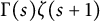 $\Gamma (s)\zeta (s+1)$
for which
 $$ \begin{align*} \mathop{\operatorname{res}}\limits_{s=0} \Gamma(s) \zeta(s+1) \frac{1}{\zeta^2(s)} y^s = 4 \log y - 8 \log(2 \pi). \end{align*} $$
The simple pole at
 $s=-1$
yields
 $$ \begin{align*} \mathop{\operatorname{res}}\limits_{s=-1} \Gamma(s) \zeta(s+1) \frac{1}{\zeta^2(s)} y^s = - \frac{\zeta(0)}{\zeta^2(-1)y} = \frac{72}{y}. \end{align*} $$
Unlike previous cases in the literature [Reference Berndt, Malik and Zaharescu2, Reference Berndt, Robles, Zaharescu and Zeindler3, Reference Das, Robles, Zaharescu and Zeindler8, Reference Dunn and Robles10, Reference Gafni11, Reference Gafni12], we now capture residues from the trivial and nontrivial zeros of the Riemann zeta-function. We start with the nontrivial zeros. Those take place at
 $s = \varpi $
and yield double poles for which
 $$ \begin{align*} \mathop{\operatorname{res}}\limits_{s=\varpi} \Gamma(s) \zeta(s+1) \frac{1}{\zeta^2(s)} y^s &= y^{\varpi} \Gamma(\varpi) \frac{\zeta(1+\varpi)}{\zeta'(\varpi)^2}\bigg(\log y + \psi(\varpi) - \frac{\zeta"}{\zeta'}(\varpi) + \frac{\zeta'}{\zeta}(1+\varpi) \bigg), \end{align*} $$
where we have used the simplicity of the zeros to alleviate the notation. For the trivial zeros, we have triple poles at
 $s=-2n$
, for
 $n=1,2,3,\dots $
, coming from
 $\Gamma (s)/\zeta ^2(s)$
. These residues can be written as
 $$ \begin{align*} \mathop{\operatorname{res}}\limits_{s=-2n} \Gamma(s) \zeta(s+1) \frac{1}{\zeta^2(s)} y^s = y^{-2 n}(\mathfrak{c}_1(n)(\log y)^2 + \mathfrak{c}_2(n)\log y + \mathfrak{c}_3(n)), \end{align*} $$
where the coefficients are given by
 $$ \begin{align} \mathfrak{c}_1(n) &:= -\frac{B_{2 n}}{8 n^2 \Gamma (2 n) \zeta '(-2 n)^2},\end{align} $$
 $$ \begin{align} \mathfrak{c}_2(n) &:= \frac{B_{2 n} \zeta "(-2 n)+\zeta '(-2 n) \left(2 n \zeta '(1-2 n)-B_{2 n} \psi (2n+1)\right)}{2 n (2 n)! \zeta '(-2 n)^3}, \end{align} $$
and
 $$ \begin{align} \mathfrak{c}_3(n) &:= \frac{1}{48 n^2 \Gamma (2 n) \zeta '(-2 n)^4} \nonumber \\&\quad \times \big[ B_{2 n} \big\{-9 \zeta "(-2 n)^2-2 \left(3 \psi(2 n+1)^2-3 \psi'(2 n+1)+\pi ^2\right) \zeta '(-2 n)^2 \nonumber \\ &\quad \quad +4 \zeta '(-2 n) (\zeta "'(-2 n)+3 \psi(2 n+1) \zeta "(-2 n))\big\} \nonumber \\ &\quad \quad +12 n \zeta '(-2 n) \left(\zeta '(-2 n) \zeta "(1-2 n)+2 \zeta '(1-2 n) \left(\psi(2 n+1) \zeta '(-2 n)-\zeta "(-2 n)\right)\right) \kern-1pt\big].\nonumber\\ \end{align} $$
Here,
 $\psi (x) = \Gamma '/\Gamma (x)$
denotes the digamma function and
 $B_n$
denotes the Bernoulli numbers.
Estimating the vertical integral
$I_3$

Using Stirling’s formula, for
 $\operatorname {Re}(s) \leqslant -3/2$
,
 $$ \begin{align} \Gamma(s)\zeta(s+1)\zeta(s) \ll (2 \pi)^{2\operatorname{Re}(s)}\lvert s \rvert^{-\operatorname{Re}(s)-1/2} e^{-\pi \lvert t \rvert/2}. \end{align} $$
Therefore, we have
 $$ \begin{align} I_3 = \int_{-u-iT}^{-u+iT} \Gamma(s)\zeta(s+1)\frac{1}{\zeta^2(s)}y^s \,ds &\ll \int_{-u-iT}^{-u+iT} \frac{(2 \pi)^{-2u}\lvert s \rvert^{u-1/2} e^{-\pi \lvert t \rvert/2}}{\zeta^3(s)}y^s \,ds \notag \\ &\ll \frac{1}{(2\pi)^{2u}} \int_{-u-iT}^{-u+iT} \frac{(u^2+\lvert t \rvert^2 )^{u/2-1/4} e^{-\pi \lvert t \rvert/2}}{\zeta^3(s)}y^s \,ds. \end{align} $$
We apply the functional equation for
 $\zeta (s)$
in (8.7) alongside the observation that
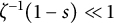 $\zeta ^{-1}(1-s) \ll 1$
. Also, following [Reference Vaughan33] (See Lemma 2.8),
 $$\begin{align*}\lvert y \rvert^s \leqslant(X\Delta)^{-u}e^{-\lvert t \rvert(\Delta-\pi/2)}.\end{align*}$$
Hence, we obtain
 $$ \begin{align} I_3 &\ll \frac{2^{3u} \pi^{3(u-1)}}{(2\pi)^{2u} (X \Delta)^{u}} \int_{-u-iT}^{-u+iT} \frac{(u^2+\lvert t \rvert^2 )^{u/2-1/4} e^{-\lvert t \rvert \Delta}}{\sin^3(\pi s/2)\Gamma^3(1-s)} \,ds. \end{align} $$
Next, we note that in our range of integration,
 $$ \begin{align*} \frac{1}{\Gamma(1-s)} \ll e^{(u+1) - (u+\frac{1}{2})\log (u+1) + \frac{1}{2}\pi |t|} \quad \mathrm{and} \quad \frac{1}{\sin(\pi s/2)} \ll e^{- \frac{1}{2}\pi |t|}. \end{align*} $$
Inserting these two bounds in (8.8), we arrive at
 $$ \begin{align} I_3 &\ll \frac{(2\pi)^{u}e^{3(u+1) - 3(u+\frac{1}{2})\log (u+1)}}{ (X \Delta)^{u}} \int_{-T}^{T} (u^2+\lvert t \rvert^2 )^{u/2-1/4} e^{-\lvert t \rvert \Delta} \,dt, \notag \\ &\ll \frac{(2\pi)^{u}e^{3(u+1) - 3(u+\frac{1}{2})\log (u+1)}}{ (X \Delta)^{u}} \int_{0}^{T} (u^2+t^2 )^{u/2-1/4} e^{-t \Delta} \,dt. \end{align} $$
We consider the inside integral in (8.9). We divide this into two cases. When
 $t \leqslant u$
, we have
 $$ \begin{align} \int_{0}^{T} (u^2+t^2 )^{u/2-1/4} e^{-t \Delta} \,dt \ll 2^{u/2}u^{u-1/2} \int_{0}^{\infty} e^{-t \Delta} \,dt \ll 2^{u/2}u^{u-1/2} \Delta^{-1}. \end{align} $$
However, when
 $t>u$
,
 $$ \begin{align} \int_{0}^{T} (u^2+t^2 )^{u/2-1/4} e^{-t \Delta} \,dt \ll 2^{u/2} \int_{0}^{\infty} t^{u-1/2} e^{-t \Delta} \,dt \ll 2^{u/2}\Gamma(u+1/2)\Delta^{-u-1/2}. \end{align} $$
Therefore, applying (8.10) and (8.11) in (8.9) and using Stirling’s approximation for
 $\Gamma (u+1/2)$
, we obtain
 $$ \begin{align} I_3 &\ll \frac{(2\sqrt{2}\pi)^{u}e^{3(u+1) - 3(u+\frac{1}{2})\log (u+1)}}{ (X \Delta)^{u}} (u^{u-1/2} \Delta^{-1}+ \Gamma(u+1/2)\Delta^{-u-1/2})\notag \\ &\ll \bigg (\frac{2\sqrt{2}\pi e^2}{X\Delta^2} \bigg)^{u}( u^{-2u-3/2} \Delta^{-1/2}). \end{align} $$
Estimating the horizontal integrals
$I_2$
and
$I_4$
.


We consider
 $I_4$
only. The treatment for
 $I_2$
is similar. Dividing the contour into two parts, we write
 $$\begin{align*}I_4 = \int_{-u+iT}^{-3/2+iT}+ \int_{-3/2+iT}^{c+iT} = I_{4,1}+I_{4,2}, \end{align*}$$
say. We work with
 $I_{4,1}$
first. Applying (8.6), we have
 $$ \begin{align} I_{4,1} = \int_{-u+iT}^{-3/2+iT} \Gamma(s) \zeta(s+1) \frac{1}{\zeta^2(s)} y^s \,ds &\ll \int_{-u+iT}^{-3/2+iT} \frac{(2 \pi)^{2\sigma}\lvert s \rvert^{-\sigma-1/2} e^{-\pi T/2}}{\zeta^3(s)}y^s \,ds \notag \\ &\ll e^{-\pi T/2} \int_{-u+iT}^{-3/2+iT} \frac{(2\pi)^{2\sigma}(\sigma^2+T^2 )^{-\sigma/2-1/4}}{ \zeta^3(s)}y^s \,ds. \end{align} $$
Proceeding as in the case of
 $I_3$
, we apply the functional equation for
 $\zeta (s)$
in (8.13) to obtain
 $$ \begin{align*} I_{4,1} &\ll e^{-T\Delta} \int_{-u+iT}^{-3/2+iT} \frac{(2\pi)^{2\sigma} (X\Delta)^\sigma (\sigma^2+T^2 )^{-\sigma/2-1/4}}{2^{3\sigma} \pi^{3(\sigma-1)}\sin^3(\pi s/2)\Gamma^3(1-s)} \,ds. \end{align*} $$
In our range of integration,
 $$ \begin{align*} \frac{1}{\Gamma(1-s)} \ll e^{1-\sigma - (\frac{1}{2}-\sigma)\log (1-\sigma) + \frac{1}{2}\pi T} \quad \mathrm{as\ well\ as} \quad \frac{1}{\sin(\pi s/2)} \ll e^{- \frac{1}{2}\pi T}. \end{align*} $$
Therefore, we arrive at
 $$ \begin{align} I_{4,1} &\ll e^{-T\Delta} \int_{-u}^{-3/2} (2\pi)^{-\sigma}(X\Delta)^\sigma (\sigma^2+T^2 )^{-\sigma/2-1/4}e^{3(1-\sigma) - 3(\frac{1}{2}-\sigma)\log (1-\sigma)} \,d\sigma \notag \\ &\ll e^{-T\Delta} \int_{3/2}^{u} \bigg (\frac{2\pi e^3}{X\Delta} \bigg)^{\sigma} \frac{(\sigma^2+T^2 )^{\sigma/2-1/4}}{ (\sigma+1)^{3(\sigma+\frac{1}{2})}} \,d\sigma. \end{align} $$
We write (8.14) as
 $$\begin{align*}e^{-T\Delta}\int_{3/2}^{u} \bigg (\frac{2\pi e^3}{X\Delta} \bigg)^{\sigma} \frac{(\sigma^2+T^2 )^{\sigma/2-1/4}}{ (\sigma+1)^{3(\sigma+\frac{1}{2})}} \,d\sigma = e^{-T\Delta}\int_{3/2}^{T}+ e^{-T\Delta}\int_{T}^{u} = J_1 +J_2, \end{align*}$$
say. Consider
 $J_1$
first. We have
 $$\begin{align*}J_1 \ll e^{-T\Delta}\int_{3/2}^{T} \bigg (\frac{2\sqrt{2}\pi e^3 T}{\sigma^3} \bigg)^{\sigma} \,d\sigma. \end{align*}$$
Let f be defined as
 $$\begin{align*}f(\sigma) = \bigg (\frac{2\sqrt{2}\pi e^3 T}{\sigma^3} \bigg)^{\sigma}, \end{align*}$$
and suppose
 $g(\sigma ) = \log f(\sigma )$
. The maximum of
 $g(\sigma )$
is attained at
 $\sigma _{0} = (2\sqrt {2}\pi T )^{1/3}$
. Hence, the maximum value attained by f in our range of integration is
 $\exp (3(2\sqrt {2}\pi T )^{1/3})$
. Therefore, we have
 $$ \begin{align} J_1 \ll e^{-T\Delta} e^{3(2\sqrt{2}\pi T )^{1/3}} T \ll e^{-T\Delta/2}. \end{align} $$
For
 $J_2$
, we obtain
 $$ \begin{align} e^{-T\Delta}\int_{T}^{u} \bigg (\frac{2\pi e^3}{X\Delta} \bigg)^{\sigma} \frac{(\sigma^2+T^2 )^{\sigma/2-1/4}}{ (\sigma+1)^{3(\sigma+\frac{1}{2})}} \,d\sigma \ll e^{-T\Delta}\int_{T}^{u} \bigg (\frac{2\sqrt{2}\pi e^3}{\sigma^2} \bigg)^{\sigma} \,d\sigma \ll e^{-T\Delta/2}. \end{align} $$
Now, we consider
 $I_{4,2}$
, which is given by
 $$ \begin{align*} I_{4,2} = \int_{-3/2+iT}^{c+iT} \Gamma(s) \zeta(s+1) \frac{1}{\zeta^2(s)} y^s \,ds. \end{align*} $$
In our range of integration,
 $$ \begin{align} \Gamma(s) \ll T^{\sigma-1/2}e^{-\pi T/2}, \quad \textrm{and} \quad \zeta(s+1) \ll T^\eta, \end{align} $$
for some fixed constant
 $\eta>0$
. We write
 $$\begin{align*}I_{4,2} = \bigg(\int_{-3/2+iT}^{-1+iT} +\int_{-1+iT}^{c+iT}\bigg) \Gamma(s) \zeta(s+1) \frac{1}{\zeta^2(s)} y^s \,ds. \end{align*}$$
For the first part, we apply the functional equation for
 $\zeta (s)$
to obtain
 $$ \begin{align} \int_{-3/2+iT}^{-1+iT} \Gamma(s) \zeta(s+1) \frac{1}{\zeta^2(s)} y^s \,ds &\ll \frac{T^{\eta-1/2}}{e^{T\Delta}}\int_{-3/2}^{-1} \bigg(\frac{X\Delta T}{2\pi e}\bigg)^{\sigma}\frac{1}{(1-\sigma)^{1/2-\sigma}} \,d\sigma \notag\\ &\ll \frac{T^{\eta-1/2}}{e^{ T\Delta}}\int_{1}^{3/2} \bigg(\frac{2\pi e}{X\Delta T}\bigg)^{\sigma}\frac{1}{(1+\sigma)^{1/2+\sigma}} \,d\sigma \ll e^{- T\Delta /2}. \end{align} $$
For the second part, using Lemma 2.8, for
 $-1 \leqslant \operatorname {Re}(s)=\sigma \leqslant 2$
and any
 $\epsilon>0$
, for sufficiently large
 $V>0$
, there exists some
 $V \leqslant T_{*} \leqslant 2V$
such that
 $$ \begin{align} \frac{1}{\zeta^2(\sigma+iT_{*})}\ll T_{*}^{\epsilon}. \end{align} $$
Therefore, using the bounds (8.17) and (8.19) and choosing
 $T=T_{*}$
, we arrive at
 $$ \begin{align} \int_{-1+iT}^{c+iT} \Gamma(s) \zeta(s+1) \frac{1}{\zeta^2(s)} y^s \,ds &\ll \frac{T^{-1/2+\eta+\epsilon}}{e^{T\Delta}}\int_{-1}^{c} (X\Delta T)^{\sigma} \,d\sigma \ll e^{- T\Delta /2}. \end{align} $$
Finally, combining the estimates (8.15), (8.16), (8.18), and (8.20), we conclude that
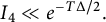 ${I_4 \ll e^{- T\Delta /2}.}$
Estimating the vertical integrals
$I_1$
and
$I_5$
.


Writing
 $$\begin{align*}I_1 = \int_{c+iT}^{c+i\infty} \Gamma(s) \zeta(s+1) \frac{1}{\zeta^2(s)} y^s \,ds, \end{align*}$$
we note that in our range of integration,
 $$ \begin{align*} \Gamma(s) &\ll e^{-\pi T/2}, \quad \zeta(s+1) \ll 1, \quad \zeta^{-2}(s) \ll 1, \quad \textrm{and} \quad \lvert y \rvert^s \leqslant(X\Delta)^{\sigma}e^{-T(\Delta-\pi/2)}. \end{align*} $$
Combining these estimates, we obtain
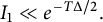 $I_1 \ll e^{- T\Delta /2}.$
A similar argument holds true for
 $I_5$
.
Final steps
Combining the estimates from the integrals and letting
 $N \to \infty $
, we obtain
 $$ \begin{align} \Phi_{\mu * \mu}(\rho \operatorname{e}(\theta)) &= 4 \log \frac{X}{1-2\pi i X\theta} - 8 \log(2 \pi) + 72 \frac{1-2\pi i X\theta}{X}\nonumber \\ & \quad +\sum_{|\operatorname{Im}(\varpi)| < T_\nu} f(X,\theta,\varpi) +\sum_{n=1}^{\infty} g(X,\theta,n) +O(e^{- T_\nu\Delta /2}), \end{align} $$
where
 $\nu \leqslant T_\nu \leqslant 2\nu$
,
 $\nu \in \mathbb {N}$
, the sum over
 $\varpi $
runs along all the nontrivial zeros of
 $\zeta $
, and
 $f,g$
are as defined in the statement of the theorem. Finally, we let
 $ \nu \to \infty $
and choose our sequence of
 $T_{\nu }$
appropriately such that (8.19) is satisfied. We conclude that
 $$ \begin{align*} \Phi_{\mu * \mu}(\rho \operatorname{e}(\theta)) &= 4 \log \frac{X}{1-2\pi i X\theta} - 8 \log(2 \pi) + 72 \frac{1-2\pi i X\theta}{X}\nonumber \\ & \quad + \lim_{\nu \to \infty} \sum_{|\operatorname{Im}(\varpi)| < T_\nu} f(X,\theta,\varpi) +\sum_{n=1}^{\infty} g(X,\theta,n), \end{align*} $$
thereby finishing the last step of the proof.
Acknowledgements
We thank Kunjakanan Nath for many comments and discussions on the subject of the paper. We also thank Dorian Goldfeld for useful suggestions. The authors are grateful to the referees for making valuable suggestions that have greatly increased the clarity and value of the manuscript. Lastly, NR wishes to acknowledge support from Vikram Kilambi and from Christopher Pernin.