




No CrossRef data available.
COMBINING FORECASTING PROCEDURES: SOME THEORETICAL RESULTS
Published online by Cambridge University Press: 05 March 2004
Abstract
We study some methods of combining procedures for forecasting a continuous random variable. Statistical risk bounds under the square error loss are obtained under distributional assumptions on the future given the current outside information and the past observations. The risk bounds show that the combined forecast automatically achieves the best performance among the candidate procedures up to a constant factor and an additive penalty term. In terms of the rate of convergence, the combined forecast performs as well as if the best candidate forecasting procedure were known in advance.
Empirical studies suggest that combining procedures can sometimes improve forecasting accuracy over the original procedures. Risk bounds are derived to theoretically quantify the potential gain and price of linearly combining forecasts for improvement. The result supports the empirical finding that it is not automatically a good idea to combine forecasts. Indiscriminate combining can degrade performance dramatically as a result of the large variability in estimating the best combining weights. An automated combining method is shown in theory to achieve a balance between the potential gain and the complexity penalty (the price of combining), to take advantage (if any) of sparse combining, and to maintain the best performance (in rate) among the candidate forecasting procedures if linear or sparse combining does not help.This research was supported by U.S. National Security Agency Grant MDA9049910060 and U.S. National Science Foundation CAREER Grant DMS0094323. The author sincerely thanks three reviewers and Poti Giannakouros for their very valuable comments, which led to a substantial improvement of the paper.
Information
- Type
- Research Article
- Information
- Copyright
- © 2004 Cambridge University Press
1. INTRODUCTION
Forecasting or prediction is of interest in many scientific fields. Depending on the nature of the process of constructing forecasts, model-based methods or more subjective opinion-based methods are used. Model-based methods include empirically based modeling, utilizing statistical tools and theory-based modeling, which depends mainly on theories from the subject field. Opinion-based methods require extensive experience in the subject field. Usually, experts' predictions are based on a difficult-to-quantify mixture of many different sources of information (qualitative and/or quantitative) and their subjective intuition or beliefs. Research in various fields has strongly suggested that the performance of prediction can be enhanced when (sometimes even in simple fashion) forecasts are combined. A survey of research results on combining forecasts is in Clemen (1989).
Although the idea of combining models/wisdom is attractive, the challenge, of course, is how to do it right. Although many approaches have been proposed for combining forecasts, with much empirical evidence of success and some theoretical justification, there is still a lack of general theoretical understanding. A difficulty is that the forecasts to be combined can be completely different in their derivations and assumptions, and therefore the commonly used methods for comparing statistical models such as model selection criteria or the traditional hypothesis testing techniques are not generally applicable. As pointed out by, e.g., Armstrong (1989) and others, the research in the area of combining forecasts so far provides few guidelines for applications.
In this paper, we propose some methods for combining point forecasts of a continuous variable and address several issues on combining forecasts. We focus on theoretical developments.
1.1. Setup of the Problem
Suppose that we are interested in forecasting or predicting a real-valued continuous random variable Y. Let Y1, Y2,… be the true values at time 1, 2,…, respectively. At each time i ≥ 1 (possibly) related qualitative and/or quantitative information, denoted jointly by Xi (which thus could be multidimensional) is observed prior to the occurrence of Yi. We need to predict Yi based on Xi and the earlier data Zi−1 = (Xl,Yl)l=1i−1. After Yi is revealed, a possible discrepancy (loss) occurs between the forecast and the true value Yi. The goal of forecasting is to make the discrepancy as small as possible.
Assume that for i ≥ 1, the conditional distribution of Yi given Xi = xi and Zi−1 = zi−1 has (conditional) mean mi and variance vi. That is, Yi = mi + ei, where ei is the random error representing the conditional uncertainty in Y at time i. The conditional mean and variance mi and vi depend on xi and zi−1 in general. Note that E(ei|Xi, Zi−1) = 0 almost surely for i ≥ 1. Let

be a predicted value of Yi. Then

where Ei denotes the conditional expectation given Zi−1 = zi−1 and Xi = xi. The decomposition indicates that given zi−1 and xi, the expected total square error of

has two components: the squared difference (bias) between

and the unknown conditional mean mi, and the conditional uncertainty vi. The latter cannot be controlled and therefore is always present regardless of which method is used for prediction. The best we can hope for is that

equals (or is very close to) mi. Because vi is the same for all forecasts, it will not be included in our measure of performance. Accordingly, we may consider the loss function

Let δ be a forecasting procedure yielding forecasts

at times 1, 2, and so on. We consider the average risk in prediction up to the present time n, denoted by R(δ; n), as the performance measure of the forecasting method δ, i.e.,

where the expectation is taken with respect to the randomness of Zn−1 and Xn.
Now suppose we have a collection of forecasting procedures, denoted by Δ = {δ1, δ2,…}. The number of forecasting procedures in Δ can be large or even countably infinite. This, from a theoretical point of view, is appropriate to study because it captures the complexity when the number of candidate forecasting procedures is large relative to n. For each forecasting procedure δj ∈ Δ, at each time i ≥ 1, the procedure gives a predicted value or forecast

based on zi−1 and xi. The outside information x may be completely, partially, or not at all available to a procedure. In this work, we assume that the outside information is not available for the purpose of combining forecasting procedures.
1.2. Some Views on Combining Forecasts
Despite the empirical successes of combining forecasts, some controversy attended the topic early in its history (see, e.g., discussions in Newbold and Granger, 1974). One reason is the lack of confidence in the rather ad hoc, from a statistical point of view, nature of the majority of the proposed methods. Another more philosophical reason is the view that combining forecasts is fundamentally flawed as a technique. The argument is that all the information that is used by the individual forecasters should be pooled and used to construct a single best model based on which the optimal forecast can be found.
We regard the first reason as valid. Useful methods have been proposed to pursue “optimal” combining based on the idea of minimizing the variance of a linear combination of the assumed unbiased forecasts (e.g., Bates and Granger, 1969). However, results on the performance of such combining methods in terms of statistical risks are rare. Simulation and case studies have shown that complicated combining methods pursuing “optimal” behavior often lead to unstable weights and the combined forecast even performs significantly worse than the individual forecasts (see, e.g., Figlewski and Urich, 1983; Kang, 1986; Clemen and Winkler, 1986). A related question is how many forecasts should be combined. Should one just combine all the forecasts available? Theoretical understanding of these questions will provide helpful guidelines for combining procedures in practice.
Regarding the objection to combining forecasts based on the argument that combining information and then creating a comprehensive model is preferable, we strongly disagree. As pointed out by many researchers who favor combining forecasts, the combining information approach may not be feasible if one does not have access to the information used by the individual forecasters. Furthermore, even if one can in principle obtain the information, practical considerations (e.g., cost, time constraint, and lack of expertise in processing some of the information) may well prohibit such an action. Although these are valid defenses of combining forecasts, it can be further argued that even if these difficulties with the super model approach are ignored, combining forecasts is still a legitimate and constructive way to combine information (without building a super model). In light of nonparametric statistical research, combining information to build a super model, in our view, has very limited potential for successful applications.
Let us consider a relatively simple regression case to illustrate the point. Assume that the variable being forecast, Yn, is a function of the information set Xn = (Xn1, Xn2,…) plus some noise, i.e., Yn = f (Xn) + en, where the errors are independent. The individual forecasters have access to some or all of the components of Xn. Of course, f is unknown to any forecaster. In many (if not most) realistic situations, the estimation of f is a nonparametric problem. A super model of infinite dimension is not very helpful.
Besides fully nonparametric methods, such as kernel and nearest neighbor regressions, an automated parametric approximation approach is useful. The idea is that although honestly admitting that the target f cannot be described by a model with a finite number of parameters, one hopes that it can be approximated reasonably well by a sequence of parametric models. A key here is to allow the dimensions of the approximating models to increase appropriately (based on data) so that the approximation error (bias) of the model and the estimation error (variance of the estimator of f) are well balanced to achieve the optimal performance. The fundamental difference between this approach and the traditional parametric approach is that the latter performs estimation and prediction based on the selected model, taking it as the true model. It is becoming commonly acknowledged that such parametric approaches usually lead to underestimation of uncertainty in the estimation/prediction procedure (see, e.g., Chatfield, 1995; though much earlier research, e.g., Leamer, 1978, has already pointed in this direction). When f is not finite-dimensional, the best model, which balances bias and variability, generally depends on the sample size, and its dimension increases as more data arrive. From this point of view, identifying the correct model for forecasting is problematic. The true model is never recovered, but the prediction accuracy gets better and better. Even if one is given the right model with a large number of unknown parameters, it is still better to use a much simpler model trading the bias for much less variability.
The preceding discussion indicates that model/procedure selection is a constructive technique for combining information. Model selection can be regarded as a special case of combining forecasts: the individual forecasts are based on different models, and all the weight is allocated to a single model. Other combining strategies such as convex or linear combining are also useful.
1.3. Target Classes of Combined Forecasts
Let Δ = {δ1, δ2,…δM} be a finite collection of original forecasting procedures. A forecasting procedure δ, with forecasts

for i ≥ 1, is said to be a combined procedure based on Δ if
is a measurable function of Y1,…,Yi−1 and

for i ≥ 1. Note that here no outside information is used for combining.
DEFINITION 1. Any collection of combined forecasting procedures is called a target class of combining.
For a given target class Ψ, let δ* = δ*(Ψ; n) be the minimizer of the forecasting risk R(δ; n) over all δ ∈ Ψ. Let R(Ψ; n) = R(δ*; n) denote the minimum prediction risk in the class Ψ.
Consider two examples of target class, which follow.
Example 1
Ψ0 = Δ. For this case, δ*(Ψ; n) is simply the best individual original procedure, and R(Ψ0; n) = infδ∈Δ R(δ; n) is the ideal performance in Ψ0.
Example 2
ΨL consists of (constrained) linear combinations of the procedures:

where θ = (θ1,…, θM) satisfies the constraint

. Let δθ denote the corresponding forecasting procedure and let Θ = ΘM denote the set of all such θ. Then ΨL = {δθ : θ ∈ Θ}. Let θn* be the minimizer of R(δθ; n) over θ ∈ Θ. Then R(ΨL; n) = R(δθn*; n) is the ideal performance in ΨL.
Obviously R(ΨL; n) ≤ R(Ψ0; n). Generally R(Ψ; n) is nonincreasing in Ψ; i.e., the larger Ψ is, the smaller R(Ψ; n) is. However, because the best procedure in the class Ψ is unknown, one may not be able to achieve the corresponding performance. In their influential paper, Bates and Granger (1969) consider the class Ψ of convexly combined forecasts. The combining coefficients are estimated based on the previous data. This approach is certainly well motivated, but it is rather unclear how close the actual performance (with the estimated coefficients) is to the ideal one. Such an issue is important for comparing different target classes when considering combining forecasts. As with the familiar trade-off between bias and variance, though the ideal performance of a larger target class is generally better (at least no worse), it is more difficult to search for the best procedure in a larger class; in some sense one needs to pay a higher price for searching for (or “estimating”) the best procedure. Thus it is not necessarily a good idea to simply pursue the ideal performance of a large target class.
In Example 1, one may use or develop a criterion to choose a model (or a procedure) from the original list. However, model (or procedure) selections are often unstable in the sense that a slight change in the data causes the selection of a different model, which usually makes the estimator or forecast based on the selected model have unnecessarily large variance. Several lines of research follow from this problem. Strategies for stabilizing such estimators or forecasts such as bagging (bootstrap aggregating) (Breiman, 1996b) have been suggested. There is evidence suggesting that appropriate weighting of the models (or procedures) can perform very well (in related contexts, see, e.g., Buckland, Burnham, and Augustin, 1997; Yang, 2001). Promising results have also been obtained under the Bayesian framework. See a recent review article by Hoeting, Madigan, Raftery, and Volinsky (1999) for references. In the theoretical direction, in a simplified density estimation context, Yang (2003) shows that the risk based on any selection rule is at least 27% higher than that based on an appropriate combining.
Along this line of combining (weighting) instead of selecting, we will consider convexly combining the original procedures (the convex coefficients are allowed to change in time). This may look like the linear combining in the second example, but the purposes of combining are very different: in the first example, we want the convex combination to perform as well as the best individual procedure in Δ; in the second example, we target the best (constrained) linear combination of the original procedures. To make a distinction, we will call the first case combining for adaptation and the second combining for improvement.
Now for a given target class Ψ, suppose

is a constructed combining procedure targeting the performance of δ*(Ψ; n). Then the difference (regret)

measures the performance of

relative to the ideally combined procedure in Ψ. Note that δ*(Ψ; n) depends also on the true distribution of Y1,Y2,…,Yn. To objectively measure the performance of

, the worst value of

over different possible conditional means and variances of Y1,…,Yn is of interest. The smallest possible worst-case regret when

is over all valid combined procedures captures the price (in terms of prediction accuracy) we have to pay for not knowing δ*(Ψ; n) in Ψ. The price of linearly combining in ΨL will be examined in Section 3.
In addition to the preceding minimax type of measure of performance, one may also consider pointwise performance as studied in e.g., Rissanen (1986) and Barron, Rissanen, and Yu (1998). Recently, Ploberger and Phillips (1999) have derived lower bounds on pointwise predictive performance in terms of relative likelihood for some time series parametric models, including certain nonstationary ones. Such results are useful for model comparison and evaluation of estimators.
The rest of the paper is organized as follows. We present results for combining for adaptation in Section 2 and study combining for improvement in Section 3. Concluding remarks are given in Section 4. Technical proofs of the main results are in the Appendix.
2. PROPOSED METHODS FOR COMBINING FORECASTS FOR ADAPTATION
2.1. Combining with Normality when the Conditional Variances Are Known
We first consider the case in which the conditional distribution of Yi given Zi−1 = zi−1 and Xi = xi is Gaussian for all i ≥ 1 with the conditional variances vi known. This of course is not realistic in most applications, but it provides a relatively simple case to begin with. To combine the forecasting procedures Δ = {δ1, δ2,…} at each time n, we look at their past performances and assign weights accordingly as follows. Let π = {πj : j ≥ 1} be the prior weights on the procedures, where πj are positive numbers summing to 1. Let Wj,1 = πj and for n ≥ 2, let

Note that

for n ≥ 1 and Wj,n depends only on the past forecasts and the corresponding actual realizations of Y. The combined forecasting procedure δ* is a convex combination of the original procedures:

for n ≥ 1.
Note that in the determination of Wj, n, the previous prediction errors are weighted relative to the actual conditional variances vi. When there is larger uncertainty in Yi given zi−1 and xi, prediction error is likely to be larger. The division by vi accounts for the willingness to tolerate a bigger error in such a case.
Note also that

Thus after each additional observation, the weights on the candidate forecasts are updated. We call the algorithm aggregated forecast through exponential reweighting (AFTER).
This weighting method, as will be seen, leads to a general adaptation risk bound. From (1), the method has a Bayesian interpretation. If we view the weights Wj,n−1, j ≥ 1 as the prior probabilities on the procedures before observing Yn−1, then Wj,n is the posterior probability of δj after Yn−1 is seen.
For the choice of prior weights {πj}, if the size of Δ is not large, one can naturally use uniform weights. When the size of Δ is very large, however, one needs to be more subjective, but its effect becomes weaker and weaker as n gets larger.
Related algorithms focusing on worst-case performance have been studied in machine learning (see, e.g., Vovk, 1990; Littlestone and Warmuth, 1994; Cesa-Bianchi, Freund, Haussler, Schapire, and Warmuth, 1997; Haussler, Kivinen, and Warmuth, 1998). Closely related ideas on Bayesian updating, universal coding, and prequential statistical analysis have been considered earlier and since in information theory and statistics (see, e.g., Cover, 1965; Dawid, 1984; Foster, 1991; and recent review articles on universal prediction, Merhav and Feder, 1998; and the minimum description length principle in estimation and prediction, Barron et al., 1998). Results in the machine learning literature focus on bounding the cumulative loss

(or other loss functions) without probabilistic assumptions. Results are usually obtained under the strong condition that the observations Yi are uniformly bounded. Methods and statistical risk bounds for combining estimation procedures in the context of density estimation, regression, and conditional probability estimation are in Yang (2000a, 2000b, 2000c, 2001) and Catoni (1999).
Condition 0. There exists a constant τ > 0 such that for all i ≥ 1, with probability one we have

This condition means that the individual forecasts are not too far away from the conditional mean relative to the conditional standard deviation. For regression-based forecasts with the regression function bounded below and above by known constants, if the error variance does not diminish, Condition 0 is satisfied when the forecasts are restricted to the same range. Condition 0 is not directly satisfied by the usual time series models such as autoregressive integrated moving average (ARIMA) models. However, like the regression case, for a case where the conditional mean of Y is naturally bounded (e.g., between 0 and 1), restricting the forecasts accordingly can lead to the satisfaction of Condition 0. For instance, for a qualitative threshold autoregressive conditional heteroskedasticity (ARCH) model (Gouriéroux and Monfort, 1992), one may restrict the parameters properly to satisfy Condition 0. It seems quite possible to relax Condition 0 so that specific time series models are allowed without restriction, but we will not pursue that direction in this work. From a practical point of view, in implementing AFTER, we feel that one does not need to worry about this technical condition. Indeed, following the work presented in this paper, Zou and Yang (2003) empirically study the performance of AFTER for ARIMA models and show through simulations and data examples that AFTER has a clear advantage in forecasting compared with popular model selection criteria (used for choosing ARIMA orders) when the instability of model selection cannot be ignored (as is usually the case in most applications).
THEOREM 1. Assume that Condition 0 is satisfied. When the errors are normally distributed, the mean average square risk (relative to the conditional variance) of the combined procedure satisfies

Remarks.
1. Bounds of the type

for combining M procedures based on related methods are given in, e.g., Haussler et al. (1998). But the result is obtained under the very strong assumption that Yi are uniformly bounded. Such a requirement is usually not appropriate for modeling uncertainty in Y.
2. An upper bound of the type

with a constant C > 1, when taking expectation, is much weaker than the bound given in the theorem.
3. Condition 0 implies that each of the candidate forecasting procedures has scaled mean average square risk upper bounded by τ.
4. Though the risk bound is given under Condition 0, we expect AFTER to perform well more generally. For a good forecasting procedure, (2) is most likely satisfied with high probability, and for a bad procedure, as seen from (1), the procedure's weight drops exponentially fast (if a forecasting procedure is really bad, it will soon be terminated).
From Theorem 1, up to a constant factor and an additive penalty log(1/πj)/n, the combined procedure achieves the performance of the optimal forecasting procedure among the candidates. In particular, if there are M forecasting procedures then with the uniform prior weight πj = 1/M, we have

For the nonparametric prediction case,

converges more slowly than order 1/n, and therefore the additive penalty is asymptotically negligible. If additionally when the sample size n increases, the individual forecasts get closer and closer to the conditional means in the sense that

for some positive constants ci → 0 as i → ∞, then one can show

Thus the performance of the combined forecast is eventually at least half as good as the best individual one (which is unknown). (Note that the condition in (3) is put on all the original procedures and is very restrictive. It is used mainly for technical tractability, and we feel that the upper bound requirement is not really needed for the bad procedures.) The factor of 2 comes from relating the Kullback–Leibler divergence and the Hellinger distance in the technical proof of the theorem.
In Theorem 1, the risks of the forecasts are measured relative to the variability of Y. Under the following conditions (which unfortunately rule out some interesting models such as generalized autoregressive conditional heteroskedasticity (GARCH)), Theorem 1 implies good performance of the combined forecast under the ordinary square loss.
Condition 1. The conditional variances vn are uniformly upper bounded away from ∞ and lower bounded away from zero in that there exist positive constants A1 and A2 such that A1 ≤ vn ≤ A2 a.s. for all n ≥ 1.
Condition 2.

is uniformly bounded above by A3 with probability one for some constant A3 > 0.
COROLLARY 1. Assume that Conditions 1 and 2 are satisfied. Under Gaussian errors, the mean average square risk of the combined procedure satisfies

where C is a constant depending only on A1, A2, and A3.
Remark. One does not need to know the constants A1, A2, or A3 to use the AFTER algorithm to combine forecasts.
2.2. Combining with Normality when the Variances Are Estimated
For Theorem 1, the conditional variances vi are assumed to be known. Similar results can be obtained when the variances are estimated by the individual forecasters. Assume that for each forecasting procedure δj, prior to forecasting Yn, an estimate of vn, say,

, is obtained based on zn−1 and xn. For stationary observations a number of variance estimation methods have been proposed for different scenarios. Note that the procedures do not have to use different variance estimators and if some procedures do not provide variance estimates, we can borrow from others.
Condition 3. Assume the variance estimators

are not too far away from the true value: there exist constant 0 < ξ1 ≤ 1 ≤ ξ2 < ∞ such that
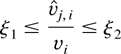
with probability one for all j ≥ 1 and i ≥ 1.
We modify the AFTER algorithm using the variance estimates. Let Wj,1 = πj as before and for n ≥ 2, let

Combine the forecasts by

.
THEOREM 2. Assume that the errors are Gaussian and that Conditions 0 and 3 are satisfied. Then the risk of the combined procedure satisfies

where C(ξ1, ξ2) = (1/ξ2 − 1 + log ξ2)/ξ12(1/ξ2 − 1)2.
Regarding the constant C(ξ1, ξ2), e.g., when ξ1 = 1/ξ2 = ½, C(ξ1, ξ2) ≈ 3.1. Note that risks of the variance estimators also appear in the preceding performance bound and thus for this combining method variance estimation is also important. However, we do not need good variance estimation for all the procedures as long as there is an accurate one for a good procedure δj. The weighting method and the risk bound suggest that procedures with bad forecasts and/or bad variance estimation receive rather small weights and accordingly have little effect on the performance of good procedures. To have good estimators of vi, assumptions on the relationship between observations are necessary. For example, one may consider stationary errors that are independent or that have short-range or long-range dependence. Performance of variance estimators can be theoretically justified under reasonable conditions. For various situations, the part of risk in the upper bound due to variance estimation in Theorem 2 may be dominated by the risk of prediction. For example, for prediction based on nonparametric regression with independent or short-range dependent errors, under mild smoothness conditions, the quantity

typically converges at a rate n−γ for some 0 < γ < 1 but

typically converges at the parametric rate 1/n. In such a case, if the number of individual forecasting procedures in Δ is finite, and if in addition the individual variance estimators converge in the sense that

holds almost surely with ξn → 1, then we again have

If no variance estimator is available from the individual forecasters, one can estimate variances based on the previous realizations of Yi and the corresponding forecasts as follows.
1. Individual variance estimation for the forecasting procedures. Fix a forecasting procedure δj. For i = 1, let

be any initial guess. For i > 1, let

Under some conditions (see Proposition 3 in the Appendix), one can show that

converges to zero in probability. Rates of convergence could also be worked out under additional conditions.
2. Estimating variance based on the combined forecasts. The combined forecasting procedure can also be used to estimate variance. For i = 1, let

be any guess. Then use this value as the variance estimate for all the forecasting procedures and accordingly assign weights by (4). For i > 1, let

Other estimators (e.g., based on exponential smoothing) may be more efficient under additional assumptions.
2.3. Combining under Non-Gaussian Errors
When there is a clear indication that the normality assumption on the conditional distributions of Yn does not hold, the combining weights should be modified. Let h(t), t ∈ R be a probability density function with mean zero and variance 1, which is thought to better capture the error distribution. Non-Gaussian choices of h allow different degrees of heavy-tailedness in the error distributions.
Condition 4. For each pair 0 < s0 < 1 and T > 0, there exists a constant B = Bs0,T (depending on s0 and T) such that
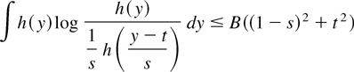
for all s0 ≤ s ≤ s0−1 and −T ≤ t ≤ T.
Note that ∫ h(y)log(h(y))/(1/s)h((y − t)/s)dy is the Kullback–Leibler divergence between density h and a rescaled and relocated density (1/s) × h((y − t)/s). Under mild conditions, this divergence should behave locally like a squared distance. The condition is satisfied by Gaussian, double-exponential, t (with degrees of freedom bigger than 2), and many other distributions.
We assume that variance estimators are available for the forecasting procedures. Note that the variance estimators given in (5) and (6) in the previous section do not require the normality assumption on the errors; thus they can be used here also. Let

for j ≥ 1 and i ≥ 1. The earlier AFTER algorithm is now modified to compute the weight based on the density function h and the variance estimates. Let Wj,1 = πj and for n ≥ 2, let

Combine the forecasts by

.
THEOREM 3. Assume that Conditions 0, 3, and 4 are satisfied. Suppose that h used in (7) indeed characterizes the distributions of the errors in the sense that for i ≥ 1, Yi has the conditional density h((y − mi)/si)/si given Zi−1 = zi−1 and Xi = xi, where

is the conditional standard deviation of Yi. Then the risk of the combined procedure satisfies

where

.
2.4. Combining under Density Forecasts
Suppose that at each time i, a forecaster δj comes up with an estimate, say,

, of pi, the conditional density of Yi given Zi−1 = zi−1 and Xi = xi. The estimate reflects the forecaster's assessment of the uncertainty in Yi prior to its occurrence. Let

be the mean of the distribution of

. Various methods have been suggested to combine probability distribution estimates (for a review on this topic, see, e.g., Genest and Zidek, 1986). Here our focus is on combining the density estimates to form a composite forecast of Y.
Let Wj,1 = πj, for n ≥ 2, let

and combine the forecasts by

.
Some technical conditions (to be given subsequently) are needed for part of the next result when

is of the form

, where gj,i is a (nonrandom) density function with mean zero and variance 1. One hopes that for at least one forecaster δj, gj,i gets closer and closer (in some sense) to pi as i → ∞.
Let F = {gθ : θ ∈ Θ} be a class of density functions on the real line. Let f be a given density (f may or may not be in F). Let D(f ∥g) denote the Kullback–Leibler divergence between two densities f and g. We say that f has a projection in F if there exists θ* ∈ Θ such that for all θ ∈ Θ, D(f ∥gθ) = D(f ∥gθ*) + D(gθ*∥gθ). The density gθ* is called the information projection of f in F. When F is an exponential family with

, where φi are linearly independent basis functions and ψ(θ) is the normalizing constant, the information projection gθ* of f exists and is characterized by ∫ φi(x) f (x) dx = ∫ φi(x)gθ*(x) dx for 1 ≤ i ≤ k (assuming that the integrals are finite) (see Csiszár, 1975).
Now let Fj,i = {gj,iμ, σ = (1/σ)gj,i((x − μ)/σ) : −∞ < μ < ∞, σ > 0} be the location-scale family generated by gj,i for j ≥ 1 and i ≥ 1. We need the following regularity condition for at least one forecasting procedure δj.
Condition 5. Suppose that at time i, the true conditional distribution of Yi has density pi = hi((yi − mi)/si)/si, where hi is a probability density function with mean 0 and variance 1 and is assumed to have an information projection in Fj,i. Assume also that the densities gj,i, i ≥ 1 satisfy Condition 4 uniformly in the sense that the constants Bs0,T in the condition do not depend on i. Assume further that there exists a constant 0 < c0 < 1 such that D(gj,iμ, σ∥gj,i) ≥ c0 min(μ2 + (σ − 1)2,1) for all i ≥ 1.
As mentioned earlier, the projection requirement in Condition 5 is satisfied if Fj,i are exponential families. The lower bound condition on the Kullback–Leibler divergence within each family is mild and typically satisfied.
THEOREM 4. Assume that Conditions 0 and 3 are satisfied.
1. In general, the risk of the combined procedure satisfies

2. For any j ≥ 1, if δj satisfies Condition 5 and D(hi∥gj, i) → 0 as i → ∞, then the risk of the combined procedure satisfies

where C is a constant depending on supi≥1 D(hi∥gj, i), τ, ξ1, ξ2, c0, and B.
Remarks.
1. Note that if a procedure δj eventually correctly specifies the distribution hi, then the projection requirement in Condition 5 is automatically satisfied for that procedure.
2. One could also use the weights in (8) to combine the density estimates. Yang (2000a, Sec. 5) gives a corresponding risk bound in terms of Kullback–Leibler divergence without the need of Conditions 0, 3, and 5.
Note that because the forms of the conditional densities hi are unknown, the combining method pays an additional price of order

. If for the forecaster δj, gj,i gets closer and closer to hi in the Kullback–Leibler divergence, then this penalty approaches zero. It may or may not affect the rate of convergence of the combined procedure, depending on how close gj,i and hi are to each other.
In particular, from the result, if there is at least one forecasting procedure that eventually picks hi with good estimates of the conditional means and standard deviations, the combined procedure based on the AFTER algorithm behaves well. Thus different distribution shapes and assumptions on the dependence relationship between the errors ei and also on the relationship between Y and the outside information X can be tried out to increase the chance of capturing the true uncertainty in Y. The theorem shows that if one such choice approximates the reality well, the combined forecast will automatically perform well.
2.5. A Consistency Property of the Combining Methods
Recall that the prediction error has a decomposition

. Equivalently, we have

This quantity measures prediction accuracy conditioning on the information available at the time. Note that it is always lower bounded by 1 and should be close to 1 for a good forecast. This motivates the following definition.
DEFINITION 2. A forecasting procedure δ with forecasts

at time i = 1,2,… is said to be consistent if

Note that from the decomposition mentioned previously, δ is consistent if and only if

which roughly means that the forecasts approach the conditional mean mi (relative to the conditional standard deviation

). This is a desirable property for a forecasting procedure.
PROPOSITION 1. Assume that the conditions for Theorems 1–3 are satisfied. Suppose that there is at least one consistent forecasting procedure in the original list. For the combining methods used in Theorems 2 and 3, we further assume that for at least one consistent forecasting procedure δj*, the variance estimator becomes more and more accurate in the sense that

. Then the combined forecasting procedure is consistent.
The proposition basically indicates that if any original procedure works well, so does the combined procedure in the consistency sense, even if nonconsistent procedures are present. Note that the key characteristic here is that the combining method does not need to know which original procedure is consistent. The conclusion of the proposition follows easily from the results of Theorems 1–3. A similar result can be derived for the combining method in Section 2.4.
2.6. Combining Forecasts without Variance Estimation
The methods in the previous sections require knowledge of the variances or appropriate estimates for determining weights for the candidate forecasts. Sometimes, e.g., when the data are nonstationary, it may be difficult to estimate the conditional variance of Yn reliably. We present a method in this section that does not require variance estimation. A key idea is borrowed from Catoni (1999).
Condition 6. Assume that the forecasts satisfy that

is bounded above by a positive constant A > 0 with probability one.
Let ψ be a fixed nonnegative convex function with ψ(0) = 0. Here ψ is not necessarily symmetric about 0. When

is used as a loss function, asymmetry of ψ is of interest to reflect the reality that over- and underforecasting might have very different consequences (cf. Newbold and Granger, 1974). Because ψ is convex, for any a0, there exists a line y = θa0(a − a0) + ψ(a0) (called a supporting line) such that ψ is above the line. We further assume subsequently that ψ is quadratically off the line and ψ does not change too dramatically in some sense. Let ψ+′ and ψ−′ denote the right and left derivatives of ψ, respectively.
Condition 7. There exist constants c > 0 and c > 0 and β > 0 such that for each a0 ∈ R and a supporting line y = θa0(a − a0) + ψ(a0) at any a0, we have

and

for each T > 0.
Condition 7 essentially restricts ψ to be basically quadratic. The slight generality is used so as to include asymmetric function

for some positive constants c1 ≠ c2. Such a loss

penalizes prediction error differently when under- or overpredicting Y.
We also need a condition on the conditional distributions of the errors. We do not require knowledge of its shape as long as certain moment generating like functions are uniformly upper bounded.
Condition 8. There exist a constant t0 > 0 and continuous functions 0 < M1(t), M2(t) < ∞ on (−t0, t0) such that for all n ≥ 1 and −t0 ≤ t ≤ t0, with probability one,

where β > 0 is the same constant as in Condition 7.
Let Wj,1 = πj and for n ≥ 2, let

where λ is a positive constant to be chosen later. Then the combined forecasting procedure δ* is defined by

.
THEOREM 5. Assume that Conditions 6–8 are satisfied. Then when λ is chosen small enough, say, 0 < λ ≤ λ0 for some constant λ0 depending on c, c, A, M1, and M2, the mean average risk (under the loss ψ) of the combined procedure satisfies

In particular, when ψ is the square loss, we have

Note that unlike the previous results, no variance estimation is required here nor is the form of the conditional distribution of Y specified. In addition, the loss (of a constant factor) beyond the additive penalty term is avoided, but under the strong moment generating function conditions. A difficulty with this method is the choice of λ, which can have a dramatic effect on the weights for moderate n. In general, the quantities A, M1, and M2 are unknown, and therefore it is hard to determine λ0. If one is willing to assume a particular form of distribution (e.g., normal), the quantities can be appropriately bounded, and then λ0 can be determined (for the regression case with independent errors, cf. Catoni, 1999). In contrast, the earlier algorithms do not require such a tuning parameter. Some simulation results in the context of nonparametric regression with independent errors in Yang (2001) suggest that when the true error distribution is double-exponential but weight calculations are based on normal error, estimation accuracy is significantly decreased. On the other hand, when both types of error distributions are considered, the combined procedure behaves as if it knew which error distribution is the correct one. Thus we tend to recommend the use of the earlier methods when one has reasonably strong confidence that some members of the chosen error distribution set closely reflect the true error distribution.
2.7. Potential Applications
2.7.1. Forecasting Based on Regression
Here we use an example to demonstrate how AFTER can be used to obtain forecasts that are adaptive to multiple scenarios.
Suppose that the response variable Yi and the outside information Xi = (Xi1,…, Xid) have the regression relationship

where m is the unknown regression function assumed to be uniformly bounded and where ei are Gaussian errors with mean zero and finite variances. Suppose that the explanatory variable X takes values in a bounded cube, which is then taken to be [0,1]d without loss of generality. In addition, we assume that the errors and Xi are independent of each other and that the unknown design density of X with respect to Lebesgue measure is bounded above and away from zero on [0,1]d. In practical situations, especially when d is large, it is usually difficult to know the form of m or how the errors are related to each other. Accordingly one may consider different scenarios in the hope that some of them capture the characteristics of the data and result in good forecasts. We consider several models/procedures here. In the first five cases, the errors are assumed to be independent. For such a scenario, as is well-known, prediction of the next response is basically equivalent to estimation of m.
1. Linear regression. Here m is assumed to be of the form

. One can use the least squares method to estimate the parameters. The squared L2 risk for estimating m is of the parametric rate 1/n if the model holds. One may also consider other plausible parametric models (e.g., including quadratic or higher order and/or cross product terms of the variables).
2. Wavelet regression. For 1 ≤ σ,q ≤ ∞ and α > 0, let Bq, σα, d(C) be the collections of all functions g ∈ Lq [0,1]d such that the Besov norm satisfies ∥g∥Bq, σα, d ≤ C (see, e.g., Triebel, 1975; DeVore and Lorentz, 1993). Besov (and similarly defined Triebel's F) classes contain a rich collection of function classes, including Sobolev classes, fractional Sobolev classes, and Hardy classes. The richness of these classes provides a great deal of flexibility (e.g., spatial inhomogeneity) for statistical function estimation. The minimax rate of convergence for estimating a function m ∈ Bq, σα, d(C) under the squared L2 loss is n−2α/(2α+d) (see, e.g., Donoho and Johnstone, 1998; Yang and Barron, 1999). For d = 1, Donoho and Johnstone (1998) show that wavelet thresholding techniques naturally lead to minimax-rate optimal estimators. Furthermore, the estimators are adaptive in the sense that the hyperparameters σ,q, and α need not be known in advance. For d > 1, one can consider tensor-product wavelet bases and expect similar minimax optimal results.
3. Tensor-product wavelets with different interaction order. Suppose d is large. When the smoothness parameter α is small or moderate, the convergence rate n−2α/(2α+d) for the Besov class Bq, σα, d(C) is slow: the phenomenon known as the “curse of dimensionality.” To overcome the “curse,” one may consider (somewhat enlarged) Besov classes of different interaction orders as follows:

Note that the simplest function class Sq, σα,1(C) contains additive functions (no interaction). These classes have different effective input dimensions (between 1 and d). By results of Yang and Barron (1999), the minimax rate of convergence under squared L2 loss for estimating m in Sq, σα, r(C) is n−2α/(2α+r) for 1 ≤ r ≤ d, as suggested by the heuristic dimensionality reduction principle of Stone (1985). Note that when r is small relative to d, the convergence rate is much improved compared with n−2α/(2α+d). Corresponding to these classes of different interaction orders, one can consider tensor-product wavelets of different interaction orders. With an appropriate thresholding, one expects to obtain an estimator that converges optimally for every Sq, σα, r(C) without knowing the hyperparameters σ, q, α, and r.
4. Neural nets. Let N(C) be the closure in L2 [0,1]d of the set of all functions g : Rd → R of the form g(x) = c0 + [sum ]i ci σ(vi′x + bi) (where the prime denotes the transpose), with |c0| + [sum ]i|ci| ≤ C, and ∥vi∥ = 1, where σ is the step function σ(t) = 1 for t ≥ 0, and σ(t) = 0 for t < 0. The minimax rate for estimating m ∈ N(C) under the squared L2 loss is shown to be bounded between

(see Yang and Barron, 1999). When d is large, the rate is slightly better than n−1/2 (independent of d), which avoids the “curse of dimensionality.” Estimators at rate O(log n/n1/2) using finite-dimensional neural network models are in, e.g., Barron (1994).
5. Kernel regression. With kernel methods, universally consistent estimators have been derived under Lq loss without any assumption on the joint distribution of (X,Y) other than the necessary existence of the corresponding moment of Y (see, e.g., Stone, 1977; Devroye and Wagner, 1980). Thus we have a consistent kernel estimator under the squared L2 loss.
Now suppose that one suspects that the random errors may be correlated. For simplicity, assume that the errors are stationary and normally distributed with Cov(ei, ei+j) of order | j|−γ for some γ > 0. When 0 < γ ≤ 1, the errors are said to be long-range dependent.
6. Prediction under long-range dependence. Suppose that the errors are long-range dependent. Then estimation of the regression function can be severely hampered (see Hall and Hart, 1990; Wang, 1996; Johnstone and Silverman, 1997; Efromovich, 1999; Yang, 1997). However, as long as the dependence parameter is known, prediction is not harder at least in terms of rate of convergence (Yang, 1997). When the dependence is unknown, the prediction problem becomes more complicated. At this point, we are not aware of general results in that direction. We here assume that γ is known and the regression function m has the neural net representation as in case 4. Then one can construct a forecasting procedure converging at rate O(n−1/2).
Now we combine the forecasts based on the preceding six cases using the method in Section 2.2. If the errors are independent, then when the true regression function is linear in the variables xi,1 ≤ i ≤ d, the prediction risk of the combined procedure converges at rate 1/n; when m is in Bq, σα, d(C) with α relatively large compared to d, the risk converges at a good rate n−2α/(2α+d); when m is in Sq, σα, r(C) for some small r, then the risk converges at rate n−2α/(2α+r); when m is not in any of these cases, but has the neural net representation, then the risk also converges at a good rate O(log n/n1/2). Even if m is not smooth at all, the combined forecasting procedure is still consistent. If the errors are long-range dependent with the dependence parameter correctly specified in case 6, and if m has the neural net representation, the risk converges at rate O(n−1/2).
The key point here is that by combining the different forecasts, the mixed forecasting procedure automatically adapts to different scenarios for a good rate of convergence.
2.7.2. Single series forecasting
For this case, one is interested in predicting a variable based on its past values. Here no outside information is used to help prediction.
Let Y1, Y2, … be a univariate time series. Different tools, including Box–Jenkins methods using ARIMA models (Box and Jenkins, 1976), exponential smoothing (e.g., Holt, 1957; Winters, 1960), and models based on, e.g., econometric theories have been proposed and widely used in practice. Note that forecasting based on ARIMA modeling typically requires selection of appropriate autoregressive, moving average, and differencing orders. As pointed out in the introduction to this paper, in the regression (and classification) context(s), it is now known that selection often causes unnecessarily large variability and does not perform as well as combining the models appropriately. It seems reasonable to expect a similar phenomenon in the time series forecasting context. Thus the AFTER algorithms could be used to combine plausible ARIMA models of different orders. Another way of using the algorithms is to combine, e.g., a forecast based on the ARIMA technique and a forecast based on exponential smoothing.
Many authors on combining forecasts have commented that one might expect a greater improvement when the procedures are more distinct in nature (see, e.g., Newbold and Granger, 1974). It may also be worthwhile to combine procedures/models of similar nature to avoid a large variability due to selection. See Zou and Yang (2003) for empirical results in that direction.
3. COMBINING FORECASTS FOR A BETTER PERFORMANCE
The results given so far deal with combining forecasts for adaptation; i.e., the purpose of combining the individual forecasts is to achieve the best overall performance over time among all the competing forecasts. In applications, the more aggressive goal of combining procedures for improving the individual forecasts is certainly appealing. See Clemen, Murphy, and Winkler (1995) for a discussion of the difference between the two directions in combining forecasts.
In this section, we consider linear combinations of forecasts with a certain constraint. The treatment is mainly theoretical because the combining methods we study are hard to implement in applications. Our purpose is to address several important issues on combining forecasts for a better performance. The theoretical understanding can be very helpful when evaluating practically feasible combining methods. Related theoretical results on linearly combining nonparametric regression procedures with independent errors are in Juditsky and Nemirovski (2000) and Yang (in press). Some practical combining methods for regression have been proposed by Wolpert (1992), Breiman (1996a), and LeBlanc and Tibshirani (1996).
Let Δ = {δ1, δ2,…} be the set of original forecasting procedures. One hopes that a certain linear combination of them will significantly outperform any of the individual procedures. There are two related issues that we want to address:
1 stability versus pursuing further improvement;
2. sparsity in combining.
In addition to higher computational cost, there must also be a price in terms of statistical performance for searching for the best linearly combined procedure. The price will be quantified in a minimax framework in terms of the number of procedures being combined. As intuition suggests, the more procedures involved in combining, the bigger the price one needs to pay as a result of the increased variability of the combined forecast. The first issue then amounts to the comparison of the potential gain and the price of combining more forecasting procedures. If the potential gain is larger than the price, then there is an advantage in combining more procedures (ignoring the computational cost). Of course, in applications, one does not know the optimal trade-off between the potential gain and the price. Thus it would be nice to have a combined procedure that automatically behaves the right way: that would be both conservative (which targets the best performance based on a small number of procedures to avoid a large variability) and aggressive (which targets the best performance based on a large number of procedures to increase the potential gain), whichever is better. Sparseness in combining is also an important issue. If many coefficients in a linear combination of the procedures are rather small, keeping the important ones only can lead to a much better performance because of the much reduced variability of the resulting forecast. Because one does not know which coefficients are important in advance, some sort of search over sparse combinations is needed.
Empirical evidence suggests that simple combining methods sometimes outperform more complicated versions. A possible explanation, as proposed by several researchers (e.g., Figlewski and Urich, 1983; Kang, 1986; Clemen and Winkler, 1986), is that more complicated combining methods have a much larger variability. Our theoretical results tend to support this view.
For simplicity in illustration, in this section we will assume normality of the conditional distributions of the future response given the past data and the present outside information and will also assume that the variances vi are known and bounded above and below by some positive constants as in Corollary 1. However, similar results can be obtained with little difficulty for the other cases considered in Section 2 with weaker assumptions.
3.1. What Is the Price of Linearly Combining for Improvement?
Let Δ = {δ1,…, δM} be a finite collection of forecasting procedures with δj producing forecast

at time i. Consider the linear combination of the procedures:
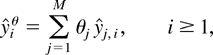
where θ = (θ1,…, θM) satisfies the constraint

. Let δθ denote the corresponding forecasting procedure and let Θ = ΘM denote the set of all such θ. Let θ* be the minimizer of

over θ ∈ Θ and let R(M; n;Δ) denote the minimized value. It captures the best performance among all the linearly combined procedures subject to the constraint. Targeting δθ* (which is unknown), we combine the procedures δθ using the AFTER algorithm with θ restricted to a finite set ΘD ⊂ Θ. An appropriate choice of ΘD (see the proof of Theorem 6 in the Appendix) leads to the following result. Let δM denote the combined forecasting procedure. Recall that for a forecasting procedure δ with forecast

is the mean average square risk.
THEOREM 6. Assume that Conditions 1 and 2 are satisfied. The risk of the combined procedure δM can be bounded as follows:

where C is a constant depending on A1, A2, and A3 (as in Conditions 1 and 2). In particular, if M = Mn ≤ C0 nτ for some τ > 0 and C0 > 0, then

where the constant C′ depends on A1, A2, A3, and C0.
Remark. A similar result in the regression context suitable when

is given in Juditsky and Nemirovski (2000).
The result characterizes the performance of the combined procedure in terms of the best linear combination (subject to the constraint) and a penalty. For nonparametric estimation or prediction, exact risks are usually too difficult to obtain without restrictive conditions, and accordingly convergence rates are used to compare procedures. The result implies that when combining M = C0 nτ procedures, the combined forecast has mean average risk converging at the rate of the best combination plus a penalty term or price, which is of order (τ log n/n)1/2 when τ ≥ ½ and is of order n−(1−τ) log n when 0 ≤ τ < ½.
Define

Note that ψn(M) is the penalty term associated with the combined procedure for not knowing which linear coefficients work the best. The term ψn(M) increases as M increases and thus can be viewed as a complexity penalty of combining M procedures (relative to the sample size). When n is small, the price of combining a large number of procedures is very high, but when n becomes large, more forecasts can be combined for a relatively low price.
One might wonder if the price we gave previously for combining forecasts is really necessary or rather is due to suboptimal combining. In fact, the upper bound given previously is almost optimal in the sense that it cannot be improved much in general as shown in the following result. For simplicity, assume that the conditional variance of Yi given zi−1 and xi is 1 for i ≥ 1. For a real number a, let [lfloor ]a[rfloor ] denote the largest integer no bigger than a.
THEOREM 7. Consider Mn = [lfloor ]nτ[rfloor ] for some τ > 0. There exist Mn procedures ΔMn = {δj,1 ≤ j ≤ Mn} satisfying Condition 2 such that for any combined procedure δ based on ΔMn, one can find a case of true data generating process such that

where the constant C″ does not depend on n.
Thus no matter how carefully a combining procedure is constructed, it cannot be uniformly close to the ideal performance R(M; n;ΔMn) within an order smaller than the one given earlier. Note that the lower rate matches the upper rate in Theorem 6 when τ > ½ and the upper and lower rates differ only in logarithmic factors when 0 ≤ τ ≤ ½.
Theorems 6 and 7 together with Corollary 1 provide some understanding of the question of whether one should combine for adaptation or combine for improvement. By Corollary 1, and taking the uniform prior weight on the Mn procedures, combining for adaptation yields risk of order

If Mn does not increase exponentially fast, log Mn /n is of order log n/n, which is usually negligible for nonparametric estimation or prediction. Then combining for adaptation achieves the best performance (rate) among the Mn forecasting procedures. In terms of rate of convergence of the mean average risk, linearly combining nτ procedures for better performance is guaranteed to do better than combining for adaptation only when both R(Mn; n;ΔMn) and the penalty term (log n/n)1/2 for τ > ½ and n−(1−τ) for 0 ≤ τ ≤ ½ converge at a faster rate than inf1≤j≤Mn R(δj; n) + (log Mn)/n. Otherwise, the linearly combined procedure can do worse or even much worse than combining for adaptation. Thus it is not automatically advantageous to combine forecasting procedures for improvement.
Theorems 6 and 7 can also help us to understand how many procedures should be combined. Note that inf1≤j≤Mn R(δj; n) is nonincreasing as more forecasting procedures are included in Δ, but on the other hand the penalty ψn(Mn) increases. Thus one needs a good trade-off between the potential gain and the complexity penalty. In the next section, a method will be given to automatically achieve the best trade-off.
3.2. Combining with Multiple Discretization Accuracies
In the construction of the combined forecast in the previous section, a discretization is used that is chosen according to n (among other things). This is undesirable because it requires knowledge of how many times one will forecast in the future. Theoretically speaking, the problem can be fixed by considering different discretization accuracies at the same time. In addition, we will seek automatic balance between the potential gain and the complexity penalty.
Let Δ = {δ1, δ2,…} be a list of forecasting procedures. Let ΔM = {δ1, δ2,…, δM}. Fix M for the time being. For each k ≥ 1, consider a best ε-net Nk (under the l1M distance) in ΘM with 2k points (which minimizes the maximum distance between a point in ΘM and the closest point in the net). From Schütt (1984, Theorem 1), the entropy number under the l1M distance is upper bounded by cφ(M, k), where

and c does not depend on M or k. We combine the 2k corresponding forecasting procedures (linear combinations of the original M procedures with θ in Nk) for adaptation using the uniform prior weight. Denote the procedure by δ(M, k). By Corollary 1,

where C is a constant depending on A1, A2, and A3. For convenience, we will use the same symbol C to denote any constant that may depend on A1, A2, and A3.
Define log* by log* x = log(x + 1) + 2 log log(x + 1). Now we combine the procedures {δ(M, k) : M ≥ 1, k ≥ 1} for adaptation with the prior weight ce−log*M−log*k, where the constant c is chosen to normalize the weights to sum to 1. Let δ* denote this forecasting procedure. It follows again from Corollary 1:

Compared with the other terms, (log M/n) + (log k/n) are asymptotically negligible. Thus the final combined procedure behaves automatically as well as if it knew the optimal discretization accuracy that balances k/n and φ2(M, k) and knew also the optimal number of procedures Mn that balances R(M; n;ΔM) and infk((k/n) + φ2(M, k)). In particular, for each n and M, by taking k as in the proof of Theorem 6, we have

Note that the upper bound agrees in order with that in Theorem 6 but the combining procedure does not need to know n in advance. Up to a constant factor, the combined forecast automatically achieves the best trade-off between risk reduction and the complexity penalty for combining.
3.3. Sparsely Combining
In some cases, when combining many procedures, the best linear combination may concentrate on only a few of them. For such a case, combining only the important procedures leads to a much better performance because of the significantly reduced variability in the final combined procedure. Usually one does not know which of the original procedures are important individually, and even if one does, some of the individually important procedures may not be needed in the best linear combination. Without such knowledge, we consider different sparse combinations of the candidate forecasts.
The idea is to combine each suitable subset of the candidate procedures for improvement and then combine the new ones for adaptation (over the different subsets). For each integer M > 1, 1 ≤ L < M, and a subset S of {1,2,…, M} of size L, let δ(S) be the linearly combined (for improvement) procedure based on {δj : j ∈ S} using multiple discretization accuracies as in the construction of δ* in the previous section. Then let δM, L be the combined (for adaptation) procedure based on all such δ(S) with the uniform prior weight

(there are

many such procedures). Then let δ(M) be the combined (for adaptation) procedure based on δM,1,…, δM, M−1 using the uniform prior weight 1/(M − 1). Let δF* denote the combined (for adaptation) procedure based on δ(M), M ≥ 2 with the prior weight c′ exp(−log* M), where the constant c′ is chosen such that

. Let Δ(S) denote the collection of procedures {δj : j ∈ S}. Based on Corollary 1, we have

Compared with upper bound (13), we see the potential advantage of sparse combining. Let Mn achieve the best trade-off between R(M; n;ΔM) and ψn(M). Suppose there exists Δ(S) ⊂ {1,2,…, Mn} with L = |Δ(S)| much smaller than Mn and R(Mn; n;Δ(S)) is only slightly larger than R(Mn; n;ΔM). Then ψn(L) + (L log Mn)/n is much smaller than ψn(Mn) if Mn does not grow exponentially fast. For such a case, sparse combining avoids unnecessarily large variability in combining all the first Mn procedures.
Sparse approximation/estimation has been effectively used for wavelet estimation (see, e.g., Donoho and Johnstone, 1994, 1998; Johnstone, 1999) and also has been applied to general model selection (see Yang and Barron, 1998, 1999; Barron, Birgé, and Massart, 1999).
3.4. Adaptively Combining Forecasts
The results in the previous sections provide helpful insight into the difference between combining for adaptation and combining for improvement; on potential gain and the price of combining forecasts; and on the advantage of sparse combining. In practice, however, one does not know which scenario one is in and therefore can not gauge beforehand the optimal combining strategy. If one indiscriminately combines a large number of procedures, one might end up with a much worse performance compared with combining for adaptation. In this section, we give an adaptive combining method that overcomes these difficulties, at least in theory. Here we show that when combining the procedures properly, one can have the potential of obtaining a large gain in forecasting accuracy yet without losing much when there happens to be no advantage in considering sophisticated linear combinations for improvement.
Consider three different approaches for combining procedures in Δ = {δ1, δ2,…}.
The first approach is to combine the procedures for adaptation. Here one intends to capture the best performance (in terms of rate of convergence) among the candidate procedures. Let δA* denote this combined procedure based on Δ using the AFTER algorithm as given in Section 2. When Δ is not a finite collection, one cannot use uniform prior weight. One choice of prior weight πj is ce−log* j, where the constant c is chosen to normalize the weights to sum to 1. Based on Corollary 1, we have

If one procedure, say, δj*, behaves the best asymptotically, then the penalty is of order 1/n. If the best procedure changes according to n, then infj(log(j + 1)/n + R(n;δj)) is a trade-off between complexity and estimation accuracy.
The second approach targets the best performance among all the linear combinations of the original procedures up to different orders. This is the combining procedure described in Section 3.2. Let δB* denote this procedure. Then

The third approach is to combine the procedures through various sparse combinations as described in Section 3.3. Let δC* denote this procedure. Then

Now we combine these three procedures δA*, δB*, and δC* with equal prior weight 1/3 and let δF denote the final combined procedure. Note that this is still a linear combination of the original procedures. We have the following conclusion.
PROPOSITION 2. Assume Conditions 1 and 2 are satisfied. Then the combined procedure satisfies

where C is a constant depending only on A1, A2, and A3.
Thus in terms of rate of convergence, first of all, the combined forecasting procedure converges as fast as any original procedure. Second, when linear combinations of the first Mn procedures (for some Mn > 1) can improve estimation accuracy dramatically, one pays a price at most of order ψn(Mn) for the better performance. When certain linear combinations of a small number of procedures perform well, the combined procedure can also take advantage of that. In summary, the combined procedure is automatically both aggressive in pursuing greater accuracy improvement and conservative in avoiding paying a price higher than the potential gain.
4. CONCLUDING REMARKS
Combining forecasts is a useful technique for sharing strengths of different forecasting procedures. There are two closely related directions in combining forecasts: combining for adaptation and combining for improvement.
An algorithm, AFTER, is proposed for combining forecasts for adaptation. The method assigns weights to the candidate procedures according to their performances thus far and relies on the specification of the forms (e.g., Gaussian or double-exponential) of the conditional distributions of Y given the past data and the current outside information. One may use a fixed specification for combining or use specifications from the individual forecasters. When the common specification for the first case or the individual specifications corresponding to the best forecasts capture the true uncertainty in Y well, the AFTER algorithm is shown to have a prediction risk automatically close to the best procedure. No assumption on the relationship between different forecasts is needed for the result. In applications, various model assumptions on the relationship between Y and the outside information X and on dependence structure among the errors (noise) can be considered in constructing individual predictions. The resulting forecasts and also additional forecasts based on subjective assessments can be combined. The algorithm AFTER is easy to implement in practice. Combining without specifying or estimating the conditional distributions of Y is also studied under assumptions on certain moment generating functions.
An alternative to combining procedures is selecting the best one. Model selection criteria can be used in that regard when combining model-based forecasts. However, model selection is often unstable, which causes a rather large variability in prediction. Combining with appropriate weighting as by AFTER gives more stable predictions and accordingly yields better performance.
In the other direction, we studied linearly combining (subject to a constraint) forecasts for improving the individual procedures. Because the “optimal” weights are estimated, one must pay a price in the sense that the risk of the combined forecast is larger in general than that of the best linear combination. The potential gain and the price in terms of prediction accuracy are theoretically quantified. The result supports the empirical finding that combining does not necessarily lead to performance improvement and indiscriminate combining of a number of forecasts can have a much worse performance compared to the best individual procedure. In addition, we showed an advantage of sparse combining. A multipurpose combining method is shown to be able to automatically balance the potential gain and the complexity penalty; it takes advantage of sparse combining when only a few procedures have large weights for the best linear combination; and it always achieves (in rate) the best individual performance.
Our results on linearly combining forecasts for improvement are mainly theoretical. Computationally feasible methods need to be developed with similar properties. In addition to linear combining, nonlinear methods may also prove helpful for sharing strengths of different procedures. Another interesting and challenging research direction is combining prediction intervals. See Taylor and Bunn (1999) for some simulation results. Further theoretical research on these topics, in our opinion, will be a fruitful guide for combining forecasts in practice.
APPENDIX: PROOFS OF THE RESULTS
Proof of Theorem 1. Let

Consider log(fn/qn). By monotonicity of the log function, for each fixed j* ≥ 1, we have

On the other hand, observe

Let

. It follows by definition of Wj,i that

. Together with (A.1), we have

Taking expectation on both sides of (A.2) under the conditional distribution of Yn given Zn−1 = zn−1 and xn, we have

Because yn = mn + en, where En en = 0, we have

It follows that

Observe that under the normality assumption on the errors,

where the inequality is the familiar relationship between the Kullback–Leibler divergence and the squared Hellinger distance. Let

denote the means and variances of pn and gn, respectively. Under Condition 0, it can be easily verified that

. Observing that

, together with Lemma 1, which follows, we have that

It follows that

Together with (A.3), we have

Thus

Handle

the same way as for i = n, and similarly for other 1 ≤ i < n − 1, we have

Because the preceding analysis holds for every j*, it follows that

The conclusion of Theorem 1 then follows. This completes the proof of Theorem 1. █
Proof of Theorem 2. We only need to modify the proof of Theorem 1. Define fn as before but modify qn to be

As before, for each fixed j* ≥ 1, we have

Taking expectation conditioned on zi−1 and xi, we have

Similarly as before,

, where gi is modified to be

Together with (A.4) and (A.5), we have

Notice that as before

, and using the fact that vgi ≤ ξ2 vi + 4viτ and applying Lemma 1, we have

Together with (A.6), we have

It is straightforward to verify that if x ≥ x0 > 0, x − 1 − log x ≤ cx0(x − 1)2 for a constant cx0 = (x0 − 1 − log x0)/(x0 − 1)2. Together with the fact that the preceding inequality holds for every j*, under Condition 3, it follows that

where C(ξ1, ξ2) = (1/ξ2 − 1 + log ξ2)/ξ12(1/ξ2 − 1)2. The conclusion then follows. This completes the proof of Theorem 2. █
Proof of Theorem 3. Redefine

Similarly as before, we have that for every j*,

By a simple linear transformation,

where for the last inequality, we use Condition 4 with s0 = min(ξ11/2, ξ2−1/2) and T = τ1/2. It follows that

The rest of the proof then follows easily. This completes the proof of Theorem 3. █
Proof of Theorem 4. We prove the first part of the result first. Let Πi=1npi be the true joint distribution of Y1,…,Yn and

be the estimated version of forecaster j for j ≥ 1. Let

. Then as before, for each j* ≥ 1,

Let

for i ≥ 1. By definition of Wj,i, qn(y1,…, yn) = Πi=1ngi(yi). Thus

Then lower bounding the Kullback–Leibler divergence by the squared Hellinger distance and applying Lemma 1 as in the proof of Theorem 1, we have

For the second result of the theorem, let

For δj satisfying Condition 5, taking expectation conditioned on zi−1 and xi, by a simple linear transformation and then applying Lemma 2 (which follows), we have

where C is a constant depending on c0 and Bs0,T with s0 and T being constants depending on ξ1, ξ2, and τ. Then as before, we have

The conclusion then follows. This completes the proof of Theorem 4. █
Proof of Theorem 5. Define h(x) = exp(−λψ(x)) (it is not necessarily a probability density function). Define

For each fixed j* ≥ 1, we have

As before,

It follows that

We now bound

, where EJ (depending on i) denotes expectation with respect to J under the probability mass function P(J = j) = Wj,i (for a fixed i). By Lemma 10.1 of Catoni (1999), under (10) of Condition 7, we have

where I denotes

For handling the term I, note that by (10) of Condition 7,

Under (9) of Condition 7, let

; we have

Taking expectation under EJ, we have

Observing that

by definition of

, we have

It follows that the term I is bounded by

multiplied by

Under Condition 8, by taking conditional expectation given zi−1 and xi, we have that when cλ2β ≤ t0,

Take λ small enough, say, 0 < λ ≤ λ0, so that λ2c222β−2ecλ2β(A+1)β((A + 1)2β × M2(cλ2β) + M1(cλ2β)) ≤ λc/2 and cλ2β ≤ t0. Together with (A.13),

It follows that

where the last step follows from

by Jensen's inequality based on convexity of ψ. Together with (A.9) and (A.8), we have

Because j* is arbitrary, we have

This completes the proof of Theorem 5. █
Proof of Theorem 6. We consider first the case when

. Recall

. Let Nε be an ε-net in ΘM under the l1M distance; i.e., for each θ ∈ ΘM, there exists θ′ ∈ Nε such that

. An ε-net Nε in ΘM yields a suitable net in the set F = {δθ : θ ∈ ΘM} of the linear combinations of the original forecasts. Let

denote the original forecasts by the M procedures at time i. Let Fε be the set of the linear combinations of the forecasts

with coefficients in Nε. Then for any

with θ ∈ ΘM, there exists θ′ ∈ Nε such that

where A3 is an upper bound on the magnitude of the original forecasts. Now we combine all the procedures in Fε using the AFTER algorithm given in Section 2 for Theorem 1 with the uniform prior weight 1/|Nε|. Let

denote the combined forecasts at time i. By Corollary 1, we have

where C depends only on A1, A2, and A3. Because Fε is an (A3ε)-net in F, by the triangle inequality, for any set of mi, we have

. It follows that

To get the best upper bound (in order), we need to minimize log(|Nε|) + 2A32ε2n when discretizing ΘM. We apply a result on entropy number, i.e., the worst case approximation error with the best net of size of 2k points. Let εk denote the entropy number of ΘM under the l1M distance. From Schütt (1984, Theorem 1), when k ≥ M, εk ≤ c2−k/M for some constant c independent of k and M. Take

(note that k ≥ M). (Strictly speaking, we need to round up to make k an integer.) Then

where c′ depends only on A3 and c. The upper bound in Theorem 6 for

then follows.
Now consider the other case:

. The preceding argument leads to a suboptimal rate M log(1 + n/M) for M ≤ n. For this case, as a result of the l1 constraint, the number of large coefficients is small relative to M when

. Working with only the large coefficients can result in the optimal rate of convergence.
Note that for

. Then by a sampling argument (see, e.g., Barron, 1993, Lemma 1) for each m, there exist a subset I ⊂ {1,…, M} of size m and θI′ = (θi′, i ∈ I) such that

. Taking

, we have

. Consider an ε-net in BI = {θI : [sum ]j∈I|θj| ≤ 1} under the l1m* distance. Again by Schütt (1984, Theorem 1), taking k = [m*(log(n/m*) + 2 log 2)]/2 log 2, the best ε-net has approximation accuracy

. Then as in (A.14), we know that there exists θI′′ in this ε-net such that

. Thus for each δθ ∈ F, there exist I* ⊂ {1,…, M} of size m* and θI′′ such that

where c′′ depends only on A3 and c.
Now for each fixed subset I ⊂ {1,…, M} of size m*, discretize the linear coefficients as described earlier. Then (with the uniform prior weight) combine the corresponding linear combinations of the forecasting procedures in Δ. Then combine these (combined) procedures over all possible choices of I (there are

many such I altogether) with the uniform prior weight. Let δM denote this final procedure and let ΔI = {δi, i ∈ I}. Applying Corollary 1 twice, we have that

where the constants C and C′ depend on A1, A2, and A3. This completes the proof of Theorem 6. █
Proof of Theorem 7. Let Xi = (Xi1,…, XiM), i ≥ 1 be independent and identically distributed (i.i.d.) where Xi1,…, XiM are independent and uniformly distributed on [0,1]. Assume Yi = f (Xi) + ei, where the errors ei are independent and normally distributed with mean zero and variance 1. Let φ1(x), …, φM(x) be uniformly bounded orthonormal basis functions (e.g., trigonometric basis). Take δi, i ≥ 1 to be the procedure that forecasts Yi by φi(Xi). For each M = nτ, consider the class of regression functions

. It is clear that

. For this case, because of the independence of the errors, prediction and regression are essentially identical. The conclusion of Theorem 7 then follows from Theorem 2 of Yang (in press). This completes the proof of Theorem 7. █
The following lemma relates the Hellinger distance between two densities to their means and variances.
LEMMA 1. Let p and g be two probability densities on the real line with respect to a measure ν, with means μp and μg, variances 0 < σp2 < ∞ and 0 < σg2 < ∞, respectively. Then

When dH2(p, g) ≤ ½, we have

Proof. Let a be any constant. Note that

where the last step follows from the Cauchy–Schwarz inequality. Observe that

By taking a = (μp + μg)/2 (the mean of (pn + gn)/2), we have that ∫(x − a)2((p + g)/2)dν is the variance of the distribution (p + g)/2, which is denoted by σ(p+g)/22. Then with some elementary calculations, we have that

From the preceding analysis, we have

The second conclusion follows easily. This completes the proof of Lemma 1. █
LEMMA 2. Let f and g be two probability densities on the real line (with respect to a measure ν), both with mean 0 and variance 1. Suppose f has an information projection in the location and scale family F = {(1/σ)g((x − μ)/σ) : −∞ < μ < ∞, σ > 0}. Suppose that the density g satisfies Condition 4 and assume further that there exists a constant 0 < c < 1 such that D(gμ, σ∥g) ≥ c min(μ2 + (σ − 1)2,1) holds for all −∞ < μ < ∞ and σ > 0, where gμ, σ = (1/σ)g((x − μ)/σ). Then when D(f ∥g) ≤ c/2, for |μ| ≤ a and 1/b ≤ σ ≤ b for some constants a > 0 and b > 1, we have

for some constant C > 0 depending only on c and Bs0,T with

.
Proof. Under the assumption of information projection, we have the following Pythagorean decomposition:

for some −∞ < μ* < ∞, and σ* > 0. It follows that D(f ∥gμ*, σ*) ≤ D(f ∥g) and D(gμ*, σ*∥g) ≤ D(f ∥g). Under the assumptions on g, the latter inequality implies that when D(f ∥g) ≤ c/2, we have

Then

. Under Condition 4 on g, with a simple linear transformation, we have

where

(because

). By triangle inequality,

Thus when D(f ∥g) ≤ c/2, we have

Then

where

. Together with earlier inequalities, we have that when D(f ∥g) ≤ c/2,

This completes the proof of Lemma 2. █
For the next result, consider the setup in the introduction to this paper. Let

be a filtration. Assume that the errors ei form a martingale difference relative to the filtration; i.e., for i ≥ 1, ei is

measurable and

almost surely. Clearly ei has mean zero and conditional variance

for i ≥ 1. Let δ be a forecasting procedure producing forecasts

at time 1,2, and so on. We “estimate” vi by

prior to observing Yi. The following proposition gives a property of this estimator.
PROPOSITION 3. Assume that ei have uniformly bounded fourth moments and

. In addition, we assume that vi converges to a positive random variable v with probability one. If δ is consistent (as defined in Section 2.5), then

converges in probability to zero.
Remark. Clearly the conditions on the errors are satisfied if they are i.i.d. with a finite fourth moment.
Proof. Expanding squares, we have

It follows then that

Note that

and for l1 > l2,

It follows that

and similarly

Therefore

It follows that

converges in probability to zero. Because δ is a consistent forecasting procedure, by Markov inequality, we have for any ε > 0,

Together with the assumption that vl converges almost surely to v > 0, it can be easily shown that

in probability. Again because vl converges to v with probability one, we have

almost surely. Together with (A.16), we have

This completes the proof of Proposition 3.
References
REFERENCES
Armstrong, J.S.
(1989)
Combining forecasts: The end of the beginning or the beginning of
the end?
International Journal of Forecasting
5,
585–588.Google Scholar
Barron, A.R.
(1993)
Universal approximation bounds for superpositions of a sigmoidal
function.
IEEE Transactions on Information Theory
39,
930–945.Google Scholar
Barron, A.R.
(1994)
Approximation and estimation bounds for artificial neural networks.
Machine Learning
14,
115–133.Google Scholar
Barron, A.R.,
L. Birgé, &
P. Massart
(1999)
Risk bounds for model selection via penalization.
Probability Theory and Related Fields
113,
301–413.Google Scholar
Barron, A.R.,
J. Rissanen, &
B. Yu
(1998)
The minimum description length principle in coding and modeling.
IEEE Transactions on Information Theory
44,
2743–2760.Google Scholar
Bates, J.M. &
C.W.J. Granger
(1969)
The combination of forecasts.
Operational Research Quarterly
20,
451–468.Google Scholar
Box, G.E.P. &
G.M. Jenkins
(1976)
Time Series Analysis: Forecasting and Control,
2nd ed.
Holden-Day.
Buckland, S.T.,
K.P. Burnham, &
N.H. Augustin
(1997)
Model selection: An integral part of inference.
Biometrics
53,
603–618.Google Scholar
Catoni, O.
(1999)
“Universal” Aggregation Rules with Exact Bias Bounds.
Preprint no. 510,
Laboratoire de Probabilites et Modeles Aleatoires, Université
Paris VI & Université Paris VII.
Cesa-Bianchi, N.,
Y. Freund,
D.P. Haussler,
R. Schapire, &
M.K. Warmuth
(1997)
How to use expert advice?
Journal of the Association for Computing Machinery
44,
427–485.Google Scholar
Chatfield, C.
(1995)
Model uncertainty, data mining, and statistical inference (with
discussion).
Journal of the Royal Statistical Society, Series A
158,
419–466.Google Scholar
Clemen, R.T.
(1989)
Combining forecasts: A review and annotated bibliography.
International Journal of Forecasting
5,
559–583.Google Scholar
Clemen, R.T.,
A.H. Murphy, &
R.L. Winkler
(1995)
Screening probability forecasts: Contrasts between choosing and
combining.
International Journal of Forecasting
11,
133–145.Google Scholar
Clemen, R.T. &
R.L. Winkler
(1986)
Combining economic forecasts.
Journal of Business and Economic Statistics
4,
39–46.Google Scholar
Cover, T.M.
(1965)
Behavior of sequential predictors of binary sequences. In
Transactions of the Fourth Prague Conference on Information Theory,
Statistical Decision Functions, and Random Processes, pp.
263–271.
Publishing House of the Czechoslovak Academy of Sciences.
Csiszár, I.
(1975)
I-Divergence geometry of probability distributions and minimization
problems.
Annals of Probability
3,
146–158.Google Scholar
Dawid, A.P.
(1984)
Present position and potential developments: Some personal views.
Statistical theory—The prequential approach (with
discussion).
Journal of the Royal Statistical Society, Series A
147,
278–292.Google Scholar
DeVore, R.A. &
G.G. Lorentz
(1993)
Constructive Approximation.
Springer.
Devroye, L.P. &
T.J. Wagner
(1980)
Distribution-free consistency results in nonparametric
discrimination and regression function estimation.
Annals of Statistics
8,
231–239.Google Scholar
Donoho, D.L. &
I.M. Johnstone
(1994)
Ideal denoising in an orthonormal basis chosen from a library of
bases.
C.R. Acad. Sci. Paris
319,
1317–1322.Google Scholar
Donoho, D.L. &
I.M. Johnstone
(1998)
Minimax estimation via wavelet shrinkage.
Annals of Statistics
26,
879–921.Google Scholar
Efromovich, S.
(1999)
How to overcome curse of long-memory?
IEEE Transactions on Information Theory
45,
1735–1741.Google Scholar
Figlewski, S. &
T. Urich
(1983)
Optimal aggregation of money supply forecasts: Accuracy,
profitability, and market efficiency.
Journal of Finance
28,
695–710.Google Scholar
Genest, C. &
J.V. Zidek
(1986)
Combining probability distributions: A critique and an annotated
bibliography.
Statistical Science
1,
114–148.Google Scholar
Gouriéroux, C. &
A. Monfort
(1992)
Qualitative threshold ARCH models.
Journal of Econometrics
52,
159–199.Google Scholar
Hall, P. &
J.D. Hart
(1990)
Nonparametric regression with long-range dependence.
Stochastic Processes and Their Applications
36,
339–351.Google Scholar
Haussler, D.,
J. Kivinen, &
M.K. Warmuth
(1998)
Sequential prediction of individual sequences under general loss
functions.
IEEE Transactions on Information Theory
44,
1906–1925.Google Scholar
Hoeting, J.A.,
D. Madigan,
A.E. Raftery, &
C.T. Volinsky
(1999)
Bayesian model averaging: A tutorial (with discussion).
Statistical Science
14,
382–401.Google Scholar
Holt, C.C.
(1957)
Forecasting Seasonals and Trends by Exponentially Weighted Moving
Averages.
Carnegie Institute of Technology.
NR Research Memorandum 52.
Johnstone, I.
(1999)
Function Estimation in Gaussian Noise: Sequence Models.
Manuscript.
Johnstone, I. &
B.W. Silverman
(1997)
Wavelet threshold estimators for data with correlated noise.
Journal of the Royal Statistical Association, Series B
59,
319–351.Google Scholar
Juditsky, A. &
A. Nemirovski
(2000)
Functional aggregation for nonparametric estimation.
Annals of Statistics
28,
681–712.Google Scholar
Kang, H.
(1986)
Unstable weights in the combination of forecasts.
Management of Science
32,
683–695.Google Scholar
Leamer, E.E.
(1978)
Specification Searches: Ad hoc Inference with Nonexperimental Data.
Wiley.
LeBlanc, M. &
R. Tibshirani
(1996)
Combining estimates in regression and classification.
Journal of the American Statistical Association
91,
1641–1650.Google Scholar
Littlestone, N. &
M.K. Warmuth
(1994)
The weighted majority algorithm.
Information and Computation
108,
212–261.Google Scholar
Merhav, N. &
M. Feder
(1998)
Universal prediction.
IEEE Transactions on Information Theory
44,
2124–2147.Google Scholar
Newbold, P., &
C.W.J. Granger
(1974)
Experience with forecasting univariate times series and the
combination of forecasts.
Journal of the Royal Statistical Society, Series A
137,
131–165 (with discussion).Google Scholar
Ploberger, W. &
P.C.B. Phillips
(1999)
Empirical Limits for Time Series Econometric Models.
Cowles Foundation Discussion paper 1220,
Yale University.
Rissanen, J.
(1986)
Stochastic complexity and modeling.
Annals of Statistics
14,
1080–1100.Google Scholar
Schütt, C.
(1984)
Entropy numbers of diagonal operators between symmetric Banach
spaces.
Journal of Approximation Theory
40,
121–128.Google Scholar
Stone, C.J.
(1977)
Consistent nonparametric regression.
Annals of Statistics
5,
595–620.Google Scholar
Stone, C.J.
(1985)
Additive regression and other nonparametric models.
Annals of Statistics
13,
689–705.Google Scholar
Taylor, J.W. &
D.W. Bunn
(1999)
Investigating improvements in the accuracy of prediction intervals
for combinations of forecasts: A simulation study.
International Journal of Forecasting
15,
325–339.Google Scholar
Triebel, H.
(1975)
Interpolation properties of ε-entropy and diameters. Geometric
characteristics of embedding for function spaces of Sobolev-Besov type.
Mat. Sbornik 98, 27–41;
English trans. in Math. USSR Sb. 27, 23–37,
1977.Google Scholar
Wang, Y.
(1996)
Function estimation via wavelet shrinkage for long-memory data.
Annals of Statistics
24,
466–484.Google Scholar
Vovk, V.G.
(1990)
Aggregating strategies. In
M. Fulk &
J. Case (eds.),
Proceedings of the Third Annual Workshop on Computational Learning
Theory, pp.
372–383.
Winters, P.R.
(1960)
Forecasting sales by exponentially weighted moving averages.
Management of Science
6,
324–342.Google Scholar
Yang, Y.
(1997)
Nonparametric Regression and Prediction with Dependent Errors.
Technical Report 29,
Department of Statistics, Iowa State University.
A shorter version appeared in Bernoulli 7, 633–655, 2001.
Yang, Y.
(in press)
Aggregating regression procedures for a better performance.
Bernoulli,
forthcoming.
Yang, Y.
(2000a)
Mixing strategies for density estimation.
Annals of Statistics
28,
75–87.Google Scholar
Yang, Y.
(2000b)
Combining different procedures for adaptive regression.
Journal of Multivariate Analysis
74,
135–161.Google Scholar
Yang, Y.
(2000c)
Adaptive estimation in pattern recognition by combining different
procedures.
Statistica Sinica
10,
1069–1089.Google Scholar
Yang, Y.
(2001)
Adaptive regression by mixing.
Journal of the American Statistical Association
96,
574–588.Google Scholar
Yang, Y.
(2003)
Regression with multiple candidate models: Selecting or mixing?
Statistica Sinica
13,
783–809.Google Scholar
Yang, Y. &
A.R. Barron
(1998)
An asymptotic property of model selection criteria.
IEEE Transactions on Information Theory
44,
95–116.Google Scholar
Yang, Y. &
A.R. Barron
(1999)
Information-theoretic determination of minimax rates of convergence.
Annals of Statistics
27,
1564–1599.Google Scholar
Zou, H. &
Y. Yang
(2003)
Combining time series models for forecasting.
International Journal of Forecasting,
forthcoming.Google Scholar
 You have
Access
- 152
- Cited by