1. Introduction
The mathematical literature applied to biology and social science is rich of models devoted to the description of aggregation. Motivations come from several problems like embryo development, tissue homeostasis, tumor growth, animal swarming, and flocking. The literature presents heterogeneous mathematical tools: discrete and continuous individual-based models, ordinary and partial differential equations (ODEs and PDEs) and a mixture of the two. Also, because of this heterogeneity, an interesting issue is to justify the PDE models through the investigation of scaling limits of models based on interactions between individuals. Following this general program, we propose an individual-based model and prove convergence, when the number of individuals goes to infinity, to a class of PDE–ODE systems that include the so-called Armstrong–Painter–Sherratt model proposed in [Reference Armstrong, Painter and Sherratt1] and [Reference Painter, Armstrong and Sherratt10], which evolved from a previous model given in [Reference Perumpanani, Sherratt, Norbury and Byrne11], including, in particular, a form of delay by coupling the system with an ODE.
We assume that individuals interact with one another by looking at the density field produced by the others. Consider, for instance, the motion of animals in a swarm or a flock; presumably, the movement of each animal is driven by a general overview of the others, not computing several pairwise interactions. Let N be the number of individuals and  $X_{t}^{i,N}$, i = 1, …, N, be their positions. We model this particle-density interaction by the equations:
 \begin{gather} {\rm d}X_{t}^{i,N}=\int_{\mathbb{R}^{d}}\frac{y-X_{t}^{i,N}}{|y-X_{t}^{i,N} |}g(|y-X_{t}^{i,N}|,u_{t}^{N}(\kern1pt y),m_{t}^{N}(\kern1pt y)){\rm d} y {\rm d} t+\sqrt{2}dB_{t} ^{i},\end{gather}
 \begin{gather} \frac{\partial m_{t}^{N}\left( x\right) }{\partial t}=-\lambda u_{t} ^{N}(x)(m_{t}^{N}\left( x\right)\!)^{\zeta},\qquad x\in\mathbb{R}^{d},\label{micro_ecm} \end{gather}
for i = 1, …, N and t ∈ [0, T], where  $u_{t}^{N}(\kern1pt y)$ is a density associated with the population of particles, defined below,
 $m_{t} ^{N}\left( x\right) $ is the field which allows a dependence on the past or may be used to model external effects like those of the extracellular matrix, ζ is typically equal to 1 or 2, and the
 $B_{t}^{i}$ are independent Brownian motions $B_{t}^{i}$ accounting for a random component of the motion. Each particle
 $X_{t}^{i,N}$ interacts with each location y; the direction of the force is given by the unitary vector
 ${(\kern1pt y-X_{t}^{i,N})}/{|y-X_{t}^{i,N}|},$, which spans the line between the particles; the strength of the interaction is
 $g(|y-X_{t}^{i,N}|,u_{t}^{N}(\kern1pt y))$, namely, it is modulated by the distance
 $|y-X_{t}^{i,N}|$, by the density
 $u_{t}^{N}(\kern1pt y),$, and by the external field
 $m_{t}^{N}(\kern1pt y)$. At positions y where g > 0, particle
 $X_{t}^{i,N}$ moves towards $y$ moves towards y, namely, it has a tendency to aggregate. Using different functions g, we may describe different kinds of attraction;a wide discussion is presented in Section 5. A technical issue concerns the definition of the density
 $u_{t}^{N}(x)$; see the discussion below. Under suitable assumptions, our main theorem is the convergence of the previous particle model to the PDE–ODE system
 \begin{equation}\label{eq:21} \frac{\partial u_{t}}{\partial t}=\Delta u_{t}-\text{div}(u_{t} b(u_{t},m_{t})), \qquad \frac{\partial m_{t}}{\partial t}=-\lambda u_{t}m_{t}^{\zeta} \end{equation}
on [0, T] × ℝd, where
 \begin{equation}\label{def b} b(u,m)(x)\colon = \int_{\mathbb{R}^{d}}\frac{y-x}{|y-x|}g(|y-x|,u(\kern1pt y),m\left( y\right)\!) {\rm d} y. \end{equation}
Let us finally discuss the concept of density  $u_{t}^{N}(x)$. Given the particles
 $X_{t}^{i,N}$, we first associate to them the classical concept of empirical measure:
 \begin{equation}S_{t}^{N}\left({\rm d}x\right) \colon = \frac{1}{N}\sum_{i=1}^{N}\delta_{X_{t}^{i,N} }\left({\rm d} x\right).\end{equation}
Its direct use, however, in the previous modelling would oblige us to choose functions g depending on measures, instead of functions, which are less easy to formulate in examples. More importantly, we could not speak of  $u_{t}^{N}\left( y\right) $, the density at position y. In numerics it is common to overcome this difficulty by the so-called kernel smoothing, which consists in mollifying the measure by convolution with a smooth kernel. We adopt this procedure. We choose a smooth, compactly supported, probability density W (the kernel) and rescale it with N in a suitable way. A general form of rescaling is
 \begin{equation}W_{N}(x)\colon = N^{\beta}W(N^{\beta/d}x) \quad\text{for some $\beta\in\left( 0,1\right) $, }\end{equation}
as suggested by Oelschläger [Reference Oelschläger9]. The density  $u_{t}^{N}(x)$ is thus given by
 \begin{equation}u_{t}^{N}(x)\colon = ( W_{N}\ast S_{t}^{N}) \left( x\right)=\sum_{i=1}^{N}W_{N}(x-X^{i,N}).\end{equation}
Thanks to the semigroup approach that we implement in the estimates on the particle system, we are able to consider any choice of β ∈ (0, 1). This is not a trivial task, since other approaches require more restrictions on β; see [Reference Neklydov and Trevisan8] and [Reference Oelschläger9].
The paper is structured as follows. In Section 2 we give some notation, formulate the main result, and prove some preliminary facts. In Section 3 we prove tightness of the density  $u_{t}^{N}(x)$ in suitable spaces. In Section 4 we show the passage to the limit and complete the proof of the main result. Finally, in Section 5 we discuss several examples of the interaction function g and show by numerical simulations that the previous model may reveal different types of aggregation patterns.
2. Notation and basic results
2.1. The particle system
For every positive integer N, we consider a particle system described by (1a) coupled with the random field  $m_{t}^{N}\left( x\right) $ satisfying (1b) for some integer ζ ≥ 1, with initial conditions
 $X_{0}^{i,N}=X_{0}^{i}$, i = 1, …, N, where
 $B_{t}^{i}$, i ∈ ℕ, is a sequence of independent Brownian motions on a filtered probability space
 $\left(\Omega,\mathcal{F},\mathcal{F}_{t},\mathbb{P}\right) $;
 $X_{0}^{i}$, i ∈ ℕ is a sequence of
 $\mathcal{F}_{0}$-measurable independent random variables with values in ℝd, identically distributed with density u 0; the random function
 $u_{t}^{N}$ is given by
 $u_{t}^{N}(x)\colon = ( W_{N}\ast S_{t}^{N}) \left( x\right)$, where
 $S_{t}^{N}=({1}/{N})\sum_{i=1}^{N}\delta_{X_{t}^{i,N}}$ and
 $W_{N} (x)\colon = N^{\beta}W(N^{\beta/d}x)$ for some β ∈ (0, 1); the random fields
 $m_{t}^{N}$ have initial conditions
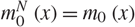 $m_{0}^{N}\left(x\right) =m_{0}\left( x\right)$, where m 0: ℝd → ℝ is a measurable function with 0 ≤ m 0 ≤ M, and the functional
 \begin{equation}b\colon L^{2}(\mathbb{R}^{d})\times L^{2}(\mathbb{R}^{d})\rightarrow L^{\infty }(\mathbb{R}^{d})\end{equation}
is given by (3), where g: ℝ+ × ℝ+ × ℝ+ → ℝ, g = g(r, u, m), is differentiable, bounded with bounded derivatives, and satisfies
 \begin{equation}\label{hyp:g} |g(r,u,m)|+|\nabla g(r,u,m)|\leq C\exp(\!-r) \end{equation}
for some constant C > 0 (where ∇g denotes the gradient in all variables). It follows that, for every pair of measurable functions u(x) and m(x), the aggregation force is bounded:
 \begin{equation}\label{bounded b} |b(u,m)(x)|\leq\int_{\mathbb{R}^{d}}\left\vert g(|y-x|,u(\kern1pt y),m(\kern1pt y))\right\vert {\rm d} y\leq C\int_{\mathbb{R}^{d}}{\rm e}^{-|x-y|} {\rm d} y\colon = C^{\prime}<\infty. \end{equation}
We also have
 \begin{equation}\label{lip 1 b} |b(u,m)(x)-b(u^{\prime},m^{\prime})(x)|\leq C\int_{\mathbb{R}^{d} }{\rm e}^{-|x-y|}( \vert u\left( y\right) -u^{\prime}\left( y\right) \vert +\vert m\left( y\right) -m^{\prime}\left( y\right) \vert ) {\rm d} y, \end{equation}
and, regarding the derivative, due to the condition on the gradient of g,
 \begin{align} |\nabla_{x} b(u,m)(x)|&\leq\bigg| \int_{\mathbb{R}^{d}}\nabla_x\left(\frac{y-x}{|y-x|} g(|y-x|,u(\kern1pt y),m(\kern1pt y))\right){\rm d} y\bigg| \\ &\leq |g(0,u(x),m(x))|+\bigg|\int_{\mathbb{R}^{d}}\frac{y-x}{|y-x|} \nabla_x\left(g(|y-x|,u(\kern1pt y),m(\kern1pt y))\right){\rm d} y\bigg| \\ &\leq C_1+\int_{\mathbb{R}^d}|\partial_r g(|y-x|,u(\kern1pt y),m(\kern1pt y))|{\rm d} y \\ &\leq C_1+C_2.\label{lip 2 b} \end{align}
Under these assumptions, existence and uniqueness of a solution, for finite N, of system (1) can be proved by classical methods. Let us explain some details. Denote by C(L 2), C +(L 2), and C 0,M(L 2) the spaces
 \begin{gather*} C( L^{2}) \colon = C([0,T],L^{2}(\mathbb{R}^{d})), \\ C_{+}( L^{2}) \colon = \{ u\in C( L^{2}) \colon u_{t}\geq0\text{ for all }t\in[ 0,T] \}, \\ C_{0,M}( L^{2}) =\{ m\in C( L^{2}) \colon 0\leq m_{t}\leq M\text{ for all }t\in[ 0,T] \}. \end{gather*}
We say that a random field  $m_{t}^{N}\left( x\right) $, t ∈ [0, T], x ∈ ℝd, defined on
 $\left( \Omega,\; {\mathcal F},\; {{\mathcal F}_{t}},\; {\mathbb P}\right)$, is adapted of class C 0,M(L 2) if, P-a.s., the functions
 $\left( t,x\right) \mapsto m_{t}^{N}\left( x\right) $ belong to C 0,M(L 2) and, for every t ∈ [0, T], the function
 $\left( x,\omega\right) \mapsto m_{t}^{N}\left( x,\omega\right) $ is (
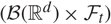 $(\mathcal{B}(\mathbb{R}^{d}) \times\mathcal{F}_{t})$)-measurable. We say that (X 1,N, …, X N,N, m N) is a strong solution of system (1) if
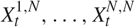 $X_{t}^{1,N},\ldots,X_{t}^{N,N}$ are continuous, adapted processes on
 $\left( \Omega,\; {\mathcal F},\; {{\mathcal F}_{t}},\; {\mathbb P}\right),\;\;m_{t}^{N}\left( x\right) $ is adapted of class C 0,M(L 2), all defined on
 $\left(\Omega,\;{\mathcal F},\; {{\mathcal F}_{t}},\;{\mathbb P}\right)$, and identities (1a)–(1b) hold, with the equations understood integrated in time. We say that pathwise uniqueness holds if two such solutions are indistinguishable processes.
Proposition 1. Given any positive integer N and any function m 0 ∈ L 2(ℝd) such that 0 ≤ m 0 ≤ M, there exists a strong solution of system (1) and pathwise uniqueness holds.
Proof. The proof is classical, we explain only the idea. Given an integer ζ ≥ 1, uN and a.e. x ∈ ℝd, the solution of (1b) is global, unique, and explicit:
 \begin{gather*} m_{t}^{N}(x)=F_{\zeta}\bigg( m_{0}(x),\int_{0}^{t}u_{s}^{N}(x){\rm d} s\bigg), \qquad F_{\zeta}\left( a,b\right) =a\widetilde{F}_{\zeta}\left( a,b\right)\!, \\ \widetilde{F}_{\zeta}\left( a,b\right) = \begin{cases} \exp\left( -\lambda b\right) & \text{if }\zeta=1, \\ \frac{1}{[ a^{\zeta-1}(\zeta-1)\lambda b+1] ^{{1}/{(\zeta-1)}} } & \text{if }\zeta\geq2\text{.} \end{cases} \end{gather*}
The function  $\widetilde{F}_{\zeta}\colon \left[ 0,M\right] \times\lbrack 0,\infty)\rightarrow\mathbb{R}$ is bounded and the function Fζ : [0, M] × [0, ∞) → ℝ is Lipschitz continuous, with at most linear growth in a, uniformly in b. Then we may consider the system of integral equations
 \begin{equation}\label{reduced system} X_{t}^{i,N}=X_{0}^{i}+\int_{0}^{t}b\bigg(u_{s}^{N},F_{\zeta}\bigg( m_{0} (\cdot),\int_{0}^{s}u_{r}^{N}(\cdot){\rm d} r\bigg)\!\bigg)(X_{s}^{i,N}){\rm d} s+\sqrt{2} B_{t}^{i},\qquad i=1,\dots,N, \end{equation}
as a closed system, with only the variables 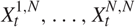 $X_{t}^{1,N},\ldots,X_{t}^{N,N}$. It is a path-dependent equation: the past appears in the drift; but this does not change the way the contraction principle applies. We can check that strong existence and pathwise uniqueness for the original system in the variables (X 1,N, …, X N,N, m N) is equivalent to strong existence and pathwise uniqueness for this reduced path-dependent system in the variables (X 1,N, …, X N,N) only; property mN ∈ C 0,M(L 2) is deduced from the explicit formula. Let us now prove existence and uniqueness for (8). Thanks to property (7), the drift of (8) is globally Lipschitz continuous. We define the family of maps Ji as
 \begin{gather*} J^i\colon E\to \mathbb{R}, \\ J^i(Y)\colon = X_{0}^{i}+\int_{0}^{t}b\bigg(u_{s}^{N},F_{\zeta}\bigg( m_{0} (\cdot),\int_{0}^{s}u_{r}^{N}(\cdot){\rm d} r\bigg)\!\bigg)(Y){\rm d} s+\sqrt{2} B_{t}^{i}, \qquad i=1,\dots,N, \end{gather*}
where  $E=L^2_{\mathcal{F}}(\Omega, C([0,T'],\mathbb{R}^d))$, with T ′ < T. Then with classical computation, we find that Ji is a contraction on the space E,
 \begin{equation}||J^i(Y)-J^i(Y')||_E\leq CT'||Y-Y'||_E,\end{equation}
choosing CT ′ < 1. Hence, local existence and uniqueness of strong solutions is proved. Iterating this argument we can obtain the global existence result, because the amplitude of the interval of iteration depends only on CT ′, namely, it is fixed for each iteration.
Remark 1. Existence and uniqueness of solution of system (1) could be obtained following another approach. With less effort, it could be possible to obtain just weak existence and uniqueness in law for system (1): the method of creating a weak solution to SDEs is transformation of drift via Girsanov’s theorem; see [Reference Karatzas and Shreve6]. With the drift b bounded, see condition (5), hypotheses of Proposition 3.6 and Proposition 3.10 of [Reference Karatzas and Shreve6] are verified, and existence and uniqueness of the system is obtained. Then  $X^{i,N}_t$ is a solution of (1a). Thus,
 $m^N_t$ also exists, is unique, and explicit. This kind of existence would be enough for the purpose of the paper, but we still decide to emphasize in Proposition 1 that a stronger result is attainable.
2.2. Main results
Once the indentity in Lemma 3 below for the empirical measure is proved, it is natural to conjecture that the limit of the pair 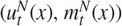 ${( u_{t}^{N}(x) ,m_{t}^{N}(x))}$ solves system (2) with initial condition (u 0, m 0), where u 0 is the density of the random variables (RVs)
 $X_{0}^{i}$ and m 0 is the limit of
 $m_{0}^{N}$. We interpret the first equation of this system in the so called mild form and the second equation in integral form. Concerning the initial conditions, we make a choice of simplicity. We assume that u 0 : ℝd → ℝ (the initial distribution of individuals) is a probability density of class C 1 with compact support, see Lemma 6. We assume that m 0 : ℝd → ℝ is of class L 2(ℝd) and that 0 ≤ m 0 ≤ M.
Definition 1. By a mild solution of system (2) we mean a pair (u, m) belonging to C +(L 2) × C 0,M(L 2) such that
 \begin{gather*} u_{t}(x)={\rm e}^{t\Delta}u_{0}+\int_{0}^{t}\nabla \cdot {\rm e}^{(t-s)\Delta} (u_{s}b(u_{s},m_{s})){\rm d} s, \\ m_{t}(x)=m_{0}(x)-\int_{0}^{t}\lambda u_{s}(x)m_{s}^{\zeta}(x){\rm d} s. \end{gather*}
Here etA denotes the heat semigroup, more precisely defined in Section 2.3. Note that the L 2(ℝd)-norm of usb(us, ms) is bounded, since b is bounded and u ∈ C(L 2). Hence, ∇ · e(t−s)Δ (usb(us, ms)) is integrable by property (3). Convergence of the particles system is proved only locally in space; hence, we introduce the space
 \begin{equation}C( L_{\rm loc}^{2}) \colon = C([0,T],L_{\rm loc}^{2}(\mathbb{R}^{d})),\end{equation}
where the topology on  $L_{\rm loc}^{2}(\mathbb{R}^{d})$ is given by the metric
 \begin{equation}d_{L_{\rm loc}^{2}}\left(\,f,g\right) =\sum_{n=1}^{\infty}2^{-n}(\!\left\|\,f-g\right\| _{L^{2}\left( B\left( 0,n\right) \right) }
\wedge1).\end{equation}
Theorem 1. System (2) has one and only one mild solution (u, m) in C +(L 2) × C 0,M(L 2), and the pair (uN, mN) converges to (u, m) in  $C( L_{\rm loc}^{2}) \times C(L_{\rm loc}^{2}) $, in probability.
2.3. Some useful properties of the analytic semigroup
We denote by Wα, 2(ℝd) the fractional Sobolev space, which is a Banach space with the norm
 \|\begin{equation}f\|_{W^{\alpha,2}(\mathbb{R}^d)}= \|\,f\|_{L^2(\mathbb{R}^d)}+[\,f]_{\alpha,2,\mathbb{R}^d},\end{equation}
where
 \begin{align*} [\,f]_{\alpha,2,\mathbb{R}^d}=\int_{\mathbb{R}^d} \int_{\mathbb{R}^d} \frac{|\,f(x)-f(\kern1pt y)|^2}{|x-y|^{2\alpha+d}}{\rm d} x {\rm d} y. \end{align*}
Or, equivalently,
 \begin{align*} ||u^N_0||_{W^{\alpha,2}}=\| u_{0}^{N}\| _{L^{2}( \mathbb{R}^{d}) } + \| ({-}\Delta) ^{\alpha}u_{0}^{N}\| _{L^{2}( \mathbb{R} ^{d})}, \end{align*}
where the fractional Laplacian can be characterized by the following lemma.
Lemma 1. Let s ∈ (0, 1). Then there exists a constant C (s, d) such that
 \begin{equation}\left( -\Delta\right) ^{s}f\left( x\right) =C\left( s,d\right) \int_{\mathbb{R}^{d}}\frac{f\left( x+y\right) +f\left( x-y\right) -2f\left( x\right) }{\left\vert y\right\vert ^{d+2s}} {\rm d} y, \qquad x\in\mathbb{R}^{d},\end{equation}
for every compact support twice differentiable function f.
Note that boundedness of f guarantees integrability at infinity, while twice differentiability implies that the numerator is, for small |y|, infinitesimal of order two, which compensates the singularity of the denominator. Another very useful property on the fractional Laplacian is that it is a local operator, namely, it preserves the compact support of functions.
Let us recall some well-known properties of analytical semigroups. The family of operators
 \begin{equation}( {\rm e}^{tA}f) \left( x\right) \colon = \int_{\mathbb{R}^{d}}\frac {1}{(2\pi \sigma^2t)^{d/2}}{\rm e}^{-{|x-y|^{2}}/{2\sigma^2t}}f(\kern1pt y) {\rm d} y \quad {{\rm for}\,\, t \geq 0}\end{equation}
defines an analytic semigroup (the heat semigroup) on the space Wα, 2(ℝd) for every α ≥ 0. The infinitesimal generator in L 2(ℝd) is the operator A: D(A) ⊂ L 2(ℝd) → L 2(ℝd), D(A) = W 2,2(ℝd), given by 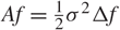 $Af=\tfrac12{\sigma^2}\Delta f$. It is possible to define the fractional power of the operator (I – A)δ for δ ∈ ℝ and a well-known fact is the equivalence of norms:
 \begin{align}\label{prop1_semigroup} \| (I-A)^{\delta/2}f\| _{L^{2}}\sim\|\,f\| _{W^{\delta,2}}.\end{align}
Another property, often used in the sequel, is that, for every δ, T > 0, there is a constant Cδ,T such that, for t ∈ (0, T],
 \begin{align}\label{prop2_semigroup} \| (I-A)^{\delta}{\rm e}^{tA}\| _{L^{2}\rightarrow L^{2}}\leq\frac{C_{\delta,T} }{t^{\delta}}.\end{align}
Finally, we remark that the operator ∇(I − A)−1/2 is bounded in L 2,
 \begin{align}\label{prop3_semigroup} \| \nabla(I-A)^{-1/2}\| _{L^{2}\rightarrow L^{2}}\leq C, \end{align}
where, here and below, we continue to simply write L 2 when the functions are also vector valued, as in the case of ∇(I − A)−1/2f.
It will be useful to know the following result on the improvement of regularity.
Lemma 2. If u ∈ Lp(0, T; L 2(ℝd)) for some p > 2 and satisfies
 \begin{equation}u_{t}(x)={\rm e}^{tA}u_{0}+\int_{0}^{t}\nabla \cdot {\rm e}^{(t-s)A}(u_{s} b_{s}) {\rm d} s\end{equation}
for some bounded measurable function b, then u ∈ C([0, T], L 2(ℝd)).
Proof. The product ub is in Lp(0, T; L 2(ℝd)). Using the bound
 \begin{equation}\| \nabla\cdot {\rm e}^{(t-s)A}\| _{L^{2}\rightarrow L^{2}}=\| \nabla\cdot (I-A)^{-1/2}(I-A)^{1/2}{\rm e}^{(t-s)A}\| _{L^{2}\rightarrow L^{2}} \leq\frac{C}{\left( t-s\right) ^{1/2}},\end{equation}
we deduce that  $t\mapsto\int_{0}^{t}\nabla\cdot {\rm e}^{(t-s)A}(u_{s}b_{s}) {\rm d} s$ is of class C([0, T], L 2(ℝd)); the same is true for t ↦ etAu 0 because u ∈ L 2(ℝd) as a byproduct of our assumptions. Hence, u ∈ C([0, T], L 2(ℝd)).
2.4. Preliminary results
Lemma 3. For every φ ∈ C 2([0, T] × ℝd),  $S_{t} ^{N}$ satisfies the identity
 \begin{align*} \langle S_{t}^{N},\phi_{t}\rangle -\langle S_{0}^{N},\phi _{0}\rangle & = \int_{0}^{t}\bigg\langle S_{s}^{N},\frac{\partial \phi_{s}}{\partial s}\bigg\rangle {\rm d} s+ \frac{\sigma^2}{2}\int_{0}^{t}\langle S_{s} ^{N},\Delta\phi_{s}\rangle {\rm d} s \\ & +\int_{0}^{t}\langle S_{s}^{N},\nabla\phi_{s} b(u_{s}^{N} ,m_{s}^{N})\rangle {\rm d} s+M_{t}^{N,\phi}, \end{align*}
where
 \begin{equation}M_{t}^{N,\phi}=\frac{\sigma}{N}\sum_{i=1}^{N}\int_{0}^{t}\nabla\phi (X_{s}^{i,N}) \cdot {\rm d} B_{s}^{i}.\end{equation}
In particular, choosing φ (·) = φx (·) = WN(· −x) for x ∈ ℝd, we obtain
 \begin{equation}u_{t}^{N}(x)-u_{0}^{N}(x)=\frac{\sigma^2}{2}\int_{0}^{t}\Delta u_{s}^{N}(x){\rm d} s+\int_{0}^{t}\mathrm{div}(W_{N}\ast( b(u_{s}^{N},m_{s}^{N})S_{s}^{N}))(x){\rm d} s+M_{t}^{N}\left( x\right),\end{equation}
where
 \begin{equation}M_{t}^{N}\left( x\right) =\frac{\sigma}{N}\sum_{i=1}^{N}\int_{0}^{t}\nabla W_{N}(x-X_{s}^{i,N}) \cdot {\rm d} B_{s}^{i}.\end{equation}
Proof. The proof follows by Itô’s formula and the Gauss Green formula.
Concerning the family of mollifiers, we have the following useful result, whose proof is an elementary computation; see, for instance, [Reference Flandoli, Leimbach and Olivera5].
Lemma 4. Recall that WN(x) = NβW(Nβ/dx). Then
 \begin{equation}\| W_{N}\| _{L^{2}}^{2}\leq CN^{\beta}, \qquad \| W_{N}\| _{W^{\gamma,2}}^{2}\leq CN^{\gamma^{\ast}},\end{equation}
with γ* = β(2γ + d)/d.
We shall also use the following tightness result.
Lemma 5. Let X 1 and X 2 be two metric spaces with their Borel σ-fields σ-fields  $\mathcal{B}_{1}$ and
 $\mathcal{B}_{1}$, and let φ : X 1 → X 2 be a continuous function. Let
 $\mathcal{G}_{1}$ be a family of probability measures on
 $\left( X_{1},\mathcal{B}_{1}\right) $. Denote by
 $\mathcal{G}_{2}$ the family of probability measures on
 $\left( X_{2},\mathcal{B}_{2}\right) $ obtained as image laws of the measures in
 $\mathcal{G}_{1}$ under the map φ. If
 $\mathcal{G}_{1}$ is tight then
 $\mathcal{G}_{2}$ is tight.
Proof. Given ε > 0, let  $K_{1}^{\varepsilon }\subset X_{1}$ be a compact set such that
 $\mu( K_{1}^{\varepsilon }) >1-\varepsilon $ for every
 $\mu \in\mathcal{G}_{1}$. Set
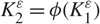 $K_{2}^{\varepsilon }=\phi( K_{1}^{\varepsilon }) $; it is a compact set of X 2 and, for every
 $\nu\in \mathcal{G}_{2}$, with μ a measure in
 $\mathcal{G}_{1}$ such that ν is the image of μ under φ, we have
 \begin{equation}v(K_2^\varepsilon ) = \mu (K_1^\varepsilon ) > 1 - \varepsilon.\end{equation}
This proves tightness of  $\mathcal{G}_{2}$.
Regarding the initial condition, we state the following result, that will be useful in the proof of tightness.
Lemma 6. Assume that  $X^i_0, i = 1,\ldots,N$, are independent, identically distributed RVs with common probability density u 0 ∈ C 2(ℝd). Then, on
 $u^N_0$, defined as
 $u^N_0(x)=(W^N\ast u_0)(x)$, we obtain the uniform bounds
 \begin{equation}\mathbb{E}[ \|u^N_0\|^p_{W^{\alpha,2}}] \leq C_{u_0,\alpha,p} \quad {{for}\,\, p \gt 1},\end{equation}
where C is a constant depending on p and α.
Proof. By the definition of the norm in the fractional Sobolev space, we need to estimate uniformly in N:
 \begin{align} \mathbb{E}[ \|u^N_0\|^p_{W^{\alpha,2}}] =\mathbb{E}[ \| u_{0}^{N}\| _{L^{2}( \mathbb{R}^{d}) }^{p}] +\mathbb{E}[ \| ({-}\Delta) ^{\alpha}u_{0}^{N}\| _{L^{2}( \mathbb{R} ^{d})}^{p}]. \end{align}
We recall that u 0 is compactly supported and, moreover, that the fractional Laplacian is a local operator, namely, it preserves the compactness properties of functions. Then, for p ≥ 2,
 \begin{gather*} \| u_{0}^{N}\| _{L^{2}\left( \mathbb{R}^{d}\right) } ^{p}\leq\int_{\mathcal{B}_1}\vert u_{0}^{N}( x)\vert ^{p} {\rm d} x, \\ \| ({-}\Delta) ^{\alpha}u_{0}^{N}\| _{L^{2}\left( \mathbb{R}^{d}\right) }^{p}\leq \int_{\mathcal{B}_1}\vert \left( -\Delta\right) ^{\alpha}u_{0}^{N}(x) \vert ^{p} {\rm d} x, \end{gather*}
where  $\mathcal{B}_1$ and
 $\mathcal{B}_2$ are respectively compact supports of
 $u^N_0$ and
 $\left( -\Delta\right) ^{\alpha}u_{0}^{N}.$. Assuming that
 \begin{equation}Y^{i}=Y^{i}( x) =W_{N}( x-X_{0}^{i}), \qquad \widetilde{Y}^{i}=\widetilde{Y}^{i}( x) =({-}\Delta) ^{\alpha}W_{N}( x-X_{0}^{i}),\end{equation}
we can write the right-hand side (RHS) estimates of (12) as follows:
 \begin{equation}\text{RHS of (12)} \leq \mathbb{E}\bigg[ \int_{\mathcal{B}_1}\bigg\vert \frac{1} {N}\sum_{i=1}^{N}Y^{i}( x) \bigg\vert ^{p} {\rm d} x\bigg] +\mathbb{E}\bigg[ \int_{\mathcal{B}_2}\bigg\vert \frac{1} {N}\sum_{i=1}^{N}\widetilde{Y}^{i}( x) \bigg\vert ^{p} {\rm d} x\bigg].\end{equation}
Then we need to estimate
 \begin{align*}\label{prove} \mathbb{E}\bigg[ \bigg\vert \frac{1}{N}\sum_{i=1}^{N}Y^{i}( x) \bigg\vert ^{p}\bigg] +\mathbb{E}\bigg[ \bigg\vert \frac{1}{N}\sum _{i=1}^{N}\widetilde{Y}^{i}( x) \bigg\vert ^{p}\bigg]. \end{align*}
With Yi ≥ 0 on the first summand, we have
 \begin{align*} \mathbb{E}\bigg[ \bigg\vert \frac{1}{N}\sum_{i=1}^{N}Y^{i}\bigg\vert ^{p}\bigg] &=\int_{0}^{\infty}\mathbb{P}\bigg( \bigg( \frac{1}{N}\sum_{i=1} ^{N}Y^{i}\bigg) ^{p}>t\bigg) {\rm d} t \\ &=\int_{0}^{\infty}\mathbb{P}\bigg( \frac{1}{N} \sum_{i=1}^{N}Y^{i}>t^{1/p}\bigg) {\rm d} t \\ &=\int_{0}^{\infty}\mathbb{P}\bigg( \exp\bigg( \frac{1}{N}\sum_{i=1}^{N} Y^{i}\bigg) >\exp( t^{1/p}) \bigg) {\rm d} t \\ &\leq\int_{0}^{\infty}\exp( -t^{1/p}) \mathbb{E}\bigg[ \exp\biggl({\biggl(\frac{1}{N}\biggr)\sum_{i=1}^{N}Y^{i}}\biggr)\bigg] {\rm d} t \\ &={\rm e}^{N\log\mathbb{E}[ {\rm e}^{{Y}/{N}}] }\int_{0}^{\infty} \exp( -t^{1/p}) {\rm d} t, \end{align*}
where Y has the same law as Yi. Note that the equality
 \begin{equation}\mathbb{E}\bigg[\exp\bigg({\bigg(\frac{1}{N}\bigg)\sum_{i=1}^{N}Y^{i}}\bigg)\bigg]= {\rm e}^{N\log\mathbb{E}[ {\rm e}^{{Y}/{N}}] }\end{equation}
follows easily from the fact that the Yi are independent and identically distributed (i.i.d.). Because Ỹi ≥ 0 also, the same result holds for the second term. Then
 \begin{align*} &\mathbb{E}\bigg[ \bigg\vert \frac{1}{N}\sum_{i=1}^{N}Y^{i}( x) \bigg\vert ^{p}\bigg] +\mathbb{E}\bigg[ \bigg\vert \frac{1}{N}\sum _{i=1}^{N}\widetilde{Y}^{i}( x) \bigg\vert ^{p}\bigg] \\ &\qquad\leq({\rm e}^{N\log\mathbb{E}[ {\rm e}^{{Y}/{N}}] }+{\rm e}^{N\log\mathbb{E}[ {\rm e}^{{\tilde{Y}}/{N}}] })\int_{0}^{\infty} \exp( -t^{1/p}) {\rm d} t. \end{align*}
We know estimate the first term (the same result will hold for the second term). We recall the basic inequalities log (1 + x) ≤ x and ex − 1 ≤ xex for x ≥ 0. Then
 \begin{align*}\log\mathbb{E}[ {\rm e}^{{Y( x) }/{N}}] & =\log(1+\mathbb{E}[ {\rm e}^{{Y( x) }/{N}}-1] )\\& \leq\mathbb{E}[ {\rm e}^{{Y( x)}/{N}}-1]\\& \leq\mathbb{E}\Big[ \frac{Y\left( x\right) }{N}{\rm e}^{{Y\left( x\right)}/{N}}\Big].\end{align*}
We have to estimate
 \begin{equation}\mathbb{E}[ Y( x){\rm e}^{{Y( x) }/{N}}]\quad\textrm{and}\quad \mathbb{E}[ \tilde{Y}( x) {\rm e}^{{\tilde{Y}( x) }/{N}}].\end{equation}
Recalling the definition of Yi,
 \begin{equation}\frac{Y\left( x\right) }{N}=N^{-1}W_{N}\left( x-X_{0}\right) =N^{\beta -1}W( N^{\beta/d}( x-X_{0})) \leq C.\end{equation}
With W bounded, Y(x)/N is bounded. Now we just need to estimate
 \begin{equation}\mathbb{E}[Y(x)]=(W^N\ast u_0)(x).\end{equation}
The last term is bounded because u 0 is. Let us analyze the second term, which is a bit more delicate. By the definition of Ỹi,
 \begin{equation}\frac{\widetilde{Y}\left( x\right) }{N}=N^{-1}\left( -\Delta\right) ^{\alpha}W_{N}\left( x-X_{0}\right) \leq CN^{-1+\beta}N^{2\alpha\beta/d}.\end{equation}
Choose an α small enough that the term Ỹ (x)/N is bounded. At the end we need to prove a uniform estimate on 𝔼[Ỹ(x)]. We have
 \begin{align*} \mathbb{E}[ \widetilde{Y}( x) ] & =\mathbb{E} [ ({-}\Delta) ^{\alpha}W_{N}( x-X_{0}) ] \\ &=\int[ ({-}\Delta) ^{\alpha}W_{N}] ( x-x_{0}) u_{0}( x_{0})\ {\rm d} x_{0} \\ & =-\int({-}\Delta) ^{\alpha }W_{N}( x_{0}^{\prime}) u_{0}( x-x_{0}^{\prime})\ {\rm d} x_{0}^{\prime} \quad({x_{0}^{\prime}=x-x_{0}}) \\ & =-\langle ({-}\Delta) ^{\alpha}W_{N},u_{0}( x-\cdot) \rangle _{L^{2}} \\ & =-\langle W_{N},({-}\Delta) ^{\alpha}u_{0}( x-\cdot) \rangle _{L^{2}} \\ & =-\int W_{N}( x_{0}^{\prime}) [ ({-}\Delta) ^{\alpha}u_{0}] ( x-x_{0}^{\prime})\ {\rm d} x_{0}^{\prime} \\ & =[ W_{N}\ast( ( -\Delta) ^{\alpha}u_{0}) ]\, ( x). \end{align*}
With (−Δ)α u 0 compactly supported and continuous, WN * ((−Δ)α u 0) is also uniformly bounded. In summary,
 \begin{align*} \mathbb{E}[ \|u^N_0\|^p_{W^{\alpha,2}}] \leq C_{\mathcal{B}_1,\mathcal{B}_2,u_0,\alpha,p}. \end{align*}
3. Tightness
3.1. Compactness of function spaces
We use Corollary 9 of [Reference Simon12], using as far as possible the notation of that paper, for ease of reference. Given a ball BR := B (0, R) in ℝd, letting α > ε > 0, consider the spaces
 \begin{equation}X=W^{\alpha,2}\left( B_{R}\right)\!,\qquad B=W^{\alpha-\varepsilon ,2}\left( B_{R}\right)\!,\qquad Y=W^{-2,2}\left( B_{R}\right).\end{equation}
We have
 \begin{equation}X\subset B\subset Y\end{equation}
with compact dense embeddings. Moreover, we have the interpolation inequality (see Theorem 6.4.5 of [Reference Bergh and Löfström2])
 \begin{equation}\left\|\,f\right\| _{B}\leq C_{R}\left\|\,f\right\| _{X}^{1- \theta }\left\|\,f\right\| _{Y}^{\theta}\end{equation}
for all f ∈ X, with
 \begin{equation}\theta=\frac{\varepsilon }{2+\alpha}.\end{equation}
These are the preliminary assumptions of Corollary 9 of [Reference Simon12]. The corollary states that the embedding of
 \begin{equation}\mathcal{W}_{R}\colon = L^{r_{0}}\left( 0,T;\ X\right) \cap W^{s_{1},r_{1}} \left( 0,T;\ Y\right)\end{equation}
is relatively compact in C ([0, T]; B) if s 1r 1 > 1 and r 0 is large enough that sθ > 1/rθ, where (always following the notation of [Reference Simon12]) sθ = θs 1 and 1/rθ = (1 − θ)/r 0 + θ/r 1. Below we shall choose, for instance,  $s_{1}=\frac{1}{3}$ (any number smaller than
 $\frac{1}{2}$) and r 1 = 4, so s 1r 1 > 1 is fulfilled. Then we need
 \begin{equation}\frac{\theta}{3}>\frac{1-\theta}{r_{0}}+\frac{\theta}{4}.\end{equation}
The logical sequence of our choices is as follows. Given β ∈ (0, 1) (consider β close to 1, which is the most difficult choice), we shall choose α > 0 small enough to satisfy a condition related to β which appears in the proof of Lemma 7 below (when β is close to 1, we have to choose small α). Given this small α, we choose ε ∈ (0, α) and then θ = ε/(2 + α) is determined, typically very small. Now, we choose r 0 large enough that θ/3 > (1 − θ)/r 0 + θ/4. Summarising, we choose (α, s 1, r 1, r 0, ε), in the following way:
• α is determined by β;
• (s 1, r 1) is determined (almost) a priori (in the proof of Proposition 2 below s 1r 1 − r 1/2 < 0);
• r 0 is chosen large enough that θs 1 > (1 − θ)/r 0 + θ/r 1;
• ε < α arbitrarily small.
The final step consists in taking ℝd instead of BR. We denote by  $W_{\rm loc}^{\alpha,2}( \mathbb{R}^{d}) $ the space of functions f ∈ ∩R>0 Wα, 2(BR) and we endow this space with the metric
 \begin{equation}d_{W_{\rm loc}^{\alpha,2}}\left( f,g\right) =\sum_{n=1}^{\infty}2^{-n} ( \|\,f-g\| _{W^{\alpha,2}( B_{n}) }\wedge1).\end{equation}
Under the same conditions on the indexes,
 \begin{equation}\mathcal{W}\colon = L^{r_{0}}( 0,T;\ W^{\alpha,2}( \mathbb{R}^{d})) \cap W^{s_{1},r_{1}}( 0,T;\ W^{-2,2}( \mathbb{R} ^{d}) )\end{equation}
is compactly embedded into  $C( [ 0,T] ;\ W_{\rm loc} ^{\alpha-\varepsilon ,2}( \mathbb{R}^{d}) ) $.
3.2. Main estimate on the empirical density uN
Before examining in detail the derivation of the main estimates for the empirical density, we state the mild formulation for  $u_{t}^{N}$ (see Lemma 3 for the identity for
 $u_{t}^{N}$):
 \begin{equation}u_{t}^{N}={\rm e}^{tA}u_{0}^{N}+\int_{0}^{t}{\rm e}^{(t-s)A}\mathrm{div}(W_{N} \ast( b(u_{s}^{N},m_{s}^{N} )S_{s}^{N}) )(x){\rm d} s+\int _{0}^{t}{\rm e}^{(t-s)A}{\rm d} M_{s}^{N}.\end{equation}
Lemma 7. Given β ∈ (0, 1), there exists α > 0 small enough such that the following assertion holds: for every p > 1, there is a constant Cp > 0 such that
 \begin{equation}\sup_{t\in[ 0,T] }\mathbb{E}[ \| u_{t} ^{N}\| _{W^{\alpha,2}(\mathbb{R}^{d})}^{p}] \leq C_{p}\end{equation}
independently of N.
Proof. Step 1: preliminary estimates. We shall use the equivalence between norms (9):
 \begin{equation}\| (I-A)^{\alpha/2}f\| _{L^{2}(\mathbb{R}^{d})}\sim\|\,f\| _{W^{\alpha ,2}(\mathbb{R}^{d})}.\end{equation}
Then, up to a constant, letting  $f_{s}^{N}(x)=\mathrm{div}(W_{N} \ast( b(u_{s}^{N},m_{s}^{N} )S_{s}^{N}))(x)$,
 \begin{align*} \| u_{t}^{N}\| _{W^{\alpha,2}(\mathbb{R}^{d})} & \leq\| (I-A)^{\alpha /2}{\rm e}^{tA}u_{0}^{N}\| _{L^{2}(\mathbb{R}^{d})}+\| (I-A)^{\alpha/2} \int_{0}^{t}{\rm e}^{(t-s)A}f_{s}^{N}{\rm d} s\| _{L^{2}(\mathbb{R}^{d})} \\ & +\| (I-A)^{\alpha/2}\int_{0}^{t}{\rm e}^{(t-s)A}{\rm d} M_{s}^{N} \| _{L^{2}(\mathbb{R}^{d})}. \end{align*}
For the first term, using (10), we prove the estimate
 \begin{align*} \mathbb{E}[ \| (I-A)^{\alpha/2}{\rm e}^{tA}u_{0}^{N}\| _{L^{2} (\mathbb{R}^{d})}^{p}] & \leq\| {\rm e}^{tA}\| _{L^{2}\rightarrow L^{2}}^{p}\mathbb{E}[ \| (I-A)^{\alpha/2}u_{0}^{N}\| _{L^{2}(\mathbb{R}^{d})}^{p}] \\ &\leq C\mathbb{E}[ \| u_{0}^{N}\| _{W^{\alpha,2}(\mathbb{R}^{d})}^{p}]. \end{align*}
The last expected value is bounded by the assumption that u 0 is a C 1 compact support: in this case we can show convergence of the empirical means of the i.i.d. RVs  $X_{0}^{i}$, which implies a uniform in N bound on
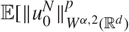 $\mathbb{E}[\| u_{0}^{N}\| _{W^{\alpha,2} (\mathbb{R}^{d})}^{p}] $ for every p (see [Reference Flandoli, Leimbach and Olivera5] for similar results).
For the third term, we use the following fact. For every p > 1, there is a constant Cp > 0 such that, if 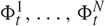 $\Phi_{t}^{1},\ldots,\Phi_{t}^{N}$ are adapted square-integrable processes with values in a Hilbert space H,
 \begin{equation}\mathbb{E}\bigg[ \bigg\| \sum_{i=1}^{N}\int_{0}^{T}\Phi_{t}^{i}{\rm d} B_{t} ^{i}\bigg\| _{H}^{p}\bigg] \leq C_{p}\mathbb{E}\bigg[ \bigg( \sum_{i=1}^{N}\int_{0}^{T}\bigg\| \Phi_{t}^{i}\bigg\| _{H} ^{2}{\rm d} t\bigg) ^{p/2}\bigg].\end{equation}
Therefore,
 \begin{align*} & \mathbb{E}\bigg[ \bigg\| \int_{0}^{t}(I-A)^{\alpha/2} {\rm e}^{(t-s)A}{\rm d} M_{s}^{N}\bigg\| _{L^{2}(\mathbb{R}^{d})}^{p}\bigg] \\ &\qquad =\mathbb{E}\bigg[ \bigg\| \frac{\sigma}{N}\sum_{i=1}^{N}\int_{0} ^{t}(I-A)^{\alpha/2}{\rm e}^{(t-s)A}\nabla W_{N}(\cdot-X_{s}^{i,N} ){\rm d} B_{s}^{i}\bigg\| _{L^{2}(\mathbb{R}^{d})}^{p}\bigg] \\ &\qquad \leq C_{p}\mathbb{E}\bigg[ \bigg( \frac{\sigma^2}{N^{2}} \sum_{i=1}^{N}\int _{0}^{T}\| (I-A)^{\alpha/2}{\rm e}^{(t-s)A}\nabla W_{N} (\cdot-X_{s}^{i,N})\| _{L^{2}(\mathbb{R}^{d})}^{2}{\rm d} s\bigg) ^{p/2}\bigg] \\ &\qquad =C_{p}\mathbb{E}\bigg[ \bigg( \frac{\sigma^2}{N^{2}}\sum_{i=1}^{N} \int_{0} ^{T}\| (I-A)^{\alpha/2} {\rm e}^{(t-s)A}\nabla W_{N}\| _{L^{2}(\mathbb{R}^{d})}^{2}{\rm d} s\bigg) ^{p/2}\bigg] \\ &\qquad =C_{p}\bigg( \frac{\sigma^2}{N}\int_{0}^{T}\| (I-A)^{\alpha /2}{\rm e}^{(t-s)A}\nabla W_{N}\| _{L^{2}(\mathbb{R}^{d})}^{2}{\rm d} s\bigg) ^{p/2}.\end{align*}
Moreover, the gradient commutes with the heat semigroup and the fractional powers of the Laplacian. Hence, using (10) and (11), the integrand can be estimated as
 \begin{align*} & \| (I-A)^{\alpha/2}{\rm e}^{(t-s)A}\nabla W_{N}\| _{L^{2}(\mathbb{R}^{d})}^{2} \\ &\qquad \leq[ \| \nabla(I-A)^{-1/2}\| _{L^{2}\rightarrow L^{2}} \| (I-A)^{{(1-\varepsilon)}/{2}}{\rm e}^{(t-s)A}\| _{L^{2}\rightarrow L^{2} }\| (I-A)^{{(\alpha+\varepsilon)}/{2}}W_{N}\| _{L^{2}(\mathbb{R}^{d} )}] ^{2} \\ &\qquad \leq\frac{c}{(t-s)^{1-\varepsilon }}\| W_{N}\| _{W^{\alpha+\varepsilon ,2} (\mathbb{R}^{d})}^{2}.\end{align*}
From Lemma 4 we obtain
 \begin{equation}\| (I-A)^{\alpha/2}{\rm e}^{(t-s)A}\nabla W_{N}\| _{L^{2}(\mathbb{R}^{d})}^{2}\leq\frac{c}{(t-s)^{1-\varepsilon }}N^{(\alpha +\varepsilon )^{\ast}},\end{equation}
and thus we can estimate the martingale term in the following way:
 \begin{align*} \mathbb{E}\bigg[ \bigg\| \int_{0}^{t}(I-A)^{\alpha/2} {\rm e}^{(t-s)A}{\rm d} M_{s}^{N}\bigg\| _{L^{2}(\mathbb{R}^{d})}^{p}\bigg] & \leq C_{p}\left( \frac{\sigma^2}{N}\int_{0}^{T}\frac{c}{(t-s)^{1-\varepsilon } }N^{(\alpha+\varepsilon )^{\ast}}{\rm d} s\right) ^{p/2} \\ & =C_{p,T}\left( \frac{N^{(\alpha+\varepsilon )^{\ast}}}{N}\right) ^{p/2}. \end{align*}
Choosing α small enough that (α + ε)* ≤ 1, i.e. β ≤ d/(2(α + ε) + d) < 1, we obtain a uniform bound on the martingale term.
Finally, thanks to the boundness on b we obtain the estimate
 \begin{align*} \vert W_{N}\ast( b(u_{t}^{N},m_{t}^{N})S_{t}^{N}) (x) \vert & =\left\vert \int_{\mathbb{R}^{d}}W_{N}\left( x-y\right) b(u_{t}^{N} ,m_{t}^{N})(y) S_{t}^{N}\left( {\rm d}y\right) \right\vert \\ & \leq\int_{\mathbb{R}^{d}}W_{N}\left( x-y\right) \vert b(u_{t} ^{N},m_{t}^{N})(y) \vert S_{t}^{N}\left({\rm d} y\right) \\ & \leq C\int_{\mathbb{R}^{d}}W_{N}\left( x-y\right) S_{t}^{N}\left( {\rm d} y\right) \\ & =Cu_{t}^{N}\left( x\right)\!;\end{align*}
hence,
 \begin{equation}\| W_{N}\ast( b(u_{t}^{N},m_{t}^{N})S_{t}^{N}) \| _{L^{2} (\mathbb{R}^{d})}^{2}\leq C\| u_{t}^{N}\| _{L^{2}(\mathbb{R}^{d})}.\end{equation}
Step 2: estimate in L 2(ℝd). Consider the α = 0 case in the previous computations. We have proved, with the notation H = L 2(ℝd), that
 \begin{equation}\| u_{t}^{N}\| _{L^{p}\left( \Omega;H\right) }\leq C+\left\| \int_{0}^{t}{\rm e}^{(t-s)A}f_{s}^{N}{\rm d} s\right\| _{L^{p}\left( \Omega;H\right) }.\end{equation}
Thus,
 \begin{equation}\| u_{t}^{N}\| _{L^{p}\left( \Omega;H\right) }\leq C+\int_{0}^{t}\| {\rm e}^{(t-s)A}f_{s}^{N}\| _{L^{p}\left( \Omega;H\right) }{\rm d} s.\end{equation}
We have
 \begin{align*} \| {\rm e}^{(t-s)A}f_{s}^{N}\| _{L^{p}( \Omega;H) } & =\mathbb{E}[ \| \nabla\cdot {\rm e}^{(t-s)A}(W_{N} \ast( b(u_{t}^{N},m_{t}^{N})S_{t}^{N}) \| _{L^{2} (\mathbb{R}^{d})}^{p}] ^{1/p}\\& \leq\| \nabla \cdot {\rm e}^{(t-s)A}\| _{L^{2}\rightarrow L^{2}}\mathbb{E}[ \| W_{N}\ast b(u_{t}^{N},m_{t}^{N})S_{t} ^{N}\| _{L^{2}(\mathbb{R}^{d})}^{p}] ^{1/p} \\ & \leq\frac{C}{(t-s)^{{1}/{2}}}\| u_{s}^{N}\| _{L^{p}( \Omega;H) }, \end{align*}
using properties on the analytical semigroup, (10) and (11), and the last bound of step 1. Therefore,
 \begin{equation}\| u_{t}^{N}\| _{L^{p}\left( \Omega;H\right) }\leq C+\int_{0}^{t}\frac{C}{(t-s)^{{1}/{2}}}\| u_{s}^{N}\| _{L^{p}\left( \Omega;H\right) }{\rm d} s.\end{equation}
A generalised form of the Gronwall lemma implies that
 \begin{equation}\sup_{t\in\left[ 0,T\right] }\| u_{t}^{N}\| _{L^{p}\left( \Omega;H\right) }\leq C,\end{equation}
where the constant C depends on p but not on N.
Step 3: estimate in Wα, 2(ℝd). Similarly to the beginning of step 2, we have
 \begin{equation}\| u_{t}^{N}\| _{L^{p}\left( \Omega;\widetilde{H}\right) }\leq C+\int_{0}^{t}\| {\rm e}^{(t-s)A}f_{s}^{N}\| _{L^{p}\left( \Omega;\widetilde{H}\right) }{\rm d} s,\end{equation}
where now H̃ = Wα, 2(ℝd); recalling some properties of the analytical semigroup (see (9),(10), and (11)), we obtain
 \begin{equation}\| {\rm e}^{(t-s)A}f_{s}^{N}\| _{L^{p}\left( \Omega ;\widetilde{H}\right) }\leq\frac{C}{(t-s)^{{(\alpha+1)}/{2}}}\| u_{s}^{N}\| _{L^{p}\left( \Omega;H\right) }.\end{equation}
However, from step 2 we know that  $\| u_{s}^{N}\|_{L^{p}\left( \Omega;H\right) }$ is uniformly bounded; hence, for α < 1, we deduce the claim of the lemma.
3.3. Tightness of ( ${u_{t}^{N}},{m_{t}^{N}}$)

Recall from Section 3.1 that the space there denoted by  $\mathcal{W}$ is compactly embedded in
 $C( [ 0,T] ;W_{\rm loc}^{\alpha-\varepsilon ,2}( \mathbb{R}^{d}) ) $ when
 $s_{1}=\frac{1}{3}$ and r 1 = 4, and when, having chosen α small enough related to the original choice of β such that the result of Lemma 7 holds, we take r 0 large enough.
In order to prove tightness of the family of laws of  $u_{t}^{N}$ in
 $\mathcal{W}$, we have to prove that
 $u_{t}^{N}$ is bounded in probability in Lr 0(0, T;Wα, 2(ℝd)) and in Ws 1,r1(0, T;W −2,2(ℝd)). For the first claim, it is sufficient to prove that
 \begin{equation}\mathbb{E}\int_{0}^{T}\| u_{t}^{N}\| _{W^{\alpha,2}\left( \mathbb{R}^{d}\right) }^{r_{0}}{\rm d} t\leq C,\end{equation}
which is true by Lemma 7 because
 \begin{equation}\mathbb{E}\int_{0}^{T}\| u_{t}^{N}\| _{W^{\alpha,2}( \mathbb{R}^{d}) }^{r_{0}}{\rm d} t=\int_{0}^{T}\mathbb{E}[ \| u_{t}^{N}\| _{W^{\alpha,2}( \mathbb{R}^{d}) }^{r_{0} }] {\rm d} t\leq\sup_{t\in[ 0,T] }\mathbb{E}[ \| u_{t}^{N}\| _{W^{\alpha,2}(\mathbb{R}^{d})}^{r_{0}}].\end{equation}
The second claim is proved in the next proposition.
Proposition 2. The family  $\{u_{t}^{N}\}_{N}$ is bounded in probability in Ws 1,r1(0, T;W −2,2(ℝd)).
Proof. Let us recall that a norm on Ws 1,r1(0, T;W −2,2(ℝd)) is given by the sum
 \begin{equation}\left( \int_{0}^{T}\left\|\,f_{t}\right\| _{W^{-2,2}\left( \mathbb{R}^{d}\right) }^{r_{1}}{\rm d} t\right) ^{1/r_{1}}+ \bigg( \int_{0}^{T} \int_{0}^{T}\frac{\|\,f_{t}-f_{s}\| _{W^{-2,2}( \mathbb{R}^{d}) }^{r_{1}}}{\vert t-s\vert ^{1+s_{1}r_{1}} }{\rm d} t{\rm d} s\bigg) ^{1/r_{1}}.\end{equation}
The property
 \begin{equation}\mathbb{E}\int_{0}^{T}\| u_{t}^{N}\| _{W^{-2,2}\left( \mathbb{R}^{d}\right) }^{r_{1}}{\rm d} t\leq C\end{equation}
is a consequence of Lemma 7 because  $\| u_{t} ^{N}\|_{W^{-2,2}}$ is a weaker norm than
 $\| u_{t} ^{N}\|_{W^{\alpha,2}}$. We have to prove that
 \begin{equation}\mathbb{E}\int_{0}^{T}\int_{0}^{T}\frac{\| u_{t}^{N}-u_{s} ^{N}\| _{W^{-2,2}\left( \mathbb{R}^{d}\right) }^{r_{1}}} {\left\vert t-s\right\vert ^{1+s_{1}r_{1}}}{\rm d} t{\rm d} s\leq C.\end{equation}
Thus, for t > s, we have to estimate
 \begin{equation}\mathbb{E}[ \| u_{t}^{N}-u_{s}^{N}\| _{W^{-2,2}(\mathbb{R}^{d})}^{r_{1} }].\end{equation}
From the equation satisfied by  $u_{t}^{N}$, proved in Lemma 3, and Hölder’s inequality, we have
 \begin{align*} &\mathbb{E}[ \| u_{t}^{N}-u_{s}^{N}\| _{W^{-2,2}(\mathbb{R}^{d})}^{r_{1} }] \\ &\qquad \leq C(t-s)^{r_{1}-1}\mathbb{E}\int_{s}^{t}\| A u_{r} ^{N}\| _{W^{-2,2}(\mathbb{R}^{d})}^{r_{1}}{\rm d} r+C\mathbb{E}[ \| M_{t} ^{N}-M_{s}^{N}\| _{W^{-2,2}(\mathbb{R}^{d})}^{r_{1}}] \\ &\qquad +C(t-s)^{r_{1}-1}\mathbb{E}\int_{s}^{t}\| \text{div}(W_{N}\ast b(u_{r} ^{N},m_{r}^{N})S_{r}^{N})\| _{W^{-2,2}(\mathbb{R}^{d})}^{r_{1}} {\rm d} r. \end{align*}
With A a bounded operator from L 2 to W −2,2, we have
 \begin{equation}C(t-s)^{r_{1}-1}\mathbb{E}\int_{s}^{t}\| A u_{r}^{N}\| _{W^{-2,2} (\mathbb{R}^{d})}^{r_{1}}{\rm d} r\leq C(t-s)^{r_{1}-1}\int_{s}^{t}\mathbb{E}[ \| u_{r}^{N}\| _{L^{2}(\mathbb{R}^{d})}^{r_{1}}] {\rm d} r\leq C(t-s)^{r_{1}}\end{equation}
thanks to the estimate in Lemma 7. Note that the spaces L 2 and W 1,2 are continuously embedded in W −2,2, namely, there exists a constant C > 0 such that ||f||W−2,2 ≤ C ||f||L2 and ||f ||W−2,2 ≤ C ||f||W−1,2. We shall use this in the following computations. We have
 \begin{align*} \| \text{div}(W_{N}\ast b(u_{r}^{N},m_{r}^{N})S_{r}^{N})\| _{W^{-2,2} (\mathbb{R}^{d})} & \leq C\| (W_{N}\ast b(u_{r}^{N},m_{r}^{N})S_{r}^{N}\| _{W^{-1,2} (\mathbb{R}^{d})} \\ & \leq C\| (W_{N}\ast b(u_{r}^{N},m_{r}^{N})S_{r}^{N})\| _{L^{2}(\mathbb{R} ^{d})} \\ & \leq C\| u_{r}^{N}\| _{L^{2}(\mathbb{R}^{d})}, \end{align*}
where the last inequality is similar to that proved in Lemma 7. Hence,
 \begin{align*} & C(t-s)^{r_{1}-1}\mathbb{E}\int_{s}^{t}\| \text{div}(W_{N}\ast b(u_{r} ^{N},m_{r}^{N})S_{r}^{N})\| _{W^{-2,2}(\mathbb{R}^{d})}^{r_{1}}{\rm d} r \\ &\qquad \leq C(t-s)^{r_{1}-1}\int_{s}^{t}\mathbb{E}[ \| u_{r}^{N} \| _{L^{2}(\mathbb{R}^{d})}^{r_{1}}] {\rm d} r \\ &\qquad\leq C(t-s)^{r_{1}},\end{align*}
as above. Therefore, we have proved that
 \begin{equation}\mathbb{E}[ \| u_{t}^{N}-u_{s}^{N}\| _{W^{-2,2}(\mathbb{R}^{d})}^{r_{1} }] \leq C(t-s)^{r_{1}}+C\mathbb{E}[ \| M_{t}^{N}-M_{s} ^{N}\| _{W^{-2,2}(\mathbb{R}^{d})}^{r_{1}}].\end{equation}
Estimating the martingale as in Lemma 7, we have
 \begin{align*} \mathbb{E}\bigg[ \| M_{t}^{N}-M_{s}^{N}\| _{W^{-2,2}(\mathbb{R}^{d})} ^{r_{1}}\bigg] & =\mathbb{E}\bigg[ \bigg\| \frac{\sigma}{N}\sum_{i=1}^{N}\int_{s} ^{t}\nabla W_{N}(\cdot-X_{u}^{i,N}){\rm d} B_{u}^{i}\bigg\| _{W^{-2,2} (\mathbb{R}^{d})}^{r_{1}}\bigg] \\ & \leq C_{r_{1}}\mathbb{E}\bigg[ \bigg( \frac{\sigma^2}{N^{2}}\sum_{i=1}^{N} \int_{s}^{t}\| \nabla W_{N}(\cdot-X_{u}^{i,N})\| _{W^{-2,2}(\mathbb{R}^{d})}^{2}{\rm d} u\bigg) ^{r_{1}/2}\bigg] \\ & \leq C_{r_{1}}^{\prime}\mathbb{E}\bigg[ \bigg( \frac{\sigma^2}{N^{2}}\sum _{i=1}^{N}\int_{s}^{t}\| W_{N}(\cdot-X_{u}^{i,N})\| _{L^{2}(\mathbb{R}^{d})}^{2}{\rm d} u\bigg) ^{r_{1}/2}\bigg] \\ & =C_{r_{1}}^{\prime}\mathbb{E}\bigg[ \bigg( \frac{\sigma^2}{N}\left\| W_{N}\right\| _{L^{2}(\mathbb{R}^{d})}^{2}\bigg) ^{r_{1}/2}\bigg] \\ & \leq C_{r_{1}}^{\prime}\mathbb{E}\bigg[ \bigg( \frac{\sigma^2}{N}N^{\beta }\bigg) ^{r_{1}/2}\bigg] \left( t-s\right) ^{r_{1}/2},\end{align*}
by Lemma 4; hence (being β < 1),
 \begin{equation}\mathbb{E}[ \| M_{t}^{N}-M_{s}^{N}\| _{W^{-2,2}(\mathbb{R}^{d})}^{r_{1} }] \leq C\left( t-s\right) ^{r_{1}/2}.\end{equation}
Summarising,
 \begin{equation}\mathbb{E}[ \| u_{t}^{N}-u_{s}^{N}\| _{W^{-2,2}(\mathbb{R}^{d})}^{r_{1} }] \leq C\left( t-s\right) ^{r_{1}/2}.\end{equation}
It follows that
 \begin{align*} \mathbb{E}\int_{0}^{T}\int_{0}^{T}\frac{\| u_{t}^{N}-u_{s} ^{N}\| _{W^{-2,2}\left( \mathbb{R}^{d}\right) }^{r_{1}}}{\left\vert t-s\right\vert ^{1+s_{1}r_{1}}}{\rm d} t{\rm d} s \leq\mathbb{E}\int_{0}^{T}\int_{0}^{T}\frac{C}{\left\vert t-s\right\vert ^{1+s_{1}r_{1}-{r_{1}}/{2}}}{\rm d} t{\rm d} s, \end{align*}
which is finite if s 1r 1 − r 1/2 < 0; with our choices  $s_{1}=\frac{1}{3}$ and r 1 = 4, such an assertion holds.
Corollary 1. The family  $\{u_{t}^{N}\}_{N}$ is bounded in probability in
 $\mathcal{W}$, and, therefore, the family of laws of
 $\{u_{t}^{N}\}_{N}$ is tight in
 $C( [ 0,T] ;W_{\rm loc}^{\alpha -\varepsilon ,2}( \mathbb{R}^{d})) $. In particular, it is tight in
 $C( L_{\rm loc}^{2}) $. If Qu is any limit measure of this family and u is a RV with law Qu, we also have the property that
 \begin{equation}\mathbb{E}\int_{0}^{T}\left\| u_{t}\right\| _{L^{2}\left( \mathbb{R}^{d}\right) }^{r_{0}}{\rm d} t<\infty,\end{equation}
namely, Qu is supported on Lp(0, T;L 2(ℝd)) for some p > 2. Therefore, if we prove that Qu is supported on mild solutions, by Lemma 2 we deduce that Qu is supported on C(L 2).
Proposition 3. The family of laws of  $\{m_{t}^{N}\}_{N}$ is tight in
 $C( L_{\rm loc}^{2}) $. If Qm is any limit measure of this family and m is a RV with law Qm, we also have the property that
 \begin{equation}\mathbb{E}\int_{0}^{T}\left\| m_{t}\right\| _{L^{2}\left( \mathbb{R}^{d}\right) }^{r_{0}}{\rm d} t<\infty,\end{equation}
namely, Qm is supported on Lp(0, T;L 2(ℝd)) for some p > 2. Therefore, if we prove that Qm is supported on mild solutions, by Lemma 2 we deduce that Qm is supported on C(L 2).
Proof. Let  $C_{+}( L_{\rm loc}^{2})$ be the space of nonnegative functions of class
 $C( L_{\rm loc}^{2})$. Recall the explicit form of the solution of (1b) given in Proposition 1. We want to apply Lemma 5 with
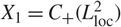 $X_{1} =C_{+}(L_{\rm loc}^{2}) $,
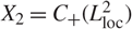 $X_{2}=C_{+}( L_{\rm loc}^{2})$,
 $\mathcal{G}_{1}$ given by the family of laws of
 $\{u_{t}^{N}\}_{N}$,
 $\mathcal{G}_{2}$ given by the family of laws of
 $\{m_{t}^{N}\}_{N}$, and φ given by (for
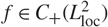 $f\in C_{+}( L_{\rm loc}^{2})$, it is here that we use nonnegativity)
 \begin{equation}\left( \phi f\right) _{t}\left( x\right) \colon = F_{\zeta}\bigg( m_{0} (x),\int_{0}^{t}f_{s}(x){\rm d} s\bigg),\end{equation}
where Fζ (a, b) was introduced in Proposition 1. Tightness of the family  $\mathcal{G}_{1}$ is given by Proposition 2. To prove continuity of φ, we first note that the map
 \begin{equation}f\mapsto\int_{0}^{t}f(s,x){\rm d} s\end{equation}
is continuous from  $C( L_{\rm loc}^{2})$ to
 $C( L_{\rm loc} ^{2})$, and then we compose it with a bounded continuous map.
4. Passage to the limit
Denote by QN the law of (uN, mN) on the space  $C( L_{\rm loc}^{2}) \times C( L_{\rm loc}^{2}) $. We have proved that the family {QN} is tight. Hence, by Prohorov’s theorem, there is a subsequence QNk which converges weakly to some probability measure Q on
 $C( L_{\rm loc}^{2}) \times C( L_{\rm loc}^{2})$. Moreover, from Corollary 1, the marginal Qu on the first component is supported on the space Lp(0, T;L 2(ℝd)) for some p > 2. We first prove that Q is supported on the class of mild solutions of system (2). We then prove that this class has a unique element (u, m); it will follow that the full sequence {QN} converges to δ (u,m) in the weak sense of measures, and that (uN, mN) converges in probability to (u, m) because the limit is deterministic. This will complete the proof of Theorem 1; verification of the properties ut ≥ 0 and 0 ≤ mt ≤ M for every t ∈ [0, T] are done with the same technique as used in the proof of the next proposition, through suitable continuous functionals; we omit the details. The regularity
 $C(L^{2}) \times C( L^{2}) $ of (u, m) comes from Corollary 1 and Proposition 3. In the following proof, we prove that Q is supported on the class of mild solutions of system (2). The proof of the following result is quite classical. It has been widely used in the mean-field theory; see [Reference Sznitman13]. Our case is very close to the mean-field framework, but it cannot be considered a particular case of the known mean-field theories, in particular because of the presence of uN and the dependence of the function g on a density of particles. To prove this step, we adopt the approach of [Reference Kipnis and Landim7, Chapter 4], although presumably it can be proved along several classical lines; see [Reference Sznitman13]. Before going in to the details of the proof, we introduce a family of functionals which characterizes the solution of the system
 \begin{align*} (u,m) & \rightarrow\Psi_{\phi}(u,m)\\ &\colon = \sup_{t\in\left[ 0,T\right] }\bigg\vert \left\langle u_{t}-u_{0},\phi\right\rangle -\frac{\sigma^2} {2}\int_{0} ^{t}\left\langle u_{s},\Delta\phi\right\rangle {\rm d} s-\int_{0}^{t}\left\langle u_{s},b(u_{s},m_{s})\cdot \nabla\phi\right\rangle {\rm d} s\bigg\vert\\ &\hskip2.9pt +\sup_{t\in\left[ 0,T\right] }\bigg\vert \langle m_{t}\left( \cdot\right) -F_{\zeta}\bigg( m_{0}(\!\cdot\!),\int_{0}^{t}u_{s}(\!\cdot\!){\rm d} s\bigg),\phi\rangle\bigg\vert, \end{align*}
where 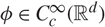 $\phi\in C_{c}^{\infty}(\mathbb{R}^{d})$. On these family we prove a preliminary result to Proposition 4 below.
Lemma 8. Let QNk be the subsequence of measure of QN that converges to Q on  $C( L_{\rm loc}^{2}) \times C( L_{\rm loc}^{2})$. Then
 \begin{equation}\lim_{k\to \infty}Q^{N_{k}}( (u,m)\colon \Psi_{\phi}(u,m)>\delta) =0.\end{equation}
Proof. We have
 \begin{align*} & Q^{N_{k}}( (u,m)\colon \Psi_{\phi}(u,m)>\delta) \\ &\qquad =\mathbb{P}\biggl( \sup_{t\in[ 0,T] }\bigg\vert \langle u_{t}^{N_{k}}-u_{0}^{N_{k}},\phi\rangle -\frac{\sigma^2}{2}\int_{0}^{t}\langle u_{s}^{N_{k}},\Delta\phi\rangle {\rm d} s-\int_{0}^{t}\langle u_{s} ^{N_{k}},b(u_{s}^{N_{k}},m_{s}^{N_{k}})\cdot\nabla\phi\rangle {\rm d} s\bigg\vert\\ &\qquad\quad + \sup_{t\in[ 0,T] }\bigg\vert \langle m_{t}^{N_{k} }( \cdot) -F_{\zeta}\biggl( m_{0}(\cdot),\int_{0}^{t}u_{s} ^{N_{k}}(\cdot){\rm d} s\biggr) ,\phi\rangle\bigg\vert >\delta\biggr) .\end{align*}
The second term of the functional is clearly 0, because of the equation satisfied by  $m_{t}^{N_{k}}$. Using the identity satisfied by
 $u_{t}^{N_{k}}$, we obtain
 \begin{align*} & Q^{N_{k}}( (u,m)\colon \Psi_{\phi}(u,m)>\delta) \\ &\qquad \leq\mathbb{P}\bigg( \sup_{t\in\left[ 0,T\right] }\bigg\vert \bigg\langle \int_{0}^{t}[ W_{N_{k}}\ast(b(u_{s}^{N_{k}},m_{s}^{N_{k}}) S_{s}^{N_{k} })-u_{s}^{N_{k}}b(u_{s}^{N_{k}},m_{s}^{N_{k}})] {\rm d} s,\nabla \phi\bigg\rangle \\ &\qquad\quad+\langle M_{t}^{N_{k}},\phi\rangle \bigg\vert >\delta\bigg) .\end{align*}
Hence, it is sufficient to prove that, for given δ > 0, both the probabilities
 \begin{equation}\mathbb{P}\bigg( \int_{0}^{T}\vert \langle W_{N_{k}}\ast (b(u_{s}^{N_{k}},m_{s}^{N_{k}})S_{s}^{N_{k}})-u_{s}^{N_{k}}b(u_{s}^{N_{k} },m_{s}^{N_{k}}),\nabla\phi\rangle \vert {\rm d} s > \delta \bigg) \end{equation}
and
 \begin{align*} \mathbb{P}\Big( \sup_{t\in[ 0,T] }\vert \langle M_{t}^{N_{k}},\phi\rangle \vert >\delta\Big) \end{align*}
converge to 0 as k → ∞. The first probability is bounded above:
 \begin{equation}{(13)}\leq\mathbb{P}\bigg( C\int_{0}^{T}\| W_{N_{k}}\ast(b(u_{s}^{N_{k} },m_{s}^{N_{k}})S_{s}^{N_{k}})-u_{s}^{N_{k}}b(u_{s}^{N_{k}},m_{s}^{N_{k} })\| _{L^{2}}{\rm d} s>\delta\bigg).\end{equation}
We have
 \begin{align*} & \vert ( W_{N_{k}}\ast(b(u_{s}^{N_{k}},m_{s}^{N_{k}})S_{s} ^{N_{k}})) ( x) -u_{s}^{N_{k}}( x) b(u_{s}^{N_{k}},m_{s}^{N_{k}})( x) \vert \\ &\qquad \leq\int W_{N_{k}}( x-y) \vert b(u_{s}^{N_{k}} ,m_{s}^{N_{k}})( x) -b(u_{s}^{N_{k}},m_{s}^{N_{k}})( y) \vert S_{s}^{N_{k}}( {\rm d} y) \\ &\qquad \leq C^{\prime\prime}\int W_{N_{k}}\left( x-y\right) \left\vert x-y\right\vert S_{s}^{N_{k}}\left( {\rm d} y\right)\quad ({\rm using}\; {\rm property} (7)) \\ &\qquad\leq CN_{k}^{-\beta/d}\int W_{N_{k}}\left( x-y\right) S_{s}^{N_{k}}\left( {\rm d} y\right).\label{neweq2} \end{align*}
Defining WN(x) := NβW(Nβ/dx) and using the property of compact support of W,
 \begin{equation}CN_{k}^{-\beta/d}\int W_{N_{k}}\left( x-y\right) S_{s}^{N_{k}}\left( {\rm d} y\right)=CN_{k}^{-\beta/d}u_{s}^{N_{k}}\left( x\right).\end{equation}
Hence,
 \begin{align*} {(13)} \leq\mathbb{P}\bigg( CN_{k}^{-\beta/d}\int_{0}^{T}\| u_{s}^{N_{k} }\| _{L^{2}}{\rm d} s>\delta\bigg) \leq\frac{CN_{k}^{-\beta/d}}{\delta}\mathbb{E}\int_{0}^{T}\| u_{s}^{N_{k}}\| _{L^{2}}{\rm d} s, \end{align*}
which goes to 0 (recall the bound of Lemma 7).
Finally,
 \begin{align*} \mathbb{P}\Big( \sup_{t\in\left[ 0,T\right] }\vert \langle M_{t}^{N_{k}},\phi\rangle \vert >\delta\Big) & \leq \mathbb{P}\Big( \sup_{t\in\left[ 0,T\right] }\| M_{t}^{N_{k}}\| _{L^{2}}>\delta\Big) \\ & \leq\frac{1}{\delta^{2}}\mathbb{E}\Big[ \sup_{t\in\left[ 0,T\right] }\| M_{t}^{N_{k}}\| _{L^{2}}^{2}\Big] \\ &\leq\frac{C_{T} }{\delta^{2}}\frac{N_k^{\varepsilon \ast}}{N_k}, \end{align*}
as in the proof of Lemma 7 (with α = 0, p = 2, without semigroup, and using Doob’s inequality), which goes to 0.
Proposition 4. Let Q be the limit probability measure of some subsequence QN k. Then Q is supported on the set of mild solutions of system (2).
Proof. We first observe that the functional is continuous with respect to the topology of  $C( L_{\rm loc}^{2}) \times C( L_{\rm loc}^{2}) $. This holds because φ is a compact support with its derivatives (this is sufficient to treat the terms ⧼ut, φ⧽ and
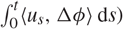 $\int_{0}^{t}\langle u_{s},\Delta\phi\rangle {\rm d}s)$, by property (6) (this fact together with the previous facts is used to treat the term
 $\int_{0}^{t}\langle u_{s},b(u_{s},m_{s})\cdot\nabla\phi\rangle {\rm d}s$, and the facts that Fζ is continuous and F̃ζ is bounded (these facts are used to deal with the m term). Moreover, b(u, m) converges locally uniformly in space when (u, m) converges in
 $C( L_{\rm loc}^{2}) \times C( L_{\rm loc}^{2})$. This last point is a delicate one, so in the next lines we prove it. Let us consider a sequence (uN, mN) converging in
 $L^2_{\rm loc}$; for fixed ε > 0 and x ∈ B(0, K), with K > 0
 \begin{align*} &|b(u^N,m^N)(x)-b(u,m)(x)| \\ &\qquad \leq \int_{\mathbb{R}^d} |g(|y-x|,u^N(\kern1pt y),m^N(\kern1pt y))-g(|y-x|,u(\kern1pt y),m(\kern1pt y))|{\rm d} y \\ &\qquad=\int_{B(0,R)} |g(|y-x|,u^N(\kern1pt y),m^N(\kern1pt y))-g(|y-x|,u(\kern1pt y),m^N(\kern1pt y))|{\rm d} y \\ &\qquad +\int_{B(0,R)^c} |g(|y-x|,u^N(\kern1pt y),m^N(\kern1pt y))-g(|y-x|,u(\kern1pt y),m(\kern1pt y))|{\rm d} y \\ &\qquad= I_1+I_2(R,N), \end{align*}
where, thanks to hypothesis (4), R can be chosen such that I 2(R, N) ≤ ε/2 uniformly in x. Regarding I 1, there exists N 0 such that
 \begin{equation*} I_1\leq \| Dg\| \int_{B(0,R)}|u^N(\kern1pt y)-u(\kern1pt y)|{\rm d} y\leq \frac{\varepsilon}{2} \quad\text{for all $N>N_0$. }\end{equation*}
Computations including the time component are straightforward. So, b(uN, mN) converges locally uniformly in space to b(u, m).
Thanks to continuity of the functional Ψφ, by the Portmanteau theorem,
 \begin{equation}Q( (u,m)\colon \Psi_{\phi}(u,m)>\delta) \leq\liminf_{k}Q^{N_{k}}( (u,m)\colon \Psi_{\phi}(u,m)> \delta).\end{equation}
Then, by Lemma 8,
 \begin{equation}Q( (u,m)\colon \Psi_{\phi}(u,m)>\delta) =0\end{equation}
for every δ > 0. By a classical argument, see [Reference Kipnis and Landim7],
 \begin{equation}Q( (u,m)\colon \Psi_{\phi}(u,m)=0 \text{ for all }\phi \in\mathcal{D}) =1.\end{equation}
Thus, Q is supported on weak solutions. In addition, by Corollary 1, u is also of class Lp(0, T;L 2(ℝd)) for some p > 2. With a proper choice of φ related to the heat kernel e−|x−y|2/(4t)/(4πt)d/2, we prove that u satisfies the mild formulation; it is straightforward to see that m satisfies the differential equation. Hence, we have proved that Q is supported by the set of mild solutions.
Proposition 5. Assume that u 1, m 1, u 2, and m 2 are functions of class C(L 2) such that (u 1, m 1) and (u 2, m 2) are mild solutions of system (2) corresponding to the same initial condition (u 0, m 0), with ut, mt ≥ 0 for every t ∈ [0, T]. Then (u 1, m 1) = (u 2, m 2).
Proof. Each ui, i = 1, 2, satisfies the identity
 \begin{equation}u_{t}^{i}(x)={\rm e}^{tA}u_{0}+\int_{0}^{t}\nabla\cdot {\rm e}^{(t-s)A} \bigg(u_{s}^{i}b\bigg(u_{s}^{i},F_{\zeta}\bigg( m_{0}(x),\int_{0}^{s}u_{r} ^{i}(x){\rm d} r\bigg) \bigg)\bigg){\rm d} s,\end{equation}
where we have used the explicit formula for (1b). This is a closed equation and we are going to prove from it that u 1 = u 2. A fortiori we also obtain m 1 = m 2, again from the explicit formula for (1b).
Assume by contradiction that u 1 ≠ u 2. Let t 0 ∈ [0, T) be the infimum of all t ∈ [0, T] such that  $u_{t}^{1}\neq u_{t}^{2}$. On [0, t 0] we have (u 1, m 1) = (u 2, m 2). On [t 0, T] we use the mild formula and property (3) to obtain
 \begin{align*} &\| u_{t}^{1}-u_{t}^{2}\| _{L^{2}} \\ &\qquad \leq\int_{t_{0}} ^{t}\| \nabla\cdot {\rm e}^{(t-s)A}(u_{s}^{1}b(u_{s}^{1},m_{s} ^{1})-u_{s}^{2}b(u_{s}^{2}, m_{s}^{2}))\| _{L^{2}}{\rm d} s \\ &\qquad \leq\int_{t_{0}}^{t}\frac{C}{|t-s|^{1/2}}\| u_{s}^{1}b(u_{s} ^{1},m_{s}^{1})-u_{s}^{2}b(u_{s}^{2},m_{s}^{2})\| _{L^{2}}{\rm d} s \\ &\qquad \leq\int_{t_{0}}^{t}\frac{C}{|t-s|^{1/2}}( \| b(u_{s}^{1},m_{s} ^{1})\| _{\infty}\| u_{s}^{1}-u_{s}^{2}\| _{L^{2}}+\| u_{s} ^{2}\| _{L^{2}}\| b(u_{s}^{1},m_{s}^{1})-b(u_{s}^{2},m_{s} ^{2})\| _{L^{\infty}}) {\rm d} s.\end{align*}
Recall that b is bounded, see (5), and that  $\| u_{s} ^{2}\| _{L^{2}}$ is bounded by assumption. Hence,
 \begin{equation}\left\| u_{t}^{1}-u_{t}^{2}\right\| _{L^{2}}\leq\int_{t_{0}}^{t}\frac {C}{|t-s|^{1/2}}( \| u_{s}^{1}-u_{s}^{2}\| _{L^{2} }+\| b(u_{s}^{1},m_{s}^{1})-b(u_{s}^{2},m_{s}^{2})\| _{L^{\infty}}) {\rm d} s.\end{equation}
From property (6) and Hölder’s inequality we have
 \begin{align*} |b(u_{s}^{1},m_{s}^{1})(x)-b(u_{s}^{2},m_{s}^{2})(x)| & \leq C\int _{\mathbb{R}^{d}}{\rm e}^{-|x-y|}( \vert u_{s}^{1}( y) -u_{s}^{2}( y) \vert +\vert m_{s}^{1}( y) -m_{s}^{2}( y) \vert ) {\rm d} y \\ & \leq C\| u_{s}^{1}-u_{s}^{2}\| _{L^{2}}+C\| m_{s}^{1}-m_{s}^{2}\| _{L^{2}}; \end{align*}
hence,
 \begin{align*} \left\| u_{t}^{1}-u_{t}^{2}\right\| _{L^{2}}\leq\int_{t_{0}}^{t}\frac {C}{|t-s|^{1/2}}( \| u_{s}^{1}-u_{s}^{2}\| _{L^{2} }+\| m_{s}^{1}-m_{s}^{2}\| _{L^{2}}) {\rm d} s. \end{align*}
Recalling the explicit formula for (1b), we have
 \begin{align*} \vert m_{s}^{1}\left( x\right) -m_{s}^{2}(x)\vert & =\left\vert F_{\zeta}\left( m_{0}(x),\int_{0}^{s}u_{r}^{1}(x){\rm d} r\right) -F_{\zeta}\left( m_{0}(x),\int_{0}^{s}u_{r}^{2}(x){\rm d} r\right) \right\vert \\ & \leq\| \partial_{b}F_{\zeta}\| _{\infty}\bigg\vert \int_{0}^{s}u_{r}^{1}(x){\rm d} r-\int_{0}^{s}u_{r}^{2}(x){\rm d} r\bigg\vert \\ & \leq C\int_{0}^{s}\vert u_{r}^{1}(x)-u_{r}^{2}(x)\vert {\rm d} r \\ &=C\int_{t_{0}}^{s}\vert u_{r}^{1}(x)-u_{r}^{2}(x)\vert {\rm d} r, \end{align*}
whence
 \begin{equation}\| m_{s}^{1}-m_{s}^{2}\| _{L^{2}}\leq C_{T}\int_{t_{0}} ^{s}\| u_{r}^{1}-u_{r}^{2}\| _{L^{2}}{\rm d} r.\end{equation}
Summarising, the function  $v_{t}\colon = \| u_{t}^{1}-u_{t}^{2}\|_{L^{2}}$ satisfies
 \begin{equation}v_{t}\leq\int_{t_{0}}^{t}\frac{C}{|t-s|^{1/2}}\bigg( v_{s}+ C_{T}\int_{t_{0} }^{s}v_{r}{\rm d} r\bigg) {\rm d} s.\end{equation}
Given t 1 ∈ [t 0, T], we set A (t 1) := supt∈[t 0,t 1] vt. Then, on the interval t ∈ [t 0, t 1], we have
 \begin{equation}v_{t}\leq\int_{t_{0}}^{t}\frac{C}{|t-s|^{1/2}}( A( t_{1}) +C_{T}^{\prime}A( t_{1}) ) {\rm d} s=C^{\prime\prime}A\left( t_{1}\right) \left( t-t_{0}\right) ^{1/2}.\end{equation}
It follows that
 \begin{equation}A\left( t_{1}\right) \leq C^{\prime\prime}A\left( t_{1}\right) \left( t_{1}-t_{0}\right) ^{1/2}.\end{equation}
If t 1 − t 0 > 0 is small enough, we deduce that A (t 1) = 0; hence, u 1 = u 2 on [t 0, t 1], in contradiction with the definition of t 0.
5. Simulations
The aim of this section is to show the flexibility of the model, namely how it may reveal different types of aggregations. For instance, we avoid an arbitrary concentration (even with infinitesimal noise), opposite to most of the models in the literature, but cover the case of concentration for the cases of single and multiple concentration points. Each numerical simulation shown below is given for the following choice of parameters: number of particles N = 100, parameter of diffusion σ 2 = 0.1, discretization of time dt = 10−4, kernel smoothing parameter β = 0.9, and, for the initial condition, we made a simple choice, choosing just a realization of the uniform distribution on the square [0, 2] × [0, 2].
5.1. Degenerate aggregation
Let us start from the most basic example, the case when each particle is attracted by the others. Recall that we model the interaction between individuals and the density of the population; hence, each individual is pushed to high population density regions. A standard choice for g could be
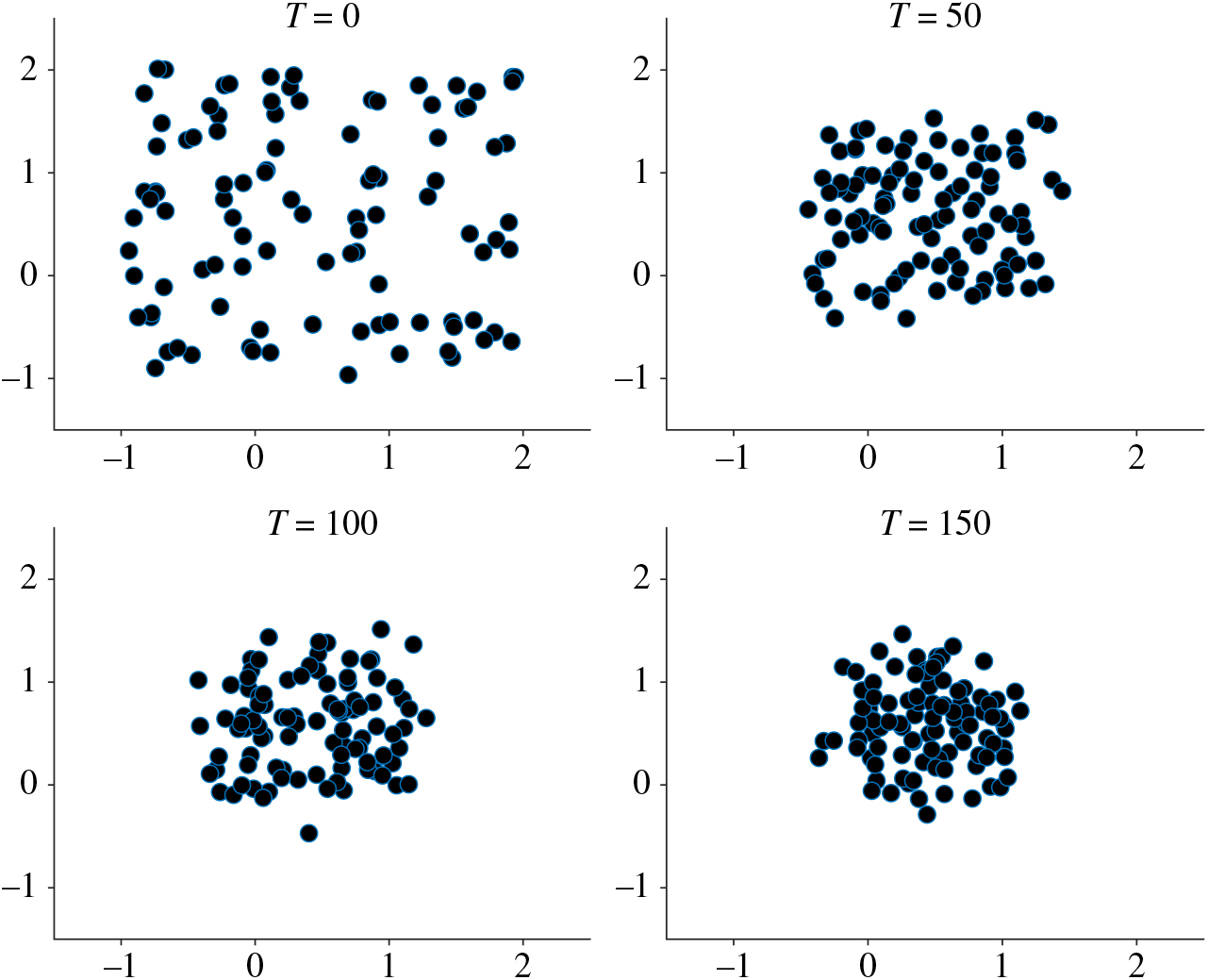
 \begin{equation}g(r,u)={\rm e}^{-r}\frac{u}{1+u} \quad\text{or}\quad g(r,u)={\rm e}^{-r}\tanh(u).\end{equation}
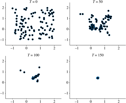
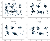
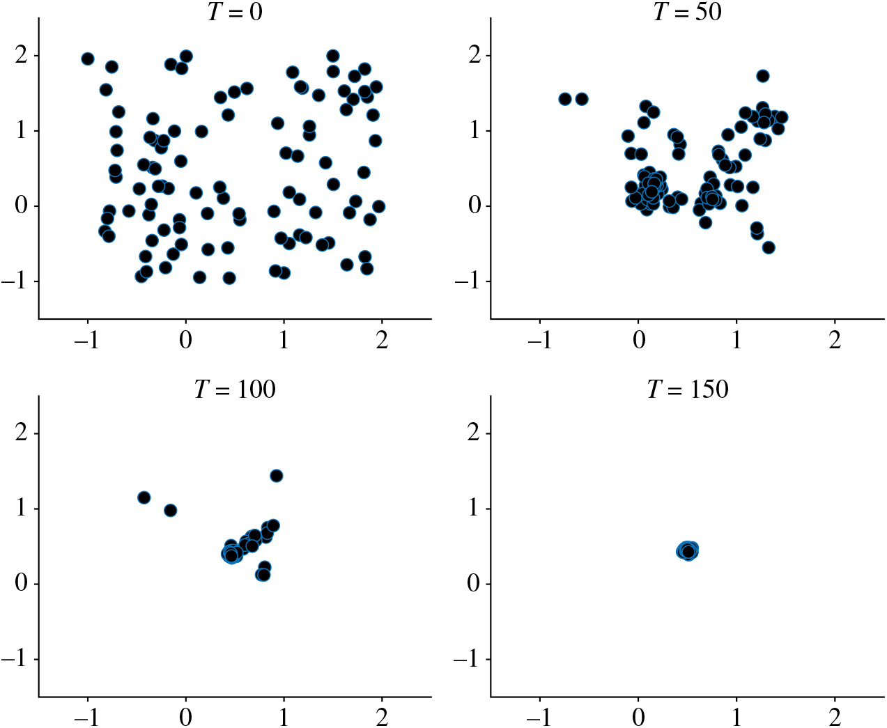
Note that, with this choice, cells continue to aggregate even at high density. The population mass tends to concentrate into a single point (see Figure 1).
Configuration of 100 particles at times T = 0, 50, 100, and 150 with g(r, u) = e−ru/(1 + u).
5.2. Moderate aggregation
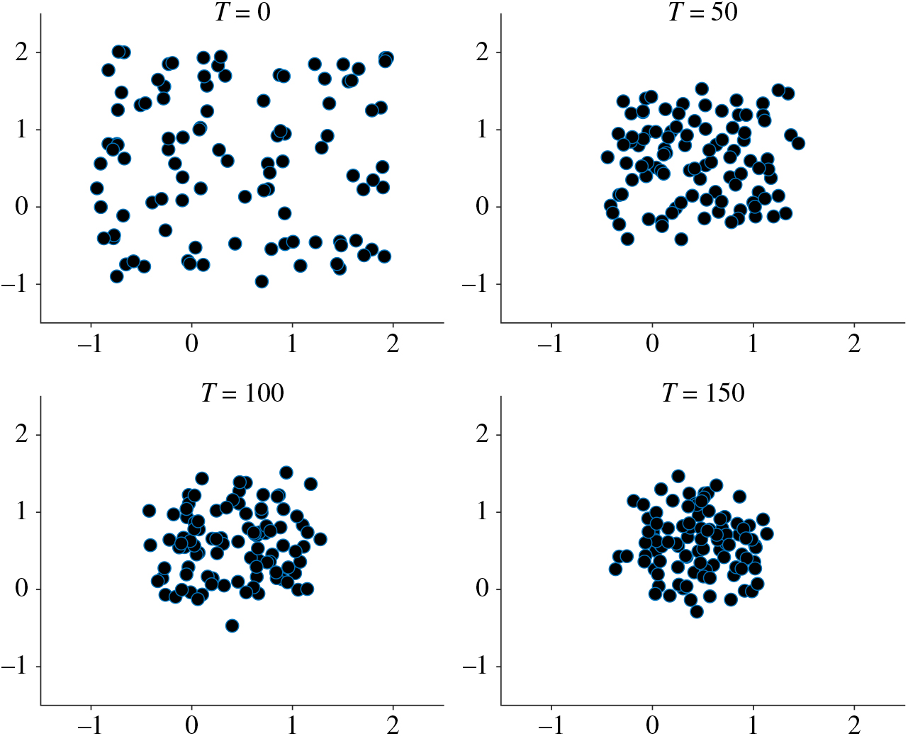
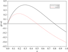
Let us now include a repulsive component in the force, to avoid collapse of the total mass (see Figure 2). The function g(r, u) we look for should have the following features (see Figure 3).
Configuration of 100 particles at times T = 0, 50, 100, and 150 with g(r, u) :=u log (r/u)/(1 - u log (r/u)).
Plot of the the function r ↦ g(r, u) for r = 0.8 (solid line) and r = 0.5 (dotted line).
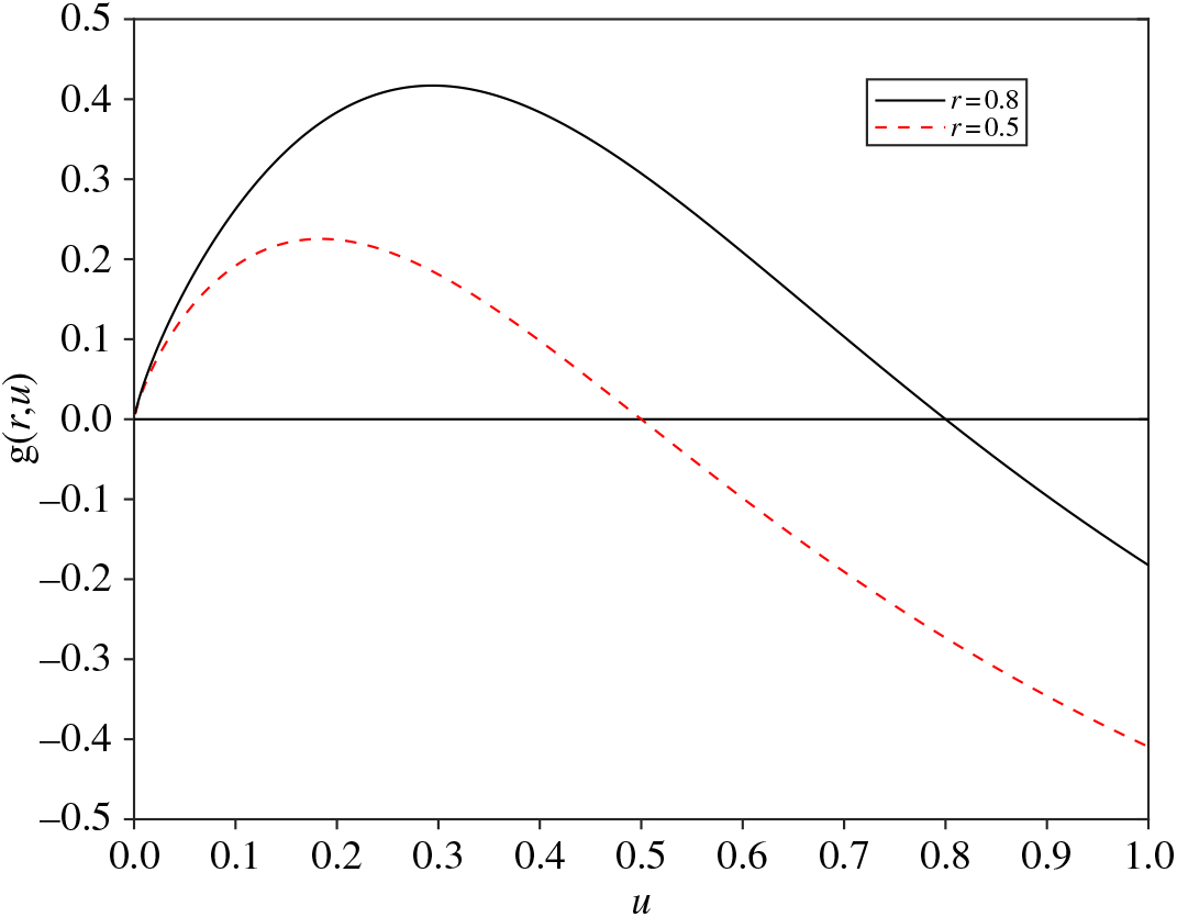
• Given the distance r, g(r, u) is such that the force is aggregative for small density and repulsive for large density. This behavior is natural for certain animals: each individual is attracted by its similar, but this changes when there are many individuals.
• There is an issue when we quantify small and large densities: this quantification should depend on distance. At large distances, we expect aggregation to be more relevant, with the individual tending to avoid only very large densities. On the other hand, at short distances, each individual is attracted only by very small densities.
The function we propose is
 \begin{equation}g(r,u)\colon = \frac{u\log\left( {r}/{u}\right) }{1-u\log\left({r}/{u}\right)}.\end{equation}
Another example could be
 \begin{equation}g(r,u)\colon = {\rm e}^{-r}\frac{u(\alpha-u)}{1+u},\end{equation}
where the parameter α can be interpreted as an index of overcrowding; choosing α properly, particles aggregate, without collapsing. The main drawback we have observed in simulations for this alternative is its strong sensitivity to the choice of parameter α with respect to the initial configuration. The first option we propose is more stable.
Note that the functions g(r, u) of this subsection are not products of functions of two single variables, namely, g(r, u) = g 1 (r) g 2 (u).
5.3. Aggregation in clusters
Returning to the first model, g(r, u) = e−ru/(1 + u), an interesting variant is when attraction happened only up to a certain distance (see Figure 4):
Configuration of 100 particles at times T = 0, 50, 100, and 150 with gR(r, u):= (u/(1 + u)) exp (− r 2/R) and R = 0.3.
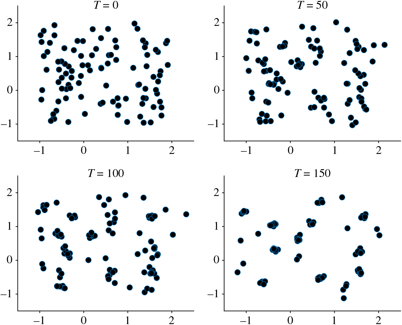
 \begin{equation}g_R(r,u)\colon = \frac{u}{1+u}\exp\left(\!-\frac{r^2}{R}\right)\!.\end{equation}
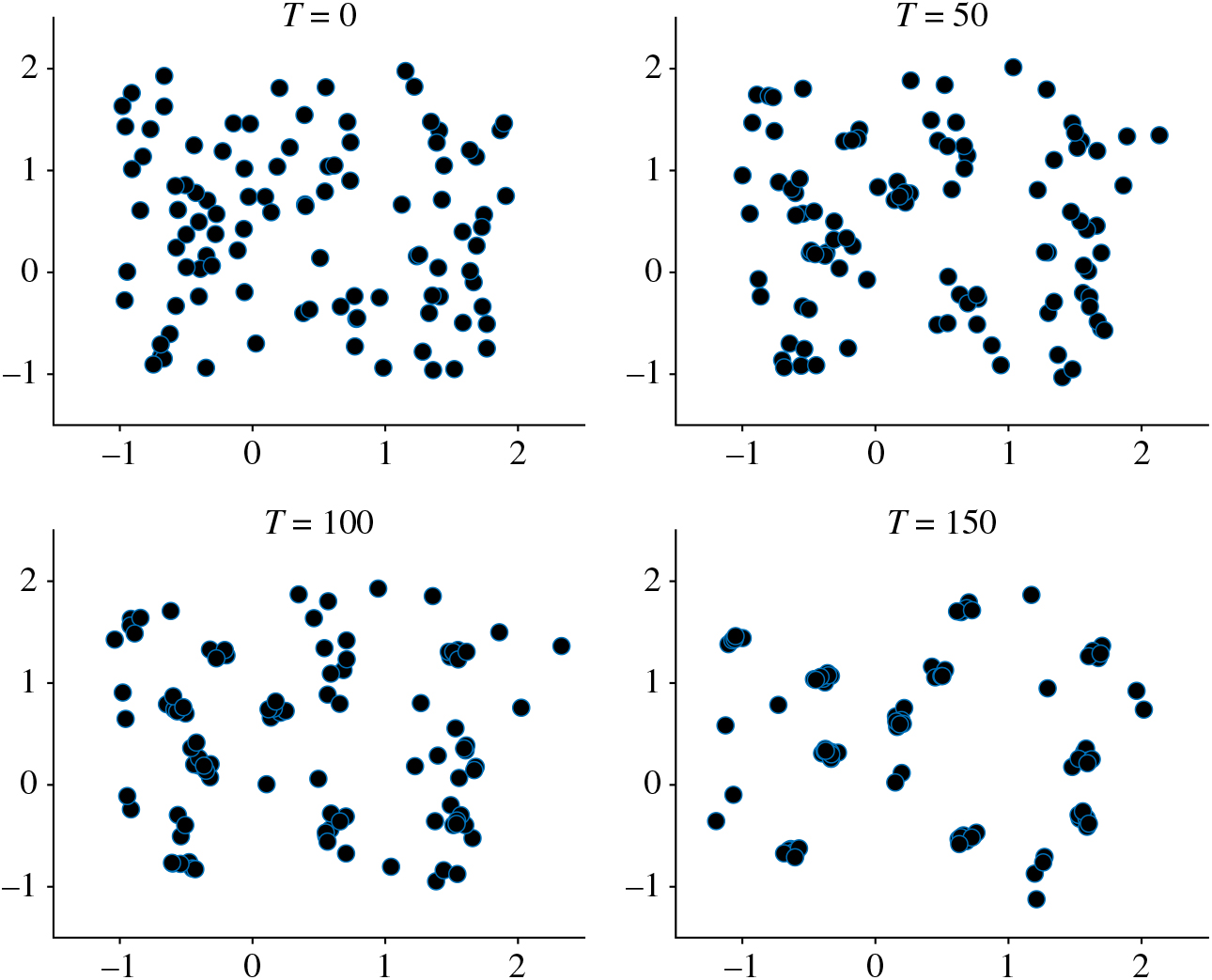
With this choice we observe the formation of clusters of individuals. Clearly, the parameter R influences the number of clusters that are generated: for large R, the population aggregates into a reduced number of clusters.
When t goes to infinity, if the noise is infinitesimal, each cluster reduces to a point, and maybe due to the noise, different clusters may meet and collapse.
5.4. Moderate aggregation in clusters
We may mix-up the previous two features. The following example has a tendency to construct clusters (see Figure 5), but they remain of finite size (independently of the noise):
Configuration of 100 particles at times T = 0, 50, 100, and 150 with gR(r, u): = (u(α − u)/(1 + u)) exp (− r 2/R), R = 0.3, and α = 1.3.
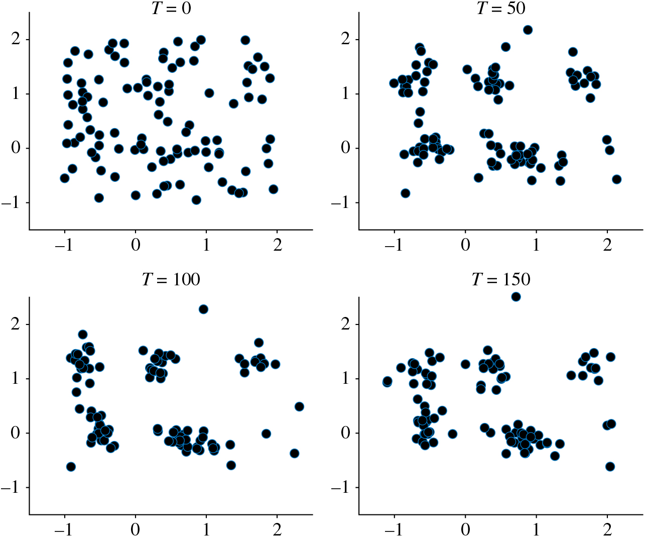
 \begin{equation}g_R(r,u)\colon = \frac{u(\alpha-u)}{1+u}\exp\left(\!-\frac{r^2}{R}\right).\end{equation}