2. Lifetime under varying stress levels

In this section we suggest a general stochastic model for the lifetime of a component operated under varying stress levels, and in Section 3 we will use it to model cascading failures. To model the component lifetime under varying stress levels, we will use the ALT model, which is based on the usual stochastic order, and the concept of virtual age. First we briefly introduce the ALT model; see also [Reference Cha5] and [Reference Cha, Mi and Yun6] for other reliability applications of the ALT model such as burn-in and standby systems. In introducing the ALT model we essentially follow the description of Cha, Mi, and Yun [Reference Cha, Mi and Yun6], with appropriate modifications. We first introduce the concept of the usual stochastic order, as follows.

Today’s highly reliable products may take too long to fail, and it may take an impractically long time to conduct a life testing. Thus, in this case, test units are subjected to a higher than usual level of load or stress to observe the failure times of the tested units in an affordable amount of testing time. This is the main objective of the ALT. After conducting the ALT, using the observed lifetimes obtained from the ALT, the actual lifetime distribution under the usual level of stress is predicted. See [Reference Nelson17] for background, basic theory, and examples for the ALT.

Let an absolutely continuous non-negative random variable Z be the lifetime of a component operated under the usual level of stress, and let G(t), ${\bar G}(t)$ , g(t), and r(t) be its cumulative distribution, survival, probability density, and failure rate functions, respectively. Also, let $Z_{\mathcal{AS}}$ denote the lifetime of a component operated under the accelerated stress level, with the corresponding distribution function $G_{\mathcal{AS}}(t)$ . Since the units are operated under accelerated stress during ALT, $Z_{\mathcal{AS}}$ would be stochastically smaller than Z, and it is thus natural to assume that

(1) \begin{equation} Z_{\mathcal{AS}} \leq_{st} Z.\end{equation}

By Definition 1, inequality (1) implies $G(t) \leq G_{\mathcal{AS}}(t)$ for all $ t\geq 0$ . Note that the distribution function of an absolutely continuous random variable is a continuous increasing function. Thus the relation $G(t) \leq G_{\mathcal{AS}}(t)$ for all $t\geq 0$ , or inequality (1), is equivalent to the following relation:

(2) \begin{equation} G_{\mathcal{AS}}(t)=G(\rho(t))\quad\text{for all } t \geq 0,\end{equation}

where $\rho({\cdot})$ is non-decreasing, $\rho(t) \geq t$ for all $t \geq 0$ , and $\rho(0)=0$ . To describe the lifetime distribution of units operated under an accelerated environment, Meeker and Escobar [Reference Meeker and Escobar13] also suggested the general model given in (2). We thus follow the general model in (2) as the lifetime distribution of units operated under accelerated stress level. From (2), by using the ‘failure rate function under the usual stress level’ r(t), the corresponding survival function ${\bar G}_{\mathcal{AS}}(t)$ can be written as

(3) \begin{equation}{\bar G}_{\mathcal{AS}}(t)=\exp\biggl\{-\int_{0}^{\rho(t)}r(x)\,{\mathrm{d}} x\biggr\},\end{equation}

where $\rho(t)$ can be interpreted as the ‘degradation function’ and $\rho'(t)$ as the ‘rate of degradation’ (see Finkelstein [Reference Finkelstein7, Reference Finkelstein8, Reference Finkelstein9]). In practice, a simple linear function $\rho(t)=\rho t$ , $t\geq0$ , is frequently applied (see [Reference Leemis12]).

Suppose a component that has been operated during (0, u] without failure under the accelerated stress level now starts to operate under the usual level of stress. Then, in this case, the future reliability performance of this component under the usual level of stress will not be equal to that of a component which has been operated during (0,u] without failure under the usual stress level, because these two components have been operated under different stress levels. Since the ageing process under the higher level of stress is accelerated, the ‘virtual age’ of this component would be greater than u. Thus it is assumed that the survival function for the residual lifetime of this component under the usual stress level is given by

(4) \begin{equation} \dfrac {{\bar G}(a(u)+t)}{{\bar G}(a(u))} = \exp\biggl\{-\int_{0}^{t} r(a(u)+x) \,{\mathrm{d}} x\biggr\} , \quad t\geq 0,\end{equation}

where a(u) satisfies $a(u) \geq u$ , for all $u \geq 0$ , $a(0)=0$ , and is assumed to be a non-decreasing function.

As in the cumulative exposure model in [Reference Nelson17], if the virtual age a(u) is assumed to yield the same cumulative failure probability of units as the age u does in the accelerated level of stress, that is, if we assume

\begin{equation*} G(a(u))= G_{\mathcal{AS}}(u)\quad\text{for all } u \geq 0,\end{equation*}

then it obviously holds that

(5) \begin{equation}a(u)=\rho(u)\quad\text{for all } u \geq 0.\end{equation}

The relation in (5) is typically assumed in ALT (see [Reference Nelson17]), and throughout this paper we assume this relation.

Based on the ALT model and the concept of virtual age described above, we now discuss the lifetime of a component operated under varying stress levels. Suppose a system having its baseline failure rate (the failure rate in the usual stress level) r(t) starts to operate at time 0 under a stress level which is higher than the usual level and, as it operates, the stress level changes to another one which is higher than the usual level at times $0<t_1<t_2<\cdots.$ For each interval $[t_{i-1},\,t_{i})$ , $i=1,2,\ldots,$ with $t_0\equiv0$ , the degradation function corresponding to the stress level in this interval is given by $\rho_i(t)$ , $i=1,2,\ldots,$ respectively. Let T denote the lifetime of the system operated under the described environment with the changes of stress level. Then its survival and conditional survival functions are obtained in the following proposition.

Proposition 1. For $n\geq 0$ and $t\in [t_n, t_{n+1})$ ,

(6) \begin{equation}\mathbb{P} (T>t)=\exp\biggl\{ -\int_{0}^{\sum_{i=1}^{n} \rho_i(t_i-t_{i-1})+\rho_{n+1}(t-t_n)} r(x)\,{\mathrm{d}} x\biggr\},\end{equation}

where $\sum_{i=1}^{n} ({\cdot}) \equiv 0$ if $n=0$ . Furthermore, for $n\geq 1$ , $j\leq n$ , and $t\in [t_n, t_{n+1})$ ,

(7) \begin{equation}\mathbb{P} (T>t\mid T>t_j)=\exp\biggl\{ -\int_{\sum_{i=1}^{j}\rho_i(t_i-t_{i-1}) }^{\sum_{i=1}^{n} \rho_i(t_i-t_{i-1})+\rho_{n+1}(t-t_n)} r(x)\,{\mathrm{d}} x\biggr\}.\end{equation}

Proof. For $n=0$ , from (2) and (3), it is clear that

\begin{equation*}\mathbb{P} (T>t)=\exp\biggl\{-\int_{0}^{\rho_{1}(t)} r(x)\,{\mathrm{d}} x\biggr\}.\end{equation*}

Observe that, for $n\geq 1$ ,

(8) \begin{equation}\mathbb{P} (T>t)=\biggl(\prod_{j=1}^{n} \mathbb{P} (T>t_{j}\mid T>t_{j-1}) \biggr)\cdot \mathbb{P} (T>t\mid T>t_{n}).\end{equation}

In (8),

\begin{equation*}\mathbb{P} (T>t_1)=\exp\biggl\{-\int_{0}^{\rho_{1}(t_1)} r(x)\,{\mathrm{d}} x\biggr\}.\end{equation*}

Note that at time $t_1$ , due to (4)–(5), the virtual age of the system is given by $\rho_1(t_1)$ and, in the interval $[t_1, t_2)$ , the component is operated under the accelerated stress level specified by $\rho_2(t)$ . Thus

\begin{align*}\mathbb{P} (T>t_{2}\mid T>t_{1})&= \exp\biggl\{-\int_{0}^{\rho_{2}(t_2-t_1)} r(\rho_{1}(t_1)+x)\,{\mathrm{d}} x\biggr\}\\* &= \exp\biggl\{-\int_{\rho_{1}(t_1)}^{\rho_{1}(t_1)+\rho_{2}(t_2-t_1)} r(x)\,{\mathrm{d}} x\biggr\},\end{align*}

and similarly

\begin{equation*}\mathbb{P} (T>t_{j}\mid T>t_{j-1})= \exp\biggl\{ -\int_{\sum_{i=1}^{j-1}\rho_i(t_i-t_{i-1}) }^{\sum_{i=1}^{j} \rho_i(t_i-t_{i-1})} r(x)\,{\mathrm{d}} x\biggr\}, \quad j=3,\ldots,n,\end{equation*}

and

\begin{equation*}\mathbb{P} (T>t\mid T>t_{n})= \exp\biggl\{ -\int_{\sum_{i=1}^{n}\rho_i(t_i-t_{i-1}) }^{\sum_{i=1}^{n} \rho_i(t_i-t_{i-1})+\rho_{n+1}(t-t_n)} r(x)\,{\mathrm{d}} x\biggr\}.\end{equation*}

Then, by applying (8), we have $\mathbb{P} (T>t)$ in (6). The residual lifetime distribution $\mathbb{P} (T> t\mid T>t_j)$ in (7) can be directly obtained by using $\mathbb{P} (T>t)$ in (6). □

It can be seen from Proposition 1 that, given the stress level changes until time t, the survival probability of the component can be obtained by calculating the integral of r(x) from 0 to $ \sum_{i=1}^{n} \rho_i(t_i-t_{i-1})+\rho_{n+1}(t-t_n)$ and then by taking the exponential formula. In this case, the function

\begin{equation*}\sum_{i=1}^{n} \rho_i(t_i-t_{i-1})+\rho_{n+1}(t-t_n)\end{equation*}

can be interpreted as the ‘cumulative degradation’ until time t.

3. New stochastic model for cascading failures

In this section, based on the discussion given in Section 2, we suggest a new stochastic model for cascading failures. In [Reference Lee and Cha11], basically, the lifetime of a k-out-of-n system subject to cascading failures was modelled assuming that the failure rates of the remaining components increase as the number of failed components in the system increases. Then, interpreting the sequential failures of the components in the system as the events in a point process, they specified the corresponding stochastic intensity function to obtain the survival function of the system (see [Reference Lee and Cha11] for more details). For the reason described in [Reference Lee and Cha11], we will also consider the many-valued cascading model in this paper. In the studies of [Reference Swift19] and [Reference Lee and Cha11], it is assumed that, after a failure of a component in the system, the load or stress on the remaining components is increased and the failure rate of each remaining component increases but, after time $\delta$ , this effect of increased stress vanishes and the failure rate drops back to the previous level. For convenience, we call this interval of length $\delta$ during which the remaining components are affected the ‘effective period’. In the many-valued cascading model, the total increment size in the failure rate of a remaining component is proportional to the total number of overlapping effective periods, whereas in the two-valued cascading model, the total increment size in the failure rate of a remaining component is always fixed regardless of the total number of overlapping effective periods.

In this paper we also consider a k-out-of-n system subject to cascading failures. The n components in the system have the same general failure rate $\lambda(t)$ (which corresponds to the failure rate of a component under the usual level of stress). As in [Reference Lee and Cha11], we assume that, after a failure of a component in the system, the load or stress on the remaining components is increased, but the effect of increased stress on the remaining components is described by the ALT model introduced in Section 2. Under this model, to apply the point process approach suggested in [Reference Lee and Cha11], it is necessary to obtain the stochastic intensity function, regarding the sequential failures of the components in the system as the events in a point process. As in [Reference Lee and Cha11], we let $0\leq S_1\leq S_2 \leq \cdots \leq S_{n-k} $ denote the sequential failure points of the components in the k-out-of-n system and let N(t) be the total number of component failures observed in (0, t]. Then the system survival function for the k-out-of-n system is defined by $\mathbb{P} (N(t)\leq n-k)$ , which will be derived by using the stochastic intensity function of $\{N(t)$ , $t\geq0\}$ .

The stochastic intensity function given the history up to time t, ${\mathcal{H}}_{t-}=(N(t-)=l$ , $S_1=s_1$ , $S_2=s_2,\ldots,S_{l}=s_l)$ , is defined by (see e.g. [Reference Aven and Jensen1] and [Reference Aven and Jensen2])

\begin{equation*} \lambda_{t} \equiv \lim_{\Delta t\rightarrow 0} \dfrac{\mathbb{P} (N(t,t+\Delta t)=1\mid {\mathcal{H}}_{t-})}{\Delta t} = \lim_{\Delta t\rightarrow 0} \dfrac{E[N(t, t+\Delta t)\mid {\mathcal{H}}_{t-}]}{\Delta t},\end{equation*}

where $N(t_1,t_2)$ , $t_1<t_2$ , represents the number of events in $[t_1 , t_2)$ . For convenience, the stochastic intensity $\lambda_{t}$ , when ${\mathcal{H}}_{t-}=(N(t-)=l$ , $S_1=s_1$ , $S_2=s_2,\ldots,S_{l}=s_l)$ , will be denoted by $\lambda_{l}(t\mid s_1,s_2,\ldots,s_l)$ , $l=0, 1,2,\ldots, n-k$ , and, when $l=0$ , the notation $\lambda_{l}(t\mid s_1,s_2,\ldots,s_l)$ will be written as $\lambda_{0}(t)$ . Obviously $\lambda_{0}(t)=n\lambda(t)$ .

In the k-out-of-n system considered, the stress level (i.e. the total number of overlapping effective periods) of a remaining component changes dynamically depending on the failure times of components which have failed previously, and it is a crucial element in describing the stochastic model because we have to apply different degradation functions depending on the stress level. 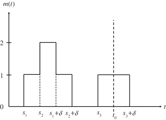To obtain $\lambda_{l}(t\mid s_1,s_2,\ldots,s_l)$ , $l=1,2,\ldots, n-k$ , we now define some necessary notations to represent this dynamic stress level changes in the system, referring to Figure 1.

Figure 1:

Realization of m(t) for the component which fails last in a 1-out-of-4 system when $s_1,s_2,s_3$ are given.

Define m(t), $t\geq 0$ , as the total number of overlapping effective periods at time t, and define it as a ‘right-continuous’ function, which can be mathematically defined as

\begin{equation*}m(t)=\sum_{i=1}^{N(t)}\alpha_\delta(t-s_i),\end{equation*}

where

(9) \begin{equation}\alpha_\delta(t)=\begin{cases}1 &\text{if $0 \leq t<\delta$,} \\[4pt] 0 &\text{otherwise.}\end{cases}\end{equation}

By convention, $m(t)=0$ if $N(t)=0$ . Thus m(t) represents the level of stress imposed on each remaining component at time t and the minimum and maximum values of it are 0 and $n-k$ , respectively, for the k-out-of-n system considered. Regarding m(t) as a stochastic process $\{m(t),\, t\geq0\}$ , we can define the stress level change times $0\equiv v_0<v_1<v_2<\cdots$ . Furthermore, define h(t) as the total number of level changes (i.e. jump up or jump down) in (0, t). Then, given ${\mathcal{H}}_{t-}=(N(t-)=l$ , $S_1=s_1$ , $S_2=s_2,\ldots,S_{l}=s_l)$ , h(t) depends on the positions of $s_1,s_2,\ldots,s_l$ and the size of $\delta$ (see Figure 1), which has minimum and maximum values l and 2l, respectively. Then the sequential points of stress level changes in (0, t) are denoted by $v_1,v_2,\ldots,v_{h(t)}$ . To aid understanding of these notations, a realization of m(t) is given in Figure 1, assuming that the system is a 1-out-of-4 system.

In the example in Figure 1, $h(t_0)=5$ , $v_1=s_1$ , $v_2=s_2$ , $v_3=s_1+\delta$ , $v_4=s_2+\delta$ , and $v_5=s_3$ . Note that Figure 1 may also correspond to the realization of m(t) of the non-failed components in other system configurations.

We assume that when there are i overlapping effective periods in total, the degradation function corresponding to this stress level is given by $\rho_i (t)$ , and its derivative $\rho^{\prime}_i (t)$ exists, for $i=0,1,2,\ldots,n-k$ . As before, $\rho_i({\cdot})$ is non-decreasing, $\rho_i(t) \geq t$ for all $t \geq 0$ , $\rho_i(0) =0$ , and it would be reasonable to assume that $\rho_i(t) \geq \rho_{i-1}(t)$ , for all $ t\geq0$ , for $i=1,2,\ldots,n-k$ , with $\rho_0(t) = t$ for all $t\geq0$ . Let $T_S$ denote the lifetime of the system. Then the stochastic intensity functions and the survival function of the system are given in the following theorem.

Theorem 1. Under the proposed model and assumptions, the stochastic intensity functions are given by

\begin{equation*} \lambda_{j}(t\mid s_1,s_2,\ldots,s_j)=\begin{cases}\lambda_0(t)=n\lambda(t) & j=0, \\[4pt](n-j)\rho^{\prime}_{m(v_{h(t)})}(t-v_{h(t)})\lambda(\varphi_j(t)) & j=1,2,\ldots,n-k,\end{cases}\end{equation*}

where, for given $0<s_1<s_2<\cdots<s_j \leq t$ ,

\begin{equation*}\varphi_j(t) \equiv \int_{0}^{t}\rho^{\prime}_{m(v_{h(x)})}(x-v_{h(x)})\,{\mathrm{d}} x=\sum_{i=1}^{h(t)} \rho_{m(v_{i-1})}(v_i-v_{i-1})+\rho_{m(v_{h(t)})}(t-v_{h(t)}).\end{equation*}

The survival function of the system is given by

\begin{align*}\mathbb{P} (T_S>t)&=\exp\biggl\{-\int_{0}^{t}\lambda_0(x)\,{\mathrm{d}} x\biggr\}\\[3pt] &\quad\, +\sum_{l=1}^{n-k} \int_{0}^{t} \int_{0}^{s_l}\cdots\int_{0}^{s_3}\int_{0}^{s_2} \prod_{j=0}^{l-1} \biggl[\lambda_{j}(s_{j+1}\mid s_1,s_2,\ldots,s_j) \\[3pt] & \quad\, \times \exp\biggl\{-\int_{\varphi_j(s_j)}^{ \varphi_j(s_{j+1})} (n-j) \lambda(x)\,{\mathrm{d}} x\biggr\}\biggr] \\[3pt] &\quad\, \times \exp\biggl\{-\int_{\varphi_l(s_l)}^{ \varphi_l(t)} (n-l) \lambda(x)\,{\mathrm{d}} x\biggr\} \,{\mathrm{d}} s_1 \,{\mathrm{d}} s_2 \cdots {\mathrm{d}} s_{l-1}\,{\mathrm{d}} s_{l},\end{align*}

where $\varphi_0(t)=t$ , for all $ t \geq 0$ , and $s_0\equiv0$ ,

\begin{equation*}\int_{0}^{t} \int_{0}^{s_l}\cdots\int_{0}^{s_3}\int_{0}^{s_2} ({\cdot}) \,{\mathrm{d}} s_1 \,{\mathrm{d}} s_2 \cdots {\mathrm{d}} s_{l-1}\,{\mathrm{d}} s_{l} =\int_{0}^{t} ({\cdot}) \,{\mathrm{d}} s_1\end{equation*}

when $l=1$ , $\sum_{l=1}^{n-k}({\cdot})\equiv 0$ when $n=k$ .

Proof. Let $T_C$ denote the lifetime of a ‘component in the system’. Then, given ${\mathcal{H}}_{t-}=(N(t-)=j$ , $S_1=s_1$ , $S_2=s_2,\ldots,S_{j}=s_j)$ and $T_C>s_j$ , the conditional survival function of $T_C$ is defined as

(10) \begin{align} &\mathbb{P} (T_C>t\mid T_C>s_j,\, S_1=s_1,\, S_2=s_2, \ldots, S_j=s_j)\notag \\[5pt] &\qquad =\dfrac{\mathbb{P} (T_C>t\mid S_1=s_1,\, S_2=s_2, \ldots, S_j=s_j)}{\mathbb{P} (T_C>s_j\mid S_1=s_1,\, S_2=s_2, \ldots, S_j=s_j)}.\end{align}

As discussed in Proposition 1 and the remark given after it, to calculate the survival probabilities in (10), the calculation of the ‘cumulative degradation’ is crucial. Note that given ${\mathcal{H}}_{t-}=(N(t-)=j$ , $S_1=s_1$ , $S_2=s_2,\ldots,S_{j}=s_j)$ , in [0, t), we have to consider in total $h(t)+1$ intervals: $[v_{i-1},v_{i})$ , $i=1,2,\ldots, h(t)$ , and $[v_{h(t)},t)$ . Note that the stress level in the interval $[v_{i-1},v_{i})$ is given by $m(v_{i-1})$ , $i=1,2,\ldots, h(t)$ , and that in the interval $[v_{h(t)},t)$ is given by $m(v_{h(t)})$ . Thus the cumulative degradation until time t is given by

\begin{equation*}\varphi_j(t) \equiv\sum_{i=1}^{h(t)} \rho_{m(v_{i-1})}(v_i-v_{i-1})+\rho_{m(v_{h(t)})}(t-v_{h(t)}),\end{equation*}

which can be equivalently expressed as the integration of the rate of degradation in the interval (0, t):

(11) \begin{equation}\varphi_j(t)=\int_{0}^{t}\rho^{\prime}_{m(v_{h(x)})}(x-v_{h(x)})\,{\mathrm{d}} x.\end{equation}

Then, from Proposition 1,

(12) \begin{equation}\mathbb{P} (T_C>t\mid T_C>s_j,\, S_1=s_1,\, S_2=s_2, \ldots, S_j=s_j)=\exp\biggl\{-\int_{\varphi_j(s_j)}^{\varphi_j(t)} \lambda(x)\,{\mathrm{d}} x\biggr\}.\end{equation}

From (12), the failure rate of a remaining component in the system when ${\mathcal{H}}_{t-}=(N(t)=j$ , $S_1=s_1$ , $S_2=s_2,\ldots,S_{j}=s_j)$ is given by

(13) \begin{equation}\dfrac{-({{{\mathrm{d}}}/{{{\mathrm{d}} t}}})\mathbb{P} (T_C>t\mid T_C>s_j,\, S_1=s_1,\, S_2=s_2, \ldots, S_j=s_j)}{\mathbb{P} (T_C>t\mid T_C>s_j,\, S_1=s_1,\, S_2=s_2, \ldots, S_j=s_j)}=\rho^{\prime}_{m(v_{h(t)})}(t-v_{h(t)})\lambda(\varphi_j(t)),\end{equation}

and, given ${\mathcal{H}}_{t-}=(N(t-)=j$ , $S_1=s_1$ , $S_2=s_2,\ldots,S_{j}=s_j)$ , as there are in total $(n-j)$ remaining components in the system, the stochastic intensity function is given by

\begin{equation*}\lambda_{j}(t\mid s_1,s_2,\ldots,s_j)= (n-j)\rho^{\prime}_{m(v_{h(t)})}(t-v_{h(t)})\lambda(\varphi_j(t)).\end{equation*}

Now we will derive the survival function of the system. Note that the joint distribution of $(N(t)=l$ , $S_1=s_1$ , $S_2=s_2,\ldots,S_l=s_l)$ is given by

\begin{align*}&\prod_{j=0}^{l-1} [\lambda_{j}(s_{j+1}\mid s_1,s_2,\ldots,s_j) \mathbb{P} (S_{j+1}>s_{j+1}\mid S_1=s_1,\, S_2=s_2, \ldots, S_j=s_j)]\\*&\quad\, \times \mathbb{P} (S_{l+1}>t\mid S_1=s_1,\, S_2=s_2, \ldots, S_l=s_l),\end{align*}

where

\begin{equation*}\mathbb{P} (S_{j+1}>s_{j+1}\mid S_1=s_1,\, S_2=s_2, \ldots, S_j=s_j)\equiv \mathbb{P} (S_1>s_1)=\exp\biggl\{-\int_{0}^{s_1}\lambda_0(x)\,{\mathrm{d}} x\biggr\}\end{equation*}

for $j=0$ and $0<s_1<s_2 < \cdots < s_l<t$ . Thus $\mathbb{P} (N(t)=l)$ can be obtained by

\begin{align*}\mathbb{P} (N(t)=l) &= \int_{0}^{t} \int_{0}^{s_l}\cdots\int_{0}^{s_3}\int_{0}^{s_2} \prod_{j=0}^{l-1} \bigl[\lambda_{j}(s_{j+1}\mid s_1,s_2,\ldots,s_j) \\*&\quad\, \times \mathbb{P} (S_{j+1}>s_{j+1}\mid S_1=s_1,\, S_2=s_2, \ldots, S_j=s_j)\bigr] \\*&\quad\, \times \mathbb{P} (S_{l+1}>t\mid S_1=s_1,\, S_2=s_2, \ldots, S_l=s_l) \,{\mathrm{d}} s_1 \,{\mathrm{d}} s_2 \cdots {\mathrm{d}} s_{l-1}\,{\mathrm{d}} s_{l},\end{align*}

where

\begin{equation*}\mathbb{P} (S_{j+1}>s_{j+1}\mid S_1=s_1,\, S_2=s_2, \ldots, S_j=s_j)=\exp\biggl\{-\int_{\varphi_j(s_j)}^{ \varphi_j(s_{j+1})} (n-j) \lambda(x)\,{\mathrm{d}} x\biggr\}\end{equation*}

and

\begin{equation*}\mathbb{P} (S_{l+1}>t\mid S_1=s_1,\, S_2=s_2, \ldots, S_l=s_l) =\exp\biggl\{-\int_{\varphi_l(s_l)}^{ \varphi_l(t)} (n-l) \lambda(x)\,{\mathrm{d}} x\biggr\}.\end{equation*}

Then the survival function of the system is given by

\begin{equation*}\hspace*{43pt}\mathbb{P} (T_S>t) =\sum_{l=0}^{n-k} \mathbb{P} (N(t)=l)= \exp\biggl\{-\int_{0}^{t} \lambda_0(u)\,{\mathrm{d}} u\biggr\} +\sum_{l=1}^{n-k} \mathbb{P} (N(t)=l).\hspace*{43pt}\square\end{equation*}

Remark 1. In differentiating $\varphi_j(t)$ in (13), if t is between two consecutive jump points (i.e. discontinuity points) of the function $m({\cdot})$ , h(x) in the interval $[t-\Delta t, t+\Delta t]$ for an infinitesimal value $\Delta t$ is fixed by h(t), and thus the derivative of $\varphi_j(t)$ in (11) is given by

\begin{equation*}\rho^{\prime}_{m(v_{h(t)})}(t-v_{h(t)}).\end{equation*}

Observe that the function $\varphi_j(t)$ may not be differentiable when t is a discontinuity point of the function $m({\cdot})$ because the left and right derivatives are not equal. In this case we can assign the left derivative to the derivative of $\varphi_j(t)$ , and this does not affect the survival function in Theorem 1 because the derivative of $\varphi_j(t)$ is just integrated in the survival function.

From Theorem 1, it can be shown that the failure rate of the system, denoted by $r_S(t)$ , is given by

\begin{align*} r_S(t) & =\dfrac{1}{\mathbb{P} (T_S>t)} \\* &\quad\, \times \biggl[\int_{0}^{t} \int_{0}^{s_{n-k}}\cdots\int_{0}^{s_3}\int_{0}^{s_2} \prod_{j=0}^{n-k-1} \biggl[\lambda_{j}(s_{j+1}\mid s_1,s_2,\ldots,s_j) \\*&\quad\, \times \exp\biggl\{-\int_{\varphi_j(s_j)}^{ \varphi_j(s_{j+1})} (n-j) \lambda(x)\,{\mathrm{d}} x\biggr\}\biggr] \\&\quad\, \times \lambda_{n-k}(t\mid s_1,s_2,\ldots,s_{n-k})\\*&\quad\, \times \exp\biggl\{-\int_{\varphi_{n-k}(s_{n-k})}^{ \varphi_{n-k}(t)} k \lambda(x)\,{\mathrm{d}} x\biggr\} \,{\mathrm{d}} s_1 \,{\mathrm{d}} s_2 \cdots {\mathrm{d}} s_{n-k-1}\,{\mathrm{d}} s_{n-k}\biggr],\end{align*}

where

\begin{equation*}\int_{0}^{t} \int_{0}^{s_{n-k}}\cdots\int_{0}^{s_3}\int_{0}^{s_2} ({\cdot}) \,{\mathrm{d}} s_1 \,{\mathrm{d}} s_2 \cdots {\mathrm{d}} s_{n-k-1}\,{\mathrm{d}} s_{n-k} =\int_{0}^{t} ({\cdot}) \,{\mathrm{d}} s_1\end{equation*}

when $n-k=1$ .

Now let us consider a meaningful specific case when $\rho^{\prime}_i(t)=1+i\rho $ , $i=1,2,\ldots, n-k$ . That is, in this case the degradation rate of the component is proportionally increasing in the number of overlapping effective periods. In this specific case, the formulas in Theorem 1 can be simplified as follows.

Corollary 1. If $\rho^{\prime}_i(t)=1+i\rho$ , $i=1,2,\ldots, n-k$ , then $\varphi_j(t)$ is given by

\begin{equation*}\varphi_j(t) = t+\rho \sum_{i=1}^{j} (\!\min(s_i+\delta, t)-s_i), \quad j=1,2,\ldots,n-k,\end{equation*}

and the stochastic intensity functions are given by

\begin{equation*}\lambda_{j}(t\mid s_1,s_2,\ldots,s_j)=\begin{cases}\lambda_0(t)=n\lambda(t) & j=0,\\[4pt] (n-j)(1+\rho \sum_{i=1}^{j} \alpha_\delta(t-s_i))\lambda(\varphi_j(t)) & j=1,2,\ldots,n-k,\end{cases}\end{equation*}

where function $\alpha_\delta ({\cdot})$ is defined in (9).

Proof. Observe that, given $0<s_1<s_2<\cdots<s_j \leq t$ , the degradation rate at time t is given by

\begin{equation*}1+\rho \sum_{i=1}^{j} \alpha_\delta(t-s_i)\end{equation*}

and the cumulative degradation in this case is obtained by

\begin{equation*}\hspace*{40pt}\varphi_j(t) =\int_{0}^{t}1+\rho \sum_{i=1}^{j} \alpha_\delta(x-s_i)\,{\mathrm{d}} x=t+\rho \sum_{i=1}^{j} (\!\min(s_i+\delta, t)-s_i),\hspace*{50pt}\square\end{equation*}

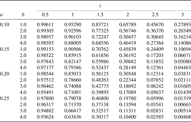
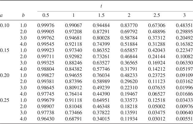
Example 1. In this example we investigate the effect of the system configuration, the component failure rate $\lambda(t)$ , and the degradation function $\rho_i(t)$ on the system lifetime. We consider 3-out-of-5 and 4-out-of-5 systems. In each system we assume that $\lambda(t)=at$ for all $ t \geq0$ , and $\rho_i(t)=(1+bi)t$ for all $ t \geq0$ , $1\leq i\leq n-k$ , where $a>0$ and $b>0$ , with $\delta=0.5$ . Thus, as the parameter b increases, the corresponding degradation rate at each stress level also increases. For different system configurations and different sets of values of a and b, the values of the system survival function $\mathbb{P} (T_S>t)$ are obtained in Tables 1 and 2. As can be seen by comparing the tables, the survival function of 3-out-of-5 systems is larger than that of 4-out-of-5 systems. This result is clear from the definition of the k-out-of-n system and also from the formula $\mathbb{P} (T_S>t)$ given in Theorem 1, which is increasing in $n-k$ . Furthermore, as the failure rate increases (i.e. as parameter a increases) and the degradation rate at each stress level increases (i.e. as parameter b increases), the survival function of the system decreases.

Table 1:

The values of the system survival function $\mathbb{P} (T_S>t)$ for 4-out-of-5 systems and various a and b.

Table 2:

The values of the system survival function $\mathbb{P} (T_S>t)$ for 3-out-of-5 systems and various a and b.

4. Concluding remarks

There are many types of cascading failure events that can occur in natural and man-made systems, from electrical and computer systems to political, economic, and ecological systems. In spite of its importance, there has been very limited ‘probabilistic’ modelling and analysis of cascading failures, and there is still a big gap between the desired practical applications and available useful models. In this regard, in this paper a new general class of stochastic failure models is generated based on the usual stochastic order and the ALT model. In deriving the results, the stochastic intensity function is explicitly stated, along with the survival function of the system. This would allow explicit expression of the likelihood function in estimation procedure and, in turn, would increase the applicability of the developed model.

Note that in [Reference Lee and Cha11], the lifetime of a component in an accelerated level of stress is modelled by increasing the failure rate of the component and the corresponding stochastic model is based on the failure rate order. On the other hand, in this paper it is modelled by decreasing the survival function of the component and, accordingly, it is based on the usual stochastic order as described in Section 2. Thus, as the failure rate order implies the usual stochastic order (see [Reference Shaked and Shanthikumar18]), the stochastic model in this paper can be regarded as a more general model.

The k-out-of-n system has wide practical applications, including series and parallel systems, and, as stated above, the stochastic model proposed in this paper can be regarded as a very flexible model. Thus the model proposed in this paper could be usefully applied to a wide range of applications. On the other hand, due to its flexibility, the proposed model may contain many parameters, and they should be estimated in practical applications. Thus the related estimation issue should be investigated and explored in the future studies.