2 Problem formulation and contributions

As shown by Gratie [Reference Gratie21] and Rao [Reference Rao35], the classical Marguerre–von Kármán equations for a thin nonlinearly elastic shallow shell with boundary conditions of von Kármán’s type (known as the Marguerre–von Kármán equations) is a nonlinear system of fourth-order partial differential equations and written as

(2.1) $$ \begin{align} \begin{cases} \Delta^2\zeta = [\phi,\zeta + \theta] + v & \text{in } \omega, \\ \Delta^2\phi = -[\zeta,\zeta + 2 \theta] &\text{in } \omega, \\ \zeta = \partial_{\nu} \zeta = 0 &\text{on } \gamma,\\ \phi=\phi_0 \text{ and } \partial_{\nu} \phi =\phi_1 &\text{on } \gamma, \end{cases} \end{align} $$

where $\omega $ is a bounded and simply connected open subset of ${\mathbb {R}}^{2}$ with a Lipschitz- continuous boundary $\gamma $ . The unit outer normal vector along $\gamma $ is denoted by $\nu $ and the outer normal derivative operator $\sum _{\alpha =1}^{\alpha =2}\nu _{\alpha }\partial _{\alpha }$ along $\gamma $ is denoted by $\partial _\nu $ . The nonlinear symmetric von Kármán bracket $[.,.]$ (also called the Monge–Ampère form) is defined by

$$ \begin{align*}[\eta,\varphi]=\partial^{2}_{11}\eta \partial^{2}_{22}\varphi +\partial^{2}_{22}\eta \partial^{2}_{11}\varphi -2\partial^{2}_{12}\eta \partial^{2}_{12}\varphi.\end{align*} $$

The known function $\theta $ plays a key role in Marguerre’s model, as it measures the deviation of the middle surface of the reference shell configuration from a plane. The known function v is the resultant of the vertical forces acting on the shell. The traces $\phi _{0}$ and $\phi _{1}$ are known functions to be calculated through the von Kármán forces acting on the lateral face of the shell. The unknown $\zeta :\bar {\omega }\rightarrow \mathbb {R}$ is the vertical component of the displacement field of the middle surface of the shell and the unknown $\phi :\bar {\omega }\rightarrow \mathbb {R}$ is the Airy-stress function.

First, we consider here the problem of buckling of a thin nonlinearly elastic shallow shell subjected to von Kármán forces of magnitude $\lambda $ acting on the lateral face, $\lambda $ is also called the bifurcation parameter. Accordingly (see, for example, [Reference Berger3, page 177] and [Reference Berger2, Reference Berger and Fife4] for further details), the Airy function in the (possibly deflected) shallow shell is given by

(2.2) $$ \begin{align} \phi=\Phi+\lambda\theta_{0}, \end{align} $$

where the stress function $\theta _{0}$ in the undeflected shallow shell (under the action of $\phi _{0}$ and $\phi _{1}$ ) is a solution to the boundary value problem:

(2.3) $$ \begin{align} \begin{cases} \Delta^{2}\eta=0 &\text{in }\omega,\\ \eta=\phi _{0}\text{ and }\partial_{\nu}\eta =\phi _{1} &\text{on }\gamma. \end{cases} \end{align} $$

To write (2.1) in the canonical form, we denote

(2.4) $$ \begin{align} \zeta=\xi-\theta. \end{align} $$

Inserting the change of unknowns (2.2) and (2.4) into (2.1) gives the canonical Marguerre–von Kármán equations:

(2.5) $$ \begin{align} \begin{cases} \Delta^2\xi= [\Phi,\xi]+\lambda[\theta_{0},\xi] + v+\Delta ^2 \theta &\text{in } \omega,\\ \Delta^2 \Phi =[\theta,\theta]-[\xi,\xi] &\text{in } \omega,\\ \xi = \partial_{\nu}\xi= \Phi = \partial_{\nu}\Phi = 0 &\text{on } \gamma. \end{cases} \end{align} $$

When restricting our consideration to the important case that the shallow shell becomes a plate, that is,

(2.6) $$ \begin{align} \theta=0\quad\text{in }\bar{\omega}, \end{align} $$

we recover the canonical von Kármán equations as a special case.

For justification of classical and generalized models of von Kármán and Marguerre–von Kármán equations, we refer to the literature [Reference Ciarlet13, Reference Ciarlet and Gratie15, Reference Ciarlet and Paumier17, Reference Gratie22]. In particular, see the work of Chueshov and Lasiecka [Reference Chueshov and Lasiecka12] for stationary von Kármán equations with a variety of boundary conditions.

One of the important physical cases corresponding to a uniform lateral loading along the shallow shell boundary (which is most relevant in buckling analysis) is obtained by the choice of von Kármán forces $(h_{\alpha })$ as

$$ \begin{align*} h_{\alpha}=-\lambda\nu_{\alpha}\quad\text{on }\gamma, \, \, \alpha=1,2. \end{align*} $$

Accordingly (see, for example, [Reference Berger and Fife4] and [Reference Ciarlet14, Section 5.9] for more details), we obtain

(2.7) $$ \begin{align} [\theta_{0},\xi]=-\Delta\xi. \end{align} $$

If we restrict our analysis to cases (2.6) and (2.7), then (2.5) reduces to the simplest form of canonical von Kármán equations:

(2.8) $$ \begin{align} \begin{cases} \Delta^2\xi= [\Phi,\xi]-\lambda\Delta\xi + v &\text{in } \omega,\\ \Delta^2 \Phi =-[\xi,\xi] &\text{in } \omega,\\ \xi = \partial_{\nu}\xi= \Phi = \partial_{\nu}\Phi = 0 &\text{on } \gamma. \end{cases} \end{align} $$

Consequently, (2.8) are not exactly the classical Föpl–von Kármán equations, but rather constitute a modified formulation incorporating an additional linear term $(-\lambda \Delta \xi )$ . Such extensions are standard in shell and plate theories when considering pre-stressed or loaded cases. The optimal control problems governed by (2.8) were studied by Bock et al. [Reference Bock, Hlaváček and Lovíšek6].

Our first contribution is to study the existence and uniqueness of a weak solution of (2.5). To do this, we reduce the Marguerre–von Kármán equations to a single equation with a cubic operator; its second member depends on the functions $\theta $ and v. This approach was first introduced by Berger [Reference Berger2] and has been widely used in the literature for both models: for von Kármán equations (see, for example, [Reference Berger3, Reference Bock, Hlaváček and Lovíšek6–Reference Bock, Hlaváček and Lovíšek8, Reference Ciarlet14, Reference Ciarlet and Gratie16, Reference Ciarlet and Rabier18, Reference Gratie21, Reference Rao35, Reference Zeidler39]) and for Marguerre–von Kármán equations (see, [Reference Bendob and Ghezal1, Reference Ghezal19]). We prove a general existence theorem for the reduced equation by using the theory of pseudomonotone operators due to Zeidler [Reference Zeidler40]. Then, we extend the uniqueness result for weak solutions of the von Kármán equations, as given by Ciarlet and Rabier [Reference Ciarlet and Rabier18], to the more general case of Marguerre–von Kármán equations.

Second, we consider the control problem governed by Marguerre–von Kármán equations, with the resultant of the vertical forces acting on the shell v as a control variable defined by

(2.9) $$ \begin{align} \begin{cases} \Delta^2\xi(v)= [\Phi(v),\xi(v)]+\lambda[\theta_{0},\xi(v)] + v+\Delta ^2 \theta &\text{in } \omega,\\ \Delta^2 \Phi(v) =[\theta,\theta]-[\xi(v),\xi(v)] &\text{in } \omega,\\ \xi(v) = \partial_{\nu}\xi(v)= \Phi(v) = \partial_{\nu}\Phi(v) = 0 &\text{on } \gamma, \end{cases} \end{align} $$

where the known functions $\theta _{0}$ and $\theta $ do not depend on v.

The second and main contribution of this work lies in studying the quadratic cost optimal control problems for (2.9). To this end, by adapting the ideas presented by Bock et al. [Reference Bock, Hlaváček and Lovíšek6], we prove the existence of the optimal control and the Fréchet differentiability of the state function with respect to the control variable. Next, we prove the uniqueness of the optimal control and derive the necessary condition of the optimality.

3 Preliminary results

In this section, we present notation, definitions and some properties which are used throughout this work.

The standard notation for Lebesgue and Sobolev spaces are employed. To simplify notation, the following abbreviations are used: $L^2=L^2(\omega )$ , $H^m=H^m(\omega )$ ( $m=2, 4$ ), 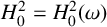$H^2_{0}=H^2_{0}(\omega )$ , $H^s=H^s(\gamma )$ ( $s=1/2, 3/2$ ).

The scalar products on $L^2$ and $H^2_0$ are denoted respectively by

$$ \begin{align*} (\eta,\varphi)_{0}&=\displaystyle\int_{\omega} \eta\varphi\,dx \quad\text{for all } \eta,\varphi\in L^2,\\ (\eta,\varphi)_{\Delta}&=(\Delta\eta,\Delta\varphi)_0\quad \text{for all } \eta,\varphi\in H_0^2, \end{align*} $$

with respective norms

$$ \begin{align*} \|\eta\|_{0}&=[(\eta,\eta)_{0}]^{1/2}\quad \text{for all } \eta \in L^2, \\ \|\eta\|_{\Delta}&=\|\Delta\eta\|_{0}\qquad\quad\text{for all } \eta \in H^2_0. \end{align*} $$

There exists a constant $\underline {\mu }>0$ such that

(3.1) $$ \begin{align} \|\eta\|_{0}\leq \underline{\mu}\|\eta\|_{\Delta}\quad \text{for all } \eta \in H^2_0. \end{align} $$

The dual spaces of $L^2$ and $H^2_0$ are denoted by $(L^2)^{\star }$ and $H^{-2}$ , respectively. The norm of $H^{-2}$ and the duality pairing between $H^{-2}$ and $H^2_0$ are denoted by $\|.\|_{-2}$ and $\langle .,.\rangle _{-2,2}$ , respectively. Also, the duality pairing between $(L^2)^{\star }$ and $L^2$ is denoted by $\langle .,.\rangle _{0}$ .

Let $G=(\Delta ^{2})^{-1}$ denote the Green operator of the Dirichlet problem for the biharmonic operator $\Delta ^{2}$ in $\omega $ . We note that the operator

(3.2) $$ \begin{align} \Delta^{2}: H^s\cap H_0^2 \longrightarrow H^{s-4}\quad\text{for }s\geq 2, \end{align} $$

is an isomorphism. Thus (see, for example, [Reference Chueshov and Lasiecka12, Remark 1.3.7]),

(3.3) $$ \begin{align} G \in \mathcal{L}(H^s;H^{s+4}\cap H_0^2) \quad\text{for }s\geq -2. \end{align} $$

In the following, we denote strong convergence by $\rightarrow $ and weak convergence by $\rightharpoonup $ .

We assume that

(3.4) $$ \begin{align} (\phi_{0},\phi_{1})\in H^{3/2}\times H^{1/2}. \end{align} $$

Then, by the classical elliptic theory [Reference Ciarlet14, page 395], there exists a unique function $\theta _{0}\in H^{2}$ which satisfies (2.3).

We also assume that

(3.5) $$ \begin{align} \theta\in H^{2}_{0} \end{align} $$

and

(3.6) $$ \begin{align} v\in L^{2}. \end{align} $$

The regularity condition $\theta \in H_{0}^{2}$ imposed in Sections 3 and 4 is appropriate for the well-posedness of the problem. In Sections 5 and 6, additional regularity is required to derive further properties.

We define the bilinear operator $B: H^{2}\times H^{2}\longrightarrow H_{0}^{2}$ as follows: for each pair $(\eta ,\varphi )\in H^{2}\times H^{2}$ , the function 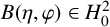$B(\eta ,\varphi )\in H_{0}^{2}$ is the unique solution to the problem:

$$ \begin{align*} \Delta ^{2}B(\eta,\varphi) =[\eta,\varphi] \quad\text{in }\omega. \end{align*} $$

Next, we define the cubic nonlinear operator 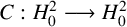${C}:H_{0}^{2}\longrightarrow H_{0}^{2}$ by

$$ \begin{align*} C({\eta})=B(B({\eta},{\eta}),{\eta}). \end{align*} $$

Then, we define the linear operators $L_{1}, L_{2} \in \mathcal {L}(H_{0}^{2};H_{0}^{2}) $ by

$$ \begin{align*} L_{1}({\eta})=B(B(\theta,\theta),\eta) \quad\text{and}\quad L_{2}(\eta)=B(\theta_{0},\eta). \end{align*} $$

In the following lemmas, we gather the properties of the operators G, B, C, $L_{1}$ and $L_{2}$ .

Lemma 3.1. The Green operator G satisfies the following estimate:

(3.7) $$ \begin{align} \|G\eta\|_{\Delta}\leq \underline{\mu}\|\eta\|_{0}\quad\text{for all } \eta \in L^2, \end{align} $$

where $\underline {\mu }$ is defined in (3.1).

Proof. For any $\eta \in L^2$ and $\varphi \in H_0^2$ ,

(3.8) $$ \begin{align} (G\eta,\varphi)_{\Delta}&=(\Delta G\eta,\Delta\varphi)_{0}\nonumber\\ &=(\eta,\varphi)_{0}. \end{align} $$

Then, by (3.1),

$$ \begin{align*} \|G\eta\|_{\Delta}^{2}&=(G\eta,G\eta)_{\Delta}\\ &=(\eta,G\eta)_{0}\\ &\leq \|\eta\|_{0}\|G\eta\|_{0}\\ &\leq \underline{\mu}\|\eta\|_{0}\|G\eta\|_{\Delta}. \end{align*} $$

This proves (3.7).

Lemma 3.2. If one of the arguments $\eta ,\varphi ,\psi $ belongs to $H_{0}^{2}$ , then

$$ \begin{align*} (B(\eta,\varphi),\psi)_{\Delta}=(B(\psi,\varphi),\eta)_{\Delta}. \end{align*} $$

Here, this property requires weaker assumptions imposed on three arguments than those imposed by Bock et al. [Reference Bock, Hlaváček and Lovíšek6, Proof of Lemma 4.1] (that all arguments are in $H^2_0$ ). In particular, this is needed to show (4.4), due to the presence of the function $\theta _{0}\in H^2$ , which solves (2.3).

Lemma 3.4. Let $(\eta ,\varphi )\in H_{0}^{2}\times H_{0}^{2}$ , then

$$ \begin{align*} (C(\eta)-C(\varphi),\varphi-\eta)_{\Delta} \leq\| B\|^{2}\max\{\|\eta\|^{2}_{\Delta},\|\varphi\|^{2}_{\Delta}\}\|\eta-\varphi\|^{2}_{\Delta}, \end{align*} $$

where

$$ \begin{align*} \|B\|=\displaystyle\sup_{\eta,\varphi\in H_{0}^{2},\|\eta\|=\|\varphi\|=1}\|B(\eta,\varphi)\|. \end{align*} $$

Proof. The continuity and compactness of operators $L_{1}$ and $L_{2}$ are immediately deduced from the properties of the operator B. The fact that $L_{2}$ is symmetric with respect to the inner product $(.,.)_{\Delta }$ was proved by Ciarlet [Reference Ciarlet14, Theorem 5.8-2(d)].

Let $\eta ,\varphi \in H_{0}^{2}$ . According to Lemma 3.2, we deduce that

$$ \begin{align*} (L_{1}(\eta),\varphi)_{\Delta}&=(B(B(\theta,\theta),\eta),\varphi)_{\Delta}\\ &=(B(B(\theta,\theta),\varphi),\eta)_{\Delta}\\ &=(L_{1}(\varphi),\eta)_{\Delta}. \end{align*} $$

Thus, $L_{1}$ is symmetric with respect to the inner product $(.,.)_{\Delta }$ .

4 Reduced Marguerre–von Kármán equation

4.1 Cubic operator equation

First, on the one hand, the definition of the bilinear operator B implies that the equations

$$ \begin{align*} \begin{cases} \Delta^2 \Phi =[\theta,\theta]-[\xi,\xi] &\text{in } \omega,\\ \Phi = \partial_{\nu}\Phi = 0 &\text{on } \gamma, \end{cases} \end{align*} $$

which are part of the canonical Marguerre–von Kármán equations (2.5), are equivalent to the operator equation in $H^{2}_{0}$ :

(4.1) $$ \begin{align} \Phi=B(\theta,\theta)-B(\xi,\xi). \end{align} $$

On the other hand, the definition of the bilinear operator B and that of the operator G imply that the remaining equations in the canonical Marguerre–von Kármán equations (2.5), namely

$$ \begin{align*} \begin{cases} \Delta^2\xi= [\Phi,\xi]+\lambda[\theta_{0},\xi] + v+\Delta ^2 \theta &\text{in } \omega,\\ \xi = \partial_{\nu}\xi = 0 &\text{on } \gamma, \end{cases} \end{align*} $$

are equivalent to the operator equation in $H^{2}_{0}$ :

(4.2) $$ \begin{align} \xi- G v-\theta=B(\Phi,\xi)+\lambda B(\theta_{0},\xi). \end{align} $$

Next, substituting (4.1) into (4.2) and using the bilinearity of the operator B, we derive the following single operator equation in $H^{2}_{0}$ :

$$ \begin{align*} \xi- G v-\theta=B(B(\theta,\theta),\xi)-B(B({\xi},{\xi}),{\xi})+\lambda B(\theta_{0},\xi). \end{align*} $$

From the definition of the operators C, $L_{1}$ and $L_{2}$ , we infer that the pair $(\xi ,\Phi )$ satisfies the canonical Marguerre–von Kármán equations (2.5) if and only if the unknown $\xi \in H^{2}_{0}$ satisfies the reduced Marguerre–von Kármán equation:

(4.3) $$ \begin{align} \xi- \lambda L_{2}(\xi)+C(\xi)-L_{1}(\xi)=G v+\theta, \end{align} $$

and the Airy function $\Phi \in H^{2}_{0}$ satisfies (4.1).

Therefore, we conclude that finding the solution $\xi $ to the operator equation (4.3) is equivalent to solving the following variational problem (see [Reference Bendob and Ghezal1]).

$$ \begin{align*} \begin{cases} \text{Find }\xi\in H^{2}_{0}\text{ such that}\\ (\xi- \lambda L_{2}(\xi)+C(\xi)-L_{1}(\xi)-G v-\theta,\eta)_{\Delta}=0 \quad\text{for all }\eta\in H^{2}_{0}. \end{cases} \end{align*} $$

4.2 General existence result

We consider the operator 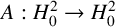$A: H_{0}^{2}\rightarrow H_{0}^{2}$ defined by

$$ \begin{align*} A=id_{H_{0}^{2}}-\lambda L_{2}+C-L_{1}. \end{align*} $$

Lemma 4.1. The operator A is coercive.

Proof. From the definition of the operators $L_{1},L_{2},C $ ,

$$ \begin{align*} (A(\xi),\xi)_{\Delta}= \| \xi\|^{2}_{\Delta}-\lambda(B(\theta _{0},\xi),\xi)_{\Delta}+ (B(B(\xi,\xi),\xi),\xi)_{\Delta}-(B(B(\theta,\theta),\xi),\xi)_{\Delta}. \end{align*} $$

According to Lemma 3.2,

(4.4) $$ \begin{align} (A(\xi),\xi)_{\Delta} = \| \xi\|^{2}_{\Delta}-\lambda( B(\xi,\xi),\theta _{0})_{\Delta}+ \| B(\xi,\xi)\|^{2}_{\Delta}-(B(\xi,\xi),B(\theta,\theta))_{\Delta}. \end{align} $$

By Cauchy–Schwarz inequality and Young’s inequality, we obtain

$$ \begin{align*} \begin{aligned} \lambda( B(\xi,\xi),\theta _{0})_{\Delta}&=( B(\xi,\xi),\lambda\theta _{0})_{\Delta} \\ & \leq \frac{1}{2}\| B(\xi,\xi)\|^{2}_{\Delta} +\frac{\lambda^{2}}{2}\|\theta _{0}\|^{2}_{\Delta} \end{aligned} \end{align*} $$

and

$$ \begin{align*} (B(\xi,\xi),B(\theta,\theta))_{\Delta}\leq \tfrac{1}{2}\| B(\xi,\xi)\|^{2}_{\Delta} + \tfrac{1}{2}\| B(\theta,\theta)\|^{2}_{\Delta}. \end{align*} $$

Consequently,

$$ \begin{align*} (A(\xi),\xi)_{\Delta} &\geq \|\xi\|^{2}_{\Delta} -\frac{1}{2}\| B(\xi,\xi)\|^{2}_{\Delta} -\frac{\lambda^{2}}{2}\|\theta _{0}\|^{2}_{\Delta}+ \| B(\xi,\xi)\|^{2}_{\Delta}-\frac{1}{2}\| B(\xi,\xi)\|^{2}_{\Delta} - \frac{1}{2}\| B(\theta,\theta)\|^{2}_{\Delta}\notag \\ &\geq\|\xi\|^{2}_{\Delta} -\frac{\lambda^{2}}{2}\|\theta _{0}\|^{2}_{\Delta} -\frac{1}{2}\| B(\theta,\theta)\|^{2}_{\Delta}. \end{align*} $$

Hence,

$$ \begin{align*} \dfrac{( A(\xi),\xi)_{\Delta}}{\|\xi\|_{\Delta}} \geq \|\xi\|_{\Delta} -\frac{\lambda^{2}}{2}\|\theta _{0}\|^{2}_{\Delta}\|\xi\|^{-1}_{\Delta} -\frac{1}{2}\| B(\theta,\theta)\|^{2}_{\Delta}\|\xi\|^{-1}_{\Delta}. \end{align*} $$

Since $\| A(\xi )\|_{\Delta }\geq ({( A(\xi ),\xi )_{\Delta }}/{\|\xi \|_{\Delta }})$ , we infer that

$$ \begin{align*} \lim_{\|\xi\|_{\Delta}\rightarrow \infty} \| A(\xi)\|_{\Delta}=\infty \end{align*} $$

for fixed $\lambda $ . This is the coerciveness of A. For details about these questions for von Kármán equation, see, for example, the paper by Berger [Reference Berger3].

Lemma 4.2. The operator A is pseudomonotone and bounded.

Proof. Since operators $L_{1}$ , $L_{2}$ and C are strongly continuous, thus operator A is a strongly continuous perturbation of the identity. According to Zeidler [Reference Zeidler40, Proposition 27.6(b)], A is pseudomonotone and bounded.

We give a general existence result for the reduced Marguerre–von Kármán equation.

Theorem 4.3. Under assumptions (3.4)–(3.6), the operator equation (4.3) has a solution for every fixed $\lambda $ .

Proof. From Lemmas 4.1 and 4.2, the operator A is coercive, pseudomonotone and bounded. Hence, the main theorem on pseudomonotone operators given by Zeidler [Reference Zeidler40, Theorem 27.A] (due to Brezis [Reference Brezis9]) shows that the operator equation $A(\xi )=G v+\theta $ has a solution.

Similar results were obtained for operator equation (4.3): for the case $\lambda>0$ , we refer to the work of Bendob and Ghezal [Reference Bendob and Ghezal1, Theorem 3.3]; for the case $\lambda =1$ , we refer to Rao [Reference Rao35, Theorem 2.3], Gratie [Reference Gratie21, Theorem 8] and Chueshov and Lasiecka [Reference Chueshov and Lasiecka12, Theorem 1.5.7], with different approaches. For the operator equation of von Kármán equations, see, for example, Berger [Reference Berger3, page 106] and Zeidler [Reference Zeidler39, Theorem 65.A].

4.3 Uniqueness result

We assume that the linear operators

(4.5) $$ \begin{align} L_{1}, L_{2} \text{ are positive definite}, \end{align} $$

(in the particular case (2.7), $L_{2}$ is positive definite [Reference Ciarlet14, Theorem 5.9-1]). We conclude that $L_{1}$ and $L_{2}$ have an infinite number of distinct eigenvalues $\beta _{k}>0$ and $\mu _{k}>0$ (each of finite multiplicity), respectively, such that

$$ \begin{align*} \cdots<\beta_{k}<\cdots<\beta_{2}<\beta_{1} \quad \text{with }\,\beta_{k}\to 0\,\text{ as }k\to \infty, \end{align*} $$

$$ \begin{align*} \cdots<\mu_{k}<\cdots<\mu_{2}<\mu_{1}\quad \text{with } \,\mu_{k}\to 0\, \text{ as }k\to \infty, \end{align*} $$

where

$$ \begin{align*} \beta_{1}&=\displaystyle\sup_{\eta\in H_{0}^{2},\eta\neq 0}\frac{(L_{1}\eta,\eta)_{\Delta}}{\|\eta\|^{2}_{\Delta}}, \quad \mu_{1}=\displaystyle\sup_{\eta\in H_{0}^{2},\eta\neq 0}\frac{(L_{2}\eta,\eta)_{\Delta}}{\|\eta\|^{2}_{\Delta}}. \end{align*} $$

The smallest characteristic values of the operator of $L_{1}$ and $L_{2}$ are given respectively by

(4.6) $$ \begin{align} \alpha_{1}&=\frac{1}{\beta_{1}}=\displaystyle\inf_{\eta\in H_{0}^{2},\eta\neq 0}\frac{\|\eta\|^{2}_{\Delta}}{(L_{1}\eta,\eta)_{\Delta}}, \end{align} $$

(4.7) $$ \begin{align} \lambda_{1}&=\frac{1}{\mu_{1}}=\displaystyle\inf_{\eta\in H_{0}^{2},\eta\neq 0}\frac{\|\eta\|^{2}_{\Delta}}{(L_{2}\eta,\eta)_{\Delta}}. \end{align} $$

To give the uniqueness of solutions to reduced Marguerre–von Kármán equations, we need the following additional assumptions:

(4.8) $$ \begin{align} \|Gv+\theta\|_{\Delta}<\|B\|^{-1}, \end{align} $$

(4.9) $$ \begin{align} \alpha_{1}>\alpha^{\star}, \end{align} $$

(4.10) $$ \begin{align} \lambda<\lambda^{\star}, \end{align} $$

where

$$ \begin{align*} \alpha^{\star}=(1-\|B\|^{2/3}\|Gv+\theta\|_{\Delta}^{2/3})^{-1},\quad \lambda^{\star}=\lambda_{1}\bigg(1-\frac{1}{\alpha_{1}}-\|B\|^{2/3}\|Gv+\theta\|_{\Delta}^{2/3}\bigg). \end{align*} $$

Theorem 4.4. Under assumptions (3.4)–(3.6), (4.5) and (4.8)–(4.10), there exists a unique solution $\xi \in H^{2}_{0}$ to operator equation (4.3). Moreover, $\xi $ satisfies the estimate

(4.11) $$ \begin{align} \|\xi\|_{\Delta}\leq K(\lambda)^{-1}\|Gv+\theta\|_{\Delta}, \end{align} $$

where

(4.12) $$ \begin{align} K(\lambda)=\min\bigg\{1-\frac{1}{\alpha_{1}},1-\frac{1}{\alpha_{1}}-\frac{\lambda}{\lambda_{1}}\bigg\}>0. \end{align} $$

Proof.

1. (i) First, the existence of solutions $\xi \in H^{2}_{0}$ to operator equation (4.3) is verified in Theorem 4.3.

2. (ii) Let $\xi \in H^{2}_{0}$ be a solution to (4.3). Then,

   $$ \begin{align*} (\xi- \lambda L_{2}(\xi)+C(\xi)-L_{1}(\xi)-G v-\theta,\,\xi)_{\Delta}=0, \end{align*} $$
   and hence,
   $$ \begin{align*} \|\xi\|_{\Delta}^{2}-\lambda(L_{2}(\xi),\xi)_{\Delta}+(C(\xi),\xi)_{\Delta}-(L_{1}(\xi),\xi)_{\Delta}=(G v+\theta,\xi)_{\Delta}. \end{align*} $$
   According to Lemma 3.3, we deduce that
   (4.13) $$ \begin{align} \|\xi\|_{\Delta}^{2}-\lambda(L_{2}(\xi),\xi)_{\Delta}-(L_{1}(\xi),\xi)_{\Delta}\leq(G v+\theta,\xi)_{\Delta}. \end{align} $$

3. (iii) If $\lambda>0$ , then from the positivity of operators $L_{1}$ and $L_{2}$ , and relations (4.6)–(4.7),

   $$ \begin{align*} -\bigg(\frac{\lambda}{\lambda_{1}}+\frac{1}{\alpha_{1}}\bigg)\|\xi\|_{\Delta}^{2}\leq-\lambda(L_{2}(\xi),\xi)_{\Delta}-(L_{1}(\xi),\xi)_{\Delta}. \end{align*} $$
   We infer that
   $$ \begin{align*} \bigg(1-\frac{1}{\alpha_{1}}-\frac{\lambda}{\lambda_{1}}\bigg)\|\xi\|_{\Delta}^{2}\leq\|G v+\theta\|_{\Delta}\|\xi\|_{\Delta}. \end{align*} $$
   For $\lambda <\lambda _{1}(1-{1}/{\alpha _{1}})$ , we get
   (4.14) $$ \begin{align} \|\xi\|_{\Delta}\leq \bigg(1-\frac{1}{\alpha_{1}}-\frac{\lambda}{\lambda_{1}}\bigg)^{-1}\|Gv+\theta\|_{\Delta}. \end{align} $$
   Let $\xi _{1}$ and $\xi _{2}$ be two solutions of (4.3). Then,
   $$ \begin{align*} (id_{H_{0}^{2}}-\lambda L_{2}-L_{1})(\xi_{1}-\xi_{2})=C(\xi_{2})-C(\xi_{1}). \end{align*} $$
   Hence,
   $$ \begin{align*} ((id_{H_{0}^{2}}-\lambda L_{2}-L_{1})(\xi_{1}-\xi_{2}),\xi_{1}-\xi_{2})_{\Delta}=(C(\xi_{2})-C(\xi_{1}),\xi_{1}-\xi_{2})_{\Delta}. \end{align*} $$
   Applying Lemma 3.4,
   (4.15) $$ \begin{align} \bigg(1-\frac{1}{\alpha_{1}}-\frac{\lambda}{\lambda_{1}}\bigg)\|\xi_{1}-\xi_{2}\|_{\Delta}^{2}\leq \| B\|^{2}\max\{\|\xi_{1}\|^{2}_{\Delta},\|\xi_{2}\|^{2}_{\Delta}\}\|\xi_{2}-\xi_{1}\|^{2}_{\Delta}. \end{align} $$
   For $\lambda <\lambda _{1}(1-{1}/{\alpha _{1}})$ and by (4.14),
   $$ \begin{align*} \|\xi_{1}-\xi_{2}\|_{\Delta}^{2}\leq \bigg(1-\frac{1}{\alpha_{1}}-\frac{\lambda}{\lambda_{1}}\bigg)^{-3}\| B\|^{2}\|Gv+\theta\|_{\Delta}^{2}\|\xi_{1}-\xi_{2}\|^{2}_{\Delta}. \end{align*} $$
   By assumptions (4.9) and (4.10), we have that this inequality can be true only if $\xi _{1}=\xi _{2}$ .

4. (iv) If $\lambda \leq 0$ , then from (4.13) and the positivity of operator $L_{2}$ ,

   $$ \begin{align*} \|\xi\|_{\Delta}^{2}-(L_{1}(\xi),\xi)_{\Delta}\leq(G v+\theta,\xi)_{\Delta}. \end{align*} $$
   From the positivity of operators $L_{1}$ and relation (4.6),
   $$ \begin{align*} -\frac{1}{\alpha_{1}}\|\xi\|_{\Delta}^{2}\le -(L_{1}(\xi),\xi)_{\Delta}. \end{align*} $$
   We infer that
   $$ \begin{align*} \bigg(1-\frac{1}{\alpha_{1}}\bigg)\|\xi\|_{\Delta}\leq\|G v+\theta\|_{\Delta}. \end{align*} $$
   For $ \alpha _{1}>1$ ,
   (4.16) $$ \begin{align} \|\xi\|_{\Delta}\leq \bigg(1-\frac{1}{\alpha_{1}}\bigg)^{-1}\|Gv+\theta\|_{\Delta}. \end{align} $$
   Let $\xi _{1}$ and $\xi _{2}$ be two solutions of (4.3). Taking into account (4.15), we conclude that
   $$ \begin{align*} \bigg(1-\frac{1}{\alpha_{1}}\bigg)\|\xi_{1}-\xi_{2}\|_{\Delta}^{2}\leq \| B\|^{2}\max\{\|\xi_{1}\|^{2}_{\Delta},\|\xi_{2}\|^{2}_{\Delta}\}\|\xi_{2}-\xi_{1}\|^{2}_{\Delta}. \end{align*} $$
   For $ \alpha _{1}>1$ and by (4.16),
   $$ \begin{align*} \|\xi_{1}-\xi_{2}\|_{\Delta}^{2}\leq \bigg(1-\frac{1}{\alpha_{1}}\bigg)^{-3}\| B\|^{2}\|Gv+\theta\|_{\Delta}^{2}\|\xi_{1}-\xi_{2}\|^{2}_{\Delta}. \end{align*} $$
   By assumptions (4.8) and (4.9), we have that this inequality can be true only if $\xi _{1}=\xi _{2}$ .

5. (v) From assumptions (4.8)–(4.10),

   $$ \begin{align*} \alpha_{1}>\alpha^{\star}>1 \quad \text{and} \quad \lambda<\lambda^{\star}<\lambda_{1}\bigg(1-\frac{1}{\alpha_{1}}\bigg). \end{align*} $$
   Hence,
   $$ \begin{align*} 1-\frac{1}{\alpha_{1}}>0 \quad \text{and} \quad 1-\frac{1}{\alpha_{1}}-\frac{\lambda}{\lambda_{1}}>0. \end{align*} $$
   We infer that $K(\lambda )>0.$ Finally, using estimates (4.14) and (4.16) yields the desired result (4.11).

5 Existence of an optimal control for Marguerre–von Kármán equations

We follow a similar approach to (4.1) and (4.3). By replacing $(\xi ,\Phi )$ by $(\xi (v),\Phi (v))$ , we deduce that the pair $(\xi (v),\Phi (v))$ satisfies the control problem (2.9) if and only if $\xi (v)\in H^{2}_{0}$ satisfies the reduced equation:

(5.1) $$ \begin{align} \xi(v)- \lambda L_{2}(\xi(v))+C(\xi(v))-L_{1}(\xi(v))=Gv+\theta. \end{align} $$

The Airy function $\Phi (v)\in H^{2}_{0}$ is then given by

$$ \begin{align*} \Phi(v)=B(\theta,\theta)-B(\xi(v),\xi(v)). \end{align*} $$

Here, $\theta \in H^{2}_{0}$ and v belongs to the set of admissible controls $\mathcal {V}_{ad}$ , defined as

$$ \begin{align*} \mathcal{V}_{ad}=\{v\in L^{2}| \,\text{equation } (5.1) \text{ has a unique solution }\xi(v)\}. \end{align*} $$

We adopt the same general framework of the cost functional as presented by Bock et al. [Reference Bock, Hlaváček and Lovíšek6] (also see [Reference Bock, Hlaváček and Lovíšek7]). Therefore, the cost functional corresponding to state equation (5.1) is given by

(5.2) $$ \begin{align} \mathcal{J}(v)=J(\xi(v))+j(v),\quad v\in \mathcal{V}_{ad}, \end{align} $$

where the functionals, $J: L^2\longrightarrow \mathbb {R}$ is a state-dependent cost and 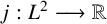$j: L^2\longrightarrow \mathbb {R}$ is a control-dependent cost, are certain functionals.

Let $v^* \in \mathcal {V}_{ad}$ be an optimal control for cost functional (5.2), that is,

$$ \begin{align*} \mathcal{J}(v^*) = \inf_{v \in \mathcal{V}_{ad}} \mathcal{J}(v). \end{align*} $$

According to Theorem 4.4, there exists a unique solution $\xi (v)\in H^{2}_{0}$ to state equation (5.1) for $\lambda <\lambda ^{\star }$ . This solution satisfies

$$ \begin{align*} \|\xi(v)\|_{\Delta}\leq K(\lambda)^{-1}\|Gv+\theta\|_{\Delta}. \end{align*} $$

We need the following additional assumption on $\theta $ :

(5.3) $$ \begin{align} \theta\in H^4\cap H_0^2, \end{align} $$

and hence by (3.2), we have $\Delta ^{2}\theta \in L^{2}$ .

We let

$$ \begin{align*} \mathcal{V}_{ad}=\bigg\{v\in L^{2}\bigg| \, \|v+\Delta^{2}\theta\|_{0}\leq \frac{\overline{\mu}}{\underline{\mu}}\|B\|^{-1}K(\lambda)^{3/2}\bigg\}, \end{align*} $$

where

(5.4) $$ \begin{align} 0<\overline{\mu}<1 \end{align} $$

is an arbitrary parameter, with $\lambda <\lambda _{1}(1-{1}/{\alpha _{1}})$ and $\alpha _{1}>1$ .

However, by using Lemma 3.1, if $v\in \mathcal {V}_{ad}$ , we infer that

(5.5) $$ \begin{align} \|Gv+\theta\|_{\Delta}=\|G(v+\Delta^{2}\theta)\|_{\Delta}\leq \overline{\mu}\|B\|^{-1}K(\lambda)^{3/2}, \end{align} $$

and thus assumptions (4.8)–(4.10) are valid. Hence, for every $v\in \mathcal {V}_{ad}$ , there exists a unique solution $\xi (v)\in H^{2}_{0}$ to state equation (5.1).

Now, we prove the existence theorem for the following optimal control problem.

(5.6) $$ \begin{align} \begin{cases} \text{Find } v^*\in \mathcal{V}_{ad}\text{ such that} \\ \mathcal{J}(v^*) = \displaystyle\inf_{v \in \mathcal{V}_{ad}} \mathcal{J}(v),\\ \xi(v^*)- \lambda L_{2}(\xi(v^*))+C(\xi(v^*))-L_{1}(\xi(v^*))=Gv^*+\theta. \end{cases} \end{align} $$

Proof. Using the same idea as in [Reference Bock, Hlaváček and Lovíšek6, the proof of Theorem 3.1], we deduce the existence of a minimizing sequence $\{v_{n}\}\subset \mathcal {V}_{ad}$ , that is,

$$ \begin{align*} \displaystyle\lim\limits_{n\to+\infty}\mathcal{J}(v_{n})=\inf_{v \in \mathcal{V}_{ad}} \mathcal{J}(v). \end{align*} $$

It is clear that $\mathcal {V}_{ad}$ is bounded in $L^{2}$ and that $\mathcal {V}_{ad}$ (closed and convex) is weakly sequentially closed in $L^{2}$ . Therefore, there exists a subsequence, still denoted by $\{v_n\}$ , which converges weakly in $L^{2}$ :

$$ \begin{align*} v_n \rightharpoonup v^* \text{ in } L^{2} \quad\text{as }n \to \infty, \quad v^*\in\mathcal{V}_{ad}. \end{align*} $$

From (4.11), (5.5), we obtain the following estimate of all states:

(5.7) $$ \begin{align} \|\xi(v)\|_{\Delta}\leq \overline{\mu}\|B\|^{-1}K(\lambda)^{1/2} \quad \text{for all } v\in \mathcal{V}_{ad}. \end{align} $$

This implies that $\{\xi (v_n)\}$ is bounded in $H^{2}_{0}$ . We can find a subsequence, still denoted by $\{v_n\}$ , such that

$$ \begin{align*} \xi_n \rightharpoonup \xi^* \text{ in } H^{2}_{0} \quad\text{as }n \to \infty, \quad \xi_n=\xi(v_n), \end{align*} $$

and

(5.8) $$ \begin{align} \xi_n- \lambda L_{2}(\xi_n)+C(\xi_n)-L_{1}(\xi_n)=Gv_n+\theta. \end{align} $$

According to Lemmas 3.3 and 3.5, we see that the nonlinear operator C is sequentially compact and the linear operators $L_{1}$ and $L_{2}$ are compact. Thus, we obtain the following strong convergences:

$$ \begin{align*} C(\xi_n)&\rightarrow C(\xi^*)\text{ in } H^{2}_{0} \quad\text{as }n \to \infty,\\ L_{1}(\xi_n)&\rightarrow L_{1}(\xi^*) \text{ in } H^{2}_{0} \quad\text{as }n \to \infty,\\ L_{2}(\xi_n)&\rightarrow L_{2}(\xi^*)\text{ in } H^{2}_{0} \quad\text{as }n \to \infty. \end{align*} $$

Using (3.3) gives

$$ \begin{align*} Gv_n \rightharpoonup Gv^* \text{ in } H^{4}\cap H_0^2 \quad\text{as }n \to \infty. \end{align*} $$

Passing to a weak limit in (5.8),

$$ \begin{align*} \xi^*- \lambda L_{2}(\xi^*)+C(\xi^*)-L_{1}(\xi^*)=Gv^*+\theta. \end{align*} $$

From the uniqueness of the solution to state equation (5.1),

$$ \begin{align*} \xi_n \rightharpoonup \xi(v^*) \text{ in } H^{2}_{0} \quad\text{as }n \to \infty, \quad \xi^*=\xi(v^*). \end{align*} $$

The weak lower semicontinuity of J and j gives

$$ \begin{align*} \mathcal{J}(v^*)&=J(\xi(v^*))+j(v^*)\\ &\leq \liminf_{n\to\infty}J(\xi(v_n))+\liminf_{n\to\infty}j(v_n)\\ &\leq\liminf_{n\to\infty}\mathcal{J}(v_n)\\ &=\inf_{v \in \mathcal{V}_{ad}} \mathcal{J}(v). \end{align*} $$

This concludes the proof.

6 Characterization of the optimal control

Our goal in this section is to prove the uniqueness of the optimal control and derive the necessary optimality condition, by using the Fréchet differentiability.

6.1 Differentiability of the state function

Later on (see Theorem 6.2), we show that the mapping

$$ \begin{align*} \xi(.): \mathcal{V}_{ad} \longrightarrow H^{2}_{0}, \end{align*} $$

defined by state equation (5.1), is Fréchet differentiable.

We also show that the derivative

$$ \begin{align*} \xi^{\prime}(v): L^{2} \longrightarrow H^{2}_{0} \end{align*} $$

is determined by the solution of the equation:

(6.1) $$ \begin{align} [id_{H_{0}^{2}}-\lambda L_{2}+C^{\prime}(\xi(v))-L_{1}]\xi^{\prime}(v)h=Gh, \quad h\in L^{2}, \end{align} $$

where

(6.2) $$ \begin{align} C^{\prime}(\xi)\eta=2B(B(\xi,\eta),\xi)+B(B(\xi,\xi),\eta), \quad \xi,\eta\in H^{2}_{0}. \end{align} $$

Here, $C^{\prime }(\xi )\in \mathcal {L}(H^{2}_{0};H^{1}_{0})$ is the Gâteaux derivative of the operator C at the point $\xi \in H^{2}_{0}$ (see, for example, [Reference Ciarlet and Rabier18, page 90]).

We consider the operator $\mathcal {A}(\xi (v)): H_{0}^{2}\longrightarrow H_{0}^{2}$ defined by

(6.3) $$ \begin{align} \mathcal{A}(\xi(v))=id_{H_{0}^{2}}-\lambda L_{2}+C^{\prime}(\xi(v))-L_{1}. \end{align} $$

Lemma 6.1. The operator $A(\xi (v))$ is linear, positive definite and symmetric with respect to the inner product $(.,.)_{\Delta }$ .

Proof. It is easy to see from the properties of operators B, $L_{1}$ and $L_{2}$ described in the statement of Lemmas 3.2 and 3.5 and relation (6.2) that the operator $A(\xi (v))$ is linear and symmetric.

For all $\eta \in H^{2}_{0}$ ,

$$ \begin{align*} (\mathcal{A}(\xi(v))\eta,\eta)_{\Delta}&=\| \eta\|^{2}_{\Delta}-\lambda(L_{2}\eta,\eta)_{\Delta}+2(B(B(\xi(v),\eta),\xi(v)),\eta)_{\Delta}\\ &\quad +(B(B(\xi(v),\xi(v)),\eta),\eta)_{\Delta}-(L_{1}\eta,\eta)_{\Delta}. \end{align*} $$

Using Lemma 3.2,

$$ \begin{align*} (\mathcal{A}(\xi(v))\eta,\eta)_{\Delta}&=\| \eta\|^{2}_{\Delta}-\lambda(L_{2}\eta,\eta)_{\Delta}+2(B(\xi(v),\eta),B(\xi(v),\eta))_{\Delta}\\ &\quad +(B(\xi(v),\xi(v)),B(\eta,\eta))_{\Delta}-(L_{1}\eta,\eta)_{\Delta}\\ &=\| \eta\|^{2}_{\Delta}-\lambda(L_{2}\eta,\eta)_{\Delta}+2\|B(\xi(v),\eta)\|^{2}_{\Delta}\\ &\quad +(B(\xi(v),\xi(v)),B(\eta,\eta))_{\Delta}-(L_{1}\eta,\eta)_{\Delta}. \end{align*} $$

Therefore, as in the proof of Theorem 4.4,

$$ \begin{align*} (\mathcal{A}(\xi(v))\eta,\eta)_{\Delta}&\geq K(\lambda)\|\eta\|^{2}_{\Delta}-\|B\|^{2}\|\xi(v)\|^{2}_{\Delta}\|\eta\|^{2}_{\Delta}. \end{align*} $$

Then, using (5.7) gives

$$ \begin{align*} (A(\xi(v))\eta,\eta)_{\Delta}&\geq (1-\overline{\mu}^{2})K(\lambda)\|\eta\|^{2}_{\Delta}. \end{align*} $$

Finally, we set

$$ \begin{align*} \overline{K}(\lambda)=(1-\overline{\mu}^{2})K(\lambda). \end{align*} $$

Moreover, one can easily see from (4.12) and (5.4) that

$$ \begin{align*} \overline{K}(\lambda)>0. \end{align*} $$

Hence,

(6.4) $$ \begin{align} (\mathcal{A}(\xi(v))\eta,\eta)_{\Delta}\geq \overline{K}(\lambda)\|\eta\|^{2}_{\Delta}. \end{align} $$

This proves the positive definiteness of $A(\xi (v))$ .

Theorem 6.2. The mapping $\xi (.)$ determined by state equation (5.1) is Fréchet differentiable with respect to $v\in \mathring {\mathcal {V}}_{ad}$ ( $\mathring {\mathcal {V}}_{ad}$ denotes the interior of $\mathcal {V}_{ad}$ ) and $\xi ^{\prime }(v)$ satisfies equation (6.1) for all $h\in L^{2}$ .

Proof. As a result of Lemma 6.1, there exists a unique solution $\varphi (h)$ of the equation

(6.5) $$ \begin{align} \mathcal{A}(\xi(v))\varphi(h)=[id_{H_{0}^{2}}-\lambda L_{2}+C^{\prime}(\xi(v))-L_{1}]\varphi(h)=Gh \quad\text{for all } h\in L^{2}. \end{align} $$

Let

$$ \begin{align*} \psi=\psi(h)=\widetilde{\xi}-\varphi(h), \end{align*} $$

where

(6.6) $$ \begin{align} \widetilde{\xi}=\xi(v+h)-\xi(v); \quad v,\, v+h\in\mathcal{V}_{ad}. \end{align} $$

To establish that $ \varphi (h)=\xi ^{\prime }(v)h$ is the differential of $\xi $ in the sense of Fréchet, it is sufficient to verify that

(6.7) $$ \begin{align} \|\psi\|_{\Delta}=o(h). \end{align} $$

By using state equation (5.1) and (6.5),

(6.8) $$ \begin{align} \mathcal{A}(\xi(v))\psi&=[id_{H_{0}^{2}}-\lambda L_{2}+C^{\prime}(\xi(v))-L_{1}]\psi\nonumber\\ &=[id_{H_{0}^{2}}-\lambda L_{2}-L_{1}](\xi(v+h)-\xi(v)) +C^{\prime}(\xi(v))(\xi(v+h)-\xi(v))\nonumber\\ &\quad -[id_{H_{0}^{2}}-\lambda L_{2}+C^{\prime}(\xi(v))-L_{1}]\varphi(h)\nonumber\\ &=G(v+h)-C(\xi(v+h))-G(v)+C(\xi(v))\nonumber\\ &\quad+C^{\prime}(\xi(v))(\xi(v+h)-\xi(v))-Gh\nonumber\\ &=C^{\prime}(\xi(v))(\xi(v+h)-\xi(v))-[C(\xi(v+h))-C(\xi(v))] \notag\\ &=\displaystyle\int_{0}^{1}[C^{\prime}(\xi(v))-C^{\prime}(\xi(v)+s\widetilde{\xi}) ]\widetilde{\xi}\,ds. \end{align} $$

Moreover, because of the positive definiteness of $\mathcal {A}(\xi (v))$ , there exists $C(\lambda )>0$ such that

(6.9) $$ \begin{align} \|\psi\|_{\Delta}\leq C(\lambda)\|\widetilde{\xi}\|_{\Delta}^{2}. \end{align} $$

From (6.5) and (6.8),

$$ \begin{align*} \mathcal{A}(\xi(v))\varphi(h)&=[id_{H_{0}^{2}}-\lambda L_{2}+C^{\prime}(\xi(v))-L_{1}](\xi(v+h)-\xi(v)-\psi) \\ &=[id_{H_{0}^{2}}-\lambda L_{2}-L_{1}](\xi(v+h)-\xi(v)) +C^{\prime}(\xi(v))(\xi(v+h)-\xi(v)) \\ &\quad -[id_{H_{0}^{2}}-\lambda L_{2}+C^{\prime}(\xi(v))-L_{1}]\psi \\ &=[id_{H_{0}^{2}}-\lambda L_{2}-L_{1}](\xi(v+h)-\xi(v)) +C^{\prime}(\xi(v))(\xi(v+h)-\xi(v)) \\ &\quad -C^{\prime}(\xi(v))(\xi(v+h)-\xi(v))+[C(\xi(v+h))-C(\xi(v))] \\ &=[id_{H_{0}^{2}}-\lambda L_{2}-L_{1}]\widetilde{\xi}+C(\xi(v+h))-C(\xi(v)). \end{align*} $$

Then, the function $\widetilde {\xi }$ satisfies

$$ \begin{align*} \widetilde{\xi}- \lambda L_{2}(\widetilde{\xi})-L_{1}(\widetilde{\xi})+C(\xi(v+h))-C(\xi(v))=Gh. \end{align*} $$

By virtue of Lemmas 3.1 and 3.4,

$$ \begin{align*} K(\lambda)\|\widetilde{\xi}\|_{\Delta}^{2} - \| B\|^{2}\max\{\|\xi(v)\|^{2}_{\Delta},\|\xi(v+h)\|^{2}_{\Delta}\}\|\widetilde{\xi}\|^{2}_{\Delta}\leq \underline{\mu}\|h\|_{0}\|\widetilde{\xi}\|_{\Delta}. \end{align*} $$

Taking into account estimate (5.7),

(6.10) $$ \begin{align} \|\widetilde{\xi}\|_{\Delta}\leq \underline{K}(\lambda)\|h\|_{0}, \end{align} $$

where

$$ \begin{align*} \underline{K}(\lambda)=\underline{\mu}\overline{K}(\lambda)^{-1}. \end{align*} $$

Using (6.6), (6.9) and (6.10),

$$ \begin{align*} \|\psi\|_{\Delta}=\|\xi(v+h)-\xi(v)-\varphi(h)\|_{\Delta}=o(h), \end{align*} $$

and hence (6.7) is verified.

6.2 Uniqueness of the optimal control

Let us assume that the functional J and j are Fréchet differentiable. Because we have shown in Theorem 6.2 that the mapping $\xi (.)$ determined by state equation (5.1) is Fréchet differentiable at the optimal control $v^*$ , we infer that the functional $\mathcal {J}$ is also Fréchet differentiable at $v^*$ such that

$$ \begin{align*} \langle \mathcal{J}^{\prime}(v^*),v\rangle_{0}=\langle J^{\prime}(\xi(v^*)),\xi^{\prime}(v^*)v\rangle_{-2,2}+\langle j^{\prime}(v^*),v\rangle_{0} \quad \text{for all } v\in \mathcal{V}_{ad}. \end{align*} $$

Similar to the case of optimal control problems governed by von Kármán equations presented by Bock et al. [Reference Bock, Hlaváček and Lovíšek6] (also see [Reference Bock, Hlaváček and Lovíšek7]), assume that the derivatives $J^{\prime }$ and $j^{\prime }$ satisfy the following conditions:

(6.11) $$ \begin{align} \langle J^{\prime}(\xi_{1})-J^{\prime}(\xi_{2}),\xi_{1}-\xi_{2}\rangle_{-2,2}\geq \sigma\|\xi_{1}-\xi_{2}\|_{\Delta}^{2}\quad \text{for all } \xi_{1},\xi_{2}\in H^{2}_{0}, \end{align} $$

(6.12) $$ \begin{align} \langle j^{\prime}(v_{1})-j^{\prime}(v_{2}),v_{1}-v_{2}\rangle_{0}\geq \rho\|v_{1}-v_{2} \|_{0}^{2}\quad \text{for all } v_{1},v_{2}\in L^{2}, \end{align} $$

where $\sigma $ and $\rho $ are positive constants.

Also, the derivative $J^{\prime }$ satisfies the following condition:

(6.13) $$ \begin{align} \|J^{\prime}(\xi)\|_{-2}\leq\kappa_{1}\|\xi\|_{\Delta}+\kappa_{2}, \end{align} $$

where $\kappa _{1}>0$ and $\kappa _{2}$ are some constants.

The technical conditions (6.11)–(6.13) assert that the derivatives $J^{\prime }$ and $j^{\prime }$ are strongly monotone and $J^{\prime }$ grows at most linearly with $\xi $ . The conditions (6.11) and (6.12) are common in monotone operator theory [Reference Zeidler40], and (6.13) is standard in control theory for PDEs [Reference Lions29, Reference Tröltzsch36]. These conditions play a critical role in the following uniqueness result.

Theorem 6.3. Let the assumptions of Theorem 5.1 and (6.11)–(6.13) be valid. If

$$ \begin{align*} \rho>\{-\sigma+6\overline{\mu}\overline{K}(\lambda)^{-1}K(\lambda)^{1/2}\|B\|(\kappa_{1}\overline{\mu}\|B\|^{-1}K(\lambda)^{1/2}+\kappa_{2}) \}\underline{K}(\lambda)^{2}, \end{align*} $$

then there exists a unique solution $v^*$ of problem (5.6).

Proof. If $v^*\in \mathcal {V}_{ad}$ is a solution to problem (5.6) ( $v^*$ is the optimal control), then

$$ \begin{align*} \langle \mathcal{J}^{\prime}(v^*),v-v^*\rangle_{0}\geq 0\quad\text{for all } v\in \mathcal{V}_{ad}. \end{align*} $$

Let 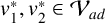$v^*_{1}, v^*_{2}\in \mathcal {V}_{ad}$ be two solutions to problem (5.6), then

(6.14) $$ \begin{align} \kern1.5pt\langle \mathcal{J}^{\prime}(v^*_{1}),v-v^*_{1}\rangle_{0}&=\langle J^{\prime}(\xi(v^*_{1})),\xi^{\prime}(v^*_{1})(v-v^*_{1})\rangle_{-2,2}+\langle j^{\prime}(v^*_{1}),v-v^*_{1}\rangle_{0}\geq 0, \end{align} $$

(6.15) $$ \begin{align} \langle \mathcal{J}^{\prime}(v^*_{2}),v-v^*_{2}\rangle_{0}&=\langle J^{\prime}(\xi(v^*_{2})),\xi^{\prime}(v^*_{2})(v-v^*_{2})\rangle_{-2,2}+\langle j^{\prime}(v^*_{2}),v-v^*_{2}\rangle_{0}\geq 0 \end{align} $$

for all $v\in \mathcal {V}_{ad}$ .

Taking $v=v^*_{2}$ in (6.14), $v=v^*_{1}$ in (6.15) and adding,

$$ \begin{align*} &\langle J^{\prime}(\xi(v^*_{1}))-J^{\prime}(\xi(v^*_{2})),\xi(v^*_{2})-\xi(v^*_{1})\rangle_{-2,2}+\langle j^{\prime}(v^*_{1})-j^{\prime}(v^*_{2}),v^*_{2}-v^*_{1}\rangle_{0}\nonumber\\ &\quad-\langle J^{\prime}(\xi(v^*_{1})),\xi(v^*_{2})-\xi(v^*_{1})-\xi^{\prime}(v^*_{1})(v^*_{2}-v^*_{1}) \rangle_{-2,2}\nonumber\\ &\quad-\langle J^{\prime}(\xi(v^*_{2})),\xi(v^*_{1})-\xi(v^*_{2})-\xi^{\prime}(v^*_{2})(v^*_{1}-v^*_{2}) \rangle_{-2,2}\geq 0. \end{align*} $$

We set

(6.16) $$ \begin{align} \psi_{1}&=\xi(v^*_{2})-\xi(v^*_{1})-\xi^{\prime}(v^*_{1})(v^*_{2}-v^*_{1}), \end{align} $$

(6.17) $$ \begin{align} \psi_{2}&=\xi(v^*_{1})-\xi(v^*_{2})-\xi^{\prime}(v^*_{2})(v^*_{1}-v^*_{2}), \end{align} $$

(6.18) $$ \begin{align} \widehat{\xi}&=\xi(v^*_{2})-\xi(v^*_{1}). \qquad\qquad\qquad \end{align} $$

By assumptions (6.11)–(6.12) and relations (6.16)–(6.18),

(6.19) $$ \begin{align} -\sigma\|\widehat{\xi}\|_{\Delta}^{2} -\rho\|v^*_{1}-v^*_{2} \|_{0}^{2} -\langle J^{\prime}(\xi(v^*_{1})),\psi_{1} \rangle_{-2,2}-\langle J^{\prime}(\xi(v^*_{2})),\psi_{2} \rangle_{-2,2}\geq 0. \end{align} $$

To estimate $\psi _{1}$ , with similar computations for estimate (6.9), readily

(6.20) $$ \begin{align} [id_{H_{0}^{2}}-\lambda L_{2}+C^{\prime}(\xi(v^*_{1}))-L_{1}]\psi_{1}&=C^{\prime}(\xi(v^*_{1}))(\xi(v^*_{2})-\xi(v^*_{1}))+C(\xi(v^*_{1}))-C(\xi(v^*_{2}))\nonumber\\ &=\displaystyle\int_{0}^{1}[C^{\prime}(\xi(v^*_{1}))-C^{\prime}(\xi(v^*_{1})+s\widehat{\xi}) ]\widehat{\xi}\, ds\nonumber\\ &=\Psi. \end{align} $$

The mean value theorem implies

$$ \begin{align*} \|\Psi\|_{\Delta}&=\sup_{\|h\|_{\Delta}=1}\bigg|\bigg(\displaystyle\int_{0}^{1}[C^{\prime}(\xi(v^*_{1}))-C^{\prime}(\xi(v^*_{1})+s\widehat{\xi}) ]\widehat{\xi}\, ds,h\bigg)_{\Delta}\bigg|\\ &=\sup_{\|h\|_{\Delta}=1}\bigg|\bigg(\displaystyle\int_{0}^{1}C^{\prime\prime}(\xi(v^*_{1})+\tau(s)\widehat{\xi})(\widetilde{\xi},\widetilde{\xi})s\, ds,h\bigg)_{\Delta}\bigg|, \end{align*} $$

where $\tau (s)\in (0,s)$ and the second derivative $C^{\prime \prime }$ has the form

$$ \begin{align*} C^{\prime\prime}(\xi)(\widehat{\xi},\widehat{\xi})=2B(B(\widehat{\xi},\widehat{\xi}),\xi)+4B(B(\xi,\widehat{\xi}),\widehat{\xi})\quad \text{for all } \xi,\widehat{\xi}\in H^{2}_{0}. \end{align*} $$

Using estimate (5.7),

(6.21) $$ \begin{align} \|\Psi\|_{\Delta}\leq 3\overline{\mu}K(\lambda)^{1/2}\|B\|\|\widehat{\xi}\|_{\Delta}^{2}. \end{align} $$

From the positive definiteness of $A(\xi (v))$ in (6.4), and relations (6.20) and (6.21),

(6.22) $$ \begin{align} \|\psi_{1}\|_{\Delta}\leq 3\overline{\mu}\overline{K}(\lambda)^{-1}K(\lambda)^{1/2}\|B\|\|\widehat{\xi}\|_{\Delta}^{2}, \end{align} $$

and similarly for $\psi _{2}$ .

By assumption (6.13), relations (5.7), (6.19) and (6.22),

(6.23) $$ \begin{align} \{-\sigma+6\overline{\mu}\overline{K}(\lambda)^{-1}K(\lambda)^{1/2}\|B\|(\kappa_{1}\overline{\mu}\|B\|^{-1}K(\lambda)^{1/2}+\kappa_{2}) \}\|\widehat{\xi}\|_{\Delta}^{2} -\rho\|v^*_{1}-v^*_{2}\|_{0}^{2} &\geq 0. \end{align} $$

We set $h=v^*_{1}-v^*_{2}$ in (6.10), then,

$$ \begin{align*}\|\widehat{\xi}\|_{\Delta}\leq \underline{K}(\lambda)\|v^*_{1}-v^*_{2}\|_{0}.\end{align*} $$

Combining this estimate with (6.23),

$$ \begin{align*} [\{-\sigma+6\overline{\mu}\overline{K}(\lambda)^{-1}K(\lambda)^{1/2}\|B\|(\kappa_{1}\overline{\mu}\|B\|^{-1}K(\lambda)^{1/2}+\kappa_{2})\}\underline{K}(\lambda)^{2}-\rho] \|v^*_{1}-v^*_{2}\|_{0}^{2} &\geq 0. \end{align*} $$

It is easy to infer the following sufficient condition for the uniqueness of the optimal control:

$$ \begin{align*} \hspace{-5pc}\rho&>\{-\sigma+6\overline{\mu}\overline{K}(\lambda)^{-1}K(\lambda)^{1/2}\|B\|(\kappa_{1}\overline{\mu}\|B\|^{-1}K(\lambda)^{1/2}+\kappa_{2}) \}\underline{K}(\lambda)^{2 }\nonumber\\ &=\{-\sigma+6\overline{\mu}(1-\overline{\mu}^{2})^{-1}K(\lambda)^{-1/2}\|B\|(\kappa_{1}\overline{\mu}\|B\|^{-1}K(\lambda)^{1/2}+\kappa_{2}) \} \underline{\mu}^{2}(1-\overline{\mu}^{2})^{-2}K(\lambda)^{-2}.\\[-3.3pc] \end{align*} $$

6.3 Necessary optimality condition

If $v^*\in \mathcal {V}_{ad}$ is the optimal control, then we have the following system:

(6.24) $$ \begin{align} \begin{cases} \langle J^{\prime}(\xi(v^*)),\xi^{\prime}(v^*)(v-v^*)\rangle_{-2,2}+\langle j^{\prime}(v^*),v-v^*\rangle_{0}\geq 0\quad \text{for all } v\in \mathcal{V}_{ad},\\ \mathcal{A}(\xi(v^*))\xi^{\prime}(v^*)h=Gh\quad \text{for all } h\in L^{2}. \end{cases} \end{align} $$

We recall that the linear operator $\mathcal {A}$ defined in (6.3) is symmetric due to Lemma 6.1. Then, the system (6.24) can be rewritten as

$$ \begin{align*} \begin{cases} (p+\mathcal{R}_{0}j^{\prime}(v^*),v-v^*)_{0}\geq 0 \quad \text{for all } v\in \mathcal{V}_{ad},\\ \mathcal{A}(\xi(v^*))p=\mathcal{R}J^{\prime}(\xi(v^*)), \end{cases} \end{align*} $$

where $\mathcal {R}_{0}: (L^2)^{\star }\longrightarrow L^2$ and $\mathcal {R}: H^{-2}\longrightarrow H^2_0$ are Riesz-representative operators, and p is the adjoint state.

Taking into account (3.8),

$$ \begin{align*} \langle J^{\prime}(\xi(v^*)),\xi^{\prime}(v^*)(v-v^*)\rangle_{-2,2}&=(\mathcal{R}J^{\prime}(\xi(v^*)),\xi^{\prime}(v^*)(v-v^*))_{\Delta}\\ &=(A(\xi(v^*))p,\xi^{\prime}(v^*)(v-v^*))_{\Delta}\\ &=(p,A(\xi(v^*))\xi^{\prime}(v^*)(v-v^*))_{\Delta}\\ &=(p,G(v-v^*))_{\Delta}\\ &=(p,v-v^*)_{0}. \end{align*} $$

From this, we infer that 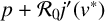$p+\mathcal {R}_{0}j^{\prime }(v^*)$ represents $\mathcal {J}^{\prime }(v^*)$ .

Finally, we conclude that the optimal control $v^*$ for problem (5.6) is characterized by

$$ \begin{align*} \begin{cases} (p+\mathcal{R}_{0}j^{\prime}(v^*),v-v^*)_{0}\geq 0\quad\text{for all } v\in \mathcal{V}_{ad},\\ \mathcal{A}(\xi(v^*))p=\mathcal{R}J^{\prime}(\xi(v^*)),\\ \xi(v^*)- \lambda L_{2}(\xi(v^*))+C(\xi(v^*))-L_{1}(\xi(v^*))=Gv^*+\theta. \end{cases} \end{align*} $$