1. Introduction
Anomalous relativistic [Reference Gzyl17] (see also [Reference Donahue and Dubovsky9]) diffusion processes with finite propagation speed often seem more natural for modelling than the classical diffusion approach. For a detailed discussion, see [Reference Sandev, Kocarev, Metzler and Chechkin32]. There are several different terminological and ideological systems for dealing with such classes of anomalous diffusions. In physics, people prefer to say ‘continuous-time random walks’ [Reference Montroll and Weiss22], ‘flip-flop’ [Reference Brémaud4], or ‘zig-zag processes’ [Reference Donahue and Dubovsky9, Reference Vasdekis and Roberts35]. In mathematics, the terms ‘piecewise-deterministic processes’ [Reference Davis8] or ‘telegraph processes’ [Reference Goldstein14, Reference Kac19, Reference Ratanov and Kolesnik31], are commonly used. The study of classical stochastic differential equations with regime switching (and their applications) is also widely represented; see, for example, [Reference Ratanov25, Reference Yuan and Mao40].
In this paper we study a piecewise deterministic nonlinear system whose dynamics is specified by a double-well potential and a two-state Markov random process. It turns out that such a system can have metastable states as an important feature.
This problem setting continues the author’s previous studies on stochastic differential equations based on piecewise deterministic processes. These studies have recently begun with Ornstein–Uhlenbeck-like processes, where the telegraph process replaces the Wiener process in the Langevin equation. Invariant measures and distributions of first-passage times have been obtained for such stochastic dynamics with its various modifications [Reference Ratanov26, Reference Ratanov27, Reference Ratanov28, Reference Ratanov29, Reference Ratanov30]. Here we develop similar ideas in a nonlinear setting.
Dynamic systems subject to random perturbations are actively studied in both physical and mathematical literature. In the simplest case, such systems are usually based on deterministic dynamics, which follows the ordinary differential equation
 $\textrm{d}\gamma(t)=-U'(\gamma(t))\,\textrm{d} t$
,
 $t>0$
, equipped with a random perturbation, where the function U is the potential.
Let x be a stationary point, i.e.
 $U'(x)=0$
. If
 $U''(x)>0$
, then the position x is asymptotically stable, i.e.
 $\gamma(t)\to x$
as
 $t\to+\infty$
for any starting point near x. On the contrary, if
 $U''(x)<0$
, then x is unstable and repulsive, i.e. any path that starts near x moves away from x. The interplay between different kinds of stationary points under different randomisations of this equation is of special interest. The first and most popular randomisation method is to add a stochastic term, such as white noise, to the deterministic differential equation [Reference Herrmann, Imkeller, Pavlyukevich and Peithmann18]. Later, other randomisation options have emerged, for example the Lévy process [Reference Dybiec and Gudowska-Nowak10], ‘coloured’ noise (e.g. the Ornstein–Uhlenbeck process) [Reference Wilkinson38, Reference Zhang, Liu and He41] and the fractional Gaussian [Reference Goychuk and Kharchenko15].
When the phases coexist, the phenomenon of hysteresis may occur, see the discussion in [Reference Das and Kantz7, Reference Dybiec and Gudowska-Nowak10, Reference Verma, Kumar and Pattanayak37]. An introduction to metastability can be found in [Reference Bovier and den Hollander3].
The simplest case of a one-dimensional setting has recently been generalised in a number of works on metastability effects arising in the case of diffusion processes that are stopped or reflecting on the boundary of a domain [Reference Freidlin and Koralov11] and, more generally, on metastability at and near the surfaces that remain invariant under diffusion processes [Reference Freidlin and Koralov12].
When using various randomisation methods, stochastic resonance can occur, where a small change in the input signal causes a large output signal in the system. Such dynamics, with a transition from one potential well to another, can be interpreted to qualitatively explain glacial cycles in the history of the Earth (from a warm state to an ice age and back) [Reference Herrmann, Imkeller, Pavlyukevich and Peithmann18]. Similar phenomena occur in various applied settings, from biology to metallurgy [Reference Strogatz34]. For example, this approach is effective when modelling a single neuron [Reference Bulsara, Jacobs, Zhou, Moss and Kiss5, Reference Gutkin, Jost and Tuckwell16, Reference Nicolis24, Reference Ratanov26] (see also a recent review of these models in [Reference Carrillo and Roux6]) and artificial neuronal sets [Reference Simonotto, Riani, Seife, Roberts, Twitty and Moss33], as well as dynamics of competing populations [Reference Wissel39] and chemical reaction systems [Reference Vellela and Qian36]. See also detailed overviews of other applications in [Reference Gammaitoni, Hänggi, Jung and Marchesoni13, Reference McDonnell, Stocks, Pearce and Abbott20, Reference Náprstek, Fischer and Awrejcewicz23].
The idea of stochastic resonance is successfully used, for example, by adding white noise
 $\sigma(T)\,\textrm{d} W(t)$
to a deterministic differential equation, where W is standard Brownian motion and the coefficient
 $\sigma(T)$
is chosen to maximise the coefficient of spectral power amplification [Reference Benzi, Parisi, Sutera and Vulpiani1, Reference Nicolis24]. The second approach involves the so-called ‘effective dynamics’, based on a two-state Markov chain with a time-periodic infinitesimal generator, which artificially ensures a spatial interwell transition [Reference Herrmann, Imkeller, Pavlyukevich and Peithmann18].
Our randomisation methodology consists in replacing the diffusion term W(t) by a relativistic (finite-velocity) process
 $\mathbb{T}(t)$
. The idea of such replacement has become more and more popular in physics [Reference Gzyl17, Reference Sandev, Kocarev, Metzler and Chechkin32]. With this randomisation, the model receives certain time windows for interwell transitions instead of stochastic resonance options. In this setting, we present an infinitesimal generator of the process (Theorem 1), compare the probabilities for which attractor the process will end up on when the velocities are small (Theorem 3), and derive formulae for the average first-passage times when the process has already left the metastable position (Theorem 4). Invariant measures inside the attractors are also found (Theorem 6).
The paper is organised as follows. The next section is devoted to the problem setting and a description of the structure of the underlying dynamics. In Section 3 we analyse the distributions of passage times. Section 4 presents invariant distributions.
2. Preliminaries and problem statement
Let
 $\mathbb{T}(t)$
be a telegraph process with alternating velocities
 $c_0, c_1$
,
 $c_0>c_1$
:
 $\mathbb{T}(t)=\int_0^tc_{\xi(s)}\,\textrm{d} s$
,
 $t>0$
, where
 $\xi=\xi(t)\in\{0, 1\}$
is a two-state Markov process with alternating switching intensities
 ${\lambda}_0$
,
 ${\lambda}_1$
[Reference Ratanov and Kolesnik31]. Consider a stochastic process
 $X(t)=X^x(t)$
defined by the equation
 \begin{equation} \textrm d X(t)=-U'(X(t))\,\textrm{d} t+\textrm{d} \mathbb{T}(t),\quad t > 0,\end{equation}
and the initial condition
 $X(0)=x$
. The process
 $X=X(t)$
can be considered as a telegraph process
 $\mathbb{T}$
in the potential U.
Our previous studies [Reference Ratanov26, Reference Ratanov27, Reference Ratanov28, Reference Ratanov29, Reference Ratanov30] were based on the so-called Kac–Ornstein–Uhlenbeck processes, which are defined by the equation
 \begin{equation*}\textrm{d} \bar X(t)=\big(c_{\xi(t)}-\gamma_{\xi(t)}\bar X(t)\big)\,\textrm{d} t,\quad t > 0,\end{equation*}
i.e. the case of alternating single-well potentials
 $U_i=\gamma_ix^2/2-c_ix$
.
For the quasilinear setting (1), suppose that the function U(x),
 $U\in C^2(\!-\!\infty, \infty)$
, is a double-well potential, i.e. it has a local maximum at the point
 $x_0$
, two local minima at the points
 $x_{-},x_+$
,
 $x_{-}<x_0<x_{+}$
, and
 $U''(x)\ne0$
,
 $x\in\{x_-, x_0, x_+\}$
. As a typical example, we can use the symmetric function
 $U(x)=\frac14{x^4}-\frac12{x^2}$
.
The process X(t) is continuous, piecewise continuously differentiable, and is formed by the sequential alternation of two deterministic patterns
 $\gamma_0(t, x)$
and
 $\gamma_1(t, x)$
, which follow the equations
 \begin{equation} \begin{aligned} \frac{{\partial}\gamma_0(t, x)}{{\partial} t}=c_0-U'(\gamma_0(t, x)), \ \frac{{\partial}\gamma_1(t, x)}{{\partial} t}=c_1-U'(\gamma_1(t, x)), \quad t > 0,\ \gamma_0(0, x)=\gamma_1(0, x)=x.\end{aligned} \end{equation}
One pattern is replaced by another at random times
 $\tau_n$
, when the underlying Markov process
 $\xi(t)$
switches.
The initial value problems (2) are equivalent to the pair of integral equations
 \begin{equation} \int_x^{\gamma_0(t, x)}\frac{\textrm{d} z}{c_0-U'(z)}=t,\quad \int_x^{\gamma_1(t, x)}\frac{\textrm{d} z}{c_1-U'(z)}=t, \qquad t \ge 0,\end{equation}
which can be rewritten in the equivalent form
 \begin{equation} \Phi_0(\gamma_0(t, x))=\Phi_0(x)+t, \quad \Phi_1(\gamma_1(t, x))=\Phi_1(x)+t.\end{equation}
Here,
 $\Phi_0$
and
 $\Phi_1$
are rectifying diffeomorphisms defined, up to an arbitrary additive constant, by the equations
 \begin{equation} \Phi_0'(y)=\frac{1}{c_0-U'(y)},\qquad \Phi_1'(y)=\frac{1}{c_1-U'(y)}.\end{equation}
Notice that the function
 $\Phi_i=\Phi_i(y)$
is continuous and monotone between the critical points of the potential
 $U_i=U(x)-c_ix$
.
To avoid blow-up, assume that the integral
 $\int_{x}{\textrm{d} y}/{U_i'(y)}$
diverges at any critical point of
 $U_i$
:
 \begin{equation} \int_{x}\frac{\textrm{d} y}{U_i'(y)}=\infty, \quad x\in\{x_-, x_0, x_+\}.\end{equation}
By definition (3), it follows that the pattern
 $\gamma_i(t, x)$
arising from the state (x, i),
 $i\in\{0, 1\}$
, also satisfies the initial value problem
 \begin{equation} \begin{aligned} \frac{{\partial}\gamma_i}{{\partial} t}(t, x) = L_i^x[\gamma_i(t, x)], \quad t > 0, \ \gamma_i(t, x)\big|_{t\downarrow0} = x,\end{aligned}\end{equation}
where
 $L_i^x=-U_i'(x)({{\partial}}/{{\partial} x})=(c_i-U'(x))({{\partial}}/{{\partial} x})$
,
 $i\in\{0, 1\}$
.
The properties of the process X depend significantly on the velocity amplitudes
 $c_0$
and
 $c_1$
.
A: An unstable uncertainty interval and two attractors
Let both parameters
 $c_0$
and
 $c_1$
be small enough that
 $V>c_0>c_1>v$
, where V and v are, respectively, a local maximum and a local minimum of U
 $^{\prime}$
. In this case, both
 $U_0(x)=U(x)-c_0x$
and
 $U_1(x)=U(x)-c_1x$
are still double-well potentials with alternation between them. Let
 $a_0, a_\pm$
be the critical points of
 $U_1$
,
 $a_-<a_0<a_+$
, and
 $b_0, b_\pm$
be the critical points of
 $U_0$
,
 $b_-<b_0<b_+$
(see Figure 1(a)).
U
 $^{\prime}$
(x) and
 $G_0$
,
 $G_\pm$
.

Note that
 $X(t)\equiv a_-$
,
 $X(t)\equiv a_+$
, and
 $X(t)\equiv a_0$
are stationary solutions of (1) under the initial state
 $\xi(0)=1$
. The pattern
 $\gamma_1=\gamma_1(t, x)$
is repelled by
 $a_0$
, while being attracted to
 $a_-$
or
 $a_+$
. Respectively,
 $X(t)\equiv b_-$
,
 $X(t)\equiv b_+$
, and
 $X(t)\equiv b_0$
are stationary solutions under
 $\xi(0)=0$
, and pattern
 $\gamma_0$
is repelled by
 $b_0$
, being attracted to points
 $b_\pm$
.
As a result, the process X has two attractors,
 $G_-=[a_-, b_-]\subset(\!-\!\infty, b_0)$
and
 $G_+=[a_+, b_+]\subset(a_0, +\infty)$
, and a metastable set
 $G_0=(b_0, a_0)$
. The process
 $X^x$
, starting from the metastable set
 $G_0$
,
 $x\in G_0$
, can temporarily oscillate inside, but once it leaves this interval through the upper or lower bound, it never returns, and then forever remains above
 $a_0$
or below
 $b_0$
, respectively, being attracted to
 $G_+$
or
 $G_-$
. See the sample of a path in Figure 2.
Sample path of X, case A.

If the process
 $X=X^x(t)$
starts from
 $x=X^x(0)>a_0$
, then after a finite transition time it ends up in
 $G_+$
, and when starting from
 $x<b_0$
, the process for almost surely (a.s.) finite time falls into
 $G_-$
.
Note that both sets
 $G_-$
and
 $G_+$
are invariant under dynamics:
 \begin{equation} \begin{aligned} \mathbb{P}\{X(t)\in G_-\ \text{for all}\ t>0 \mid X(0)\in G_-\} & = 1, \\[5pt] \mathbb{P}\{X(t)\in G_+\ \text{for all}\ t>0 \mid X(0)\in G_+\} & = 1. \end{aligned}\end{equation}
Figure 3 shows plots of
 $\Phi_0$
and
 $\Phi_1$
in this case.
Functions
 $\Phi_0(x)$
and
 $\Phi_1(x),$
case A.

B: Alternating single- and double-well potentials, only one attractor
When
 $c_0$
becomes large, so that
 $c_0>V$
, the potential
 $U_0(x)$
has only one critical point
 $b_+$
, becoming single-well, while
 $U_1$
is still double-well, and has three critical points. In this case, the process X has only one attractor
 $G_+$
, see Figure 1(b). After some transition period, with probability 1 X ends up in
 $G_+$
. A symmetric situation occurs when
 $c_1$
becomes less than v, see Fig. 1(c).
C: Alternating single-well potentials, one attractor
In the case
 $c_0>V>v>c_1$
, both potentials
 $U_0$
and
 $U_1$
become single-well. The dynamics has only one attractor
 $G=(a_-, b_+)$
. When the process X begins in
 $x=X(0)\in G$
, it randomly fluctuates between the attractive levels
 $a_-$
and
 $b_+$
. If it starts outside, then it ends at G after some transition.
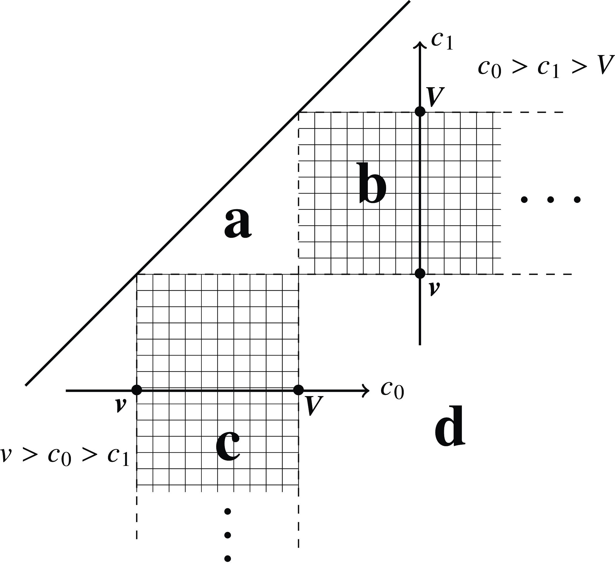
Two other less interesting single-well situations with a single attractor are not shown in Figure 1. They correspond to
 $c_0>c_1>V>v$
and
 $c_1<c_0<v<V$
. See Figure 4 for a diagram of the different regimes.
Scheme of different modes. Triangle
 $\textbf{a}$
,
 $V>c_0>c_1>v$
(case A); half-bands
 $\textbf{b}$
and
 $\textbf{c}$
, corresponding to
 $c_0>V>c_1>v$
and
 $V>c_0>v>c_1$
respectively (case B); quadrant
 $\textbf{d}$
,
 $c_0>V>v>c_1$
(case C). (Designations according to Figure 1.)

The process
 $\Xi=(X^x(t),\,\xi(t))$
is a Markov process with the state space
 $\mathbb{R}\times\{0,1\}$
. Let
 $\tau^0$
be the time of first switching from state 0 to state 1;
 $\tau^1$
corresponds to the reverse switching. Due to the Markov property, the following equalities in distribution hold:
 \begin{equation} \begin{aligned}{} [X^x(t) \mid \xi(0)=0] & \stackrel{\textrm{D}}{=} \gamma_0(t, x)\cdot{1}_{\{\tau^{0} > t\}} + {1}_{\{\tau^{0} < t\}} \cdot \big[X^{\gamma_0(\tau^{0}, x)}(t-\tau^{0}) \mid \xi(0)=1\big], \\[5pt] [X^x(t) \mid \xi(0)=1] & \stackrel{\textrm{D}}{=} \gamma_1(t, x)\cdot{1}_{\{\tau^1 > t\}} + {1}_{\{\tau^1 < t\}}\cdot\big[X^{\gamma_1(\tau^1, x)}(t-\tau^1) \mid \xi(0)=0\big]. \end{aligned}\end{equation}
Based on (9), we can obtain an infinitesimal generator of
 $\Xi$
.
Theorem 1. The infinitesimal generator of
 $\Xi$
is given by
 $\Lambda+\mathcal{L}$
, where
 $$ \Lambda = \begin{pmatrix} -{\lambda}_0\;\;\;\; & {\lambda}_0 \\[5pt] {\lambda}_1\;\;\;\; & -{\lambda}_1 \end{pmatrix} $$
is the generator of the two-state Markov process
 $\xi$
, and
 \begin{equation} \mathcal{L}=\mathcal{L}^x = \begin{pmatrix} L_0^x\;\;\;\; & 0 \\[5pt] 0\;\;\;\; & L_1^x \end{pmatrix}. \end{equation}
See the proof in the Appendix.
3. Passage times
Let
 $\mathcal{T}(x, y)$
be the time when the process X(t) first reaches a given threshold y, starting from point x:
 $\mathcal{T}(x, y)=\inf\{t > 0 \mid X(0)=x,\,X(t)=y\}$
. The distribution of this random variable is determined by the moment-generating function
 $\boldsymbol{u}=(u_0(q, x, y),\,u_1(q, x, y))^\top$
,
 \begin{equation*} \begin{aligned} u_0(q, x, y)&=\mathbb{E}[\!\exp(\!-\!q\mathcal{T}(x, y)) \mid \xi(0)=0], \\[5pt] u_1(q, x, y)&=\mathbb{E}[\!\exp(\!-\!q\mathcal{T}(x, y)) \mid \xi(0)=1], \end{aligned} \quad q > 0.\end{equation*}
We denote By
 $t_0^*(x, y)$
and
 $t_1^*(x, y)$
the time to reach level y without switching states, starting from (x, 0) and (x, 1), respectively. The value
 $t_i^*(x, y)$
is finite if the equation
 $\gamma_i(t, x)=y$
is satisfied for some positive t,
 $t=t_i^*(x, y)$
. In this case we say that level y is reachable from state (x, i). Otherwise we set
 $t_i^*(x, y)=\infty$
.
If y is reachable from the state (x, i), then both x and y belong to the domain of a common continuous piece of
 $\Phi_i$
; moreover, since (4) holds,
 $\Phi_i(y)>\Phi_i(x)$
and
 $t_i^*(x, y)=\Phi_i(y)-\Phi_i(x)$
. Also,
 $\lim_{x\to y}t_i^*(x, y)=0$
.
By virtue of (5),
 \begin{equation} L_i^xt_i^*(x, y)=-L_i^x\Phi_i(x)=-1 \quad \text{when $t_i^*(x, y)$ is finite},\ i\in\{0, 1\}.\end{equation}
Let y be a level reachable from both (x, 0) and (x, 1). Conditioning on the first switching, like in (9), we obtain a system of integral equations:
 \begin{equation} \left\{ \begin{aligned} u_0(q, x, y) & = \textrm{e}^{-(q+{\lambda}_0)t_0^*(x, y)} + \int_0^{t_0^*(x, y)}{\lambda}_0\textrm{e}^{-(q+{\lambda}_0)\tau}u_1(q,\gamma_0(\tau,x),y)\,\textrm{d}\tau, \\[5pt] u_1(q, x, y) & = \textrm{e}^{-(q+{\lambda}_1)t_1^*(x, y)} + \int_0^{t_1^*(x, y)}{\lambda}_1\textrm{e}^{-(q+{\lambda}_1)\tau}u_0(q,\gamma_1(\tau,x),y)\,\textrm{d}\tau. \end{aligned} \right.\end{equation}
On the contrary, in the case
 $t_i^*(x, y)=+\infty$
, the corresponding integral equation of (12) can be interpreted as
 \begin{equation} u_i(q, x, y) = \int_0^\infty{\lambda}_i\textrm{e}^{-(q+{\lambda}_i)\tau}u_{1-i}(q,\gamma_i(\tau,x),y)\,\textrm{d}\tau, \quad i\in \{0, 1\}.\end{equation}
Theorem 2. The moment-generating function
 $\boldsymbol{u}=(u_0(q, x, y),\,u_1(q, x, y))^\top$
of the first-passage time
 $\mathcal{T}(x, y)$
satisfies
 \begin{equation} \big(\Lambda+\mathcal{L})\boldsymbol{u}(q, x, y)=q\boldsymbol{u}(q, x, y),\quad q>0, \end{equation}
where
 $\Lambda+\mathcal{L}$
is the generator of the Markov process
 $\Xi$
.
Both entries
 $u_0(q, x, y)$
and
 $u_1(q, x, y)$
of
 $\boldsymbol{u}$
separately obey telegraph [Reference Borodin and Gorin2] equations of the form
 \begin{equation} \begin{aligned} L_1^xL_0^xu_0(q, x, y)-\big[(q+{\lambda}_1)L_0^x+(q+{\lambda}_0)L_1^x\big]u_0(q, x, y) +q(q+{\lambda}_0+{\lambda}_1)u_0(q, x, y)&=0,\\[5pt] L_0^xL_1^xu_1(q, x, y)-\big[(q+{\lambda}_1)L_0^x+(q+{\lambda}_0)L_1^x\big]u_1(q, x, y) +q(q+{\lambda}_0+{\lambda}_1)u_1(q, x, y)&=0. \end{aligned} \end{equation}
Equations (14) and (15) are provided with boundary conditions that depend on whether the level y is reachable from (x, 0) and (x, 1).
Proof. Apply
 $L_0^x$
and
 $L_1^x$
to the first and second equations of the system (12), respectively.
First, let the threshold y be reachable from (x, 0). By virtue of (7) and (11), the first equation of (12) yields
 \begin{align*} \begin{aligned} L_0^xu_0(q, x, y) & = (q+{\lambda}_0)\textrm{e}^{-(q+{\lambda}_0)t_0^*(x, y)} - {\lambda}_0\textrm{e}^{-(q+{\lambda}_0)t_0^*(x, y)}u_1(q, \gamma_0(t_0^*(x, y), x), y) \\[5pt] & \quad + \int_0^{t_0^*(x, y)}{\lambda}_0\textrm{e}^{-(q+{\lambda}_0)\tau} \frac{{\partial}}{{\partial}\tau}[u_1(q, \gamma_0(\tau, x), y)]\,\textrm{d}\tau. \end{aligned} \end{align*}
Integrating by parts, we can see that
 \begin{align*} \begin{aligned} L_0^xu_0(q, x, y) & = (q+{\lambda}_0)\textrm{e}^{-(q+{\lambda}_0)t_0^*(x, y)} - {\lambda}_0u_1(q, x, y) \\[5pt] & \quad + (q+{\lambda}_0)\int_0^{t_0^*(x, y)}{\lambda}_0\textrm{e}^{-(q+{\lambda}_0)\tau}u_1(q,\gamma_0(\tau,x),y)\, \textrm{d}\tau. \end{aligned} \end{align*}
Proceeding similarly with the second equation of (12), both in the case of finite and infinite
 $t_1^*(x, y)$
, we obtain the system
 \begin{equation} \left\{ \begin{aligned} L_0^xu_0(q, x, y) & = (q+{\lambda}_0)u_0(q, x, y)-{\lambda}_0u_1(q, x, y), \\[5pt] L_1^xu_1(q, x, y) & = -{\lambda}_1u_0(q, x, y)+(q+{\lambda}_1)u_1(q, x, y), \end{aligned} \right.\end{equation}
which in matrix form coincides with (14).
Equations (15) follow from (16) by eliminating variables. Indeed, applying
 $L_1^x$
to the first equation of system (16), we get
 $L_1^xL_0^xu_0(q, x, y)=(q+{\lambda}_0)L_1^xu_0(q, x, y)-{\lambda}_0L_1^xu_1(q, x, y)$
. From the second equation of (16) we obtain
 \[ L_1^xL_0^xu_0(q, x, y) = (q+{\lambda}_0)L_1^xu_0(q, x, y) + {\lambda}_0{\lambda}_1u_0(q, x, y) - {\lambda}_0(q+{\lambda}_1)u_1(q, x, y).\]
The first equation of (16) can be rewritten as
 ${\lambda}_0u_1(q, x, y)=(q+{\lambda}_0)u_0(q, x, y)-L_0^xu_0(q, x, y)$
, which gives the first equation of (15); the second equation is obtained similarly.
If
 $\mathbb{P}\{\mathcal{T}(x, y) < \infty\}=1$
, then the mean value
 $\boldsymbol{m}(x, y)=(m_0(x, y),\, m_1(x, y))^\top$
,
 \[ m_0(x, y)=\mathbb{E}[\mathcal{T}(x,y) \mid \xi(0)=0], \quad m_1(x, y)=\mathbb{E}[\mathcal{T}(x,y) \mid \xi(0)=1],\]
can be found by differentiation:
 \begin{equation*} m_0(x, y) = -\frac{{\partial} u_0(q, x, y)}{{\partial} q}\bigg|_{q=0}, \quad m_1(x, y) = -\frac{{\partial} u_1(q, x, y)}{{\partial} q}\bigg|_{q=0}.\end{equation*}
Theorem 2 implies the following result, general for Markov processes.
Corollary 1. Let the mean value of
 $\mathcal{T}(x, y)$
be finite. Then the mean vector
 $\boldsymbol{m}(x, y)$
satisfies the equation
 \begin{equation} (\Lambda+\mathcal{L}^x)\boldsymbol{m}(x, y)=-\textbf{1}=(1, 1)^\top. \end{equation}
Let us first consider the case of small
 $c_0$
and
 $c_1$
, i.e.
 $V>c_0>c_1>v$
, see Figure 1(a).
3.1. Small
 $\boldsymbol{c}_{\textbf{0}}$
and
$\boldsymbol{c}_{\textbf{1}}$
: Probabilities of leaving the uncertainty interval


In the case
 $V>c_0>c_1>v$
, let the initial point x be inside the interval
 $G_0$
, i.e.
 $X(0)=x\in G_0=(b_0, a_0)$
– case A, Figure 1(a).
Since both
 $a_0$
and
 $b_0$
are repulsive, a trajectory that has crossed one of these thresholds once never returns to the interval
 $(b_0, a_0)$
. We are interested in the conditional probabilities of exiting the interval
 $G_0=(b_0, a_0)$
through the upper bound
 $a_0$
,
 \begin{equation} p_0(x)=\mathbb{P}\{\mathcal{T}(x, a_0) < \infty \mid \xi(0)=0\}, \quad p_1(x)=\mathbb{P}\{\mathcal{T}(x, a_0) < \infty \mid \xi(0)=1\}.\end{equation}
The moment-generating functions
 $u_0(q, x, a_0)$
and
 $u_1(q, x, a_0)$
,
 $x\in G_0$
, are increasing. Further,
 $0 < u_0(q, x, a_0) < 1$
and
 $0 < u_1(q, x, a_0) < 1$
for
 $b_0<x<a_0$
. Moreover,
 \begin{align*} \begin{aligned} \lim_{q\downarrow0}[u_0(q, x, a_0)] & = \mathbb{P}\{\mathcal{T}(x,a_0) < \infty \mid {\varepsilon}(0)=0\} = p_0(x), \\[5pt] \lim_{q\downarrow0}[u_1(q, x, a_0)] & = \mathbb{P}\{\mathcal{T}(x, a_0) < \infty \mid {\varepsilon}(0)=1\} = p_1(x) \end{aligned}\end{align*}
are the probabilities of leaving the interval
 $(b_0, a_0)$
through the upper bound
 $a_0$
, starting from the position
 $X(0)=x$
with the initial state
 $\xi(0)=0$
and
 $\xi(0)=1$
, respectively.
The probabilities
 $p_0(x)$
and
 $p_1(x)$
depend on the constants
 \begin{equation} B_0=\int_{b_0}^{a_0}\frac{\Psi(y)}{c_0-U'(y)}\,\textrm{d} y, \qquad B_1=\int_{b_0}^{a_0}\frac{\Psi(y)}{c_1-U'(y)}\,\textrm{d} y.\end{equation}
Here,
 $\Psi(y)=\exp\left({\lambda}_0\Phi_0(y)+{\lambda}_1\Phi_1(y)\right)$
.
The integrals in (19) converge, since
 \[ \bigg|\frac{\Psi(y)}{c_i-U'(y)}\bigg| \le \textrm{const}\cdot\exp({\lambda}_i\Phi_i(y)) \cdot |\Phi_i'(y)|, \quad y\in G_0,\]
and
 \[ \int_{b_0}^{a_0}\textrm{e}^{{\lambda}_i\Phi_i(y)}|\Phi_i'(y)|\,\textrm{d} y = \Big|\exp({\lambda}_i\Phi_i(y))\big|_{y=b_0+}^{y=a_0-}\Big| < \infty.\]
See Figure 3.
Theorem 3. Let
 $X(0)=x$
,
 $x\in(b_0,\;a_0)$
. The probabilities
 $p_0(x)$
and
 $p_1(x)$
defined by (18) have the form
 \begin{align} p_0(x) & = \mathbb{P}\{\mathcal{T}(x, a_0) < \infty \mid \xi(0)=0\} = 1 - B_0^{-1}\int_x^{a_0}\frac{\exp({\lambda}_0\Phi_0(y)+{\lambda}_1\Phi_1(y))}{c_0-U'(y)}\,\textrm{d}y, \end{align}
 \begin{align} p_1(x) & = \mathbb{P}\{\mathcal{T}(x, a_0) < \infty \mid \xi(0)=1\} = B_1^{-1}\int_{b_0}^x\frac{\exp({\lambda}_0\Phi_0(y)+{\lambda}_1\Phi_1(y))}{c_1-U'(y)}\,\textrm{d}y, \end{align}
where
 $B_0, B_1$
are defined by (19).
Proof. By definition, it follows that
 \begin{equation} p_0(x)\big|_{x\uparrow a_0}=1, \quad p_1(x)\big|_{x\downarrow b_0}=0, \quad q>0.\end{equation}
Conditioning on the first switching, like in (9), similarly to (12), we obtain
 \begin{equation} u_0(0, x, a_0)=p_0(x)=\textrm{e}^{-{\lambda}_0t_0^*(x, a_0)} +\int_0^{t_0^*(x, a_0)}{\lambda}_0\textrm{e}^{-{\lambda}_0\tau}p_1(\gamma_0(\tau, x))\,\textrm{d}\tau.\end{equation}
Since the process X leaving the interval
 $G_0$
through the lower bound forever remains below
 $b_0$
, instead of (23) and (13) we obtain
 \begin{equation} u_1(0, x, a_0)=p_1(x)=\int_0^{t_1^*(x, b_0)}{\lambda}_1\textrm{e}^{-{\lambda}_1\tau} p_0(\gamma_1(\tau, x))\,\textrm{d}\tau.\end{equation}
Here,
 $t_0^*(x, a_0)=\Phi_0(a_0)-\Phi_0(x)$
and
 $t_1^*(x, b_0)=\Phi_1(b_0)-\Phi_1(x)$
; function
 $\Phi_0$
is increasing, and function
 $\Phi_1$
is decreasing on
 $(b_0, a_0)$
.
From (23) and (24), in the usual way by applying
 $L_0^x$
and
 $L_1^x$
followed by integration by parts, differential equations similar to (15) and (16) are derived: first
 $(\Lambda+\mathcal{L})\textbf{p}(x)=\textbf{0}$
and
 $\textbf{p}(x)=(p_0(x), p_1(x))^\top$
, and then
 \begin{equation} \begin{aligned} L_1^xL_0^x p_0(x) - ({\lambda}_1L_0^x+{\lambda}_0L_1^x)p_0(x) & = 0, \\[5pt] L_0^xL_1^x p_1(x) - ({\lambda}_1L_0^x+{\lambda}_0L_1^x)p_1(x) & = 0. \end{aligned}\end{equation}
See Theorem 2.
Let
 \begin{equation} v_0(x)=L_0^x[p_0](x),\qquad v_1(x)=L_1^x[p_1](x).\end{equation}
Note that the functions
 $p_0(x)$
and
 $p_1(x)$
increase,
 $x\in G_0$
.
Since
 $c_1<U'(x)<c_0$
,
 $v_0(x)>0$
and
 $v_1(x)<0$
for all
 $x\in G_0$
. Using this notation, equations (25) take the form
 \begin{align*} \begin{aligned} (c_1-U'(x))\frac{{\partial} v_0}{{\partial} x}(x) - {\lambda}_1v_0(x) - {\lambda}_0\frac{c_1-U'(x)}{c_0-U'(x)}v_0(x) & = 0, \\[5pt] (c_0-U'(x))\frac{{\partial} v_1}{{\partial} x}(x) - {\lambda}_1\frac{c_0-U'(x)}{c_1-U'(x)}v_1(x) - {\lambda}_0v_1(x) & = 0, \end{aligned} \end{align*}
which can be rewritten as
 \begin{equation} \begin{aligned} \frac{\textrm{d} v_0}{\textrm{d} x}(x)=\psi(x)v_0(x), \qquad \frac{\textrm{d} v_1}{\textrm{d} x}(x)=\psi(x)v_1(x), \qquad b_0 < x < a_0, \end{aligned} \end{equation}
where
 \begin{equation} \psi(x) = \frac{{\lambda}_0}{c_0-U'(x)}+\frac{{\lambda}_1}{c_1-U'(x)}.\end{equation}
From (27) and (28), by definition (5) we obtain
 \begin{equation*} v_0(x)=A_0\exp({\lambda}_0\Phi_0(x)+{\lambda}_1\Phi_1(x)), \qquad v_1(x)=A_1\exp({\lambda}_0\Phi_0(x)+{\lambda}_1\Phi_1(x))\end{equation*}
with indefinite constants
 $A_0$
and
 $A_1$
.
Taking into account boundary conditions (22), we obtain
 \[ p_0(x)=-\int_x^{a_0}\frac{v_0(y)}{c_0-U'(y)}\,\textrm{d} y+1, \qquad p_1(x)=\int_{b_0}^x \frac{v_1(y)}{c_1-U'(y)}\,\textrm{d} y.\]
By the no-blow-up condition (6), we can see that
 $A_0=B_0^{-1}$
and
 $A_1=B_1^{-1}$
, which gives the solution to equations (26) in the form (20) and (21).
3.2. Starting near the attractor
Let the initial point x and the threshold y be located near (or inside) the attractor. We study only the case of the upper half-line,
 $x, y>a_0$
, and the attractor
 $G_+$
, see Figure 1(a) and (b). This is sufficient because the case of
 $x, y<b_0$
and the attractor
 $G_-$
, Figure 1(a) and (c), is symmetric.
Since both levels
 $a_+$
and
 $b_+$
are attractive, and
 $a_0, b_0$
are repulsive, the process
 $X=X(t)$
increases a.s. moving along the set
 $(a_0,a_+)$
and decreases moving along the set
 $[b_+,+\infty)$
. Therefore,
 $\mathcal{T}(x,y)\big|_{x > y \ge a_0} = \infty$
,
 $\mathcal{T}(x,y)\big|_{b_+\le x < y}=\infty$
a.s. Inside the attractor
 $G_+$
, the process
 $X=X(t)$
randomly oscillates between the attractive levels
 $a_+$
and
 $b_+$
.
The mean value
 $\boldsymbol{m}(x, y)=(m_0(x, y),\, m_1(x, y))^\top$
can be expressed through the integrals
 \begin{align} I_0(x,y) & = \int_x^y\frac{\beta(z_0, y)\,\textrm{d} z_0}{c_0-U'(z_0)}, \qquad I_1(x,y) = \int_x^y\frac{\beta(z_1, y)\,\textrm{d} z_1}{c_1-U'(z_1)}, \end{align}
 \begin{align} J_0(x,y) & = \int_{\Delta_0(x, y)}\frac{\beta(z_0, z_1)}{(c_0-U'(z_0))(c_1-U'(z_1))}\,\textrm{d}z_0\,\textrm{d}z_1, \end{align}
 \begin{align} J_1(x,y) & = \int_{\Delta_1(x, y)}\frac{\beta(z_1, z_0)}{(c_0-U'(z_0))(c_1-U'(z_1))}\,\textrm{d}z_0\,\textrm{d}z_1. \end{align}
Here,
 $\beta(x, y)={\Psi(x)}/{\Psi(y)}=\exp({\lambda}_0(\Phi_0(x)-\Phi_0(y))+{\lambda}_1(\Phi_1(x)-\Phi_1(y)))$
, and
 $\Delta_0(x, y), \Delta_1(x, y)\subset\mathbb{R}^2$
are two triangles defined by
 \begin{align*} \begin{aligned} \Delta_0(x, y) & = \{(z_0, z_1) \mid x < z_0 < y,\,z_0 < z_1 < y\}, \\[5pt] \Delta_1(x, y) & = \{(z_0, z_1) \mid x < z_1 < y, \, z_1 < z_0 < y\}. \end{aligned} \end{align*}
According to the above definitions, in both cases
 $a_0 < x < y \le a_+$
(with U
 $^{\prime}$
(x),
 $U'(y)<c_1<c_0$
) and
 $x>y\ge b_+$
(with U
 $^{\prime}$
(x),
 $U'(y)>c_0>c_1$
), the integrals
 $I_0(x, y),I_1(x, y)$
and
 $J_0(x, y), J_1(x, y)$
converge.
Theorem 4.
-
(i) Let
$x, y > a_0$
, see Figure 1(a) and (b). The mean values
$m_0(x, y)$
and
$m_1(x, y)$
are given explicitly as follows.-
• In both cases
$x<y<a_+$
and
$x>y>b_+$
, (32)
\begin{align} m_0(x, y) & = I_0(x, y)+({\lambda}_0+{\lambda}_1)J_0(x, y), \end{align}
(33)
\begin{align} m_1(x, y) & = I_1(x, y)+({\lambda}_0+{\lambda}_1)J_1(x, y). \end{align}
-
• If
$x<y$
and
$y\in[a_+, b_+)$
, (34)
\begin{align} m_0(x, y) & = (1+{\lambda}_0/{\lambda}_1)I_0(x, y)+({\lambda}_0+{\lambda}_1)J_0(x, y), \\[-8pt] & \nonumber \end{align}
(35)
\begin{align} m_1(x, y) & = {1}/{{\lambda}_1}+({\lambda}_0+{\lambda}_1)J_1(x, y). \end{align}
-
• If
$x>y$
and
$y\in(a_+, b_+]$
, (36)
\begin{align} m_0(x, y) & = {1}/{{\lambda}_0}+({\lambda}_0+{\lambda}_1)J_0(x, b_+), \\[-8pt] & \nonumber \end{align}
(37)
\begin{align} m_1(x, y) & = (1+{\lambda}_0/{\lambda}_1)I_1(x, b_+)+({\lambda}_0+{\lambda}_1)J_1(x, b_+). \end{align}
-
-
(ii) Let
$x, y<b_0$
, see Figure 1(a) and (c). The mean values
$m_0(x, y)$
and
$m_1(x, y)$
are determined by the following formulae, symmetrical to those given above.-
• In both cases
$x>y>b_-$
and
$x<y<a_-$
, (38)
\begin{align} m_0(x, y) & = I_0(x, y)+({\lambda}_0+{\lambda}_1)J_0(x, y), \end{align}
(39)
\begin{align} m_1(x, y) & = I_1(x, y)+({\lambda}_0+{\lambda}_1)J_1(x, y). \end{align}
-
• If
$x>y$
and
$y\in[a_-,b_-)$
, (40)
\begin{align} m_0(x, y) & = {1}/{{\lambda}_0}+({\lambda}_0+{\lambda}_1)J_0(x, y), \\[-8pt] & \nonumber \end{align}
(41)
\begin{align} m_1(x, y) & = (1+{\lambda}_1/{\lambda}_0)I_1(x, y)+({\lambda}_0+{\lambda}_1)J_1(x, y). \end{align}
-
• If
$x<y$
and
$y\in(a_-,b_-]$
, (42)
\begin{align} m_0(x, y) & = (1+{\lambda}_1/{\lambda}_0)I_0(x, b_+)+({\lambda}_0+{\lambda}_1)J_0(x, b_+), \\[-8pt] \nonumber \end{align}
(43)
\begin{align} m_1(x, y) & = {1}/{{\lambda}_1}+({\lambda}_0+{\lambda}_1)J_1(x, b_+). \end{align}
-


Notice that X is structured in such a way that if this process begins with
 $x\in(a_0,a_+]$
or with
 $x\in[b_+,+\infty)$
, (symmetrically,
 $x\in[b_-, b_0)$
or
 $x\in(\!-\!\infty, a_-]$
) then with probability 1 it ends up inside the set
 $G_+$
(
 $G_-$
) and remains there forever, randomly fluctuating between two attracting thresholds
 $a_+$
and
 $b_+$
.
In the rest of the paper, all proofs for the lower half-line (
 $x<b_0$
) are symmetric to the proofs for
 $x>a_0$
, so we present only the latter.
To prove Theorem 4, we need an auxiliary result that is important in itself.
Lemma 1. Under the conditions of Theorem 4, the mean value of
 $\mathcal{T}(x, y)$
is finite and the entries
 $m_0(x, y)$
and
 $m_1(x, y)$
of the mean vector
 $\boldsymbol{m}(x, y)$
are positive solutions of (17). Furthermore:
-
• If
$a_0<x<y<a_+$
$(b_0>x>y>b_-)$
or
$x>y>b_+$
$(x<y<a_-)$
, then (17) is supplied with the zero boundary condition
$\boldsymbol{m}(x, y)|_{x\to y}=\textbf{0}$
. -
• If
$x<y$
and
$y\in[a_+, b_+)$
, (44)if
\begin{equation} m_0(x, y)|_{x\to y}=0,\qquad m_1(x, y)|_{x\to y}=1/{\lambda}_1; \end{equation}
$x>y$
and
$y\in(a_-, b_-]$
, (45)
\begin{equation} m_0(x, y)|_{x\to y}=1/{\lambda}_0,\qquad m_1(x, y)|_{x\to y}=0. \end{equation}
-
• If
$x>y$
and
$y\in(a_+, b_+]$
, (46)if
\begin{equation} m_0(x, y)|_{x\to y}=1/{\lambda}_0,\qquad m_1(x, y)|_{x\to y}=0; \end{equation}
$x<y$
and
$y\in[a_-, b_-)$
, (47)
\begin{equation} m_0(x, y)|_{x\to y}=0,\qquad m_1(x, y)|_{x\to y}=1/{\lambda}_1. \end{equation}






Moreover,
 $m_0(x, y)$
and
 $m_1(x, y)$
satisfy separate second-order equations:
 \begin{equation} \left\{ \begin{aligned} L_1^xL_0^xm_0(x, y) - \big({\lambda}_1L_0^x+{\lambda}_0L_1^x\big)m_0(x, y) & = {\lambda}_0+{\lambda}_1, \\[5pt] L_0^xL_1^xm_1(x, y) - \big({\lambda}_1L_0^x+{\lambda}_0L_1^x\big)m_1(x, y) & = {\lambda}_0+{\lambda}_1. \end{aligned} \right. \end{equation}
Proof. First, note that if
 $a_0<x<y<a_+$
or
 $x>y>b_+$
, then
 $t_0^*(x, y)$
and
 $t_1^*(x, y)$
are both finite,
 $t_0^*(x, y)|_{x\to y}=t_1^*(x, y)|_{x\to y}=0$
, functions
 $u_0$
and
 $u_1$
follow the coupled integral equations (12),
 $\mathcal{T}(x, y) < \infty$
a.s., and
 $u_0(0, x, y)=u_1(0, x, y)=1$
. Differentiating in (12) with respect to q and then setting
 $q=0$
, we obtain the integral equations
 \begin{equation} \left\{ \begin{aligned} m_0(x, y) & = t_0^*(x, y)\textrm{e}^{-{\lambda}_0t_0^*(x, y)} + \int_0^{t_0^*(x, y)}{\lambda}_0\tau\textrm{e}^{-{\lambda}_0\tau}\,\textrm{d}\tau + \int_0^{t_0^*(x, y)}{\lambda}_0\textrm{e}^{-{\lambda}_0\tau}m_1(\gamma_0(\tau, x), y)\,\textrm{d}\tau, \\[5pt] m_1(x, y) & = t_1^*(x, y)\textrm{e}^{-{\lambda}_1t_1^*(x, y)} + \int_0^{t_1^*(x, y)}{\lambda}_1\tau\textrm{e}^{-{\lambda}_1\tau}\,\textrm{d}\tau + \int_0^{t_1^*(x, y)}{\lambda}_1\textrm{e}^{-{\lambda}_1\tau}m_0(\gamma_1(\tau, x), y)\,\textrm{d}\tau. \end{aligned} \right.\end{equation}
After simplification, the system (49) becomes
 \begin{equation} \left\{ \begin{aligned} m_0(x, y) & = \frac{1-\textrm{e}^{-{\lambda}_0t_0^*(x, y)}}{{\lambda}_0} + \int_0^{t_0^*(x, y)}{\lambda}_0\textrm{e}^{-{\lambda}_0\tau}m_1(\gamma_0(\tau, x), y)\,\textrm{d}\tau, \\[5pt] m_1(x, y) & = \frac{1-\textrm{e}^{-{\lambda}_1t_1^*(x, y)}}{{\lambda}_1} + \int_0^{t_1^*(x, y)}{\lambda}_1\textrm{e}^{-{\lambda}_1\tau}m_0(\gamma_1(\tau, x), y)\,\textrm{d}\tau. \end{aligned} \right.\end{equation}
Note that in cases A and B, the interval
 $G_+$
attracts both patterns,
 $\gamma_0(t, x)$
and
 $\gamma_1(t, x)$
. Therefore,
 $t_i^*(x, y)|_{x\to y}=0$
if
 $x<y<a_+$
or
 $x>y>b_+$
. By (50), this yields the zero boundary condition for (17):
 $m_i(x, y)|_{x\to y}=0$
,
 $i\in\{0, 1\}$
.
If
 $x<y=a_+$
, then
 $t_0^*(x,y)$
is still finite,
 $t_0^*(x, y)|_{x\uparrow y}=0$
, and
 $t_1^*(x, y)=\infty$
. In this case, the first equations in (49) and (50) remain the same. Hence,
 $m_0(x, y)|_{x\uparrow y}=0$
. The second equation in (50) takes the form
 \begin{equation*} m_1(x, y) = \frac{1}{{\lambda}_1} + \int_0^\infty{\lambda}_1\textrm{e}^{-{\lambda}_1\tau}m_0(\gamma_1(\tau, x), y)\,\textrm{d}\tau,\end{equation*}
which gives the same differential equation as before and the boundary condition (44).
If
 $x>y=b_+$
, then similar reasoning again leads to the boundary condition (46).
By eliminating variables (as in Theorem 2), we can see that
 $m_0(x, y)$
and
 $m_1(x, y)$
satisfy the two separate second-order equations (48).
Proof of Theorem 4. This is similar to the proof of Theorem 3. It consists of two steps. First, we transform the system (48) of second-order equations into a system of first-order equations for the functions
 \begin{equation} v_0(x, y)\;:\!=\;L_0^xm_0(x, y),\qquad v_1(x, y)\;:\!=\;L_1^xm_1(x, y). \end{equation}
Note that (51) can be solved in the form
 \begin{equation} \begin{aligned} m_0(x, y)&=\left.m_0(x, y)\right|_{x=y}-\int_x^y\frac{v_0(z_0, y)}{c_0-U'(z_0)}\,\textrm{d} z_0, \\[5pt] m_1(x, y)&=\left.m_1(x, y)\right|_{x=y}-\int_x^y\frac{v_1(z_1, y)}{c_1-U'(z_1)}\,\textrm{d} z_1. \end{aligned} \end{equation}
Second, the formulae in (52) will give the answer if we find
 $v_0$
and
 $v_1$
.
For the first step, by the definition of
 $L_0^x$
and
 $L_1^x$
,
 \[ L_0^xm_1(x, y)=\frac{c_0-U'(x)}{c_1-U'(x)}\cdot v_1(x, y),\qquad L_1^xm_0(x, y)=\frac{c_1-U'(x)}{c_0-U'(x)}\cdot v_0(x, y). \]
Applying the change of variables (51) to (48), we get
 \begin{align*} \begin{aligned} (c_1-U'(x))\frac{{\partial} v_0(x, y)}{{\partial} x} - {\lambda}_1v_0(x, y) - {\lambda}_0\frac{c_1-U'(x)}{c_0-U'(x)}v_0(x, y) & = {\lambda}_0+{\lambda}_1, \\[5pt] (c_0-U'(x))\frac{{\partial} v_1(x, y)}{{\partial} x} - {\lambda}_1\frac{c_0-U'(x)}{c_1-U'(x)}v_1(x, y) - {\lambda}_0v_1(x, y) & = {\lambda}_0+{\lambda}_1. \end{aligned} \end{align*}
Thus, system (48) is equivalent to
 \begin{equation} \left\{ \begin{aligned} \frac{{\partial} v_0}{{\partial} x}(x, y) & = \psi(x)v_0(x, y)+\frac{{\lambda}_0+{\lambda}_1}{c_1-U'(x)}, \\[5pt] \frac{{\partial} v_1}{{\partial} x}(x, y) & = \psi(x)v_1(x, y)+\frac{{\lambda}_0+{\lambda}_1}{c_0-U'(x)}, \end{aligned} \right. \end{equation}
where
 $\psi(x)$
is defined by (28):
 $$\psi(x)=\dfrac{{\lambda}_0}{c_0-U'(x)}+\dfrac{{\lambda}_1}{c_1-U'(x)}=\frac{\Psi'(x)}{\Psi(x)}.$$
The solution of (53) is determined by the boundary conditions that follow from Lemma 1.
For the second step, consider the case
 $a_0<x<y<a_+$
with
 $U'(x),U'(y)<c_1<c_0$
. The case
 $x>y>b_+$
is symmetric with
 $U'(x),U'(y)>c_0>c_1$
.
Since, in this case,
 $\boldsymbol{m}(x, y)|_{x\to y}=\textbf{0}$
(Lemma 1), by virtue of (17), the system (53) is supplied with the boundary conditions
 $v_0(x, y)|_{x\uparrow y}=v_1(x, y)|_{x\uparrow y}=-1$
. Therefore,
 \begin{align} v_0(z_0, y) & = \Psi(z_0)\Psi(y)^{-1}\bigg[{-}1 - ({\lambda}_0+{\lambda}_1)\int_{z_0}^y\frac{\Psi(y)\Psi(z_1)^{-1}}{c_1-U'(z_1)}\,\textrm{d}z_1\bigg] \nonumber \\[5pt] & = -\beta(z_0, y) - ({\lambda}_0+{\lambda}_1)\int_{z_0}^y\frac{\beta(z_0, z_1)}{c_1-U'(z_1)}\,\textrm{d}z_1, \end{align}
 \begin{align} v_1(z_1, y) & = \Psi(z_1)\Psi(y)^{-1}\bigg[{-}1 - ({\lambda}_0+{\lambda}_1)\int_{z_1}^y\frac{\Psi(y)\Psi(z_0)^{-1}}{c_0-U'(z_0)}\,\textrm{d}z_0\bigg] \nonumber \\[5pt] & = -\beta(z_1, y) - ({\lambda}_0+{\lambda}_1)\int_{z_1}^y\frac{\beta(z_1, z_0)}{c_0-U'(z_0)}\,\textrm{d}z_0, \qquad z_0, z_1 < y. \end{align}
The formulae in (32) and (33) follow from (52), (54), and (55).
In the case
 $a_0<x<y=a_+$
, by (44) and (17), we obtain the boundary conditions for (53):
 \begin{equation*} v_0(x, y)|_{x\uparrow y}=-1-{\lambda}_0/{\lambda}_1,\qquad v_1(x, y)|_{x\uparrow y}=0. \end{equation*}
Similar to (54), we obtain
 \begin{align} v_0(z_0, y) & = -\beta(z_0, y)(1+{\lambda}_0/{\lambda}_1) - ({\lambda}_0+{\lambda}_1)\int_{z_0}^y\frac{\beta(z_0,z_1)}{c_1-U'(z_1)}\,\textrm{d}z_1, \end{align}
 \begin{align} v_1(z_1, y) & = -({\lambda}_0+{\lambda}_1)\int_{z_1}^y\frac{\beta(z_1,z_0)}{c_0-U'(z_0)}\,\textrm{d}z_0. \end{align}
The formulae in (34) and (35) follow from (52), (56), and (57).
The rest of the proof follows by symmetry.
3.3. Large parameters
If both parameters are large, i.e.
 $c_0>V$
and
 $c_1<v$
, see Figure 1(d), then both potentials
 $U(x)-c_0x$
and
 $U(x)-c_1x$
are single-well, repulsion points disappear, and the attractors
 $G_-$
and
 $G_+$
merge into one,
 $G=[a_-, b_+]$
. In this case, process
 $X^x(t)$
,
 $x\in G$
, randomly oscillates between two attracting stationary states
 $x=a=a_-$
and
 $x=b=b_+$
.
If both parameters are large, the mean first-passage time is derived in closed form using the technique of Theorem 4.
Theorem 5. Let the parameters
 $c_0, c_1$
be large, as described above. The average values
 $m_0(x,y)=\mathbb{E}[\mathcal{T}(x, y) \mid \xi(0)=0]$
and
 $m_1(x, y)=\mathbb{E}[\mathcal{T}(x, y) \mid \xi(0)=1]$
are determined as follows:


4. Stationary measure
Let the interval
 $G=(a, b)$
be invariant under the dynamics X, see (8), so that
 $c_1\le U'(x)\le c_0$
,
 $x\in G$
, and
 $U'(b)=c_0$
,
 $U'(a)=c_1$
, and thus
 $G=G_-$
or
 $G=G_+$
– see Figure 1.
The explicit form of the operator
 $\mathcal{L}^*$
adjoint to
 $\mathcal{L}$
, (10), on the interval G is obtained by integrating by parts the integral
 \[ \langle\mathcal{L}[\boldsymbol{f}](x),\,\boldsymbol{g}(x)\rangle_{L_2(G)} = \int_G\big[(c_0-U'(x))f_0'(x)g_0(x)+ (c_1-U'(x))f_1'(x)g_1(x)\big]\,\textrm{d}x\]
for any test functions
 $\boldsymbol{f}=(f_0,f_1)$
and
 $\boldsymbol{g}=(g_0,g_1)$
. We have
 \[ \begin{aligned} \langle\mathcal{L}[\boldsymbol{f}](x),\,\boldsymbol{g}(x)\rangle_{L_2(G)} & = [(c_0-U'(x))f_0(x)g_0(x)]\big|_{{\partial} G} + [(c_1-U'(x))f_1(x)g_1(x)]\big|_{{\partial} G} \\[5pt] & \quad - \int_G\bigg\{f_0(x)\frac{\textrm{d}}{\textrm{d}x}[(c_0-U'(x))g_0(x)] + f_1(x)\frac{\textrm{d}}{\textrm{d}x}[(c_1-U'(x))g_1(x)]\bigg\}\,\textrm{d}x. \end{aligned}\]
Therefore, the formal adjoint to the infinitesimal generator
 $\mathcal{L}$
is given by
 \begin{equation} \mathcal{L}^*\boldsymbol{g}(x) = \begin{pmatrix} -\dfrac{\textrm{d}}{\textrm{d}x}[(c_0-U'(x))g_0(x)] & 0 \\[5pt] 0 & -\dfrac{\textrm{d}}{\textrm{d}x}[(c_1-U'(x))g_1(x)] \end{pmatrix}\end{equation}
with a singular part corresponding to the boundary condition
 \begin{equation} g_0(a)=0,\qquad g_1(b)=0.\end{equation}
As we will show, there exist invariant measures
 $\mu^-$
and
 $\mu^+$
supported on the attractors
 $G_-=(a_-,b_-)$
and
 $G_+=(a_+,b_+)$
, respectively.
Theorem 6. Let
 $G=(a, b)$
be an invariant attractor
 $(G_-$
or
 $G_+)$
. The invariant measure with support G exists and is determined by the probability density functions
 $\pi_0(x)$
and
 $\pi_1(x)$
:
 \[ \pi_0(x) = C_0\frac{\Psi(x)^{-1}}{c_0-U'(x)}, \qquad \pi_1(x) = C_1\frac{\Psi(x)^{-1}}{U'(x)-c_1}, \quad x\in G. \]
Here,
 $\Psi(x)^{-1}=\exp\left(\!-\!\lambda_0\Phi_0(x)-\lambda_1\Phi_1(x)\right)$
, and
 $C_0,C_1$
are normalising constants,
 \begin{equation} \begin{aligned} C_0 = \frac{{\lambda}_1}{{\lambda}_0+{\lambda}_1} \bigg(\int_{a}^{b}\frac{\Psi(x)^{-1}\,\textrm{d}x}{c_0-U'(x)}\bigg)^{-1}, \qquad C_1 = \frac{{\lambda}_0}{{\lambda}_0+{\lambda}_1} \bigg(\int_{a}^{b}\frac{\Psi(x)^{-1}\,\textrm{d}x}{U'(x)-c_1}\bigg)^{-1}. \end{aligned} \end{equation}
Proof. The invariant density
 $\boldsymbol\pi=(\pi_0(x),\pi_1(x))$
,
 $x\in G$
, which is defined by
 \[ \mathbb{P}\{X(t)\in\textrm{d}x,\,\xi(t)=0\} \equiv \pi_0(x)\,\textrm{d}x, \qquad \mathbb{P}\{X(t)\in\textrm{d}x,\,\xi(t)=1\} \equiv \pi_1(x)\,\textrm{d}x,\]
follows the Fokker–Planck equation
 $(\Lambda^*+\mathcal{L}^*)\boldsymbol\pi=\textbf{0}$
,
 $x\in G$
,
 $\Lambda^*=\Lambda^\top$
, with boundary conditions
 $\pi_0(a)=0$
and
 $\pi_1(b)=0$
, see (58) and (59). That is, the entries
 $\pi_0$
and
 $\pi_1$
are positive solutions to the coupled equations
 \begin{align} -\frac{\textrm{d}}{\textrm{d}x}[(c_0-U'(x))\pi_0(x)] - {\lambda}_0\pi_0(x) + {\lambda}_1\pi_1(x) & = 0, \end{align}
 \begin{align} -\frac{\textrm{d}}{\textrm{d}x}[(c_1-U'(x))\pi_1(x)] + {\lambda}_0\pi_0(x) - {\lambda}_1\pi_1(x) & = 0, \end{align}
 $ a<x<b$
.
Summing (61) and (62), we obtain
 $(c_0-U'(x))\pi_0(x)+(c_1-U'(x))\pi_1(x) \equiv \textrm{const}$
. The constant is zero. This follows, for example, from
 $U'(a)=c_1$
and due to the boundary conditions, (59),
 $\pi_0(a)=0$
. Therefore,
 \begin{equation} \frac{\pi_0(x)}{\pi_1(x)}=\frac{U'(x)-c_1}{c_0-U'(x)}.\end{equation}
Equation (61) can be rewritten as
 \[-\frac{[(c_0-U'(x))\pi_0(x)]'}{(c_0-U'(x))\pi_0(x)}-\frac{{\lambda}_0}{c_0-U'(x)}+\frac{{\lambda}_1}{c_0-U'(x)}\cdot\frac{\pi_1(x)}{\pi_0(x)}=0.\]
By (63), we have
 \[\frac{\textrm{d}}{\textrm{d} x}\log[(c_0-U'(x))\pi_0(x)]=-\psi(x),\qquad x\in G=(a, b),\]
where
 $\psi(x)$
is defined before, (28), and
 $\pi_0(a)=0$
. Integrating, we obtain
 \begin{equation*}\pi_0(x)=C_0\frac{\exp(\!-\!{\lambda}_0\Phi_0(x)-{\lambda}_1\Phi_1(x))}{c_0-U'(x)},\qquad a < x < b,\end{equation*}
where
 $\Phi_0$
and
 $\Phi_1$
are defined in (5). The boundary condition holds, since
 $\Phi_0|_{x\to a}<\infty$
,
 $\Phi_1(x)|_{x\to a}=+\infty$
. Similarly,
 \begin{equation*} \pi_1(x)=C_1\frac{\exp(\!-\!{\lambda}_0\Phi_0(x)-{\lambda}_1\Phi_1(x))}{U'(x)-c_1},\qquad a < x < b.\end{equation*}
Therefore,
 $C_0$
and
 $C_1$
are given by (60), since the invariant distribution of
 $\boldsymbol\xi(t)$
is determined by
 \begin{equation*} \begin{aligned} \int_a^b\pi_0(x)\,\textrm{d}x=\mathbb{P}_0\{\xi(t)=0\} =\frac{{\lambda}_1}{{\lambda}_0+{\lambda}_1}, \qquad\int_a^b\pi_1(x)\,\textrm{d}x=\mathbb{P}_1\{\xi(t)=0\} =\frac{{\lambda}_0}{{\lambda}_0+{\lambda}_1}. \end{aligned}\end{equation*}
Discussion
The mathematical interpretation of physical phenomena often uses very sophisticated and sometimes very artificial tools. For example, a very popular climate change model, widely studied in recent decades, is based on a stochastic differential equation with periodic potential,
 \begin{equation} \textrm{d}X_{\varepsilon}(t) = -U'(X_{\varepsilon}(t),t/T_{\varepsilon})\,\textrm{d}t + \sigma(T_{\varepsilon})\,\textrm{d}W(t), \quad t>0.\end{equation}
Here, the period
 $T_{\varepsilon}$
is usually assumed to be exponentially large in
 ${\varepsilon}$
, and the periodic fluctuations of the potential are due to periodic changes in the parameters of the Earth’s orbit (the so-called Milankovitch astronomical cycles, [Reference Milankovitch21]).
The key property postulated for this model is stochastic resonance. This methodology involves choosing the diffusion coefficient
 $\sigma(T_{\varepsilon})$
taking into account the spectral properties of the mean solution of (64). In my opinion, this method looks artificial, since the use of white noise for such modelling (especially for climate models) is not confirmed. Moreover, it is worth noting that the global and long-term behaviour of the atmosphere does not undergo abrupt and rapid changes, and the climate usually changes very slowly. This makes the classical diffusion process with infinite variation and infinitely fast propagation problematic for describing climate change.
We propose to add to the (deterministic) continuous periodic changes of potential randomly alternating trends corresponding to internal processes in the atmosphere and at the surface, see (1). In other words, we can then modify the model (64), replacing the white-noise term
 $\sigma(T_{\varepsilon})\,\textrm{d}W(t)$
by a telegraph process
 $\mathbb{T}(t)$
.
When and if this trend coincides with the direction of the periodic change in potential, the system can go into a metastable state, receiving a time window for the interwell transition. Otherwise, this internal trend has only a retarding effect on the global changes that occur from the laws of celestial mechanics.
Appendix: Proof of Theorem 1
Proof. Let
 $\tau^0\sim\textrm{Exp}({\lambda}_0)$
be the time of the first switching of the process
 $\xi(t)$
from state 0 to state 1, and
 $\tau^1\sim\textrm{Exp}({\lambda}_1)$
be the time of the first switching from state 1 to state 0.
Let
 $\mathcal{P}(t,\textrm{d}y \mid x) = (p_{ij}(t,\textrm{d}y \mid x))_{i, j\in\{0, 1\}}$
be the transition probability matrix, where
 \[p_{ij}(t,\textrm{d}y \mid x) = \mathbb{P}\{X(t)\in\textrm{d}y,\,\xi(t)=j \mid X(0)=x,\,\xi(0)=i\}.\]
The corresponding Markov semigroup
 $P_t$
is defined on the test function
 $\boldsymbol{f}=(f_0, f_1)$
as follows:
 \[ (P_{t\,}\boldsymbol{f})_i(x) = \mathbb{E}[\boldsymbol{f}(\Xi(t)) \mid \Xi(0)=(x, i)] = \int_{-\infty}^\infty f_0(y)p_{i0}(t,\textrm{d}y \mid x) + \int_{-\infty}^\infty f_1(y)p_{i1}(t,\textrm{d}y \mid x), \]
 $i\in\{0, 1\}$
.
Conditioning on the first switching, see (9), we obtain the following system of integral equations for
 $j\in\{0,1\}$
:
 \begin{equation} \left\{ \begin{aligned} p_{0j}(t,\textrm{d}y \mid x) & = \textrm{e}^{-{\lambda}_0t}\,\delta_{\gamma_0(t,x)}(\textrm{d}y) + \int_0^t{\lambda}_0\textrm{e}^{-{\lambda}_0\tau}p_{1j}(t-\tau,\textrm{d}y\mid\gamma_0(\tau,x))\,\textrm{d}\tau, \\[5pt] p_{1j}(t,\textrm{d}y \mid x) & = \textrm{e}^{-{\lambda}_1t}\,\delta_{\gamma_1(t,x)}(\textrm{d} y) + \int_0^t{\lambda}_0\textrm{e}^{-{\lambda}_0\tau}p_{0j}(t-\tau,\textrm{d}y \mid \gamma_1(\tau,x))\, \textrm{d}\tau. \end{aligned} \right. \end{equation}
Here,
 $\delta_{a}(\textrm{d}y)$
is Dirac’s
 $\delta$
-measure at a.
By applying the operator
 $({{\partial}}/{{\partial} t})-L_0^x$
to the first equation of (65), and the operator
 $({{\partial}}/{{\partial} t})-L_1^x$
to the second, we can find that the system of integral equations in (65) is equivalent to some initial-value problem for partial differential equations. Indeed, by virtue of (7),
 \begin{align*} \left\{ \begin{aligned} \frac{{\partial}p_{0j}(t,\textrm{d}y \mid x)}{{\partial}t} - L_0^x[p_{0j}(t,\textrm{d}y \mid x)] & = -{\lambda}_0\textrm{e}^{-{\lambda}_0t}\,\delta_{\gamma_0(t,x)}(\textrm{d}y) + {\lambda}_0\textrm{e}^{-{\lambda}_0t}p_{1j}(0,\textrm{d}y \mid \gamma_0(t,x)) \\[5pt] & \quad - \int_0^t{\lambda}_0\textrm{e}^{-{\lambda}_0\tau}\frac{{\partial}}{{\partial}\tau} [p_{1j}(t-\tau,\textrm{d}y \mid \gamma_0(\tau,x))]\,\textrm{d}\tau, \\[5pt] \frac{{\partial}p_{1j}(t,\textrm{d}y \mid x)}{{\partial}t} - L_1^x[p_{0j}(t,\textrm{d}y \mid x)] & = -{\lambda}_1\textrm{e}^{-{\lambda}_1t}\,\delta_{\gamma_1(t,x)}(\textrm{d} y) + {\lambda}_1\textrm{e}^{-{\lambda}_1t}p_{0j}(0,\textrm{d}y \mid \gamma_1(t,x)) \\[5pt] & \quad - \int_0^t{\lambda}_1\textrm{e}^{-{\lambda}_1\tau}\frac{{\partial}}{{\partial}\tau} [p_{0j}(t-\tau,\textrm{d}y \mid \gamma_1(\tau,x))]\,\textrm{d}\tau. \end{aligned} \right. \end{align*}
Integrating by parts, we obtain, for
 $j\in\{0, 1\}$
,
 \begin{equation*} \left\{ \begin{aligned} \frac{{\partial}p_{0j}(t,\textrm{d}y \mid x)}{{\partial}t} - L_0^x[p_{0j}(t,\textrm{d}y \mid x)] & = -{\lambda}_0p_{0j}(t,\textrm{d}y \mid x) + {\lambda}_0p_{1j}(t,\textrm{d}y \mid x), \\[5pt] \frac{{\partial}p_{1j}(t,\textrm{d}y \mid x)}{{\partial}t} - L_1^x[p_{1j}(t,\textrm{d}y \mid x)] & = {\lambda}_1p_{0j}(t,\textrm{d}y \mid x) - {\lambda}_1p_{1j}(t,\textrm{d}y \mid x), &\qquad j\in\{0, 1\}, \end{aligned} \right. \end{equation*}
which can be rewritten in matrix form as
 \begin{equation*} \begin{aligned} \frac{{\partial}\mathcal{P}(t,\textrm{d}y \mid x)}{{\partial}t} = (\Lambda+\mathcal{L}^x)[\mathcal{P}(t,\textrm{d}y \mid x)], \quad t > 0, \end{aligned} \end{equation*}
with initial condition
 \begin{equation*} \mathcal{P}(t,\textrm{d}y \mid x)\big|_{t\downarrow0} = \begin{pmatrix} \delta_x(\textrm{d}y)\;\;\;\; & 0 \\[5pt] 0\;\;\;\; & \delta_x(\textrm{d}y) \end{pmatrix}. \end{equation*}
Acknowledgements
This research was inspired by a report given at the United Seminar of the Department of Probability Theory of Moscow State University by Professor A. N. Shiryaev (https://www.youtube.com/watch?v=KWzp5ruOSP4). I am very grateful for the opportunity to take part in this seminar, and especially to Professor Shiryaev for the excellent lecture. I am also grateful to the reviewers and the Associate Editor for their careful reading of the manuscript and very helpful suggestions that made the text much better.
Funding information
The research was supported by the Russian Science Foundation (RSF), project number 24-21-00245, https://rscf.ru/project/24-21-00245.
Competing interests
There were no competing interests to declare which arose during the preparation or publication process of this article.