



















1. Introduction
Let
 $X=(X_1,X_2,\ldots)$
be a sequence of random variables, with values in a standard Borel space
 $(S,\mathcal{B})$
, and
 $X(n)=(X_1,\ldots,X_n).$
The predictive distributions of X are
 $\alpha_0({\cdot})=\mathbb{P}(X_1\in{\cdot})$
and
 $\alpha_n({\cdot})=\mathbb{P}\bigl[X_{n+1}\in{\cdot}\mid X(n)\bigr]$
for each
 $n\ge 1$
. Thus,
 $\alpha_0$
is the marginal distribution of
 $X_1$
and
 $\alpha_n$
the conditional distribution of
 $X_{n+1}$
given X(n). Note that
 $\alpha_0$
is a fixed probability measure on
 $\mathcal{B}$
while
 $\alpha_n$
is a random probability measure (RPM) on
 $\mathcal{B}$
for
 $n\ge 1$
.
By the Ionescu–Tulcea theorem, in order to assess the probability distribution of X, it suffices to specify the sequence
 $(\alpha_n)$
; see, e.g., [Reference Berti, Dreassi, Leisen, Pratelli and Rigo2]. More precisely, suppose the
 $X_n$
are defined on a set
 $\Omega$
and
 $X(\Omega)=S^\infty$
. (The condition
 $X(\Omega)=S^\infty$
is just to avoid unnecessary complications; it is automatically true if
 $\Omega=S^\infty$
and the
 $X_n$
are the canonical projections.) Select any sequence
 $(\alpha_n\colon n\ge 0)$
such that:
-
(i)
 $\alpha_0\in\mathcal{P}$
and
$\alpha_n\colon\Omega\rightarrow\mathcal{P}$
for
$n\ge 1$
, where
$\mathcal{P}$
is the set of all probability measures on
$\mathcal{B}$
;
-
(ii) the map
$\omega\in\Omega\mapsto\alpha_n(\omega,A)$
is measurable with respect to
$\sigma[X(n)]$
for fixed
$n\ge 1$
and
$A\in\mathcal{B}$
.





Then, there is a unique probability measure
 $\mathbb{P}$
on
 $\sigma(X)$
which admits the
 $\alpha_n$
as predictive distributions. Importantly, apart from conditions (i) and (ii), the
 $\alpha_n$
are arbitrary. Roughly speaking, to assign the distribution of X, it suffices to select (arbitrarily) the marginal distribution of
 $X_1$
, the conditional distribution of
 $X_2$
given
 $X_1$
, the conditional distribution of
 $X_3$
given
 $(X_1,X_2)$
, and so on. This fact has various consequences.
For instance, consider a Bayesian forecaster who aims to predict
 $X_{n+1}$
based on X(n) for every n. To this end, it is (necessary and) sufficient to select
 $(\alpha_n)$
. This suggests a few remarks.
-
• To make Bayesian predictions, the data sequence X is not forced to have any specific distributional form (such as exchangeable, stationary, Markov, and so on).
-
• However, in the special case where X is required to be exchangeable, it is possible to make predictions without explicitly selecting a prior. In fact, in the exchangeable case, selecting a prior or selecting the predictives
$(\alpha_n)$
are two equivalent strategies to determine the distribution of X. Sometimes, the second strategy (i.e. assigning
$(\alpha_n)$
directly) is more convenient. -
• By choosing
$(\alpha_n)$
, the forecaster is attaching probabilities to observable facts only. The value of
$X_{n+1}$
is actually observable, while the prior (being a probability on some random parameter) does not necessarily deal with observable facts. -
• In some Bayesian problems, even if the primary goal is not prediction, it may be convenient to assign the distribution of X through the choice of
$(\alpha_n)$
. This happens mainly in Bayesian nonparametrics.


In a nutshell, these are the basic ideas underlying the predictive approach to Bayesian inference; see [Reference Berti, Dreassi, Leisen, Pratelli and Rigo1–Reference Berti, Dreassi, Pratelli and Rigo3] and references therein.
Finally, in addition to Bayesian predictive inference, there are other frameworks where the choice of
 $(\alpha_n)$
is the main task. Without any claim of being exhaustive, we mention machine learning [Reference Clarke, Fokoue and Zhang6, Reference Dutordoir, Saul, Ghahramani and Simpson12, Reference Efron13, Reference Hastie, Tibshirani and Friedman20], causal inference [Reference Li, Ding and Mealli23], species sampling sequences [Reference Pitman25, Reference Pitman and Yor26], Dawid’s prequential approach [Reference Dawid8, Reference Dawid and Vovk9], and martingale posterior distributions [Reference Fong, Holmes and Walker14, Reference Hahn, Martin and Walker19].
1.1. Convergence of predictive distributions
After selecting the sequence
 $(\alpha_n)$
of predictives, a natural question is whether it converges, in some sense, as
 $n\rightarrow\infty$
. To formalize, suppose X is defined on the probability space
 $(\Omega,\sigma(X),\mathbb{P})$
. Recall that, if
 $\mu$
and
 $\nu$
are probability measures on
 $\mathcal{B}$
, their total variation distance is
 $\lVert\mu-\nu\rVert=\sup_{A\in\mathcal{B}}\lvert\mu(A)-\nu(A)\rvert$
. Note also that, if
 $\alpha$
and
 $\beta$
are RPMs on
 $\mathcal{B}$
(defined on
 $(\Omega,\sigma(X),\mathbb{P})$
), the map
 $\omega\mapsto\lVert\alpha(\omega,{\cdot})-\beta(\omega,{\cdot})\rVert$
is measurable. In fact, since
 $\alpha$
and
 $\beta$
are RPMs, the map
 $\omega\mapsto\lvert\alpha(\omega,A)-\beta(\omega,A)\rvert$
is measurable for fixed
 $A\in\mathcal{B}$
. Moreover, since
 $(S,\mathcal{B})$
is standard Borel, there is a countable field
 $\mathcal{B}_0$
such that
 $\mathcal{B}=\sigma(\mathcal{B}_0)$
. Hence, measurability follows from
 $\mathcal{B}_0$
being countable, and
 $$\lVert\alpha(\omega,{\cdot})-\beta(\omega,{\cdot})\rVert=\sup\nolimits_{A\in\mathcal{B}}\lvert\alpha(\omega,A)-\beta(\omega,A)\rvert=\sup\nolimits_{A\in\mathcal{B}_0}\lvert\alpha(\omega,A)-\beta(\omega,A)\rvert.$$
That said, let
 $\alpha$
be an RPM on
 $\mathcal{B}$
. Then
 $\alpha_n$
converges weakly to
 $\alpha$
a.s. (almost surely) if
 \begin{gather*}\alpha_n(\omega,{\cdot})\overset{\mathrm{weakly}}\longrightarrow\alpha(\omega,{\cdot})\quad\text{as }n\rightarrow\infty\text{ for }\mathbb{P}\text{-almost all }\omega\in\Omega.\end{gather*}
Similarly,
 $\alpha_n$
converges in total variation to
 $\alpha$
a.s. if
 \begin{gather*}\lVert\alpha_n(\omega,{\cdot})-\alpha(\omega,{\cdot})\rVert\longrightarrow 0\quad\text{as }n\rightarrow\infty\text{ for }\mathbb{P}\text{-almost all }\omega\in\Omega.\end{gather*}
Clearly,
 $\alpha_n\rightarrow\alpha$
in total variation a.s. implies
 $\alpha_n\rightarrow\alpha$
weakly a.s., but not conversely.
Usually, convergence of
 $\alpha_n$
is a desirable property. This claim can be supported by various examples and remarks. Here, we report three of them.
Example 1. Suppose
 $\alpha_n\rightarrow\alpha$
weakly a.s. for some RPM
 $\alpha$
on
 $\mathcal{B}$
. Then
 $\mu_n\rightarrow\alpha$
weakly a.s., where
 $\mu_n=({1}/{n})\sum_{i=1}^n\delta_{X_i}$
is the empirical measure. Moreover, X is asymptotically exchangeable, in the sense that
 $(X_n,X_{n+1},\ldots)\overset{\mathrm{dist}}\longrightarrow Z$
as
 $n\rightarrow\infty$
, for some exchangeable sequence
 $Z=(Z_1,Z_2,\ldots)$
. As an aside, exploiting the convergence of
 $(\alpha_n)$
, we obtain the following characterization of exchangeability:
 $X\text{ exchangeable}\Longleftrightarrow X$
stationary and
 $(\alpha_n)$
converges weakly a.s. In fact, ‘
 $\Rightarrow$
’ is very well known; see, e.g., [Reference Berti, Pratelli and Rigo5]. As to ‘
 $\Leftarrow$
’, just note that stationarity of X implies
 $X\sim (X_n,X_{n+1},\ldots)$
for each n. Since
 $(\alpha_n)$
converges weakly a.s., we also obtain
 $(X_n,X_{n+1},\ldots)\overset{\mathrm{dist}}\longrightarrow Z$
for some exchangeable Z. Hence,
 $X\sim Z$
.
Example 2. Fix a
 $\sigma$
-finite measure
 $\lambda$
on
 $\mathcal{B}$
and suppose that X(n) has a density with respect to
 $\lambda^n$
for each n. Suppose also that X is exchangeable or, more generally, conditionally identically distributed (CID) in the sense of [Reference Berti, Pratelli and Rigo4]. In this case, there is an RPM
 $\alpha$
on
 $\mathcal{B}$
such that
 $\alpha_n\rightarrow\alpha$
weakly a.s., and an obvious question is whether
 $\alpha$
still admits a density with respect to
 $\lambda$
. Precisely, this means that
 \begin{gather} \alpha(\omega,{\mathrm{d}}x)=f(\omega,x)\,\lambda({\mathrm{d}}x)\end{gather}
for some non-negative measurable function f and
 $\mathbb{P}$
-almost all
 $\omega\in\Omega$
. By [Reference Berti, Pratelli and Rigo5, Theorem 1], the answer is: condition (1) holds
 $\Longleftrightarrow \alpha_n\rightarrow\alpha$
in total variation a.s.
Example 3. A new method for making Bayesian inference, referred to as predictive resampling (Pr), has been introduced in [Reference Fong, Holmes and Walker14]. A brief description of this method is provided in Section 3.1. Here, we just note that, for PR to apply, we have to select a converging sequence
 $(\alpha_n)$
of predictive distributions.
A last remark is in order. Suppose the inferrer has a specific distribution in mind, that is, they believe that the distribution of X is a specific probability measure
 $\nu$
. In this case, the inferrer should take the
 $\alpha_n$
as the predictives induced by
 $\nu$
, and there is no reason for
 $\alpha_n\rightarrow\nu$
in some sense. Indeed,
 $\alpha_n$
could fail to converge. Or else,
 $\alpha_n$
could converge to a limit different from
 $\nu$
. For instance, if X is exchangeable but not i.i.d. then
 $\alpha_n$
converges weakly a.s., but the limit is not
 $\nu$
. A related (but different) issue is when X is required to satisfy some distributional assumptions, such as exchangeable, stationary, CID, Markov, and so on. In this case, the choice of
 $(\alpha_n)$
is not free, since
 $(\alpha_n)$
should guarantee that X satisfies the requested assumptions. This problem is briefly discussed in [Reference Berti, Dreassi, Leisen, Pratelli and Rigo2, Section 1.2].
1.2. Our contribution
This paper introduces and investigates a new sequence
 $(\alpha_n)$
of predictive distributions for the case
 $S=\mathbb{R}^p$
.
It happens quite often that, at time
 $n=0$
, a dataset
 $x=(x_1,\ldots,x_s)$
is available (here,
 $n=0$
is regarded as the starting time of the inferential procedure). For instance, x may come from previous investigations or any other reliable source. In this paper, if an initial dataset x is available, such x is regarded as given and the predictives
 $\alpha_n$
are allowed to depend on it. Moreover,
 $M_n$
and
 $Q_n$
denote the sample mean and covariance matrix based on x and X(n), i.e.
 \begin{align*} M_0&=\frac{1}{s}\sum_{i=1}^sx_i, \qquad M_n=\frac{\sum_{i=1}^sx_i+\sum_{i=1}^nX_i}{n+s}, \\ Q_0&=\frac{1}{s}\sum_{i=1}^s(x_i-M_0)(x_i-M_0)^{\top}, \\ Q_n&=\frac{\sum_{i=1}^s(x_i-M_n)(x_i-M_n)^{\top}+\sum_{i=1}^n(X_i-M_n)(X_i-M_n)^{\top}}{n+s}.\end{align*}
To define the
 $\alpha_n$
, further notation is needed. Let
 $\mathcal{L}(a,B)$
denote the probability distribution of
 $a+B^{1/2}Z$
, where
 $a\in\mathbb{R}^p$
, B is a symmetric non-negative definite matrix of order
 $p\times p$
, and Z is a p-dimensional random vector such that
 \begin{equation} \begin{gathered} \mathbb{E}(Z)=0, \qquad \mathbb{E}(ZZ^{\top})=I, \qquad \mathbb{E}\{(Z^{\top} z)^{u/2}\} < \infty \quad \text{for some }u>2,\text{ and} \\ Z\text{ has a density with respect to Lebesgue measure on }\mathbb{R}^p. \end{gathered}\end{equation}
After selecting one such
 $\mathcal{L}$
, possibly depending on x, the predictives
 $\alpha_n$
are
 \begin{gather} \alpha_n=\mathcal{L}(M_n,Q_n)\quad\text{for }n\ge 0.\end{gather}
Thus, to use the
 $\alpha_n$
, we only have to select the kernel
 $\mathcal{L}$
, which may or may not depend on x. For instance, independently of x, we can let
 $\mathcal{L}=\mathcal{N}$
where
 $\mathcal{N}$
is the Gaussian kernel. Even if obvious, this choice of
 $\mathcal{L}$
is useful in various cases, including prediction of future observations and parameter inference via PR. But there are many other meaningful choices of
 $\mathcal{L}$
, possibly depending on x. An example is taking
 $\mathcal{L}$
as a suitable mixture kernel, where the mixture is based on x (see Section 3.3).
Once
 $\mathcal{L}$
has been selected,
 $\alpha_n$
depends only on
 $M_n$
and
 $Q_n$
. This simple structure reduces computational times and makes the use of
 $\alpha_n$
very friendly. Moreover, in spite of its simple form,
 $\alpha_n$
has a good behavior in parameter inference via PR. More precisely, based on numerical experiments,
 $\alpha_n$
behaves very well when the targets are the mean or the covariance matrix of the underlying population. This could be expected, in a sense, since
 $\alpha_n$
explicitly depends on
 $M_n$
and
 $Q_n$
. However,
 $\alpha_n$
performs well (and it is not inferior to some other predictive distributions) even for targets such as higher-order moments and quantiles.
Our main result is that
 $\alpha_n$
converges, in total variation a.s., to an RPM
 $\alpha$
. An explicit formula for
 $\alpha$
is provided as well. In addition, if
 $\mathcal{L}=\mathcal{N}$
, the rate of convergence of
 $\alpha_n$
is shown to be arbitrarily close to
 $n^{-1/2}$
.
If
 $S=\mathbb{R}$
, a natural competitor of
 $\alpha_n$
are the copula-based predictive distributions introduced in [Reference Hahn, Martin and Walker19] and denoted by
 $\beta_n$
in this paper. Hence, the asymptotic behavior of
 $\beta_n$
is investigated as well. In Section 2.3, it is shown that
 $\beta_n$
converges weakly a.s. but not necessarily in total variation a.s. Moreover, conditions for
 $\beta_n$
to converge in total variation a.s. are provided.
Finally, in Section 3 the empirical behavior of
 $\alpha_n$
is tested via numerical experiments. In particular,
 $\alpha_n$
is compared with
 $\beta_n$
as regards the speed of convergence. Moreover, both
 $\alpha_n$
and
 $\beta_n$
are used to implement PR for parameter estimation.
Two final remarks are in order.
Remark 1. To support the
 $\alpha_n$
, we focused mainly on their behaviour in parameter estimation via PR. However, the
 $\alpha_n$
’s scope is much larger. As an obvious example, in Bayesian predictive inference, the
 $\alpha_n$
may be used to predict future observations. Or they can be used in all the other frameworks mentioned above.
Remark 2. If the initial dataset x is not available, the
 $\alpha_n$
can be defined as
 $$\alpha_0=\mathcal{L}(0,I), \qquad \alpha_1=\mathcal{L}(X_1,I), \qquad \alpha_n=\mathcal{L}(M_n,Q_n)\quad\text{for }n\ge 2,$$
where now
 \begin{gather*} M_n=\frac{\sum_{i=1}^nX_i}{n}, \qquad Q_n=\frac{\sum_{i=1}^n(X_i-M_n)(X_i-M_n)^{\top}}{n}. \end{gather*}
All the results of this paper are still valid if the
 $\alpha_n$
are as above.
2. Results
This section includes our main results. Any consideration regarding their practical application is postponed to Section 3. Similarly, to make the paper more readable, all the proofs are deferred to Appendix A.
2.1. Preliminaries and notation
From now on,
 $S=\mathbb{R}^p$
for some
 $p\ge 1$
and the predictives
 $\alpha_n$
are defined by (3). Each point
 $x\in\mathbb{R}^p$
is regarded as a column vector and
 $x^{(i)}$
denotes the ith coordinate of x. Similarly, if B is any matrix,
 $B^{(i,j)}$
is the (i,j)th entry of B. We denote by
 $\mathcal{M}$
the collection of symmetric positive definite matrices of order
 $p\times p$
. We also recall that
 $\mathcal{L}(a,B)$
denotes the probability distribution of
 $a+B^{1/2}Z$
, where
 $a\in\mathbb{R}^p$
, B is a covariance matrix, and Z is a p-dimensional random vector satisfying condition (2). We will write
 $\mathcal{M}_p$
or
 $\mathcal{L}_p(a,B)$
instead of
 $\mathcal{M}$
or
 $\mathcal{L}(a,B)$
when a mention of p is necessary.
Finally, given any sequence
 $(\gamma_n)$
of predictive distributions, convergence is always meant with respect to the probability measure
 $\mathbb{P}$
under which X has predictives
 $\gamma_n$
. As noted in Section 1, such a
 $\mathbb{P}$
exists and is unique by the Ionescu–Tulcea theorem.
2.2. Asymptotics of the new predictive distributions
The predictives
 $\alpha_n$
have a nice asymptotic behavior. This fact is formalized by the next two results, which are the main contributions of this paper.
Theorem 1. If the
 $\alpha_n$
are defined by (3) then
 $M_n\overset{\mathrm{a.s.}}\longrightarrow M$
and
 $Q_n\overset{\mathrm{a.s.}}\longrightarrow Q$
, where M is a p-dimensional random vector and Q a random matrix of order
 $p\times p$
. In addition,
 $Q\in\mathcal{M}$
a.s., so that
 $\lVert\alpha_n-\alpha\rVert\overset{\mathrm{a.s.}}\longrightarrow 0$
, where
 $\alpha=\mathcal{L}(M,Q)$
.
The informal idea of Theorem 1 is that, if we fix a suitable kernel
 $\mathcal{L}$
depending on some parameter
 $\theta$
, and plug in an estimate
 $\hat{\theta}$
in place of
 $\theta$
, then asymptotically things work out. This simple concept underlies various papers; see, e.g., [Reference Cui and Walker7], [Reference Fortini and Petrone15, Section 5.2], and [Reference Holmes and Walker21, p. 8].
By Theorem 1,
 $\alpha_n$
converges in total variation a.s. to
 $\alpha=\mathcal{L}(M,Q)$
, where M and Q are the almost-sure limits of the sample means and the sample covariance matrices, respectively. As noted in Section 1.1, this asymptotic behavior of
 $\alpha_n$
is useful in various frameworks. To make Theorem 1 more effective, however, it is desirable to grasp some information on the convergence rate of
 $\alpha_n$
to
 $\alpha$
. This is possible if
 $\mathcal{L}$
is the Gaussian kernel
 $\mathcal{N}$
.
Theorem 2. Let
 $\alpha_n$
, M, and Q be as in Theorem 1 and suppose
 $\mathcal{L}=\mathcal{N}$
. Define
 $\alpha=\mathcal{N}(M,Q)$
, and fix any sequence
 $(d_n)$
of constants. Then
 $d_n\lVert\alpha_n-\alpha\rVert\overset{\mathbb{P}}\longrightarrow 0$
whenever
 ${d_n}/{\sqrt{n}}\rightarrow 0$
.
To better appreciate Theorem 2, it is worth noting that
 $\sqrt{n}\lVert\alpha_n-\alpha\rVert$
fails to converge to 0 in probability. We prove this fact for
 $p=1$
. In this case, for each
 $x\in\mathbb{R}$
, we obtain
 $$\lVert\alpha_n-\alpha\rVert \ge \bigl\lvert\alpha_n((-\infty,x])-\alpha((-\infty,x])\bigr\rvert =\biggl\lvert\Phi\bigg(\frac{x-M_n}{\sqrt{Q_n}}\bigg)-\Phi\bigg(\frac{x-M}{\sqrt{Q}}\bigg)\biggr\rvert,$$
where
 $\Phi$
is the standard normal distribution function. Letting
 $x=M_n$
, it follows that
 \begin{align*} \sqrt{n}\lVert\alpha_n-\alpha\rVert & \ge \sqrt{n}\biggl\lvert\Phi(0)-\Phi\bigg(\frac{M_n-M}{\sqrt{Q}}\bigg)\biggr\rvert \\ & = \frac{\sqrt{n}}{\sqrt{2\pi}\,}\int_0^{{\lvert M_n-M\rvert}/{\sqrt{Q}}}{\mathrm{e}}^{-t^2/2}\,{\mathrm{d}}t \\ & \ge \frac{1}{\sqrt{2\pi}\,}\exp\bigg({-}\frac{(M_n-M)^2}{2Q}\bigg)\frac{\sqrt{n}}{\sqrt{Q}\,} \lvert M_n-M\rvert.\end{align*}
However,
 $({\sqrt{n}}/{\sqrt{Q}})(M_n-M)$
converges in distribution to
 $\mathcal{N}(0,1)$
. Hence, the previous inequality implies that
 $\sqrt{n}\lVert\alpha_n-\alpha\rVert$
does not converge to 0 in probability.
2.3. Copula-based predictive distributions
A natural competitor of the
 $\alpha_n$
are the copula-based predictive distributions of [Reference Hahn, Martin and Walker19].
A bivariate copula is a distribution function on
 $\mathbb{R}^2$
whose marginals are uniform on (0, 1). The density of a bivariate copula, provided it exists, is said to be a copula density. (Henceforth, all densities are meant with respect to Lebesgue measure.)
Let
 $S=\mathbb{R}$
. Fix a density
 $f_0$
, a sequence
 $(c_n)$
of bivariate copula densities, and a sequence
 $(r_n)$
of constants in (0, 1]. For the sake of simplicity, assume
 $f_0>0$
and
 $c_n>0$
for all
 $n\ge 0$
. Then, a sequence
 $(\beta_n)$
of predictive distributions may be built as follows. Call
 $F_0$
the distribution function corresponding to
 $f_0$
and define
 $$f_1(x\mid y)=(1-r_0)f_0(x)+r_0f_0(x)c_0(F_0(x),F_0(y)) \quad \text{for }x,y\in\mathbb{R}.$$
Note that
 $f_1\colon\mathbb{R}^2\rightarrow\mathbb{R}^+$
is a measurable function such that
 $f_1({\cdot}\mid y)$
is a density for each fixed
 $y\in\mathbb{R}$
. Hence, if
 $F_1({\cdot}\mid y)$
denotes the distribution function corresponding to
 $f_1({\cdot}\mid y)$
, we can let
 $$f_2(x\mid y,z)=(1-r_1)f_1(x\mid y)+r_1f_1(x\mid y)c_1(F_1(x\mid y),F_1(z\mid y))$$
for
 $x,y,z\in\mathbb{R}$
. In general, given a measurable function
 $f_n\colon\mathbb{R}^{n+1}\rightarrow\mathbb{R}^+$
such that
 $f_n({\cdot}\mid y)$
is a density for each fixed
 $y\in\mathbb{R}^n$
, we can define
 $$f_{n+1}(x\mid y,z)=(1-r_n)f_n(x\mid y)+r_nf_n(x\mid y)c_n(F_n(x\mid y),F_n(z\mid y))$$
for all
 $x,z\in\mathbb{R}$
and
 $y\in\mathbb{R}^n$
. In the above formula,
 $F_n({\cdot}\mid y)$
denotes the distribution function corresponding to
 $f_n({\cdot}\mid y)$
. Proceeding in this way, we obtain a collection of densities
 $\{f_n({\cdot}\mid y)\colon n\ge 1,y\in\mathbb{R}^n\}$
and the
 $\beta_n$
can be defined as
 $\beta_0({\mathrm{d}}x)=f_0(x)\,{\mathrm{d}}x$
and
 $\beta_n({\mathrm{d}}x)=f_n(x\mid X(n))\,{\mathrm{d}}x$
for
 $n\ge 1$
.
The predictives
 $\beta_n$
were introduced in [Reference Hahn, Martin and Walker19] and then used in [Reference Fong, Holmes and Walker14]. The construction given here is from [Reference Berti, Dreassi, Leisen, Pratelli and Rigo2].
If the predictive distributions of X are the
 $\beta_n$
, then X is CID. This is proved in [Reference Berti, Dreassi, Leisen, Pratelli and Rigo2] when
 $r_n=1$
, but that proof can be easily extended to any choice of
 $r_n$
. Since X is CID, there is an RPM
 $\beta$
such that
 $\beta_n\rightarrow\beta$
weakly a.s. A natural question is whether
 $\beta_n\rightarrow\beta$
in total variation a.s., or equivalently
 \begin{gather} \beta({\mathrm{d}}x)=f(x)\,{\mathrm{d}}x\quad\text{for some random density }f;\end{gather}
see Example 2. Among other things, condition (4) is tacitly assumed in [Reference Fong, Holmes and Walker14, Reference Hahn, Martin and Walker19]. We now prove that, if
 $r_n$
and
 $c_n$
are arbitrary, condition (4) may fail.
Example 4. A necessary condition for (4) is
 \begin{gather} \lim_nr_n\int_0^1\int_0^1\lvert c_n(u,v)-1\rvert\,{\mathrm{d}}u\,{\mathrm{d}}v=0. \end{gather}
Hence, trivially, condition (4) fails whenever
 $\limsup_nr_n>0$
and
 $c_n=c$
for all
 $n\ge 0$
, where c is any bivariate copula density such that
 $\int_0^1\int_0^1\lvert c(u,v)-1\rvert\,{\mathrm{d}}u\,{\mathrm{d}}v>0$
.
Let us prove that (4)
 $\Rightarrow$
(5). Suppose the predictives of X are the
 $\beta_n$
, condition (4) holds, and define
 $$D_n=\int_{-\infty}^\infty\bigl\lvert f_{n+1}(x\mid X(n+1))-f_n(x\mid X(n))\bigr\rvert\,{\mathrm{d}}x.$$
Since X is CID, condition (4) amounts to
 $\int_{-\infty}^\infty\bigl\lvert f_n(x\mid X(n))-f(x)\bigr\rvert\,{\mathrm{d}}x \overset{\mathrm{a.s.}}\longrightarrow 0$
for some random density f. Hence,
 $D_n\overset{\mathrm{a.s.}}\longrightarrow 0$
. Since
 $D_n\le 2$
a.s., we also obtain
 $\mathbb{E}(D_n)\rightarrow 0$
. Moreover,
 \begin{align*} D_n & = r_n\int_{-\infty}^\infty\bigl\lvert c_n\bigl(F_n(x\mid X(n)),F_n(X_{n+1}\mid X(n))\bigr)-1\bigr\rvert\, f_n(x\mid X(n))\,{\mathrm{d}}x \\ & = r_n\int_0^1\bigl\lvert c_n\bigl(u,F_n(X_{n+1}\mid X(n))\bigr)-1\bigr\rvert\,{\mathrm{d}}u. \end{align*}
Conditionally on X(n), the random variable
 $F_n(X_{n+1}\mid X(n))$
is uniformly distributed on (0,1). Hence,
 $D_n$
is distributed as
 $D_n^*=r_n\int_0^1\lvert c_n(u,V)-1\rvert\,{\mathrm{d}}u$
, where V is any random variable with uniform distribution on (0,1). Therefore,
 $$r_n\int_0^1\int_0^1\lvert c_n(u,\,v)-1\rvert\,{\mathrm{d}}u\,{\mathrm{d}}v = \mathbb{E}(D_n^*)=\mathbb{E}(D_n)\longrightarrow 0.$$
Example 4 should be compared with Theorem 1, which states that
 $\alpha_n\rightarrow\alpha$
in total variation a.s., where
 $\alpha=\mathcal{L}(M,Q)$
. Since
 $\mathcal{L}(0,I)$
admits a density, we obtain
 $\alpha({\mathrm{d}}x)=f(x)\,{\mathrm{d}}x$
a.s. for some random density f.
Even if not generally true, condition (4) holds under some assumptions.
Theorem 3. Condition (4) holds whenever
 $\sum_nr_n<\infty$
.
The condition
 $\sum_nr_n<\infty$
is actually strong. In a sense, when
 $\sum_nr_n<\infty$
, the algorithm receives only finite learning. The next result requires a boundedness condition on
 $c_n$
but replaces
 $\sum_nr_n<\infty$
with the weaker condition
 $\sum_nr_n^2<\infty$
.
Theorem 4. Condition (4) holds whenever
 $\int_{-\infty}^\infty f_0(x)^2\,{\mathrm{d}}x<\infty$
,
 $\sum_nr_n^2<\infty$
, and there is a constant b such that
 $c_n(u,v)\le b$
for all
 $n\ge 0$
and
 $u,v\in [0,1]$
.
Bounded copula densities, such as the
 $c_n$
in Theorem 4, play a role in applications. A meaningful example is Bernstein copulas, which provide a uniform approximation to any copula; see, e.g., [Reference Lu and Ghosh24, Reference Sancetta and Satchell27].
Finally, we note that a reasonable condition on the weights is
 \begin{gather} \sum_nr_n=\infty, \qquad \sum_nr_n^2<\infty.\end{gather}
For instance, condition (6) is standard in stochastic approximation. Theorem 3 violates condition (6). Similarly, Example 4 conflicts with (6) (since
 $\limsup_nr_n>0$
). On the contrary, Theorem 4 is consistent with (6). An open question is whether
 $\sum_nr_n^2<\infty$
suffices for condition (4) in the special case where
 $c_n=c$
for all n, where c is a fixed copula density. In some cases, the answer is yes; see, e.g., [Reference Fong, Holmes and Walker14, Theorem 5].
3. Numerical illustrations
This section reports the results of an empirical comparison between the
 $\alpha_n$
and the copula-based predictive distributions
 $\beta_n$
. The comparison is based on the speed of convergence and the performance in Bayesian parameter inference via PR.
We let
 $p = 1$
. Moreover, we assume specific forms for
 $\alpha_n$
and
 $\beta_n$
. As they depend on the type of experiment, they will be provided in Sections 3.2 and 3.3. For now, we begin with a brief recap on PR.
3.1. Predictive resampling
The PR method, introduced in [Reference Fong, Holmes and Walker14], allows an inference to be made on a random parameter and/or to predict future observations. In a Bayesian framework, it is an alternative to the usual likelihood/prior scheme, and it has various similarities with the predictive approach to statistics [Reference Berti, Dreassi, Leisen, Pratelli and Rigo2]. In particular, the explicit assignment of a prior distribution is not required.
Suppose the object of inference is a function of the sequence X, say
 $\theta=f(X)=f(X_1,X_2,\ldots)$
, where f is a known measurable function. As an obvious example, think of
 $\theta$
as the mean of a population described by X, i.e.
 \begin{gather} \theta = \lim\limits_{n \to \infty} \dfrac{1}{n} \sum\limits_{i = 1}^n X_i, \quad \text{where the limit is assumed to exist a.s.}\end{gather}
More generally, the informal idea is that the uncertainty about
 $\theta$
would disappear if the whole data sequence X could be observed. The goal is to estimate the distribution of
 $\theta$
based on the available data.
To achieve this target, as in Section 1.2, we assume that an initial dataset
 $x=(x_1,\ldots,x_s)$
is available at time 0. Then, we select a sequence
 $(\gamma_n)$
of predictive distributions depending on x (in the interests of readability, we avoid making such dependence explicit in the notation). Finally, through
 $(\gamma_n)$
and x, we draw N more observations
 $(X_{1},\ldots,X_{N})$
and use the data
 $(x,X_{1},\ldots,X_{N})$
to estimate
 $\theta$
. This procedure is repeated a number B of times in order to end up with a sample of estimates of
 $\theta$
. More precisely, let
 $\hat{\theta} = \hat{\theta}(x,X_{1},\ldots,X_{N})$
denote the adopted estimate of
 $\theta$
. For instance, if
 $\theta$
is given by (7), it is quite natural to let
 $$\hat{\theta} =\frac{\sum_{i=1}^sx_i+\sum_{i=1}^NX_{i}}{N+s}.$$
Algorithm 1 provides pseudocode for PR.
Predictive resampling.

Algorithm 1: Long description
An equation representing pseudocode for an algorithm named PR. The pseudocode starts with a for loop for i ranging from 1 to B. Inside this loop, there is another for loop for j ranging from 1 to N. Within the inner loop, a variable X sub j is sampled minus gamma sub j minus 1. The update step sets the pair X sub j and gamma sub j minus 1 to gamma sub j. After the inner loop ends, theta sub i is evaluated as a function of x and X sub 1 to X sub N. After the outer loop ends, theta is returned as a tuple of theta sub 1 to theta sub B.
The final output of PR is a random sample
 $(\theta_1,\ldots,\theta_B)$
from the probability distribution of
 $\hat{\theta}(x,X_{1},\ldots,X_{N})$
. In particular,
 $\theta_1,\ldots,\theta_B$
are i.i.d. and their common distribution
 $\Pi_N({\cdot}\mid x)$
can be written as
 $$ \Pi_N(A\mid x) = \int_{\mathbb{R}^N} \mathbf{1}_A\big\{\hat{\theta}(x,x_{1},\ldots,x_{N})\big\}\prod\limits_{j=1}^N \gamma_{j-1}(x_{1},\ldots,x_{j-1})({\mathrm{d}}x_{j}).$$
 $\Pi_N({\cdot}\mid x)$
can be regarded as the PR analogue of the usual posterior distribution and it is used to approximate the distribution of
 $\theta$
given x, i.e.
 $\Pi_{\infty}(A\mid x) = \mathbb{P}(f \in A\mid x)$
, where
 $\mathbb{P}({\cdot}\mid x)$
denotes the probability law induced by the predictives
 $\gamma_{n}$
according to the Ionescu–Tulcea theorem; see Section 1.
So far,
 $(\gamma_n)$
is any sequence of predictives. However, for PR to make sense,
 $(\gamma_n)$
should satisfy some conditions.
-
• First of all,
$\gamma_n$
should converge (in some sense) as
$n\rightarrow\infty$
. In addition,
$\gamma_0$
should fit the observed data x and the sequence
$(\gamma_n)$
should have an updating mechanism that remembers x. These are a sort of consistency conditions. Indeed, PR is essentially a tool to make inference on some population which is only partially observed. Thus, a fictitious population
$(X_n)$
is created and is exploited alongside x to estimate features of the unknown population. Since x is all we know about the phenomenon/population of interest, the reconstructed population should not add any new information. Rather, it should be a version of x with similar shape and location but more uncertainty. This informal idea is realized precisely by regarding such a population as distributed according to
$\gamma$
, where
$\gamma$
is the limit of the
$\gamma_n$
, which preserves the information provided by x. -
• An additional property of
$(\gamma_n)$
, which is not mandatory but certainly desirable, is that X is CID under
$(\gamma_n)$
. Equivalently, there is an RPM
$\gamma$
on
$\mathcal{B}$
such that (8)Under (8), not only does
\begin{gather} \mathbb{E}[\gamma(A)]=\gamma_0(A)\quad\text{and}\quad\mathbb{E}[\gamma(A)\mid X(n)]=\gamma_n(A)\quad \text{a.s. for all }A\in\mathcal{B}. \end{gather}
$\gamma_n\rightarrow\gamma$
weakly a.s., but
$\gamma_n$
is already the posterior expectation of its limit
$\gamma$
. In a sense, (8) is a coherence condition which provides a meaningful Bayesian interpretation to
$\gamma_n$
. Note that condition (8) holds if
$\gamma_n=\beta_n$
(for X is CID under
$(\beta_n)$
) but it fails if
$\gamma_n=\alpha_n$
.


A final conceptual remark concerns the interpretation of
 $(\gamma_n)$
.
-
• Is
$(\gamma_n)$
an actual probabilistic model for the data X, or is it merely a computational device for implementing PR? The goal of PR is generating pseudo-observations that resemble the true underlying population. This cannot be expected if
$(\gamma_n)$
is not a good model for X, or if it does not preserve at least those features of X which are objects of inference. Thus, overall, the role of
$(\gamma_n)$
is the former. Incidentally, this is why
$\gamma_0$
is required to fit x and
$(\gamma_n)$
to preserve the information provided by the initial sample. Note that, here, we are referring to a generic sequence
$(\gamma_n)$
, to be used in PR, while the predictives
$\alpha_n$
of this paper have a potential scope much larger than PR; see Remark 1. They can be used in PR, but they are also suitable for modeling the data-generating mechanism in Bayesian predictive inference, as well as in the other frameworks mentioned in Section 1.


3.2. Speed of convergence
In this section, we contrast
 $\alpha_n$
and
 $\beta_n$
on the basis of speed of convergence. Our aim is investigating how fast they converge and how far they get from the predictive at
 $n=0$
. Intuitively, the distance between
 $\alpha_n$
and
 $\alpha_0$
should inform on how much uncertainty is created by PR, while speed of convergence should provide an idea of how many iterations are needed to exhaust all such uncertainty. The same applies to
 $\beta_n$
. For the comparison to be fair, we apply PR without assuming an initial dataset x, so that we can easily set
 $\alpha_0 = \beta_0$
. Indeed, since we want to assess how differently
 $\alpha_n$
and
 $\beta_n$
evolve, it seems reasonable to make them start from the same point. In this way, we should more clearly isolate the impact of their updating mechanisms. Thus, we set
 $\mathcal{L} = \mathcal{N}$
, so that
 $\alpha_0=\mathcal{N}(0,1)$
,
 $\alpha_1=\mathcal{N}(X_1,1)$
, and
 $\alpha_n=\mathcal{N}(M_n,Q_n)$
for
 $n>1$
(see Remark 2). On the other hand, the
 $\beta_n$
are built as in Section 2.3, letting
 $f_0=$
standard normal density and
 $c_n=c_\rho$
for all
 $n\ge 0$
, where
 $c_{\rho}$
is the copula density corresponding to a bivariate normal distribution with mean 0, variance 1, and correlation
 $\rho \in (0,1)$
.
Let
 $f_n^\alpha$
and
 $f_n^\beta$
denote the densities of
 $\alpha_n$
and
 $\beta_n$
(with respect to Lebesgue measure). Following [Reference Fong, Holmes and Walker14], to evaluate speed of convergence we compute (numerically) the
 $L^1$
-distances
 $\lVert f_0 - f_n^\alpha\rVert_1$
and
 $\lVert f_0 - f_n^\beta\rVert_1$
, where
 $f_0$
is the standard normal density. Roughly speaking, the informal idea is that, for any sequence
 $(f_n)$
of random densities, the value of n at which
 $\lVert f_0 - f_n\rVert_1$
plateaus can be regarded as the index after which
 $f_n$
is close to its limit (provided it exists).
Recall that, thanks to Theorem 1,
 $\lVert f_n^\alpha-f\rVert_1\overset{\mathrm{a.s.}}\longrightarrow 0$
for some random density f. On the contrary,
 $\beta_n$
may not always converge in total variation. Thus, we explore empirically the following scenarios:
-
(i)
$\displaystyle{r_n = r^\mathrm{(a)}_n = \bigg(2 - \frac{1}{n+1}\bigg)\frac{1}{n+2}}$
and
$\rho = 0.9$
.This choice of
$r_n$
, inspired by the Dirichlet process mixture model, is proposed in [Reference Fong, Holmes and Walker14]. However, Theorems 3 and 4 do not apply and the same happens for [Reference Fong, Holmes and Walker14, Theorem 5] since
$\rho >1/\sqrt{3}$
. Hence, whether or not
$\beta_n$
converges in total variation is unknown (to our knowledge). -
(ii)
$\displaystyle{r_n = r^\mathrm{(b)}_n = \bigg(2 - \dfrac{1}{n+2}\bigg) \dfrac{1}{(n+3)(\log(n+3))^2}}$
and
$\rho = 0.9$
.In this case,
$\sum_n r_n < \infty$
so that
$\beta_n$
converges in total variation by Theorem 3. -
(iii)
$\displaystyle{r_n = r^\mathrm{(a)}_n}$
and
$\rho = 0.4$
.In this case,
$\beta_n$
converges in total variation by [Reference Fong, Holmes and Walker14, Theorem 5]. -
(iv)
$\displaystyle{r_n = r_{n}^\mathrm{(c)} = \bigg(2 - \frac{1}{n+1}\bigg)\frac{1}{n+2}+0.01}$
and
$\rho = 0.4$
.These
$r_n$
are similar to the
$r_n^\mathrm{(a)}$
, where 0.01 is added just to verify the conditions of Example 4, which guarantee that
$\beta_n$
does not converge in total variation.
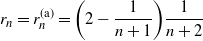








Figure 1 shows the path of
 $\lVert f_0 - f_n^\alpha\rVert_1$
. It takes about 150 iterations of PR for the
 $L^1$
-distance to stabilize.
 $||f_0 - f_n^{\alpha}||_1$
.

Figures 2(a)– 2(d) show the path of
 $\lVert f_0 - f_n^\beta\rVert_1$
for scenarios (i)–(iv) respectively. In the first case, it takes about 4000 iterations of PR for the
 $L^1$
-distance to stabilize. Thus, either
 $\beta_n$
does not converge in total variation or it does so more slowly than in scenarios (ii) and (iii). Indeed, in Figures 2(b) and 2(c) the
 $L_1$
-distance stabilizes quickly, which is consistent with the results that guarantee convergence in total variation in those cases (respectively, Theorem 3 and [Reference Fong, Holmes and Walker14, Theorem 5]). Figure 2(d) suggests lack of convergence in total variation, which is in line with Example 4.
 $||f_0 - f_n^{\beta}||_1$
.

A couple of remarks are in order. Firstly, we have seen that the choice of
 $r_n$
and
 $\rho$
in the
 $\beta_n$
significantly affects the reconstruction of uncertainty. This highlights what stated at the end of the previous section, i.e. that when making inference via PR we should also care about the updating mechanism of the predictives. For the
 $\beta_n$
with
 $c_n = c_{\rho}$
, some guidelines are provided in [Reference Fong, Holmes and Walker14] for choosing
 $r_n$
(as mentioned in this section) and
 $\rho$
. Thus, we follow them in the next section.
Secondly, Figures 2(a)– 2(c) show that
 $f_n^{\alpha}$
moves further from
 $f_0$
than
 $f_n^{\beta}$
does. This hints that
 $\alpha_n$
might reconstruct more uncertainty than
 $\beta_n$
, which would be consistent with the posterior variance estimates obtained in the next section.
3.3. Parameter estimation
We now compare
 $\alpha_n$
and
 $\beta_n$
when used to estimate the posterior distribution
 $\Pi_N({\cdot}\mid x)$
of some parameter
 $\theta$
via PR; see Section 3.1. We assume an initial dataset
 $x=(x_1,\ldots,x_s)$
is available and we build the predictives to account for it. Indeed, since we are performing PR,
 $\alpha_0$
should fit x. Similarly, the updating mechanism of the sequence
 $(\alpha_n)$
should preserve the information provided by x. The same remarks apply to
 $(\beta_n)$
.
The
 $\alpha_n$
are specified as follows. We partition x with a model-based clustering technique, available in the mclust R package [Reference Fraley and Raftery16–Reference Fraley, Raftery, Murphy and Scrucca18], which finds the mixture of Gaussians that best fits x, accounting also for model complexity, and the partition of x which most likely was induced by such mixture. Thus,
 $x = (x_{1,1},\ldots,x_{1,n_1},\ldots,x_{k,1},\ldots,x_{k,n_k})$
, where k is the number of clusters,
 $x_{i,j}$
is the jth observation of cluster i,
 $n_i$
is the size of cluster i, and
 $\sum_{i=1}^k n_i = s$
. Then, for
 $i=1,\ldots,k$
, we let
 $$a_i = \frac{1}{n_i}\sum_{j=1}^{n_i} x_{i,j},\qquad b_i = \frac{1}{n_i}\sum_{j=1}^{n_i} (x_{i,j}-a_i)^2,\qquad w_i = \frac{n_i}{s},$$
and Y be a random variable with distribution
 $m = \sum_{i=1}^k w_i \mathcal{N}(a_i,b_i)$
. Finally, the kernel
 $\mathcal{L}$
is chosen as the law of the random variable
 $(Y - \mathbb{E}(Y))/\sqrt{\mathrm{Var}(Y)}$
and the
 $\alpha_n$
are defined by (3).
Similarly to
 $\alpha_0$
,
 $\beta_0$
is constructed as an estimate of the density of the distribution that
 $x_1,\ldots,x_s$
are drawn from (x is assumed to be an i.i.d. sample; see below). Following [Reference Fong, Holmes and Walker14], this is done via prequential log-likelihood optimization. In particular, let
 $f_{n,\rho}^{\beta}$
be the density of
 $\beta_n$
for
 $\beta_0 = \mathcal{N}(0,1)$
,
 $c_n = c_{\rho}$
, and
 $r_n = r_n^\mathrm{(a)}$
. Then, we evaluate
 $f_{i-1,\rho}^{\beta}(x_i \mid x_1,\ldots,x_{i-1})$
for
 $i=1,\ldots,s$
and
 $\rho \in \{0.05,0.1,\ldots,0.95\}$
, and let
 $$\hat{\rho} = \operatorname*{arg\,max}_{\rho} \sum_{i=1}^s \log f_{i-1,\rho}^{\beta}(x_i \mid x_1,\ldots,x_{i-1}).$$
Finally, we set
 $\beta_0({\mathrm{d}}y) = f_{s,\hat{\rho}}^{\beta}(y\mid x)\,{\mathrm{d}}y$
. The rest of the sequence
 $(\beta_n)$
follows from the construction given in Section 2.3, upon setting
 $c_n = c_{\hat{\rho}}$
and
 $r_n = r_n^\mathrm{(a)}$
.
The parameter
 $\theta$
is taken as the mean, variance, skewness, kurtosis, and median of a reference population. In what follows,
 $\hat{\theta}$
is short for
 $\hat{\theta}(x,X_{1},\ldots,X_{N})$
, which represents the sample equivalent of the corresponding population quantity (e.g., if
 $\theta$
is the population mean,
 $\hat{\theta}$
is the sample mean). Moreover, when necessary we use the notations
 $\Pi_N^\alpha({\cdot}\mid x)$
and
 $\Pi_N^\beta({\cdot}\mid x)$
to stress that
 $\Pi_N({\cdot}\mid x)$
is obtained using the
 $\alpha_n$
or the
 $\beta_n$
.
The simulation study is organized as follows. We draw random samples of size
 $s = 50, 100, 500, 1000, 1500, 2000$
from a mixture of three shifted t-distributions with weights
 $w_1 = 0.3$
,
 $w_2 = 0.1$
, and
 $w_3 = 0.6$
, shifting constants
 $\mu_1 = -5$
,
 $\mu_2 = 0$
, and
 $\mu_3 = 4$
, and degrees of freedom
 $\nu = 4.5$
. Then, we run PR with
 $N = 5000$
and
 $B = 1000$
.
 $B = 1000$
allows us to visualize well posterior density and does not make PR too slow. Similarly,
 $N = 5000$
allows a satisfying compromise between computational speed and reconstruction of uncertainty. Once a sample
 $\boldsymbol{\theta} = (\theta_1,\ldots,\theta_B)$
from
 $\Pi_N({\cdot}\mid x)$
is obtained, we compute the root mean square error (RMSE) between
 $\boldsymbol{\theta}$
and the true parameter value (say
 $\theta_0$
) and the sample variance of
 $(\theta_1,\ldots,\theta_B)$
(which is an estimate of posterior variance). These indicators quantify how close
 $\Pi_N({\cdot}\mid x)$
is to
 $\theta_0$
and how much posterior uncertainty is generated by PR. We also keep track of computation times.
Tables 1 and 2 show the RMSE respectively for
 $\alpha_n$
and
 $\beta_n$
, while Tables 3 and 4 show the posterior variance. Overall, estimates appear to be more precise and less dispersed as s increases. This seems reasonable, as a larger sample size typically implies more information and less uncertainty. Averaging the RMSE values in Tables 1 and 2 over all sample sizes and parameters yields a mean RMSE of 0.818 and 2.731 respectively. One might think this discrepancy is due to
 $\Pi_N^{\beta}({\cdot} \mid x)$
being more dispersed than
 $\Pi_N^{\alpha}({\cdot} \mid x)$
, but Tables 3 and 4 provide opposing evidence. Indeed, averaging the values of those tables, we obtain a mean posterior variance of 0.206 for
 $\alpha_n$
and 0.019 for
 $\beta_n$
. Therefore, such a difference might be due to
 $\Pi_N^{\alpha}({\cdot} \mid x)$
being located on
 $\theta_0$
more often than
 $\Pi_N^{\beta}({\cdot} \mid x)$
. Evidence in favour of this can be found by looking at 95% credible intervals, estimated by taking sample quantiles of
 $(\theta_1,\ldots,\theta_B)$
. Indeed,
 $\beta_n$
tends to give rise to shorter intervals which contain
 $\theta_0$
less frequently. In particular, out of 30 different combinations of
 $\theta$
and s, the 95% credible intervals produced by
 $\alpha_n$
and
 $\beta_n$
contain
 $\theta_0$
respectively 15 and 3 times (see also Appendix B).
RMSE
 $\alpha_n$
.

Table 1 Long description
The table presents statistical measures for different values of s and theta. It has six columns labeled s = 50, s = 100, s = 500, s = 1000, s = 1500, and s = 2000. The rows are labeled Mean, Variance, Skewness, Kurtosis, and Median. Row 1: Mean, 2.055, 0.381, 0.341, 0.063, 0.009, 0.011. Row 2: Variance, 7.936, 3.149, 1.662, 0.646, 0.230, 0.103. Row 3: Skewness, 0.231, 0.018, 0.061, 0.009, 0.001, 0.001. Row 4: Kurtosis, 0.439, 0.178, 0.245, 0.002, 0.017, 0.037. Row 5: Median, 5.983, 0.382, 0.270, 0.022, 0.014, 0.055.
RMSE
 $\beta_n$
.

Table 2 Long description
A table with six columns and six rows, including a header row. The columns are labeled with different sample sizes (s = 50, s = 100, s = 500, s = 1000, s = 1500, s = 2000). The rows are labeled with statistical measures (Mean, Variance, Skewness, Kurtosis, Median). Each cell contains a numerical value corresponding to the statistical measure for the given sample size. The table provides a detailed comparison of how different statistical measures vary with sample size.
Posterior variance
 $\alpha_n$
.

Table 3 Long description
A table with six columns and seven rows, comparing statistical measures for different sample sizes (s = 50, s = 100, s = 500, s = 1000, s = 1500, s = 2000). The rows are labeled as Mean, Variance, Skewness, Kurtosis, and Median. Each cell contains a numerical value corresponding to the statistical measure for the given sample size. The table shows how these measures change as the sample size increases.
Posterior variance
 $\beta_n$
.

Table 4 Long description
A table with six columns and six rows, including a header row. The columns are labeled with different sample sizes (s = 50, s = 100, s = 500, s = 1000, s = 1500, s = 2000). The rows are labeled with statistical measures (Mean, Variance, Skewness, Kurtosis, Median). Each cell contains a numerical value corresponding to the statistical measure for the given sample size. Row 1: Mean, 0.003, 0.003, 0.004, 0.003, 0.002, 0.002. Row 2: Variance, 0.048, 0.053, 0.149, 0.105, 0.080, 0.084. Row 3: Skewness, 0.0004, 0.0004, 0.001, 0.001, 0.001, 0.001. Row 4: Kurtosis, 0.001, 0.001, 0.003, 0.003, 0.002, 0.002. Row 5: Median, 0.005, 0.005, 0.006, 0.005, 0.004, 0.006.
There might be a couple of ways to improve the performance of
 $\beta_n$
. Firstly, we could take a finer grid of candidate values of
 $\rho$
for the prequential log-likelihood optimisation. In this way,
 $\beta_0$
should fit better the observed data and thus make estimates more precise. Secondly, we could make the sampling mechanism more accurate. Indeed,
 $X_{1},\ldots,X_{N}$
are generated via inverse sampling from a grid
 $\{y_1,\ldots,y_G\}$
. Thus, once again, better posterior estimates could be obtained by refining such a grid. It is worth stressing that, if one wants only to update
 $\beta_n$
into
 $\beta_{n+1}$
, it is not necessary to sample
 $X_{n+1} \sim \beta_n$
and plug it in to
 $\beta_{n+1}$
. As explained in [Reference Fong, Holmes and Walker14, Section 4.2], it is enough to draw an observation from a uniform distribution on (0, 1). But clearly, we cannot use this shortcut for we need to know the actual value of the sampled variables. Finally, we note that these ameliorations come at the cost of longer computation times. We explore this further in the next paragraph.
Table 5 shows the time needed to perform PR for
 $\alpha_n$
,
 $\beta_n$
, and each value of s. The PR algorithm is coded in Rcpp. Computations are carried out on a single-core version of R installed on a machine with an AMD Epyc 7763 2.45 Ghz processor with 2 TB RAM. The difference between the computation times of
 $\alpha_n$
and
 $\beta_n$
, with the former being much faster than the latter, is quite evident. Reasons for this discrepancy have partially been pointed out already, so we summarize them and provide some more details. Sampling from
 $\alpha_n$
requires just computing a mean, a variance, drawing one of the components of the Gaussian mixture (with probability equal to its weight), and then sampling from it. This can be done efficiently in any statistical software. On the other hand, sampling from
 $\beta_n$
entails estimating the hyperparameter
 $\rho$
(at the beginning of PR) and doing inverse sampling. The time needed for these tasks depends on the size of the grid of values taken to perform them. Such a grid cannot be too coarse, otherwise the accuracy of the estimates is worsened. Therefore, these two steps are likely to be the main reason why
 $\alpha_n$
is faster than
 $\beta_n$
. Furthermore, computational times for
 $\beta_n$
increase significantly with sample size. This might be due to the estimation of
 $\rho$
being affected by s. Indeed, as explained at the beginning of this section, optimizing the prequential log-likelihood requires a recursive evaluation of the predictive density from step 0 to s, for each candidate value of
 $\rho$
. Clearly, this procedure is slower the larger the value of s. Even the performance of
 $\alpha_n$
is affected by s, which is likely due to model-based clustering being slower the larger the sample to partition. Yet, the impact is way less marked.
Computation times in minutes.

Table 5 Long description
A table with six columns and two rows. The columns are labeled with different values of s: 50, 100, 500, 1000, 1500, and 2000. The rows are labeled with alpha_n and beta_n. Row 1: alpha_n, 0.012, 0.014, 0.017, 0.021, 0.022, 0.026. Row 2: beta_n, 5.10, 5.87, 7.12, 8.26, 8.28, 9.98.
4. Discussion
Let
 $X=(X_1,X_2,\ldots)$
be a sequence of p-dimensional random vectors, and
 $$\alpha_n({\cdot})=\mathbb{P}\bigl(X_{n+1}\in{\cdot}\mid X_1,\ldots,X_n\bigr)$$
the corresponding predictive distributions. In this paper, a new sequence
 $(\alpha_n)$
of predictives is introduced, namely
 $\alpha_n = \mathcal{L}(M_n,Q_n)$
, where
 $\mathcal{L}$
is a suitable kernel, and
 $M_n$
and
 $Q_n$
are the sample mean and covariance matrix of
 $(X_1,\ldots,X_n)$
. Convergence in total variation of
 $\alpha_n$
is proved, along with an explicit formula for the limit RPM. In the (meaningful) special case where
 $\mathcal{L} = \mathcal{N}$
, the convergence rate is shown to be
 $n^{-1/2}$
. A natural competitor of
 $\alpha_n$
is the copula-based predictive distribution
 $\beta_n$
of [Reference Hahn, Martin and Walker19]. Thus,
 $\beta_n$
is investigated as well. It turns out that
 $\beta_n$
converges weakly but not necessarily in total variation. Hence, sufficient conditions for
 $\beta_n$
to converge in total variation are provided. Eventually, an empirical comparison between
 $\alpha_n$
and
 $\beta_n$
is performed, assessing their speed of convergence and their ability to estimate, via PR, the posterior distribution of population moments and quantiles.
When making parameter inference,
 $\mathcal{L}$
is chosen as a mixture of Gaussians retrieved via model-based clustering on the initial dataset x. This flexible structure allows us to capture well the shape and location of the underlying population, as demonstrated by the satisfying performance of
 $\alpha_n$
in PR.
We finally mention two issues for future research. The first is to give conditions on
 $\mathcal{L}$
under which the convergence rate of
 $\alpha_n$
is still
 $n^{-1/2}$
(as happens when
 $\mathcal{L}=\mathcal{N}$
). The second is using the
 $\alpha_n$
in regression problems (as done in [Reference Fong, Holmes and Walker14] with the
 $\beta_n$
). In this case, the data are of the type
 $X_n=(Y_n,Z_n)$
, where
 $Y_n$
is a response variable and
 $Z_n$
a vector of covariates. Thus, one could generate several multivariate populations via PR and then use standard frequentist estimators to obtain a posterior sample of regression functions.
Appendix A. Proofs
In this appendix, we prove the results of Section 2. To this end, we first recall two known facts and we make a preliminary remark.
Lemma 1. If
 $x,y\in\mathbb{R}^p$
and B is a real non-singular matrix of order
 $p\times p$
, then
 $$\operatorname{det}\bigl(B+xy^{\top})=\operatorname{det}(B)\bigl(1+x^{\top} b^{-1}y\bigr).$$
Lemma 2. If
 $(V_n\colon n\ge 1)$
is an i.i.d. sequence of real random variables such that
 $\mathbb{E}(V_1)=0$
and
 $\mathbb{E}\bigl(\lvert V_1\rvert^{1+\varepsilon}\bigr)<\infty$
for some
 $\varepsilon>0$
, then the series
 $\sum_{n=1}^\infty{V_n}/{n}$
converges a.s.
Proof. Since
 $\sum_n\mathbb{P}(\lvert V_n\rvert>n) = \sum_n\mathbb{P}(\lvert V_1\rvert>n) \le \mathbb{E}\bigl(\lvert V_1\rvert\bigr)<\infty$
, the Borel–Cantelli lemma yields
 $\mathbb{P}(\lvert V_n\rvert>n$
for infinitely many
 $n)=0$
. Hence, it suffices to show that
 $\sum_n{W_n}/{n}$
converges a.s., where
 $W_n=V_n\mathbf{1}_{\{\lvert V_n\rvert\le n\}}$
. To this end, first note that
 $({W_n-\mathbb{E}(W_n)})/{n}$
are independent and centered, and
 $$ \sum_n\mathbb{E}\bigg\{\bigg(\frac{W_n-\mathbb{E}(W_n)}{n}\bigg)^2\bigg\} \le \sum_n\mathbb{E}\bigg\{\frac{V_1^2\mathbf{1}_{\{\lvert V_1\rvert\le n\}}}{n^2}\bigg\} \le \sum_n\frac{\mathbb{E}\bigl(\lvert V_1\rvert^{1+\varepsilon}\bigr)}{n^{1+\varepsilon}}<\infty. $$
Hence, the series
 $\sum_n({W_n-\mathbb{E}(W_n)})/{n}$
converges a.s. Finally,
 $\mathbb{E}(V_1)=0$
implies
 $$ \mathbb{E}(W_n) = \mathbb{E}\bigl\{V_1\mathbf{1}_{\{\lvert V_1\rvert\le n\}}\bigr\} = -\mathbb{E}\bigl\{V_1\mathbf{1}_{\{\lvert V_1\rvert> n\}}\bigr\}. $$
Therefore,
 $$ \sum_n\frac{\lvert\mathbb{E}(W_n)\rvert}{n} \le \sum_n\frac{\mathbb{E}\bigl\{\lvert V_1\rvert\mathbf{1}_{\{\lvert V_1\rvert> n\}}\bigr\}}{n} \le \sum_n\frac{\mathbb{E}\bigl(\lvert V_1\rvert^{1+\varepsilon}\bigr)}{n^{1+\varepsilon}}<\infty. $$
This concludes the proof.
Both the previous lemmas are well known. A possible reference for Lemma 1 is [Reference Ding and Zhou11], while Lemma 2 has been proved here as we know of no explicit reference. Incidentally, in Lemma 2, the condition
 $\mathbb{E}\bigl(\lvert V_1\rvert^{1+\varepsilon}\bigr)<\infty$
can possibly be weakened but not completely removed. In fact, as shown in the next example, the series
 $\sum_{n=1}^\infty{V_n}/{n}$
may fail to converge a.s. even if
 $(V_n)$
is i.i.d. and
 $\mathbb{E}(V_1)=0$
.
Example 5. Let
 $(V_n)$
be i.i.d. with
 $\mathbb{P}(V_1=-c/\log 2)=\frac12$
and
 $$\mathbb{P}(2<V_1\le x)=\frac{c}{2}\int_2^x\frac{{\mathrm{d}}t}{(t\log t)^2} \quad \text{for }x>2,$$
where the constant c is given by
 $c=\bigl(\int_2^\infty{{\mathrm{d}}t}/{(t\log t)^2})^{-1}$
. Then,
 $$\mathbb{E}(V_1)=-\bigg\{\frac{c}{2\log 2}+\frac{c}{2}\bigg\}\int_2^\infty\frac{t}{(t\log t)^2}\,{\mathrm{d}}t=0.$$
Letting
 $W_n=({V_n}/{n})\mathbf{1}_{\{\lvert V_n\rvert\le n\}}$
, a direct calculation shows that we have
 $\sum_n\mathbb{E}(W_n)=-\infty$
and
 $\sum_n\operatorname{Var}(W_n)<\infty$
. Hence,
 $\sum_{n=1}^\infty W_n\overset{\mathrm{a.s.}}=-\infty$
. In turn, by the Borel–Cantelli lemma, this implies that
 $\sum_{n=1}^\infty{V_n}/{n}\overset{\mathrm{a.s.}}=-\infty$
.
Remark 3. In order to prove Theorems 1 and 2, without loss of generality, some simplifications are admissible. Firstly, the
 $\alpha_n$
can be assumed to be as in Remark 2, i.e.
 \begin{equation} \begin{gathered} \alpha_0=\mathcal{L}(0,I), \qquad \alpha_1=\mathcal{L}(X_1,I), \qquad \alpha_n=\mathcal{L}(M_n,Q_n)\quad\text{for }n\ge 2, \\ \text{where} \quad M_n=\frac{\sum_{i=1}^nX_i}{n}, \qquad Q_n=\frac{\sum_{i=1}^n(X_i-M_n)(X_i-M_n)^{\top}}{n}. \end{gathered} \end{equation}
Secondly, the
 $X_n$
can be defined as follows. Fix an i.i.d. sequence
 $Z_1,Z_2,\ldots$
of p-dimensional random vectors such that
 $Z_1\sim\mathcal{L}(0,I)$
. Define a sequence
 $Y=(Y_1,Y_2,\ldots)$
as
 \begin{gather*} Y_1=Z_1, \qquad Y_2=Y_1+Z_2, \qquad Y_{n+1}=N_n+R_n^{1/2}Z_{n+1} \quad \text{for }n\ge 2, \\ \text{where} \quad N_n=\frac{1}{n}\sum_{i=1}^nY_i, \qquad R_n=\frac{1}{n}\sum_{i=1}^n(Y_i-N_n)(Y_i-N_n)^{\top}. \end{gather*}
It is straightforward to see that
 $\mathbb{P}(Y_1\in{\cdot})=\mathcal{L}(0,I)$
,
 $\mathbb{P}(Y_2\in{\cdot}\mid Y_1)=\mathcal{L}(Y_1,I)$
, and that
 $\mathbb{P}(Y_{n+1}\in{\cdot}\mid Y_1,\ldots,Y_n)=\mathcal{L}(N_n,R_n)$
for
 $n\ge 2$
. Hence,
 $Y\sim X$
whenever the predictive distributions of X are given by (9). In particular, since
 $Y\sim X$
, in the proofs of Theorems 1 and 2 we can suppose that
 $X_1=Z_1$
,
 $X_2=X_1+Z_2$
, and
 $X_{n+1}=M_n+Q_n^{1/2}Z_{n+1}$
for
 $n\ge 2$
, where
 $Z_1,Z_2,\ldots$
are i.i.d. and
 $Z_1\sim\mathcal{L}(0,I)$
.
We are now able to attack the results of Section 2.2. To this end, we let
 $\mathcal{F}_n=\sigma(Z_1,\ldots,Z_n)$
, with
 $\mathcal{F}_0$
the trivial
 $\sigma$
-field.
Proof of Theorem
1
. Suppose
 $M_n\overset{\textrm{a.s.}}\longrightarrow M$
,
 $Q_n\overset{\textrm{a.s.}}\longrightarrow Q$
, and
 $Q\in\mathcal{M}$
a.s. Let
 $\phi$
be a density of
 $\mathcal{L}(0,I)$
with respect to p-dimensional Lebesgue measure. For each
 $n\ge 1$
, under the predictives
 $\alpha_0,\alpha_1,\ldots,\alpha_{n-1}$
, the probability distribution of
 $(X_1,\ldots,X_n)$
is absolutely continuous with respect to np-dimensional Lebesgue measure. Based on this fact, by standard arguments, it can be easily seen that
 $Q_n\in\mathcal{M}$
a.s. Therefore,
 \begin{equation*} \lVert\alpha_n-\alpha\rVert = \lVert\mathcal{L}(M_n,Q_n)-\mathcal{L}(M,Q)\rVert \overset{\mathrm{a.s.}}= \frac{1}{2}\int_{\mathbb{R}^p}\biggl\lvert\frac{\phi\bigl(Q_n^{-1/2}(x-M_n)\bigr)}{\text{det}(Q_n)^{1/2}} - \frac{\phi\bigl(Q^{-1/2}(x-M)\bigr)}{\text{det}(Q)^{1/2}}\biggr\rvert\,{\mathrm{d}}x. \end{equation*}
Given
 $\varepsilon>0$
, take an integrable continuous function f on
 $\mathbb{R}^p$
such that
 $\int_{\mathbb{R}^p}\lvert\phi(x)-f(x)\rvert\,{\mathrm{d}}x<\varepsilon$
. Define
 \begin{gather*} I_n = \int_{\mathbb{R}^p}\biggl\lvert\frac{f\bigl(Q_n^{-1/2}(x-M_n)\bigr)}{\text{det}(Q_n)^{1/2}} - \frac{f\bigl(Q^{-1/2}(x-M)\bigr)}{\text{det}(Q)^{1/2}}\biggr\rvert\,{\mathrm{d}}x. \end{gather*}
Since f is continuous,
 $I_n\overset{\textrm{a.s.}}\longrightarrow 0$
. Therefore,
 $\limsup_n\lVert\alpha_n-\alpha\rVert\le\varepsilon+\frac{1}{2}\limsup_nI_n\overset{a.s.}=\varepsilon$
. This proves that
 $\lVert\alpha_n-\alpha\rVert\overset{\textrm{a.s.}}\longrightarrow 0$
provided
 $M_n\overset{\textrm{a.s.}}\longrightarrow M$
,
 $Q_n\overset{\textrm{a.s.}}\longrightarrow Q$
, and
 $Q\in\mathcal{M}$
a.s.
After noting this fact, the rest of the proof is split into three steps. Recall that, by Remark 3, we can assume
 $X_1=Z_1$
,
 $X_2=X_1+Z_2$
, and
 $X_{n+1}=M_n+Q_n^{1/2}Z_{n+1}$
for
 $n\ge 2$
, where
 $Z_1,Z_2,\ldots$
are i.i.d. and
 $Z_1\sim\mathcal{L}(0,I)$
.
Step 1:
 $Q_n$
converges a.s. Define
 $M_0=0$
,
 $Q_0=Q_1=I$
, and
 $L_n=Q_n^{1/2}Z_{n+1}$
. Then
 $$M_{n+1}-M_n=\frac{Q_n^{1/2}Z_{n+1}}{n+1}=\frac{L_n}{n+1}.$$
After some algebra, this implies that
 \begin{gather} Q_{n+1}=\frac{n}{n+1}Q_n+\frac{n}{(n+1)^2}L_nL_n^{\top}, \end{gather}
or, equivalently,
 $$Q_{n+1}^{(i,j)}=\frac{n}{n+1}Q_n^{(i,j)}+\frac{n}{(n+1)^2}L_n^{(i)}L_n^{(j)}\quad\text{for all }i,j=1,\ldots,p.$$
The conditional distribution of
 $L_n$
given
 $\mathcal{F}_n$
is
 $\mathcal{L}(0,Q_n)$
. Therefore,
 $\mathbb{E}\bigl\{L_n^{(i)}\,L_n^{(j)}\mid\mathcal{F}_n\bigr\}=Q_n^{(i,j)}$
and
 \begin{gather*} \mathbb{E}\bigl\{Q_{n+1}^{(i,j)}\mid\mathcal{F}_n\bigr\} = \frac{n}{n+1}Q_n^{(i,j)} + \frac{n}{(n+1)^2}Q_n^{(i,j)} = Q_n^{(i,j)}\bigg(1-\frac{1}{(n+1)^2}\bigg). \end{gather*}
For
 $i=j$
, it follows that
 $(Q_n^{(i,i)}\colon n\ge 2)$
is a non-negative supermartingale. Hence,
 $$\mathbb{E}\bigl\{\lvert Q_n^{(i,j)}\rvert\bigr\} \le \frac{\mathbb{E}\bigl\{Q_n^{(i,i)}\bigr\}+\mathbb{E}\bigl\{Q_n^{(j,j)}\bigr\}}{2} \le \frac{\mathbb{E}\bigl\{Q_2^{(i,i)}\bigr\}+\mathbb{E}\bigl\{Q_2^{(j,j)}\bigr\}}{2}$$
and
 \begin{align*} \sum_n\mathbb{E}\bigl\lvert\mathbb{E}\bigl\{Q_{n+1}^{(i,j)}\mid\mathcal{F}_n\bigr\}-Q_n^{(i,j)}\bigr\rvert & = \sum_n\frac{\mathbb{E}\bigl\{\lvert Q_n^{(i,j)}\rvert\bigr\}}{(n+1)^2} \\ & \le \frac{\mathbb{E}\bigl\{Q_2^{(i,i)}\bigr\}+\mathbb{E}\bigl\{Q_2^{(j,j)}\bigr\}}{2} \sum_n\frac{1}{(n+1)^2} < \infty. \end{align*}
To sum up, for fixed i and j, the sequence
 $(Q_n^{(i,j)}\colon n\ge 2)$
is a quasi-martingale such that
 $\sup_n\mathbb{E}\bigl\{\lvert Q_n^{(i,j)}\rvert\bigr\}<\infty$
, and this implies that
 $Q_n^{(i,j)}\overset{\mathrm{a.s.}}\longrightarrow Q^{(i,j)}$
for some random variable
 $Q^{(i,j)}$
. Hence,
 $Q_n\overset{\mathrm{a.s.}}\longrightarrow Q$
, where Q is the matrix
 $Q=\bigl(Q^{(i,j)}\colon 1\le i,j\le p\bigr)$
.
Step 2:
 $M_n$
is a martingale and it is bounded in
 $L_2$
. Just note that
 \begin{equation*} \mathbb{E}(M_{n+1}-M_n\mid\mathcal{F}_n) = \mathbb{E}\bigg\{\frac{Q_n^{1/2}Z_{n+1}}{n+1}\mid\mathcal{F}_n\bigg\} = \frac{Q_n^{1/2}\mathbb{E}(Z_{n+1}\mid\mathcal{F}_n)}{n+1} = \frac{Q_n^{1/2}\mathbb{E}(Z_{n+1})}{n+1} = 0. \end{equation*}
Hence,
 $M_n$
is a martingale. In addition,
 \begin{align*} \mathbb{E}(M_n^{\top} M_n) & = \mathbb{E}\Bigg\{\Bigg(\sum_{i=1}^n\frac{Q_{i-1}^{1/2}Z_i}{i}\Bigg)^{\top} \Bigg(\sum_{j=1}^n\frac{Q_{j-1}^{1/2}Z_j}{j}\Bigg)\Bigg\} \\ & = \sum_{i=1}^n\frac{\mathbb{E}\big(Z_i^{\top} Q_{i-1}Z_i\big)}{i^2} \\ & = \sum_{i=1}^n\sum_{r,k=1}^p\frac{\mathbb{E}\big(Z_i^{(r)}Z_i^{(k)}\big)\mathbb{E}\big(Q_{i-1}^{(r,k)}\big)}{i^2} \\ & = \sum_{i=1}^n\sum_{k=1}^p\frac{\mathbb{E}\big(Q_{i-1}^{(k,k)}\big)}{i^2} \\ & \le \sum_{i=1}^\infty\sum_{k=1}^p\frac{\mathbb{E}\big(Q_{i-1}^{(k,k)}\big)}{i^2} \le p + \frac{p}{4} + \sum_{k=1}^p\mathbb{E}\big(Q_2^{(k,k)}\big)\sum_{i=3}^\infty\frac{1}{i^2}, \end{align*}
where the last inequality is because
 $(Q_n^{(k,k)}\colon n\ge 2)$
is a supermartingale for fixed
 $k=1,\ldots,p$
. Therefore,
 $M_n$
is a martingale such that
 $\sup_n\mathbb{E}(M_n^{\top} M_n)<\infty$
, and this implies that
 $M_n\overset{\mathrm{a.s.}}\longrightarrow M$
for some p-dimensional random vector M.
Step 3:
 $Q\in\mathcal{M} $
a.s. Since
 $Q\overset{\mathrm{a.s.}}=\lim_nQ_n$
, the matrix Q is symmetric and non-negative definite a.s. Hence, to prove
 $Q\in\mathcal{M}$
a.s., it suffices to show that
 $\operatorname{det}(Q)>0$
a.s.
Exploiting (10) and Lemma 1, we obtain
 \begin{align*} \operatorname{det}(Q_{n+1}) & = \operatorname{det}\bigg(\frac{n}{n+1}Q_n^{1/2}\bigg(I+\frac{1}{(n+1)}\,Z_{n+1}Z_{n+1}^{\top}\bigg)Q_n^{1/2}\bigg)\\ & = \operatorname{det}(Q_n)\bigg(1-\frac{1}{n+1}\bigg)^p\bigg(1+\frac{1}{n+1}Z_{n+1}^{\top} Z_{n+1}\bigg). \end{align*}
Letting
 $V_n=Z_n^{\top} Z_n-p$
, the above equation can be written as
 \begin{align*} \operatorname{det}(Q_{n+1}) & = \operatorname{det}(Q_n)\sum_{j=0}^p \begin{pmatrix} p \\ j \end{pmatrix} \bigg(\frac{-1}{n+1}\bigg)^j\bigg(1+\frac{V_{n+1}+p}{n+1}\bigg) \\ & = \operatorname{det}(Q_n)\bigg\{1+\frac{V_{n+1}}{n+1}-p\frac{V_{n+1}+p}{(n+1)^2}+R_{n+1}\bigg\}, \end{align*}
where
 $$R_{n+1} = \sum_{j=2}^p \begin{pmatrix} p \\ j \end{pmatrix} \bigg(\frac{-1}{n+1}\bigg)^j\bigg(1+\frac{V_{n+1}+p}{n+1}\bigg).$$
Therefore,
 $$ \operatorname{det}(Q_n) = \operatorname{det}(Q_2)\prod_{j=3}^n\frac{\operatorname{det}(Q_j)}{\operatorname{det}(Q_{j-1})} = \operatorname{det}(Q_2)\prod_{j=3}^n\bigg\{1+\frac{V_j}{j}-p\frac{V_j+p}{j^2}+R_j\bigg\}. $$
Next, define
 $$U_j=1+\frac{V_j}{j}-p\frac{V_j+p}{j^2}+R_j.$$
If
 $\sum_{j=3}^n\log U_j\overset{\mathrm{a.s.}}\longrightarrow T$
as
 $n\rightarrow\infty$
for some real random variable T, then
 $$\operatorname{det}(Q) = \lim_n\operatorname{det}(Q_n) = \operatorname{det}(Q_2)\lim_n\exp\Bigg(\sum_{j=3}^n\log U_j\Bigg) = \operatorname{det}(Q_2){\mathrm{e}}^T>0 \quad \text{a.s.}$$
Hence, it suffices to show that the series
 $\sum_j\log U_j$
converges a.s. In turn, this is true since each series involved in the definition of
 $U_j$
converges a.s. Precisely,
 $\sum_j{V_j}/{j}$
converges a.s. because of Lemma 2. The series
 $\sum_j({V_j+p})/{j^2}$
converges a.s. since
 $V_j+p=Z_j^{\top} Z_j\ge 0$
and
 $$ \mathbb{E}\Bigg\{\sum_j\frac{V_j+p}{j^2}\Bigg\} = \sum_j\frac{\mathbb{E}(Z_j^{\top} Z_j)}{j^2} = \sum_j\frac{p}{j^2} < \infty. $$
Finally,
 $\sum_jR_j$
converges a.s. by exactly the same argument as used for
 $\sum_j({V_j+p})/{j^2}$
. Therefore,
 $\sum_j\log U_j$
converges a.s., and this concludes the proof.
Proof of Theorem
2
. Let
 $\lVert{\cdot}\rVert_\mathrm{E}$
be the Euclidean norm on
 $\mathbb{R}^p$
, and
 $\lVert{\cdot}\rVert_\mathrm{F}$
the Frobenius norm on the matrices of order
 $p\times p$
. The latter is defined as
 $\lVert B\rVert_\mathrm{F}=\sqrt{\sum_{i,j}(B^{(i,j)})^2}=\sqrt{\operatorname{trace}(B^{\top} B)}$
for any
 $p\times p$
matrix B and has the nice property that
 $\lVert B_1B_2\rVert_\mathrm{F}\le\lVert B_1\rVert_\mathrm{F}\lVert B_2\rVert_\mathrm{F}$
.
The total variation distance between two p-dimensional normal laws, say
 $\mathcal{N}(a,\Sigma_1)$
and
 $\mathcal{N}(b,\Sigma_2)$
with
 $a,b\in\mathbb{R}^p$
and
 $\Sigma_1,\Sigma_2\in\mathcal{M}$
, can be estimated as
 $$ \lVert\mathcal{N}(a,\Sigma_1) - \mathcal{N}(b,\Sigma_2)\rVert \le \lVert\mathcal{N}(a,\Sigma_1) - \mathcal{N}(b,\Sigma_1)\rVert + \tfrac{3}{2}\big\lVert\Sigma_1^{-1/2}\Sigma_2\Sigma_1^{-1/2}-I\big\rVert_\mathrm{F}; $$
see, e.g., [Reference Kelbert22, Theorem 2] and [Reference Devroye, Mehrabian and Reddad10, (2)]. In addition,
 $$ \big\lVert\Sigma_1^{-1/2}\Sigma_2\Sigma_1^{-1/2}-I\big\rVert_\mathrm{F} = \big\lVert\Sigma_1^{-1/2}(\Sigma_2-\Sigma_1)\Sigma_1^{-1/2}\big\rVert_\mathrm{F} \le \big\lVert\Sigma_1^{-1/2}\big\rVert_\mathrm{F}^2\lVert\Sigma_2-\Sigma_1\rVert_\mathrm{F} $$
and
 $\lVert\mathcal{N}(a,\Sigma_1)-\mathcal{N}(b,\Sigma_1)\rVert \le \lVert b-a\rVert_\mathrm{E}\big\lVert\Sigma_1^{-1/2}\big\rVert_\mathrm{F}$
; see [Reference Devroye, Mehrabian and Reddad10, p. 5]. Collecting all these facts together,
 $\lVert\mathcal{N}(a,\Sigma_1)-\mathcal{N}(b,\Sigma_2)\rVert \le C(\Sigma_1)\bigl\{\lVert b-a\rVert_\mathrm{E}+\lVert\Sigma_2-\Sigma_1\rVert_\mathrm{F}\bigr\}$
, where
 $C(\Sigma_1)$
is a constant that depends on
 $\Sigma_1$
only.
Applying the previous inequality to our framework, we obtain
 $$ \lVert\alpha_n-\alpha\rVert = \lVert\mathcal{N}(M_n,Q_n)-\mathcal{N}(M,Q)\rVert \le C(Q)\{\lVert M_n-M\rVert_\mathrm{E}+\lVert Q_n-Q\rVert_\mathrm{F}\}. $$
Hence, it suffices to show that
 $b:=\sup_n\sqrt{n}\mathbb{E}\{\lVert M_n-M\rVert_\mathrm{E}+\lVert Q_n-Q\rVert_\mathrm{F}\}<\infty$
. In fact, if
 $b<\infty$
and
 $d_n$
is any sequence of constants such that
 ${d_n}/{\sqrt{n}}\rightarrow 0$
, then
 $$ d_n\mathbb{E}\{\lVert M_n-M\rVert_\mathrm{E}+\lVert Q_n-Q\rVert_\mathrm{F}\} \le \frac{bd_n}{\sqrt{n}}\longrightarrow 0. $$
In particular,
 $d_n\{\lVert M_n-M\rVert_\mathrm{E}+\lVert Q_n-Q\rVert_\mathrm{F}\} \overset{\mathbb{P}}\longrightarrow 0$
, which in turn implies that
 $$ d_n\lVert\alpha_n-\alpha\rVert \le d_nC(Q)\{\lVert M_n-M\rVert_\mathrm{E}+\lVert Q_n-Q\rVert_\mathrm{F}\}\overset{\mathbb{P}}\longrightarrow 0. $$
To prove
 $b<\infty$
, we first note that
 $$M-M_n=\sum_{i=n}^\infty(M_{i+1}-M_i)=\sum_{i=n}^\infty\frac{Q_i^{1/2}Z_{i+1}}{i+1}.$$
Therefore, for each
 $n\ge 2$
,
 \begin{align*} \mathbb{E}\bigl\{\lVert M_n-M\rVert_\mathrm{E}\bigr\}^2 \le \mathbb{E}\bigl\{\lVert M_n-M\rVert_\mathrm{E}^2\bigr\} & = \mathbb{E}\bigl\{(M-M_n)^{\top}(M-M_n)\bigr\} \\ & = \sum_{i=n}^\infty\frac{\mathbb{E}\big(Z_{i+1}^{\top} Q_iZ_{i+1}\big)}{(i+1)^2} \\ & = \sum_{i=n}^\infty\sum_{r,k=1}^p \frac{\mathbb{E}\big(Z_{i+1}^{(r)}Z_{i+1}^{(k)}\big)\mathbb{E}\big(Q_i^{(r,k)}\big)}{(i+1)^2} \\ & = \sum_{i=n}^\infty\sum_{k=1}^p\frac{\mathbb{E}\big(Q_i^{(k,k)}\big)}{(i+1)^2} \le \sum_{k=1}^p\mathbb{E}(Q_2^{(k,k)})\sum_{i=n}^\infty\frac{1}{(i+1)^2}, \end{align*}
where the last inequality is because
 $\{Q_i^{(k,k)}\colon i\ge 2\}$
is a supermartingale for fixed k. On noting that
 $\sum_{i=n}^\infty{1}/{(i+1)^2}\le{1}/{n}$
, we obtain
 $$\sqrt{n}\mathbb{E}\bigl\{\lVert M_n-M\rVert_\mathrm{E}\bigr\} \le \sqrt{\sum_{k=1}^p\mathbb{E}\big(Q_2^{(k,k)}\big)}.$$
Similarly, recalling that
 $$Q_{n+1}=\frac{n}{n+1}Q_n^{1/2}\bigg(I+\frac{Z_{n+1}Z_{n+1}^{\top}}{n+1}\bigg)Q_n^{1/2},$$
we obtain
 \begin{gather*} Q-Q_n=\sum_{i=n}^\infty(Q_{i+1}-Q_i) = \sum_{i=n}^\infty\bigg\{\frac{Q_i^{1/2}\big(Z_{i+1}Z_{i+1}^{\top}-I\big)Q_i^{1/2}}{i+1} - \frac{Q_i^{1/2}Z_{i+1}Z_{i+1}^{\top} Q_i^{1/2}}{(i+1)^2}\bigg\}. \end{gather*}
Define
 $q=\sup_i\mathbb{E}\bigl\{\lVert Q_i^{1/2}\rVert_\mathrm{F}^4\bigr\}$
and
 $K_i={Q_i^{1/2}\big(Z_{i+1}Z_{i+1}^{\top}-I\big)Q_i^{1/2}}/({i+1})$
. Since
 $\mathbb{E}\bigl\{\lVert Q_i^{1/2}\rVert_\mathrm{F}^2\bigr\}\le\sqrt{q}$
for all i,
 \begin{align*} \sum_{i=n}^\infty\frac{\mathbb{E}\bigl\{\lVert Q_i^{1/2}Z_{i+1}Z_{i+1}^{\top} Q_i^{1/2}\rVert_\mathrm{F}\bigr\}}{(i+1)^2} & \le \sum_{i=n}^\infty\frac{\mathbb{E}\bigl\{\lVert Z_{i+1}Z_{i+1}^{\top}\rVert_\mathrm{F}\bigr\} \mathbb{E}\bigl\{\lVert Q_i^{1/2}\rVert_\mathrm{F}^2\bigr\}}{(i+1)^2} \\ & \le \mathbb{E}\bigl\{\lVert Z_1Z_1^{\top}\rVert_\mathrm{F}\bigr\} \sum_{i=n}^\infty\frac{\sqrt{q}}{(i+1)^2} \le \frac{\sqrt{q}}{n}\mathbb{E}\bigl\{\lVert Z_1Z_1^{\top}\rVert_\mathrm{F}\bigr\}. \end{align*}
Since
 $K_i$
is symmetric and
 $\mathbb{E}(K_iK_j)=0$
for
 $i\ne j$
,
 \begin{align*} \mathbb{E}\Bigg\{\Bigg\lVert\sum_{i=n}^\infty K_i\Bigg\rVert_\mathrm{F}^2\Bigg\} & = \mathbb{E}\Bigg\{\operatorname{trace}\Bigg(\Bigg(\sum_{i=n}^\infty K_i\Bigg) \Bigg(\sum_{j=n}^\infty K_j\Bigg)\Bigg)\Bigg\} \\ & = \operatorname{trace}\Bigg(\sum_{i,j=n}^\infty\mathbb{E}(K_iK_j)\Bigg) \\ & = \operatorname{trace}\Bigg(\sum_{i=n}^\infty\mathbb{E}(K_iK_i)\Bigg) \\ & = \sum_{i=n}^\infty\mathbb{E}\bigg\{ \frac{\lVert Q_i^{1/2}\big(Z_{i+1}Z_{i+1}^{\top}-I\big)Q_i^{1/2}\rVert_\mathrm{F}^2}{(i+1)^2}\bigg\} \\ & \le \mathbb{E}\bigl\{\lVert Z_1Z_1^{\top}-I\rVert_\mathrm{F}^2\bigr\} \sum_{i=n}^\infty\frac{\mathbb{E}\bigl\{\lVert Q_i^{1/2}\rVert_\mathrm{F}^4\bigr\}}{(i+1)^2} \le \mathbb{E}\bigl\{\lVert Z_1Z_1^t-I\rVert_\mathrm{F}^2\bigr\}\frac{q}{n}. \end{align*}
Hence,
 \begin{align*} \sqrt{n}\mathbb{E}\bigl\{\lVert Q_n-Q\rVert_\mathrm{F}\bigr\} & \le \sqrt{n}\sum_{i=n}^\infty \frac{\mathbb{E}\bigl\{\lVert Q_i^{1/2}Z_{i+1}Z_{i+1}^{\top} Q_i^{1/2}\rVert_\mathrm{F}\bigr\}}{(i+1)^2} + \sqrt{n}\mathbb{E}\Bigg\{\Bigg\lVert\sum_{i=n}^\infty K_i\Bigg\rVert_\mathrm{F}\Bigg\} \\ & \le \frac{\sqrt{q}}{\sqrt{n}\,}\mathbb{E}\bigl\{\lVert Z_1Z_1^{\top}\rVert_\mathrm{F}\bigr\} + \sqrt{q\mathbb{E}\bigl\{\lVert Z_1Z_1^{\top}-I\rVert_\mathrm{F}^2\bigr\}}. \end{align*}
Hence,
 $b<\infty$
provided
 $q<\infty$
.
Finally, we prove
 $q<\infty$
. Fix
 $i\ge 2$
,
 $1\le k\le p$
, and define
 $W_i=\bigl(Q_i^{(k,k)}\bigr)^2$
. As noted in the proof of Theorem 1, the conditional distribution of
 $L_j=Q_j^{1/2}Z_{j+1}$
given
 $\mathcal{F}_j$
is
 $\mathcal{N}(0,Q_j)$
. Hence,
 $\mathbb{E}\bigl\{\big(L_j^{(k)}\big)^2\mid\mathcal{F}_j\bigr\}=Q_j^{(k,k)}$
and
 $\mathbb{E}\bigl\{\bigl(L_j^{(k)}\bigr)^4\mid\mathcal{F}_j\bigr\}=3\bigl(Q_j^{(k,k)}\bigr)^2=3W_j$
. Using (10), it follows that
 $$ \mathbb{E}(W_{j+1}\mid\mathcal{F}_j) = W_j\bigg\{\frac{j^2}{(j+1)^2}+\frac{3j^2}{(j+1)^4}+\frac{2j^2}{(j+1)^3}\bigg\}\le W_j. $$
Therefore,
 \begin{align*} \mathbb{E}(W_i) = \mathbb{E}\Bigg\{W_2\prod_{j=2}^{i-1}\frac{W_{j+1}}{W_j}\Bigg\} & = \mathbb{E}(W_2)\prod_{j=2}^{i-1}\mathbb{E}\bigg\{\frac{W_{j+1}}{W_j}\bigg\} \\ & = \mathbb{E}(W_2)\prod_{j=2}^{i-1}\mathbb{E}\bigg\{\frac{\mathbb{E}(W_{j+1}\mid\mathcal{F}_j)}{W_j}\bigg\} \le \mathbb{E}(W_2). \end{align*}
To sum up,
 $\mathbb{E}\bigl\{\bigl(Q_i^{(k,k)}\bigr)^2\bigr\} \le \mathbb{E}\bigl\{\bigl(Q_2^{(k,k)}\bigr)^2\bigr\}$
for all
 $i\ge 2$
and
 $1\le k\le p$
. Hence,
 \begin{align*} \mathbb{E}\bigl\{\big\lVert Q_i^{1/2}\big\rVert_\mathrm{F}^4\bigr\} = \mathbb{E}\bigl\{\operatorname{trace}(Q_i)^2\bigr\} & = \sum_{r,k=1}^p\mathbb{E}\bigl\{Q_i^{(r,r)}Q_i^{(k,k)}\bigr\} \\ & \le \sum_{r,k=1}^p\sqrt{\mathbb{E}\bigl\{\bigl(Q_i^{(r,r)}\bigr)^2\bigr\} \mathbb{E}\bigl\{\bigl(Q_i^{(k,k)}\bigr)^2\bigr\}} \\ & \le p^2\max_{1\le k\le p}\mathbb{E}\bigl\{\bigl(Q_i^{(k,k)}\bigr)^2\bigr\} \le p^2\max_{1\le k\le p}\mathbb{E}\bigl\{\bigl(Q_2^{(k,k)}\bigr)^2\bigr\}. \end{align*}
This proves that
 $q<\infty$
and concludes the proof of the theorem.
Let us turn to the results of Section 2.3. In such results, the predictives of X are the copula-based predictive distributions
 $\beta_n$
. Hence, as noted in Section 2.3, X is CID.
Proof of Theorem
3
. As in Example 4, define
 $D_n=\int_{-\infty}^\infty\lvert f_{n+1}(x\mid X(n+1))-f_n(x\mid X(n))\rvert\,{\mathrm{d}}x$
. For
 $n<m$
,
 \begin{align*} \int_{-\infty}^\infty\bigl\lvert f_n(x\mid X(n))-f_m(x\mid X(m))\bigr\rvert\,{\mathrm{d}}x & = \int_{-\infty}^\infty\Bigg\lvert\sum_{i=n}^{m-1}\bigl\{f_{i+1}(x\mid X(i+1))-f_i(x\mid X(i))\bigr\}\Bigg\rvert\, {\mathrm{d}}x \\ & \le \sum_{i=n}^{m-1}D_i. \end{align*}
If
 $\sum_nD_n<\infty$
a.s., the sequence
 $f_n({\cdot}\mid X(n))$
is Cauchy in the
 $L^1$
-norm a.s., so that it converges in the
 $L^1$
-norm a.s. Hence, it suffices to show that
 $\sum_nD_n<\infty$
a.s. To this end, recall that
 $D_n$
is distributed as
 $r_n\int_0^1 \lvert c_n(u,V)-1\rvert\,{\mathrm{d}}u$
, where V is any random variable with uniform distribution on (0,1); see Example 4. It follows that
 \begin{align*} \mathbb{E}(D_n) & = r_n\mathbb{E}\bigg\{\int_0^1\lvert c_n(u,V)-1\rvert\,{\mathrm{d}}u\bigg\} \\ & = r_n\int_0^1\mathbb{E}\{\lvert c_n(u,V)-1\rvert\}\,{\mathrm{d}}u = r_n\int_0^1\int_0^1\lvert c_n(u,v)-1\rvert\,{\mathrm{d}}v\,{\mathrm{d}}u \le 2r_n. \end{align*}
Therefore,
 $\sum_n\mathbb{E}(D_n)\le 2\sum_nr_n<\infty$
, which in turn implies that
 $\sum_nD_n<\infty$
a.s.
Proof of Theorem 4 . Since X is CID, by [Reference Berti, Pratelli and Rigo5, Theorem 4] it suffices to show that
 \begin{gather} \sup_n\mathbb{E}\bigg\{\int_{-\infty}^\infty f_n(x\mid X(n))^2\,{\mathrm{d}}x\bigg\} < \infty. \end{gather}
To prove (11), we note that, since X is CID,
 $\mathbb{E}\bigl\{f_{k+1}(x\mid X(k+1))\mid X(k)\bigr\} = f_k(x\mid X(k))$
for almost every
 $x\in\mathbb{R}$
(with respect to Lebesgue measure). This implies that
 $$\mathbb{E}\big\{c_k(F_k(x\mid X(k)),F_k(X_{k+1}\mid X(k)))\mid X(k)\big\}=1$$
for almost every
 $x\in\mathbb{R}$
. Since
 $c_k(u,v)\le b$
for all
 $u,v\in [0,1]$
, it follows that
 \begin{gather*} \mathbb{E}\bigg\{\bigg(\frac{f_{k+1}(x\mid X(k+1))}{f_k(x\mid X(k))}\bigg)^2\mid X(k)\bigg\} \le (1-r_k)^2 + r_k^2b^2 + 2(1-r_k)r_k = 1 + r_k^2(b^2-1). \end{gather*}
Finally, the previous inequality implies that
 \begin{align*} \mathbb{E}\big\{f_n(x\mid X(n))^2\big\} & = \mathbb{E}\Bigg\{\Bigg(f_0(x)\prod_{k=0}^{n-1}\frac{f_{k+1}(x\mid X(k+1))}{f_k(x\mid X(k))}\Bigg)^2\Bigg\} \\ & \le f_0(x)^2\prod_{k=0}^{n-1}\bigl\{1+r_k^2(b^2-1)\bigr\} \le f_0(x)^2\exp\Bigg\{(b^2-1)\sum_{k=0}^{n-1}r_k^2\Bigg\}. \end{align*}
Thus, to check condition (11), it suffices to note that
 \begin{align*} \mathbb{E}\bigg\{\int_{-\infty}^\infty f_n(x\mid X(n))^2\,{\mathrm{d}}x\bigg\} & = \int_{-\infty}^\infty\mathbb{E}\big\{f_n(x\mid X(n))^2\big\}\,{\mathrm{d}}x \\ & \le \exp\Bigg\{(b^2-1)\sum_{k=0}^\infty r_k^2\Bigg\}\int_{-\infty}^\infty f_0(x)^2\,{\mathrm{d}}x. \end{align*}
Appendix B. Additional numerical illustrations
This appendix shows the plots of the densities of the posterior distributions
 $\Pi_N^{\alpha}({\cdot} \mid x)$
(filled) and
 $\Pi_N^{\beta}({\cdot} \mid x)$
(open) obtained via PR, for all estimated population parameters, showing the density obtained with both
 $\alpha_n$
and
 $\beta_n$
. Figures 3, 4, 5, 6, and 7 refer respectively to the mean, variance, skewness, kurtosis, and median. The dashed horizontal lines represent the true parameter value
 $\theta_0$
. To interpret these plots, one caveat is in order. Some figures show that
 $\theta_0$
is caught in the main body of the posterior density, while others do not. Thus, one might think that in those cases better parameter estimates are obtained (i.e. smaller RMSE). However, this is not necessarily true. For instance, Figures 3 and 6 appear to suggest that
 $\alpha_n$
estimates population mean better than skewness. Actually, it is exactly the opposite (see Table 1). Indeed, PR with
 $\alpha_n$
produces skewness estimates which have such low variability that, despite looking further from
 $\theta_0$
, they are actually closer on average. Thus, these plots should always be compared with RMSE (Tables 1 and 2) and posterior variance (Tables 3 and 4).
Mean.

Variance.

Skewness.

Kurtosis.

Median.

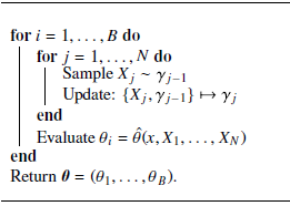
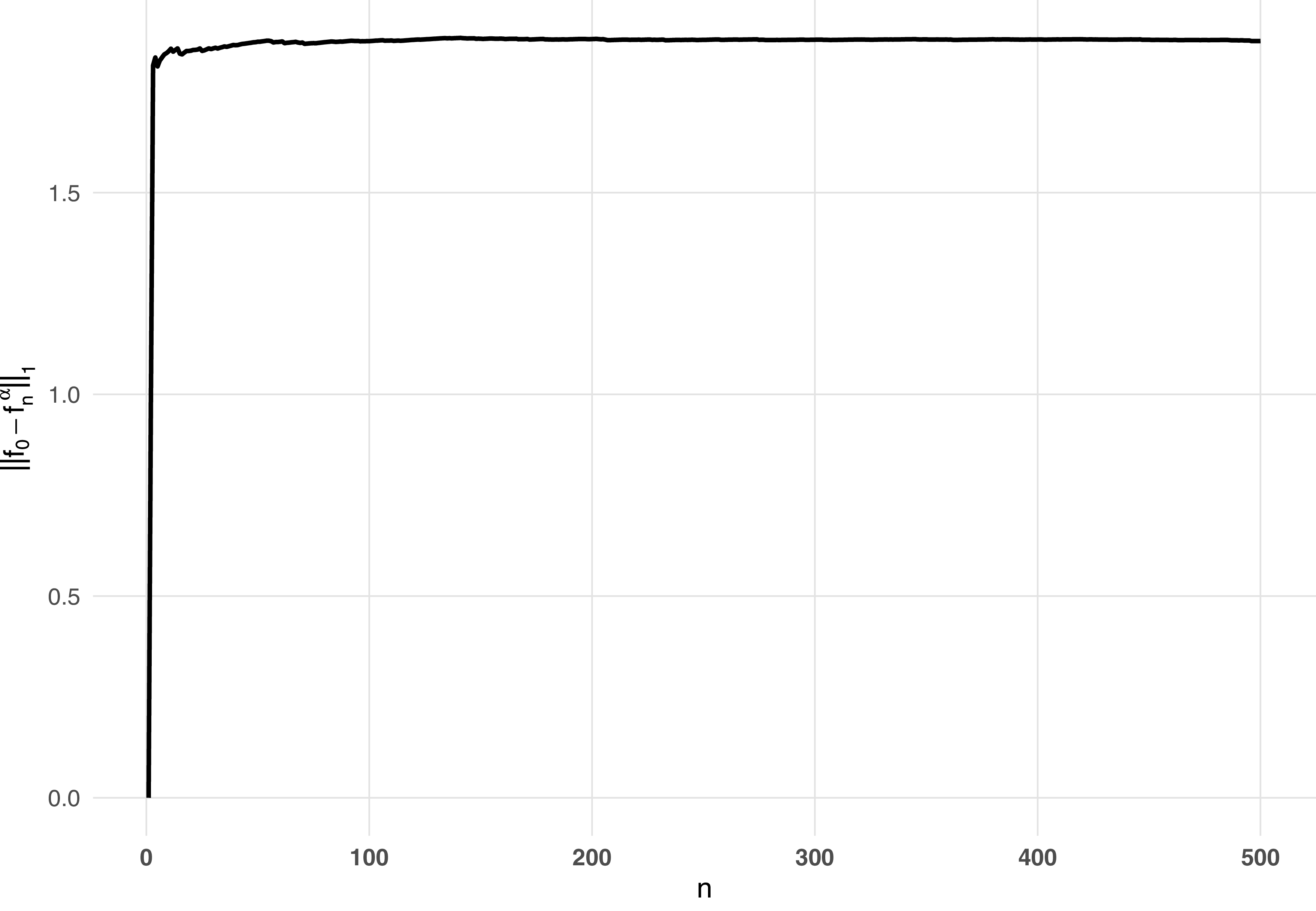
 ||f0−fnα||1
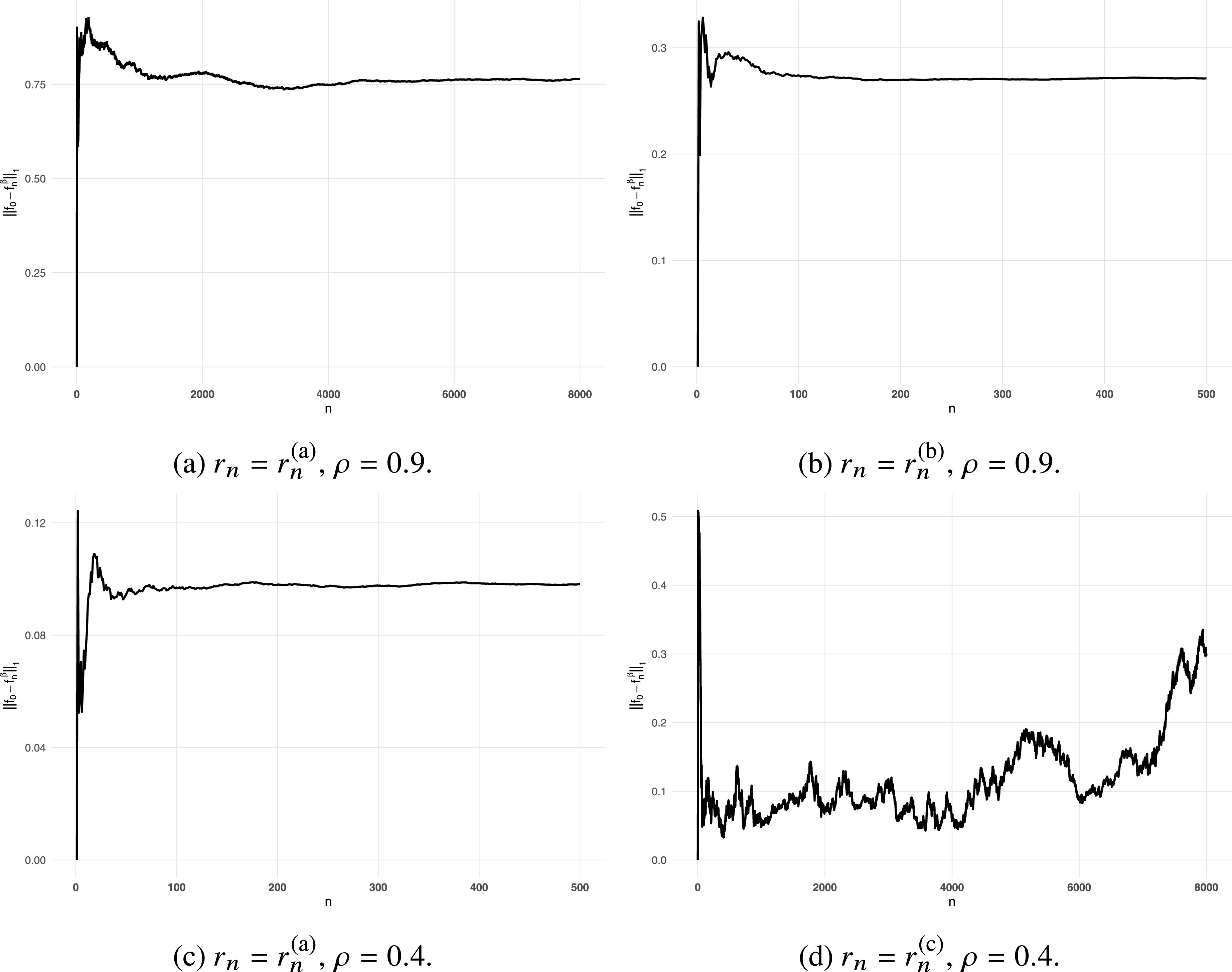
 ||f0−fnβ||1
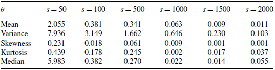
 αn
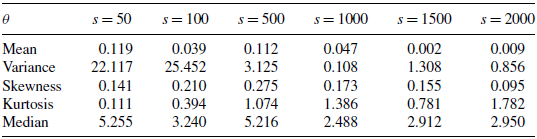
 βn
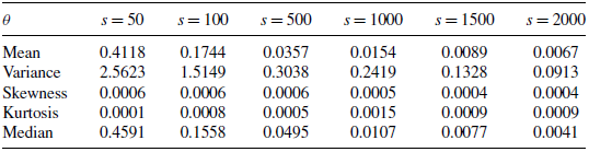
 αn
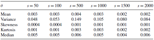
 βn

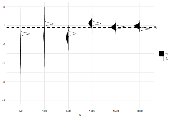
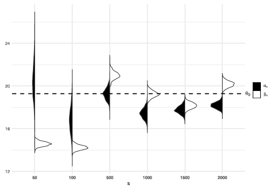
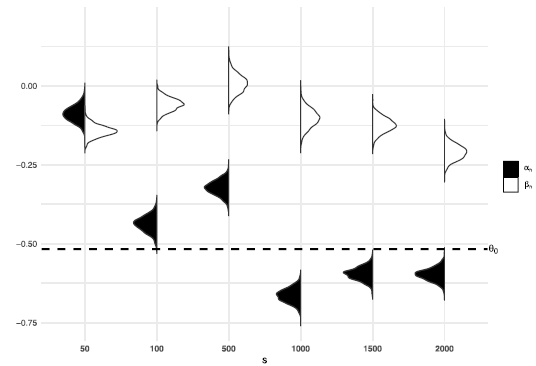
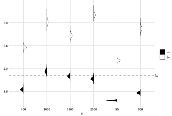
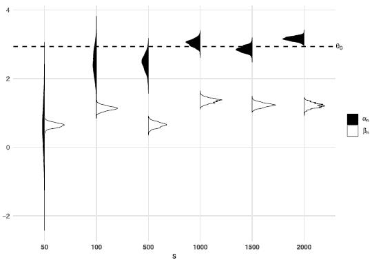

 Open access

