2.1 Preliminaries

First, we recall some decay and smoothing estimates for the linear heat equation.

Lemma 2.1 For any $p,q,r\in \left [1,\infty \right ]$ with $p^{-1}=q^{-1}-r^{-1}$ , any $\varphi \in L^q_{x}$ , and any $k\in \mathbb {N}_0$ , we have

(2.1) $$ \begin{align} \left\|D^{k}_{x} e^{t\Delta}\varphi\right\|_{L^p_x} \lesssim t^{-\frac12\left(\frac{d}{r}+k\right)}\left\|\varphi\right\|_{L^q_{x}} \quad \forall \ t>0. \end{align} $$

In the important special case $p=q, r=\infty , k=0$ , we get

(2.2) $$ \begin{align} \left\|e^{t\Delta}\varphi\right\|_{L^p_{x}} \leq \left\|\varphi\right\|_{L^p_{x}} \quad \forall \ t>0. \end{align} $$

Additionally, we need a result about the function $r(T)$ defined in (1.1).

Lemma 2.2 For any $p\in \mathbb {N}_0$ , there exists a constant $C(p)$ such that

$$ \begin{align*}r(T) \leq C(p) T^{p} \quad \forall \ T\in [0,1]. \end{align*} $$

2.2 Mild solutions and their basic properties

We may use Duhamel’s principle to re-formulate (1.2) in a way that lets us introduce solutions with limited regularity.

Definition 2.1 Let $A, A_0$ , and B be Banach subspaces of $L^{\infty }_{x}$ , with $A \subseteq A_0$ . Suppose we are given an initial datum $\left (T_0(x), Y_0(x)\right )\in A_0 \times B$ . We say that $\left (T(x,t), Y(x,t)\right )\in C^0_t A \times C^0_t B$ is a mild solution of (1.2) if this pair satisfies

(2.3a) $$ \begin{align} T(x,t) &= e^{-\lambda t}e^{t\Delta}T_0 + \int_{0}^{t} e^{-\lambda\left(t-\tau\right)}e^{\left(t-\tau\right)\Delta} Y(x,\tau)r\left(T(x,\tau)\right) \ {\mathrm{d}} \tau \end{align} $$

(2.3b) $$ \begin{align}\ Y(x,t) &= Y_0(x) \exp\left(-\beta\int_0^t r\left(T(x,\sigma)\right) \ {\mathrm{d}} \sigma\right).\quad\qquad\qquad \end{align} $$

Below, the time interval on which a mild solution is valid will be specified when it’s vital to know. Immediately, one sees that mild solutions have some important properties.

1. (1) First, if $Y_0(x)\geq 0$ everywhere then $Y(x,t)\geq 0$ also holds. This makes perfect sense: an initially nonnegative fuel density should never become negative.

2. (2) Second, owing to the smoothing properties of the heat flow $e^{t\Delta }$ , $T(x,t)$ is smooth in x for every $t>0$ . However, $Y(x,t)$ is only as smooth as $Y_0(x)$ .

3. (3) By construction, any mild solution $\left (T,Y\right )$ is continuous in t: in fact, it’s trivial to see that $Y(x,t)$ is also continuously differentiable in t. If we denote the right-hand side of (2.3a) by $\Phi \left [T,Y\right ]$ , then we have

   $$ \begin{align*} \partial_{t}\Phi\left[T,Y\right] = \left(-\lambda+\Delta\right)e^{-\lambda t}e^{t\Delta}T_0 + Y(x,t)r\left(T(x,t)\right) + \int_{0}^{t} \cdots \ {\mathrm{d}} \tau, \end{align*} $$
   where the unimportant particulars in the integral over $\tau $ have been omitted. Each term on the right-hand side of the above expression is continuous in t, so we conclude that $T(x,t)$ is continuously differentiable in t. Thus, in the notation of Definition 2.1, we could just as well define mild solutions as living in $C^1_t A \times C^1_t B$ .

In light of the last two items above, I have almost shown that any mild solution is actually a classical solution to (1.2) (the converse statement is obvious). However, to avoid technicalities about the nature of the convergence of $\left (T(x,t), Y(x,t)\right )\rightarrow \left (T_0(x), Y_0(x)\right )$ as $t\rightarrow 0^{+}$ , I won’t formalize such a statement here: in the sequel, the spatial and temporal regularity of mild solutions turns out to be sufficient to get the estimates I want.

2.3 A priori estimates and existence-uniqueness theory

In this subsection, I prove some basic a priori bounds on mild solutions to (1.2) with $\lambda>0$ . These bounds are then used to help construct global-in-time mild solutions of (1.2). We start with the easiest bound possible.

Proposition 2.3 For any $p\in [1,\infty ]$ , if $(T,Y)$ is a mild solution of (1.2), then

(2.4) $$ \begin{align} \sup_{t>0}\left\|Y(x,t)\right\|_{L^p_{x}} \leq \left\|Y_0(x)\right\|_{L^p_{x}} \end{align} $$

provided the right-hand side is finite.

According to Mandel et al. [Reference Mandel, Bennethum, Beezley, Coen, Douglas, Kim and Vodacek13, Section 4.1], $Y(x,t)$ is expected to settle to a small but nonzero steady value for $t\gg 1$ . I therefore do not think one can prove a variant of the above result that includes a time-dependent decay factor going to $0$ as $t\rightarrow \infty $ on the right-hand side.

Proposition 2.4 Suppose $\lambda>0$ . If we are given an initial datum $(T_0, Y_0)\in L^{\infty }_{x}\times L^{\infty }_{x}$ and a corresponding mild solution $(T,Y)\in C^{0}_{t}L^{\infty }_{x}\times C^{0}_{t}L^{\infty }_{x}$ of (1.2), then

(2.5) $$ \begin{align} \left\|T(x,t)\right\|_{L^{\infty}_{x}} \leq e^{-\lambda t}\left\|T_0(x)\right\|_{L^{\infty}_{x}} + \lambda^{-1}\left\|Y_0(x)\right\|_{L^{\infty}_{x}}. \end{align} $$

Proof Using Lemma 2.1 and $\left |r(T)\right |\leq 1$ , we have

$$ \begin{align*} \left\|T\right\|_{L^{\infty}_{x}} &\leq e^{-\lambda t} \left\|T_0\right\|_{L^{\infty}_{x}} + \sup_{t>0}\left\|Y r\left(T\right)\right\|_{L^\infty_x}\int_0^t e^{-\lambda \left(t-\tau\right)} \ {\mathrm{d}} \tau \\ &\leq e^{-\lambda t} \left\|T_0\right\|_{L^{\infty}_{x}} + \lambda^{-1}\left(1-e^{-\lambda t}\right)\left\|Y_0\right\|_{L^\infty_x}.\\[-34pt] \end{align*} $$

Proposition 2.5 Suppose $\lambda>0$ . If we are given an initial datum $(T_0, Y_0)\in \left (L^{2}_{x}\cap L^{\infty }_{x}\right )\times L^{\infty }_{x}$ and a corresponding mild solution $(T,Y)\in C^{0}_{t}\left (L^{2}_{x}\cap L^{\infty }_{x}\right )\times C^{0}_{t}L^{\infty }_{x}$ of (1.2), then

(2.6) $$ \begin{align} \left\|T\right\|_{L^2_{x}}^2 \lesssim \min\left\{\left\|T_0\right\|_{L^2_{x}}^2 + C\left(\left\|T_0\right\|_{L^{\infty}_{x}}, \left\|Y_0\right\|_{ L^{\infty}_{x}}, \lambda, \beta\right)\left\|Y_0- Y\right\|_{L^1_{x}}, \ \left\|T_0\right\|_{L^2_{x}}^2 e^{\left\|Y_0\right\|_{L^{\infty}_{x}}t}\right\}. \end{align} $$

In particular, if $(T_0, Y_0)\in \left (L^{2}_{x}\cap L^{\infty }_{x}\right )\times \left (L^{1}_{x}\cap L^{\infty }_{x}\right )$ then

(2.7) $$ \begin{align} \sup_{t>0}\left\|T(x,t)\right\|_{L^2_{x}} \leq C\left(\left\|T_0\right\|_{L^2_{x}\cap L^{\infty}_{x}}, \left\|Y_0\right\|_{L^1_{x}\cap L^{\infty}_{x}}, \lambda, \beta\right). \end{align} $$

Proof Recall that $T(x,t)$ is smooth in x and continuously differentiable in t, so we can write $T_{t} = \left (\Delta -\lambda \right ) T + Yr\left (T\right )$ for $t>0$ . We then use a standard energy argument:

(2.8) $$ \begin{align} \frac{{\mathrm{d}}}{{\mathrm{d}} t}\frac12 \left\|T\right\|_{L^2_{x}}^2 &= - \left\|T\right\|^2_{\dot{H}^1_{x}} -\frac{\lambda}{2}\left\|T\right\|_{L^2_x}^2+ \int T(x,t) \ Y(x,t) \ r\left(T(x,t)\right) \ {\mathrm{d}} x \nonumber \\ &\leq \int T(x,t) \ Y(x,t) \ r\left(T(x,t)\right) \ {\mathrm{d}} x \\ &= \beta^{-1} \int T(x,t) \ \left(-Y_{t}(x,t)\right) \ {\mathrm{d}} x \nonumber \\ &\leq \beta^{-1}\sup_{t>0}\left\|T(x,t)\right\|_{L^{\infty}_{x}}\int \left(-Y_{t}(x,t)\right) \ {\mathrm{d}} x. \nonumber \end{align} $$

Integrating both sides of the above over $[0,t]$ and using Proposition 2.4 gives

$$ \begin{align*} \left\|T(x,t)\right\|_{L^2_{x}}^2 \lesssim \left\|T_0(x)\right\|_{L^2_{x}}^2 + C\left(\left\|T_0\right\|_{L^{\infty}_{x}}, \left\|Y_0\right\|_{ L^{\infty}_{x}}, \lambda, \beta\right)\int_0^t\int \left(-Y_{\tau}(x,\tau)\right) \ {\mathrm{d}} x \ {\mathrm{d}} \tau. \end{align*} $$

Then, we use the Fubini–Tonelli theorem (valid since $-Y_{\tau }$ is non-negative and measurable) and the fundamental theorem of calculus to obtain one part of (2.6). The special case (2.7) follows since $Y_0(x) - Y(x,t) \leq Y_0(x)$ . For the other part of (2.6), we instead use $Tr(T)\lesssim T^2$ in (2.8), place Y in $L^{\infty }_{x}$ , and conclude with an application of Grönwall’s inequality.

Next, I demonstrate how these a priori estimates may be applied to obtain global-in-time mild solutions to (1.2).

Proof Local-in-time existence and uniqueness follows from a routine fixed-point argument. Let $\Phi \left [T,Y\right ]$ denote the right-hand side of (2.3a) and let $\Psi \left [T,Y\right ]$ denote the right-hand side of (2.3b) (note that $T_0, Y_0$ are fixed). We want to show that there exist $R>0$ and $t^{*}\in (0,1)$ such that $(T,Y)\mapsto \left (\Phi \left [T,Y\right ], \Psi \left [T,Y\right ]\right )$ is a contraction mapping on the open ball $B(0,R)\subseteq C^0_t L^{\infty }_{x}\times C^0_t L^{\infty }_{x}$ , where time takes values in $[0,t^{*}]$ . Arguments similar to those applied in Propositions 2.3 and 2.4 show that this mapping takes $B(0,R)$ to itself if

(2.9a) $$ \begin{align} \left\|T_0\right\|_{L^{\infty}_x} + \left\|Y_0\right\|_{L^{\infty}_x} + t^{*}R \leq R. \end{align} $$

Analogous techniques, when combined with the mean value theorem in two variables, show that for any $\left (T_1, Y_1\right ), \left (T_2, Y_2\right )\in B(0,R)$ we have the Lipschitz-type estimates

$$ \begin{align*} \left\|\Phi\left[T_1,Y_1\right]- \Phi\left[T_2,Y_2\right]\right\|_{C^0_t L^{\infty}_{x}} &\leq CRt^{*}\left\|\left(T_1, Y_1\right) -\left(T_2, Y_2\right)\right\|_{C^0_t L^{\infty}_{x}\times C^0_t L^{\infty}_{x}}, \\ \left\|\Psi\left[T_1,Y_1\right]- \Psi\left[T_2,Y_2\right]\right\|_{C^0_t L^{\infty}_{x}} &\leq \beta R t^{*}\left\|\left(T_1, Y_1\right) -\left(T_2, Y_2\right)\right\|_{C^0_t L^{\infty}_{x}\times C^0_t L^{\infty}_{x}}, \end{align*} $$

where C is independent of $R, t^{*}$ . Accordingly, $(T,Y)\mapsto \left (\Phi \left [T,Y\right ], \Psi \left [T,Y\right ]\right )$ certainly defines a contraction on $B(0,R)$ if

(2.9b) $$ \begin{align} t^{*}\leq \frac12 \min\left\{1, \left(C+\beta\right)^{-1}R^{-1}\right\}. \end{align} $$

Choosing $R=4\left (\left \|T_0\right \|_{L^\infty _{x}} + \left \|Y_0\right \|_{L^\infty _{x}}\right )$ and letting $t^{*}$ saturate (2.9b), we find that (2.9a) is also satisfied. Applying Banach’s contraction mapping theorem, the proof of existence and uniqueness of a mild solution within $B(0,R)$ is complete. Unconditional uniqueness then follows from the bootstrap principle (see for instance [Reference Tao19, pp. 131–132 for further details).

If $\lambda>0$ then Propositions 2.3 and 2.4 allow us to extend this local solution to a global one. With this solution in hand, we apply Proposition 2.5 to conclude.

Consequently, solutions to (1.2) do not exhibit thermal blow-up when $\lambda>0$ . In the case $\lambda =0$ the techniques from Proposition 2.4 would yield

$$ \begin{align*} \left\|T(x,t)\right\|_{L^{\infty}_{x}} \leq\left\|T_0(x)\right\|_{L^{\infty}_{x}} + t\left\|Y_0(x)\right\|_{L^{\infty}_{x}}. \end{align*} $$

While this does not give a nice uniform-in-time bound, it at least says that thermal blow-up does not occur in finite time irrespective of $\lambda $ .

For the sake of completeness, I mention that we can obtain coarse estimates on $\nabla T$ without too much trouble.

Proposition 2.7 Pick $p,q,\ell \in \left [1,\infty \right ]$ with $p^{-1}=q^{-1}-\ell ^{-1}$ and $\ell>d$ . If $(T_0, Y_0)\in \left (L^{p}_{x}\cap L^{\infty }_{x}\right )\times \left (L^{q}_{x}\cap L^{\infty }_{x}\right )$ then the corresponding mild solution $(T,Y)$ of (1.2) satisfies

(2.10) $$ \begin{align} \left\|\nabla T(x,t)\right\|_{L^p_{x}} \lesssim t^{-\frac12} \left\|T_0(x)\right\|_{L^p_x} + t^{\frac12\left(1-\frac{d}{\ell}\right)}\left\|Y_0\right\|_{L^q_x} \quad \forall \ t>0. \end{align} $$

In particular,

(2.11) $$ \begin{align} \left\|\nabla T(x,t)\right\|_{L^\infty_{x}} \lesssim t^{-\frac12} \left\|T_0(x)\right\|_{L^\infty_x} + t^{\frac12}\left\|Y_0\right\|_{L^\infty_x} \quad \forall \ t>0. \end{align} $$

Proof Using (2.1), (2.4), and $|r(T)|\leq 1$ , we have

$$ \begin{align*} \left\|\nabla T(x,t)\right\|_{L^{p}_{x}} &\lesssim t^{-\frac{1}{2}}\left\|T_0\right\|_{L^p_{x}} + \left\|Y_0\right\|_{L^q_x}\int_0^t \left(t-\tau\right)^{-\frac{1}{2}\left(\frac{d}{\ell}+1\right)} \ {\mathrm{d}} \tau \end{align*} $$

and we’re all done upon computing the integral.

This re-affirms that solutions of (1.2) do not develop sharp edges in finite time (see the discussion in the second point under Definition 2.1). I expect that one can get rid of the temporally growing term in (2.10) using more sophisticated techniques.

2.4 Decay of small-data solutions

Next I show that, if the initial temperature $T_0$ is sufficiently small, then $\lim _{t\rightarrow \infty }|T(x,t)|=0$ uniformly. This confirms that (1.2) has a nonzero auto-ignition temperature up to some mild assumptions on $T_0$ . From our work in the last section, we know that $\lambda =0$ gives the worst $L^{\infty }_x$ temperature bounds possible, so in this section we choose $\lambda =0$ : if we can establish decay with $\lambda =0$ then it is even simpler to establish decay with $\lambda>0$ . While this means we don’t have access to the existence-uniqueness results from the previous section, we can still build a temporally-decaying global solution using the assumption of small initial data and the bootstrap principle. This strategy for establishing time decay is well-known in the theory of dispersive PDEs, see for instance [Reference Morgan16].

Throughout this section, we suppose that ${\epsilon }_0\in (0,1)$ is a small parameter (to be constrained later) and

(2.12) $$ \begin{align} \left\|T_0\right\|_{L^1_x\cap L^{\infty}_x} < {\epsilon}_0 \quad \text{and} \quad \left\|Y_0\right\|_{L^{\infty}_x} < \infty. \end{align} $$

The requirement that $T_0$ is small in $L^1_x$ expresses that the initial temperature is approximately localized in space. Strictly speaking, smallness in any $L^q_{x}$ -norm with $q<\infty $ would also capture localization, but the choice $q=1$ is a minor technical one giving us access to a good decay estimate. Now, given $t_{*}\in (0,\infty ]$ and a sufficiently nice function $T(x,t)$ defined for $t\in [0,t_{*}]$ , we set

$$ \begin{align*} \left\|T(x,t)\right\|_{X_{t_{*}}} \doteq \sup_{t\in [0,t_{*}]}\left[ \left(1+t\right)^{\frac{d}{2}}\left\|T(x,t)\right\|_{L^{\infty}_{x}}+ \left\|T(x,t)\right\|_{L^1_x}\right]. \end{align*} $$

This norm naturally gives rise to a Banach space $X_{t_{*}}$ defined by

$$ \begin{align*} X_{t_{*}} \doteq \left\{T\colon [0,t_{*}] \rightarrow L^1_x \cap L^\infty_{x}\ \text{continuous}\ \bigg| \ \left\|T(x,t)\right\|_{X_{t_{*}}} < \infty\right\}. \end{align*} $$

The first order of business is to prove a new a priori estimate for solutions that are small in $X_{t_*}$ .

Proposition 2.8 Take ${\epsilon }_1 \in \left [{\epsilon }_0, 1\right )$ . Assume that (2.12) holds and that there is a corresponding mild solution $\left (T,Y\right )\in X_{t_{*}}\times C^0_t L^{\infty }_{x}$ to (1.2) valid on $[0,t_{*}]$ . Further, assume that $\left \|T\right \|_{X_{t_{*}}} \leq {\epsilon }_1$ . Then, there exists an absolute constant $C>0$ such that

(2.13) $$ \begin{align} \left\|T(x,t)\right\|_{X_{t_{*}}} \leq 2^{1+d/2}{\epsilon}_0 + C\left\|Y_0\right\|_{L^\infty_x} {\epsilon}_1^{11}. \end{align} $$

Proof Let’s look at the $L^{\infty }_{x}$ part of the $X_{t_{*}}$ norm first. Together with the hypothesis of our claim, Lemma 2.2 (with $p=11$ ) implies

$$ \begin{align*} \left\|r(T)\right\|_{L^\infty_x} &\leq C\left\|T\right\|_{L^{\infty}_x}^{11} \leq C \left({\epsilon}_1 \left(1+t\right)^{-\frac{d}{2}}\right)^{11} \leq C{\epsilon}_1^{11}\left(1+t\right)^{-\frac{11}{2}d} \end{align*} $$

and

$$ \begin{align*} \left\|r(T)\right\|_{L^1_x}\leq C\left\|T^{10}\right\|_{L^{\infty}_{x}}\left\|T\right\|_{L^1_{x}} \leq C\left[{\epsilon}_1\left(1+t\right)^{-\frac{d}{2}}\right]^{10}{\epsilon}_1 \leq C{\epsilon}_1^{11}\left(1+t\right)^{-5d}. \end{align*} $$

There is nothing special about the choice $p=11$ : any large enough natural number will do, and the rapid vanishing of $r(T)$ at $T=0$ guarantees we can pick such a large p. We first focus on the $t>1$ case. Combining the estimates on $r(T)$ with the definition of a mild solution, (2.1), the easy bound $2t \geq 1+t$ for $t>1$ , (2.2), and (2.12), we have

$$ \begin{align*} \left\|T(x,t)\right\|_{L^\infty_x} &\leq 2^{d/2}\left(1+t\right)^{-\frac{d}{2}} {\epsilon}_0 + \int_0^t \left\|e^{\left(t-\tau\right)\Delta} Y(x,\tau)r\left(T(x,\tau)\right)\right\|_{L^\infty_x} \ {\mathrm{d}} \tau \\ &\leq 2^{d/2}\left(1+t\right)^{-\frac{d}{2}} {\epsilon}_0 + \int_0^{t/2} \left(t-\tau\right)^{-\frac{d}{2}} \left\|Y(x,\tau) \ r\left(T(x,\tau)\right)\right\|_{L^1_{x}} \ {\mathrm{d}} \tau \\ &\phantom{\leq} + \int_{t/2}^t \left\|Y(x,\tau) \ r\left(T(x,\tau)\right)\right\|_{L^\infty_{x}} \ {\mathrm{d}} \tau \\ &\leq 2^{d/2}\left(1+t\right)^{-\frac{d}{2}} {\epsilon}_0 + C\left\|Y_0\right\|_{L^\infty_{x}} {\epsilon}_1^{11} \left[\int_0^{t/2} \left(1+t-\tau\right)^{-\frac{d}{2}} \left(1+\tau\right)^{-5d} \ {\mathrm{d}} \tau \right. \\ &\phantom{\leq} \left. +\int_{t/2}^t \left(1+\tau\right)^{-\frac{11}{2}d} \right] \\ &\leq 2^{d/2}\left(1+t\right)^{-\frac{d}{2}}\left[{\epsilon}_0 + C\left\|Y_0\right\|_{L^\infty_x} {\epsilon}_1^{11}\right]. \end{align*} $$

For $t\leq 1$ we may apply an almost identical approach, but we don’t split the Duhamel term and we only use (2.2). This takes care of the $L^\infty _x$ piece. The $L^1_{x}$ estimate is obtained by a similar but even easier argument using (2.2) to control $\left \|e^{\left (t-\tau \right )\Delta }Yr\left (T\right )\right \|_{L^1_x}$ .

Theorem 2.9 There exists ${\epsilon }_0 ={\epsilon }_0\left (\left \|Y_0\right \|_{L^\infty _x},d\right )\in (0,1)$ such that, under the hypothesis (2.12), (1.2) admits a unique global-in-time mild solution $\left (T,Y\right )\in X_{\infty }\times C^0_t L^{\infty }_x$ obeying the decay estimate

(2.14) $$ \begin{align} \left\|T(x,t)\right\|_{L^{\infty}_{x}} \lesssim_d {\epsilon}_0 \left(1+t\right)^{-\frac{d}{2}}. \end{align} $$

In particular, $\lim _{t\rightarrow \infty }|T(x,t)| = 0$ uniformly in x.

Proof Using fixed-point iteration as in Corollary 2.6, one finds a $t_{*}>0$ such that (1.2) has a unique local-in-time mild solution valid on $[0,t_*]$ with $T(x,t)\in X_{t_{*}}$ . Further, the map $\tau \mapsto \left \|T\right \|_{X_\tau }$ is easily shown to be continuous for $\tau \in [0,t_*]$ . Accordingly, for sufficiently small $t_{*}$ and $\alpha>2+\frac {d}{2}$ we know $\left \|T\right \|_{X_{t_{*}}}\leq 2^{\alpha }{\epsilon }_0$ . Now, apply Proposition 2.8 with ${\epsilon }_1 = 2^{\alpha }{\epsilon }_0$ to discover

$$ \begin{align*} \left\|T\right\|_{X_{t_{*}}} \leq 2^{1+d/2}{\epsilon}_0 \left(1 + 2^{11\alpha - 1 -\frac{d}{2}}C \left\|Y_0\right\|_{L^\infty_x} {\epsilon}_0^{10}\right). \end{align*} $$

By choosing ${\epsilon }_0 < \frac 12\left (2^{11\alpha - 1 -\frac {d}{2}}C\left \|Y_0\right \|_{L^\infty _x}\right )^{-\frac {1}{10}}$ , the above becomes $\left \|T\right \|_{X_{t_{*}}}\leq 2^{2+d/2}{\epsilon }_0$ . Since $\alpha>2+\frac {d}{2}$ , this bound is nontrivial. The bootstrap principle (see for example [Reference Tao19]) allows us to iterate this argument, giving a global solution satisfying $\left \|T\right \|_{X_{\infty }}\lesssim _d {\epsilon }_0$ .

The ${\epsilon }_0$ from Theorem 2.9 should be regarded as a lower bound on the auto-ignition temperature for the model (1.2), but my methods cannot determine how sharp this bound is. However, a simple numerical experiment shows that much more work is needed to obtain a precise bound on the auto-ignition temperature. Fix $d=1$ . Using a symbolic computation software like WolframAlpha, one can verify that the constant $C(p)$ from Lemma 2.2 with $p=11$ is on the order of $10^6$ (simply ask the software to find the maximum of $z^{-11}r(z)$ ). Consequently, a bit of arithmetic and the physically meaningful bound $\left \|Y_0\right \|_{L^\infty _x}\leq 1$ show that ${\epsilon }_0$ is on the order of about $10^{-2}$ . Figure 1 displays a numerical simulation of (1.2) with $\beta =1, \lambda =0$ , and initial state

(2.15a) $$ \begin{align} T_0(x) &= \exp\left(-\left(\frac{x}{0.03}\right)^2\right) \end{align} $$

(2.15b) $$ \begin{align} \qquad\, Y_0(x) &= \begin{cases} 1 \quad &x\in [-0.75, 0.75] \\ 0 \quad &\text{else} \end{cases} \end{align} $$

Figure 1

Evolution of the initial state (2.15) with $\beta =1, \lambda =0$ . Note the rapid decay in time despite the initial amplitude being much larger than ${\epsilon }_0$ .

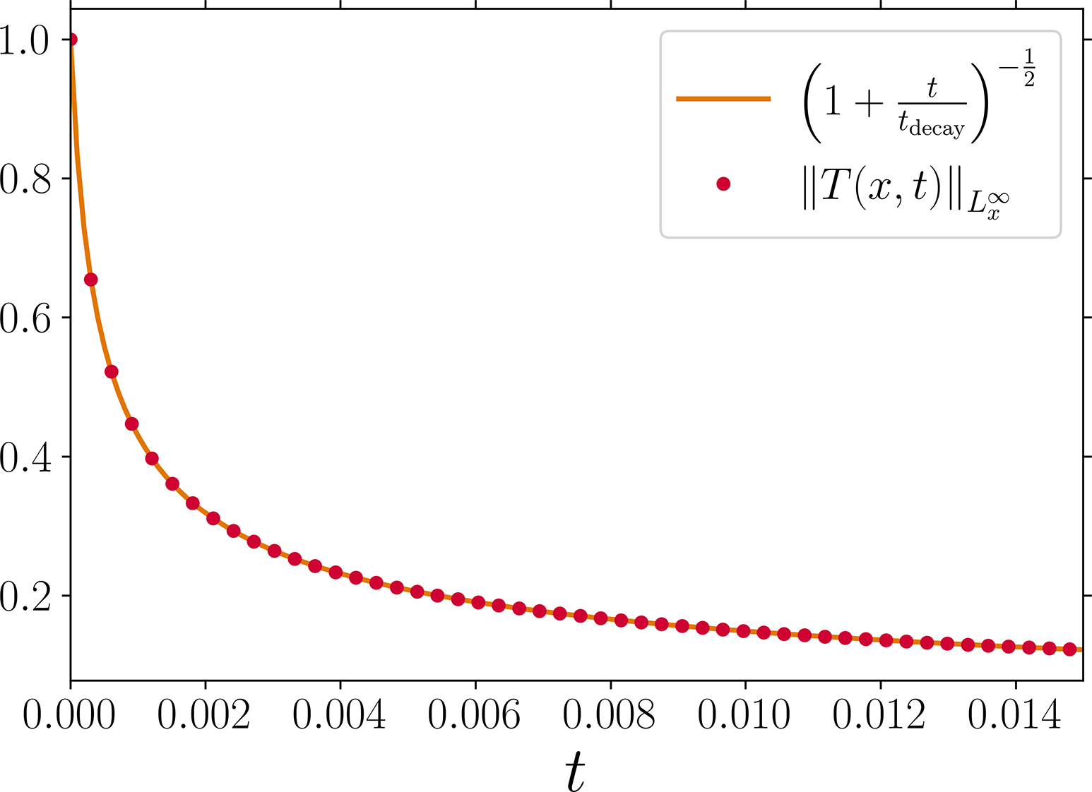
generated using a Chebyshev differentiation matrix in space [Reference Trefethen21], exponential Euler integration in time for the temperature [Reference Hochbruck and Ostermann9], and regular Euler integration in time for the mass ratio. Even though this initial state has an amplitude $\left \|T_0(x)\right \|_{L^\infty _x}$ that is about one hundred times larger than ${\epsilon }_0$ , it still exhibits rapid decay: by $t=0.015$ , $\left \|T(x,t)\right \|_{L^{\infty }_x}$ has already dropped to approximately $10\%$ of its initial value. Accordingly, the ${\epsilon }_0$ obtained in Theorem 2.9 is far too small to be a sharp lower bound on the auto-ignition temperature. Determining a sharp estimate for the auto-ignition temperature, whether by numerical or analytical means, would be an excellent topic for future investigations. Finally, a curve of the form $ t\mapsto \left (1+t/t_{\mathrm {decay}}\right )^{-\frac 12} $ (where $t_{\mathrm {decay}}$ is a decay timescale) can be fit to the numerically-determined amplitude $t\mapsto \left \|T(x,t)\right \|_{L^{\infty }_x}$ using nonlinear least squares; see Figure 2. The similarity between this fit function and the right-hand side of (2.14) suggests that a variant of (2.14) may still hold for initial data near the actual auto-ignition temperature, rather than just for data that is smaller than ${\epsilon }_0$ .

Figure 2

Empirical fit for $\left \|T(x,t)\right \|_{L^{\infty }_x}$ inspired by (2.14). The value of the decay timescale is $t_{\mathrm {decay}}=2.267\times 10^{-4}$ .