
 JGeo,SmallReg(f,s,χ)
 JGeo,DualBig(f,s,χ)





1. Introduction
1.1 The Burgess bound for
 $\mathrm{GL}(2)\times\mathrm{GL}(1)$
over number fields

Let F be a number field. Let
 $\pi$
be a unitary generic automorphic representation of
 $\mathrm{GL}(2)/F$
. In this paper we consider the subconvexity problem for character twists over a number field (ScP(
 $\pi\otimes\chi$
)): finding a constant
 $\delta\in (0,1/2],$
such that
 \begin{equation}L(1/2,\pi\times\chi)\ll_{\pi,F,\varepsilon} C(\chi)^{\frac{1}{2}-\delta+\varepsilon}\end{equation}
holds for all unitary Hecke characters
 $\chi$
over F, where the implied constant relies on
 $\pi,$
F, and
 $\varepsilon.$
Here,
 $C(\chi)$
is the analytic conductor of
 $\chi$
(see § 2.1.1). Note that (1.1) involves the bound of
 $L(s,\pi\times\chi)$
on the critical line
 ${\rm Re}(s)=1/2$
as
 $L(1/2+it,\pi\times\chi)=L(1/2,\pi\times\chi|\cdot|^{it}).$
Moreover, if
 $\pi=\mathbf{1}\boxplus\mathbf{1}$
is the Eisenstein series induced from the trivial character, then
 $L(1/2,\pi\times\chi)=L(1/2,\chi)^2,$
and thus (1.1) becomes the classical subconvexity problem for Hecke L-functions.
The above ScP(
 $\pi\otimes\chi$
) is the pioneering study of the automorphic subconvexity problem in a systematic manner and has been extensively investigated over the years: see, e.g., [Reference BurgessBur63, Reference Heath-BrownHea78, Reference Heath-BrownHea80, Reference Conrey and IwaniecCI00, Reference Duke, Friedlander and IwaniecDFI02, Reference MilićevićMil16, Reference YoungYou17, Reference WuWu19, Reference Petrow and YoungPY23, Reference Petrow and YoungPY20] for the case when
 $\pi$
is an Eisenstein series, and see [Reference Duke, Friedlander and IwaniecDFI93, Reference BykovskiByk96, Reference Cogdell, Piatetski-Shapiro and SarnakCPS01, Reference Blomer, Harcos and MichelBHM07, Reference Blomer and HarcosBH08, Reference VenkateshVen10, Reference Michel and VenkateshMV10, Reference Blomer and HarcosBH10, Reference Blomer and HarcosBH14, Reference WuWu14, Reference MagaMag17, Reference MunshiMun18, Reference NelsonNel19, Reference Aggarwal, Holowinsky, Lin and SunAHL+20, Reference Fan and SunFS22] for the case when
 $\pi$
is cuspidal. The subconvex bound of type (1.1) is a versatile tool with numerous applications in arithmetic geometry, as highlighted in Remark 1.4 below, which provides several illustrative examples. One notable instance involves the work of [Reference Cogdell, Piatetski-Shapiro and SarnakCPS01], where the authors were the first to investigate ScP(
 $\pi\otimes\chi$
) in the case of F being a number field other than
 $\mathbb{Q}$
in connection with Hilbert’s eleventh problem. This groundbreaking investigation paved the way for further developments in the analytic theory of L-functions, leading to the emergence of the ScP(
 $\pi\otimes\chi$
) problem over number fields as a significant area of study.
The Lindelöf hypothesis predicts that (1.1) holds with
 $\delta=1/2$
. When
 $F=\mathbb{Q}$
, the tightest known bound for (1.1) is
 $\delta=1/8$
(see, e.g., [Reference Blomer and HarcosBH08]). In the special case that
 $\pi\otimes\chi$
has a trivial central character, Petrow and Young (see [Reference Petrow and YoungPY20, Reference Petrow and YoungPY23]) have proved that (1.1) holds for
 $\delta = 1/6$
. In the more general situation where
 $F\neq\mathbb{Q}$
, the best-known result is
 $\delta=(1-2\vartheta)/8$
(see [Reference WuWu14, Reference WuWu19]), where
 $0\leqslant \vartheta\lt1/2$
is any exponent towards the Ramanujan–Petersson conjecture (RPC) for unitary cuspidal representations of
 $\mathrm{GL}(2)/F$
. Currently, the strongest known value is
 $\vartheta=7/64$
(see [Reference Kim and SarnakKS03, Reference Blomer and BrumleyBB11]). Hence, the most favorable unconditional bound in the general case is
 $\delta=1/8-7/256$
. Nevertheless, under the RPC, i.e.,
 $\vartheta = 0$
, one obtains the bound
 $\delta = 1/8$
.
This is conventionally referred to as the Burgess bound, since when
 $F = \mathbb{Q}$
,
 $\pi = \mathbf{1} \boxplus \mathbf{1}$
,
 $\chi$
is a primitive Dirichlet character modulo q, and
 $\delta = 1/8$
, then (1.1) reduces to the classical bound
 $L(1/2, \chi) \ll q^{3/16 + \varepsilon}$
obtained by Burgess [Reference BurgessBur63]. For general
 $\mathrm{GL}(2)$
L-functions, the Burgess bound represents a natural barrier that may require new ideas to overcome.
The first achievement of this paper confirms (1.1) with
 $\delta=1/8$
for any unitary generic
 $\pi$
and unitary characters
 $\chi$
over F, obtaining the Burgess bound without assuming RPC.
Theorem 1.1.
Let
 $\pi$
be a unitary generic automorphic representation of
 $\mathrm{GL}(2)/F$
, and let
 $\chi$
be a unitary Hecke character over F. Then
 \begin{equation}L(1/2,\pi\times\chi)\ll_{\pi,F,\varepsilon}C(\chi)^{\frac{1}{2}-\frac{1}{8}+\varepsilon}.\end{equation}
Corollary 1.2.
Let
 $\chi$
be a unitary Hecke character over F. Then
 \begin{equation}L(1/2,\chi)\ll_{F,\varepsilon}C(\chi)^{\frac{1}{4}-\frac{1}{16}+\varepsilon}.\end{equation}
Let
 $\pi$
be a unitary cuspidal representation of
 $\mathrm{GL}(2)/F.$
Then
 \begin{equation}L(1/2,\pi\times\chi)\ll_{\pi,F,\varepsilon}C(\chi)^{\frac{1}{2}-\frac{1}{8}+\varepsilon}.\end{equation}
Remark 1.3. The estimate (1.3) improves [Reference WuWu19], and (1.4) improves [Reference BykovskiByk96, Reference Blomer, Harcos and MichelBHM07, Reference Blomer and HarcosBH08, Reference Blomer and HarcosBH10, Reference Blomer and HarcosBH14, Reference WuWu14, Reference MagaMag17].
Remark 1.4. By Waldspurger’s formula in [Reference WaldspurgerWal85], Theorem 1.1 has direct implications in:
-
– bounding Fourier coefficients of half-integral-weight Hilbert modular forms (particularly including those with nontrivial central characters);
-
– computing the asymptotic of representation numbers of quadratic forms with power saving error terms (see [Reference Cogdell, Piatetski-Shapiro and SarnakCPS01, Reference CogdellCog03, Reference Blomer and HarcosBH10]); and
-
– effective equidistribution of CM points and certain subvarieties on the Hilbert modular surface (see, e.g., [Reference DukeDuk88], [Reference ZhangZha05, Theorem 3.2], [Reference CohenCoh05, Theorem 1.2], and [Reference VenkateshVen10, § 1.1]).

1.2 Explicit hybrid bounds
Theorem 1.1 follows readily from the following refined hybrid subconvex bound for twisted L-functions.
Theorem 1.6.
Let F be a number field with ring of adeles
 $\mathbb{A}_F$
. Let
 $\pi=\otimes_{v}\pi_v$
be a unitary generic automorphic representation of
 $\mathrm{GL}(2)/F$
with central character
 $\omega.$
Let
 $\chi=\otimes_{v}\chi_v$
be a unitary Hecke character of
 $\mathbb{A}_F^{\times}/F^{\times}$
. For an Archimedean place v, let
 $\iota_v\in\{0,1/2\}$
be the constant defined by (2.2), determined by the structure of
 $\pi_v\otimes\chi_v$
. Then
 \begin{align*}L(1/2,\pi\times\chi)&\ll_{F,\varepsilon} [C_{{\rm fin}}(\pi),C_{{\rm fin}}(\omega)C_{{\rm fin}}(\chi)]^{\frac{1}{4}+\varepsilon}C_{{\rm fin}}(\chi)^{\frac{1}{8}+\varepsilon}\prod_{v\mid\infty}C_{v}(\pi\otimes\chi)^{\frac{3}{16}+\frac{3\iota_v}{8}+\varepsilon}\\&\quad +C_{{\rm fin}}(\pi)^{\frac{1}{2}+\varepsilon}C_{{\rm fin}}(\chi)^{\frac{1}{4}+\varepsilon}C_{\infty}(\pi)^{\frac{1}{4}+\varepsilon}\prod_{v\mid\infty}C_{v}(\pi\otimes\chi)^{\frac{1}{8}+\frac{\iota_v}{4}+\varepsilon}.\end{align*}
Here, for a representation
 $\sigma=\otimes_{v}\sigma_v$
of
 $\mathrm{GL}(1)$
or
 $\mathrm{GL}(2)/F,$
 $C_v(\sigma)$
is the associated local conductor (see § 2.1.1),
 $C_{\infty}(\sigma)=\prod_{v\mid\infty}C_v(\sigma),$
and
 $C_{{\rm fin}}(\sigma)=\prod_{v\lt\infty}C_v(\sigma).$
Remark 1.7. We have
 $\iota_v = 0$
for
 $v\mid\infty$
if the spectral parameters of
 $\pi_v\otimes\chi_v$
are comparable; otherwise,
 $\iota_v = 1/2$
, in which case
 $C_v(\chi)\ll C_v(\pi)$
. Thus, when
 $\pi_{\infty}$
is fixed, we have
 $\iota_v=0$
for all
 $v\mid\infty$
; this is the scenario considered in Theorem 1.1.
Remark 1.8. Theorem 1.6 refines and extends the bounds established in several previous works. In the case over
 $\mathbb{Q}$
, it strengthens the results of [Reference Blomer, Harcos and MichelBHM07, Reference Blomer and HarcosBH08, Reference Blomer and HarcosBH14], while over general number fields it improves upon [Reference WuWu20]. In particular, it matches the exponents of
 $C_{{\rm fin}}(\pi)$
and
 $C_{{\rm fin}}(\chi)$
in [Reference Blomer and HarcosBH08, Reference Blomer and HarcosBH14], except for the factor
 $\gcd(C_{{\rm fin}}(\pi),C_{{\rm fin}}(\chi))$
, which does not appear here due to our treatment of local orbital integrals in the framework of the relative trace formula. Moreover, when
 $\iota_v = 0$
at places
 $v \mid \infty$
, the exponents of
 $C_{\infty}(\pi\otimes\chi)$
in Theorem 1.6 surpass those in [Reference Blomer and HarcosBH08, Reference Blomer and HarcosBH14].
As in [Reference Blomer, Harcos and MichelBHM07], [Reference Michel and VenkateshMV10, § 5], and [Reference WuWu22], Theorem 1.6 can also be used as an input for the subconvexity problem for
 $\mathrm{GL}(2)$
and
 $\mathrm{GL}(2) \times \mathrm{GL}(2)$
.
Corollary 1.9.
Let
 $\pi$
be a unitary generic automorphic representation of
 $\mathrm{GL}(2)/F$
, and let
 $\chi$
be a unitary Hecke character. Then
 \begin{multline*}L(1/2,\pi\times\chi)\ll_{F,\varepsilon} [C_{{\rm fin}}(\pi),C_{{\rm fin}}(\omega)C_{{\rm fin}}(\chi)]^{\frac{1}{4}+\varepsilon}C_{{\rm fin}}(\chi)^{\frac{1}{8}+\varepsilon}C_{\infty}(\pi)^{\frac{3}{8}+\varepsilon}C_{\infty}(\pi\otimes\chi)^{\frac{3}{16}+\varepsilon}\\+C(\pi)^{\frac{1}{2}+\varepsilon}C_{{\rm fin}}(\chi)^{\frac{1}{4}+\varepsilon}C_{\infty}(\pi\otimes\chi)^{\frac{1}{8}+\varepsilon}.\end{multline*}
1.3 Discussion of the proofs
Different methods have been explored in the literature to approach the Burgess subconvex bound (for general
 $\chi$
).
-
– Bykovski’s formula in [Reference BykovskiByk96], which is derived from the Kuznetsov formula, establishes the Burgess bound in the
$C_{{\rm fin}}(\chi)$
-aspect when
$F = \mathbb{Q}$
(see [Reference BykovskiByk96, Reference Blomer and HarcosBH08, Reference Blomer and HarcosBH14]). However, the extension to the
$C_{\infty}(\chi)$
-aspect does not appear to be known in the literature, even over
$\mathbb{Q}$
. -
– Recently, various delta methods have been developed to prove the Burgess bound when
$F = \mathbb{Q}$
and
$\chi$
is a Dirichlet character (see, e.g., [Reference MunshiMun18, Reference Aggarwal, Holowinsky, Lin and SunAHL+20, Reference Fan and SunFS22]). -
– When
$F\neq \mathbb{Q}$
is a number field, the Burgess-like bound
$\delta=(1-2\vartheta)/8$
can be achieved by three different methods:-
* the large sieve and the bounding of shifted convolution sums using Jutila’s circle method (see [Reference Blomer, Harcos and MichelBHM07]);
-
* the spectral decomposition of shifted convolution sums in Hecke eigenvalues (see [Reference Blomer and HarcosBH10, Reference MagaMag17]); and
-
* the method of Sarnak [Reference SarnakSar85] (see [Reference WuWu14, Reference WuWu19]).
-


Varying from the techniques listed above, our approach to proving Theorem 1.6 relies primarily on a novel relative trace formula (RTF) as a crucial structural component (see Theorem 2.6). When
 $F=\mathbb{Q}$
, the amplified relative trace formula, Theorem 7.3, can be simplified using specific test functions, resulting in an equivalent form of the Bykovski formula presented in [Reference BykovskiByk96, (5.10)], thereby offering a new proof of the latter. Notably, a key distinction is that our RTF does not involve Kloosterman sums.
In principle, the RTF is based on the equality of geometric and spectral expansions of the integral
 \begin{equation}\int_{A(F)\backslash A(\mathbb{A}_F)}\int_{A(F)\backslash A(\mathbb{A}_F)} \operatorname{K}(x, y)\chi(x)\overline{\chi}(y) \, d^{\times}x \, d^{\times}y,\end{equation}
where
 $\operatorname{K}$
is an automorphic kernel function and
 $A = \operatorname{diag}(\mathrm{GL}(1), 1)$
.
Although the integral (1.5) does not generally converge, we regularize its deformation
 \begin{align*}\int_{A(F)\backslash A(\mathbb{A}_F)}\int_{A(F)\backslash A(\mathbb{A}_F)} \operatorname{K}(x, y)\chi(x)\overline{\chi}(y) |x|^{s_1} |y|^{s_2} \, d^{\times}x \, d^{\times}y\end{align*}
to obtain the RTF of the form (see (2.33))
 \begin{align*}J_{\textrm{Spec}}^{{\rm Reg},\heartsuit}(f, \textbf{s}, \chi) = J_{{\rm Geo}}^{{\rm Reg},\heartsuit}(f, \textbf{s}, \chi), \quad \textbf{s} = (s_1, s_2) \in \mathbb{C}^2,\end{align*}
where f is a suitable test function constructed in § 2.2.
To illustrate the basic idea, let us consider the level aspect. Suppose, for the sake of argument, that
 $\pi$
is cuspidal with trivial central character and has disjoint ramifications from
 $\chi$
. Let
 $\mathbf{s}_0 = (0, 0)$
. The test function f ensures the existence of a family
 $\mathcal{A}$
of automorphic representations of level
 $C_{{\rm fin}}(\pi) C_{{\rm fin}}(\chi)$
, which includes
 $\pi$
, such that
 \begin{equation}J_{\textrm{Spec}}^{{\rm Reg},\heartsuit}(f, \textbf{s}_0, \chi) \gg \sum_{\sigma \in \mathcal{A}}\frac{|L(1/2, \sigma \times \chi)|^2}{(C_{{\rm fin}}(\pi) C_{{\rm fin}}(\chi))^{\varepsilon}}\gg \frac{|L(1/2, \pi \times \chi)|^2}{{(C_{{\rm fin}}(\pi) C_{{\rm fin}}(\chi))^{\varepsilon}}}.\end{equation}
Regarding the geometric side, the contribution from irregular orbital integrals is
 $\ll |\mathcal{A}|^{1+o(1)}\asymp C_{{\rm fin}}(\pi)^{1+\varepsilon}C_{{\rm fin}}(\chi)^{1+\varepsilon}.$
It is worth noting that we only require a family
 $\mathcal{A}$
containing
 $\pi$
, while the size of
 $\mathcal{A}$
may be relatively larger than
 $C_{{\rm fin}}(\pi)$
. However, our approach of constructing local test functions at non-Archimedean ramified places produces favorable behaviors of regular orbital integrals. Along with sharp estimates of certain character sums as in [Reference Blomer and HarcosBH08, Proposition 2], we can majorize the regular orbital integrals by
 $O(C_{{\rm fin}}(\pi)^{\varepsilon}C_{{\rm fin}}(\chi)^{\frac{1}{2}+\varepsilon}).$
Therefore,
 \begin{equation}J_{{\rm Geo}}^{{\rm Reg},\heartsuit}(f,\textbf{s}_0,\chi)\ll C_{{\rm fin}}(\pi)^{1+\varepsilon}C_{{\rm fin}}(\chi)^{1+\varepsilon}+C_{{\rm fin}}(\pi)^{\varepsilon}C_{{\rm fin}}(\chi)^{\frac{1}{2}+\varepsilon}.\end{equation}
By combining (1.6) and (1.7), we obtain the inequality
 \begin{align*}L(1/2,\pi\times\chi)\ll_{\pi,\chi_{\infty}, F,\varepsilon} C_{{\rm fin}}(\chi)^{\frac{1}{2}+\varepsilon}+C_{{\rm fin}}(\chi)^{\frac{1}{4}+\varepsilon}.\end{align*}
Here,
 $C_{{\rm fin}}(\chi)^{\frac{1}{2}+\varepsilon}$
is the convexity bound and the other term is much smaller, which leaves room for obtaining subconvexity by the amplification method.
To make the above illustration more complete, we employ a variant of the RTF equipped with arithmetic amplification in the spirit of Duke, Friedlander, and Iwaniec (see [Reference Duke, Friedlander and IwaniecDFI02]). The amplified RTF (see Theorem 7.3) has the form
 \begin{equation}\mathcal{J}_{\textrm{Spec}}^{\heartsuit}(\pi,\chi)=\mathcal{J}_{{\rm Geo}}^{\heartsuit}(\pi,\chi).\end{equation}
For the sake of exposition, we assume that
 $\pi_v \otimes \chi_v$
is of type I for all
 $v\mid\infty$
(see § 2.1.2). We shall show that the spectral side satisfies the lower bound
 \begin{align*}\mathcal{J}_{\textrm{Spec}}^{\heartsuit}(\pi,\chi)\gg C_{\infty}(\pi\otimes\chi)^{-\frac{1}{4}-\varepsilon}(C_{{\rm fin}}(\pi)C_{{\rm fin}}(\chi))^{-\varepsilon} |L(1/2,\pi\times\chi)|^2\cdot L^{2-\varepsilon}\end{align*}
if
 $L\gg_{F,\varepsilon} C_{{\rm fin}}(\chi)^{\varepsilon}C_{\infty}(\pi)^{\frac{1}{2}+\varepsilon}C_{{\rm fin}}(\pi)^{1+\varepsilon};$
and the geometric side satisfies the upper bound
 \begin{align*}\mathcal{J}_{{\rm Geo}}^{\heartsuit}(\pi,\chi)&\ll [C_{{\rm fin}}(\pi),C_{{\rm fin}}(\omega))C_{{\rm fin}}(\chi)]^{1+\varepsilon}C_{\infty}(\pi\otimes\chi)^{\frac{1}{4}+\varepsilon}L^{1+\varepsilon}\\&\quad +C_{\infty}(\pi\otimes\chi)^{\varepsilon}C_{{\rm fin}}(\pi)^{\varepsilon}C_{{\rm fin}}(\chi)^{\frac{1}{2}+\varepsilon}L^{3+\varepsilon}.\end{align*}
In the above estimates, the parameter L corresponds to the amplification. The factors involving
 $C_{\infty}(\pi\otimes\chi)$
on both sides are obtained by applying Nelson’s microlocal lifted vectors at the Archimedean places (see [Reference NelsonNel23]). The exponent
 $1/2$
of
 $C_{{\rm fin}}(\chi)$
follows from the Riemann hypothesis over finite fields (e.g., as seen in [Reference BykovskiByk96, Lemma 4] and [Reference Blomer and HarcosBH08, Proposition 2]). The optimization of L in the above inequalities leads to Theorem 1.6 with
 $\iota_v=0$
for all
 $v\mid\infty$
, as derived from (1.8).
The above argument relies on the availability of microlocal lifted vectors at the Archimedean places. Such vectors are not available in the ‘conductor-dropping’ regime, e.g., when
 $C_{\infty}(\pi\otimes\chi)\asymp C_{\infty}(\omega\chi^2)$
are large, which corresponds to type II representations in § 2.1.2. In this case, we instead use the analytic newvectors constructed in [Reference Michel and VenkateshMV10, § 3.6]. Accordingly, type I yields
 $\iota_v=0$
, while type II yields
 $\iota_v=1/2$
, which accounts for the Archimedean exponents
 $\iota_v$
in Theorem 1.6.
Remark 1.10. When
 $F=\mathbb{Q},$
choosing the Archimedean test function
 $f_{\infty}$
via a unipotent transform as in [Reference SarnakSar85], the RTF approach will give a new proof (excluding
 $\gcd(C_{{\rm fin}}(\pi),C_{{\rm fin}}(\chi))$
) of the hybrid bounds in [Reference Blomer and HarcosBH08, Reference Blomer and HarcosBH14].
1.4 Outline of the paper
1.4.1 The regularized relative trace formula.
In § 2.1, we introduce the intrinsic local and global data. In § 2.2, we construct the test function used for our purposes. Subsequently, in §§ 2.3 and 2.4, we prove the regularized relative trace formula in Theorem 2.6. This result can be viewed as the complementary case to the higher-rank version discussed in [Reference YangYan23].
1.4.2 The spectral side.
In § 3, we describe the regularized spectral side and establish its meromorphic continuation. Building on the local estimates developed in §§ 3.5 and 3.6, we prove a lower bound for the period integrals on the spectral side (see Proposition 3.3) in terms of central L-values.
1.4.3 The geometric side.
In §§ 4–6, we handle the geometric side, which will be separated into three parts as follows.
-
(i) The small cell orbital integral
$J^{{\rm Reg}}_{{\rm Geo},{\rm Small}}(f,\mathbf{s},\chi)$
, which, as one of the main terms, is handled by Proposition 4.1 by combining local estimates from § 4.1 to § 4.3. -
(ii) The dual orbital integral
$J^{{\rm Reg}}_{{\rm Geo},{\rm Dual}}(f,\mathbf{s},\chi)$
is bounded by Proposition 5.1. This integral is ‘dual’ to
$J^{{\rm Reg}}_{{\rm Geo},{\rm Small}}(f,\mathbf{s},\chi)$
via the Poisson summation, and contributes the other main term. -
(iii) The regular orbital integral
$J^{{\rm Reg},II}_{{\rm Geo},{\rm Big}}(f,\mathbf{s},\chi)$
, which constitutes the principal part of the geometric side, is bounded in Theorem 6.1 of § 6. The saving in the
$C_{{\rm fin}}(\chi)$
-aspect comes from square-root cancellation in certain character sums (see § 6.2), and the saving in the
$C_{\infty}(\pi\otimes\chi)$
-aspect is obtained via properties of microlocal lifted vectors and analytic newvectors (see § 6.4).


1.5 Notation
1.5.1 Number fields and measures.
Let F be a number field with ring of integers
 $\mathcal{O}_F.$
Let
 $[F:\mathbb{Q}]$
be the degree. Let
 $N_F$
be the absolute norm. Let
 $\mathfrak{O}_F$
be the different of F. Let
 $\mathbb{A}_F$
be the adele group of F. Let
 $\Sigma_F$
be the set of places of F. Denote by
 $\Sigma_{F,\operatorname{fin}}$
(respectively,
 $\Sigma_{F,\infty}$
) the set of non-Archimedean (respectively, Archimedean) places. For
 $v\in \Sigma_F,$
we denote by
 $F_v$
the corresponding local field. For a non-Archimedean place v, let
 $\mathcal{O}_v$
denote the ring of integers of
 $F_v$
, and let
 $\mathfrak{p}_v$
be the maximal prime ideal in
 $\mathcal{O}_v$
. Given an integral ideal
 $\mathfrak{n},$
we say that
 $v\mid \mathfrak{n}$
if
 $\mathfrak{n}\subseteq \mathfrak{p}_v.$
Fix a uniformizer
 $\varpi_{v}\in\mathfrak{p}_v.$
Denote by
 $e_v(\cdot)$
the evaluation relative to
 $\varpi_v$
normalized as
 $e_v(\varpi_v)=1.$
Let
 $q_v$
be the cardinality of
 $\mathcal{O}_v/\mathfrak{p}_v$
. We use
 $v\mid\infty$
to indicate an Archimedean place v and write
 $v\lt\infty$
if v is non-Archimedean. Let
 $|\cdot|_v$
be the norm in
 $F_v.$
Put
 $|\cdot|_{\infty}=\prod_{v\mid\infty}|\cdot|_v$
and
 $|\cdot|_{{\rm fin}}=\prod_{v\lt\infty}|\cdot|_v.$
Let
 $|\cdot|_{\mathbb{A}_F}=|\cdot|_{\infty}\otimes|\cdot|_{{\rm fin}}$
. For calculations involving
 $\mathbb{A}_F^{\times}$
or
 $F^{\times}\backslash \mathbb{A}_F^{\times}$
, we will simply write
 $|\cdot|$
for
 $|\cdot|_{\mathbb{A}_F}$
. For simplicity, we use the notation
 $\prod_v$
and
 $\otimes_v$
to denote
 $\prod_{v\in \Sigma_F}$
and
 $\otimes_{v\in \Sigma_F}$
, respectively.
Let
 $\psi_F=\prod_{v}\psi_v$
be the additive character
 $\psi_F=\psi_{\mathbb{Q}}\circ \textrm{Tr}_F$
of
 $F\backslash\mathbb{A}_F$
, where
 $\textrm{Tr}_F$
is the trace map, and
 $\psi_{\mathbb{Q}}$
is the additive character of
 $\mathbb{Q}\backslash\mathbb{A}_{\mathbb{Q}}$
taking
 $x\mapsto e^{2\pi i x}$
on
 $\mathbb{R}$
. For
 $v\in \Sigma_F,$
let
 $dt_v$
be the additive Haar measure on
 $F_v,$
self-dual relative to
 $\psi_v.$
Then
 $dt=\prod_{v}dt_v$
is the standard Tamagawa measure on
 $\mathbb{A}_F$
. Let
 $d^{\times}t_v=\zeta_{v}(1)\,dt_v/|t_v|_v,$
where
 $\zeta_{v}(\cdot)$
is the local Dedekind zeta factor. In particular,
 $\operatorname{Vol}(\mathcal{O}_v^{\times},d^{\times}t_v)=\operatorname{Vol}(\mathcal{O}_v,dt_v)=N_{F_v}(\mathfrak{D}_{F_v})^{-\frac{1}{2}}$
for all finite places v. Moreover,
 $\operatorname{Vol}(F\backslash\mathbb{A}_F; dt_v)=1$
and
 $\operatorname{Vol}(F\backslash\mathbb{A}_F^{(1)},d^{\times}t)=\underset{s=1}{\operatorname{Res}} \zeta_F(s),$
where
 $\mathbb{A}_F^{(1)}$
is the subgroup of ideles
 $\mathbb{A}_F^{\times}$
with norm 1, and
 $\zeta_F(s)=\prod_{v\lt\infty}\zeta_{v}(s)$
is the finite Dedekind zeta function. Denote by
 $\widehat{F^{\times}\backslash\mathbb{A}_F^{(1)}}$
the Pontryagin dual of
 $F^{\times}\backslash\mathbb{A}_F^{(1)}.$
1.5.2 The Haar measure on
$G(\mathbb{A}_F)$

In this paper, we set
 $G=\mathrm{GL}(2)$
and
 $A=\operatorname{diag}(\mathrm{GL}(1),1)$
. Let B be the group of upper triangular matrices in G. Let
 $\overline{G}=Z\backslash G$
and
 $B_0=Z\backslash B,$
where Z is the center of G. Let
 $T_B$
be the diagonal subgroup of B. Then
 $A\simeq Z\backslash T_B.$
Let N be the unipotent radical of B. Let
 $K=\bigotimes_{v}K_v$
be a maximal compact subgroup of
 $G(\mathbb{A}_F),$
where
 $K_v=\mathrm{U}_2(\mathbb{C})$
is v is complex,
 $K_v=\mathrm{O}_2(\mathbb{R})$
if v is real, and
 $K_v=G(\mathcal{O}_v)$
if
 $v\lt\infty.$
For
 $v\in \Sigma_{F,\operatorname{fin}},$
 $m\in\mathbb{Z}_{\geqslant 0},$
define
 \begin{equation}K_{0,v}[m]:=\bigg\{\!\!\begin{pmatrix}a&\;\;b\\c&\;\;d\end{pmatrix}\in G(\mathcal{O}_v):\ c\in\varpi_v^{m}\mathcal{O}_v\!\bigg\},\end{equation}
and
 \begin{equation}K_{0,v}^{\circ}[m]:=\bigg\{\!\!\begin{pmatrix}a&\;\;b\\c&\;\;d\end{pmatrix}\in G(\mathcal{O}_v):\ c\in \varpi_v^{m}\mathcal{O}_v,\ d\in 1+\varpi_v^{m}\mathcal{O}_v\!\bigg\}.\end{equation}
For
 $v \in \Sigma_F$
, we have the Iwasawa decomposition
 $G(F_v) = Z(F_v) N(F_v) A(F_v) K_v$
, which provides the coordinates
 $g_v = z_v\big(\!\begin{smallmatrix}1 &\; b_v \\& 1\end{smallmatrix}\!\big)\big(\!\begin{smallmatrix}a_v\; \\& 1\end{smallmatrix}\!\big)k_v$
, where
 $z_v, a_v \in F_v^{\times}$
,
 $b_v \in F_v$
, and
 $k_v \in K_v$
. A Haar measure on
 $G(F_v)$
is defined by
 \[dg_v = d^{\times}z_v \, db_v \, |a_v|_v^{-1}d^{\times}a_v \, dk_v, \]
where
 $dk_v$
is the probability Haar measure on
 $K_v$
.
1.5.3 Automorphic data.
Let
 $\textbf{s} = (s_1, s_2) \in \mathbb{C}^2$
. Let
 $\omega \in \widehat{F^{\times} \backslash \mathbb{A}_F^{(1)}}$
. For a subgroup H of G, we denote
 $[H] := H(F) \backslash H(\mathbb{A}_F)$
as the automorphic quotient. Denote by
 $\mathcal{A}_0([G], \omega )$
the set of cuspidal representations on
 $G(\mathbb{A}_F)$
with central character
 $\omega$
.
For
 $\eta_1, \eta_2 \in \widehat{F^{\times} \backslash \mathbb{A}_F^{(1)}}$
, let
 $\operatorname{Ind}(\eta_1 \otimes \eta_2)$
denote the unitary parabolic induction from
 $B(\mathbb{A}_F)$
to
 $G(\mathbb{A}_F)$
associated with
 $\eta_1 \otimes \eta_2$
. For simplicity, we write
 $\eta_1 \boxplus \eta_2 = \operatorname{Ind}(\eta_1 \otimes \eta_2)$
.
Define the generic character
 $\theta$
on [N] by
 \[\theta\bigg(\!\!\begin{pmatrix}1 & \;\;b \\& 1\end{pmatrix}\!\!\bigg) = \psi_F(b), \quad b \in F \backslash \mathbb{A}_F. \]
Then
 $\theta = \otimes_v \theta_v$
, where
 $\theta_v$
is the additive character on
 $N(F_v)$
defined by
 \[\theta_v\bigg(\!\!\begin{pmatrix}1 & \;\;b_v \\& 1\end{pmatrix}\!\!\bigg) = \psi_v(b_v), \quad b_v \in F_v. \]
1.5.4 Other conventions.
For two integers
 $m_1, m_2\geqslant 1,$
denote by
 $[m_1,m_2]$
the least common multiple. For a function h on
 $G(\mathbb{A}_F),$
we define
 $h^*$
by assigning
 $h^*(g)=\overline{h({g}^{-1})},$
 $g\in G(\mathbb{A}_F).$
Let
 $\alpha, \beta \in \mathbb{R}$
be two parameters or functions. We use the following notation.
-
– We use
$\alpha \ggg 1$
to indicate that
$\alpha$
is sufficiently large. -
– Suppose that
$\beta \gt 0$
. We write
$\alpha \ll \beta$
or
$\alpha = O(\beta)$
if there exists a constant
$c \gt 0$
such that
$|\alpha| \leqslant c \beta$
. We refer to c as an implied constant. When c depends on parameters
$A_1, A_2, \ldots$
, we write
$\alpha \ll_{A_1, A_2, \ldots} \beta$
to indicate this dependence. -
– Suppose that
$\beta \gt 0$
. We write
$\alpha = O(\beta^{-\infty})$
if
$\alpha\ll_{n}\beta^{-n}$
for all
$n\geqslant 1$
. -
– For simplicity, we do not specify the implied constants explicitly but only indicate their dependence when necessary. Unless otherwise stated, all implied constants may depend on
$\varepsilon$
. In particular, when we use
$\ll$
in regions of integration, summation, or for the support of a function, the underlying implied constant is absolute (in particular, independent of all parameters except possibly
$\varepsilon$
) unless otherwise specified.


Throughout, we follow the
 $\varepsilon$
-convention: i.e.,
 $\varepsilon$
will always be a positive number, which can be taken to be as small as we like, but may differ from one occurrence to another.
2. Test functions and the regularized relative trace formula
The notation presented in this section will be used extensively throughout the remainder of this paper.
2.1 Intrinsic data
Let F be a number field, and let
 $\chi = \otimes_{v} \chi_v$
be a unitary Hecke character of
 $F^{\times} \backslash \mathbb{A}_F^{\times}$
. Let
 $\pi = \otimes_{v} \pi_v$
be a unitary generic automorphic representation of
 $G(\mathbb{A}_F)$
with central character
 $\omega= \otimes_{v} \omega_v$
.
Recall that our main objective is to establish a hybrid bound for
 $L(1/2, \pi \times \chi)$
as stated in Theorem 1.6.
2.1.1 Analytic conductors.
Let
 $C(\chi) := \prod_v C_v(\chi)$
be the analytic conductor of
 $\chi$
, where
 $C_v(\chi)$
is defined as follows.
-
– For
$F_v \simeq \mathbb{R}$
, if
$\chi_v = \operatorname{sgn}^{n_v'} |\cdot|_v^{i\kappa_v}$
with
$n_v' \in \{0, 1\}$
, we define
\[C_v(\chi) = 1 + \Big|\frac{n_v' + i\kappa_v}{2} \Big|_v. \]
-
– For
$F_v \simeq \mathbb{C}$
, if
$\chi_v(a) = (a |a|^{-1})^{n_v'} |a|_v^{i\kappa_v}$
for
$a \in F_v^{\times}$
, we define Here,
\[C_v(\chi) = (1 + |i\kappa_v + |n_v'|/2|)^2. \]
$|\cdot|$
is the complex modulus given by
$|a| = \sqrt{a\overline{a}}$
.
-
– For
$v \lt \infty$
, let
$r_{\chi_v}$
be the smallest nonnegative integer such that
$\chi_v$
is trivial on
$1 + \varpi_v^{r_{\chi_v}} \mathcal{O}_v$
but not on
$1 + \varpi_v^{r_{\chi_v} - 1} \mathcal{O}_v$
. The integer
$r_{\chi_v}$
is called the conductor exponent of
$\chi_v$
. Define
$C_v(\chi) = q_v^{r_{\chi_v}}$
.


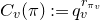
Let
 $C(\pi):=\prod_{v}C_v(\pi)$
be the analytic conductor of
 $\pi,$
where each local conductor
 $C_v(\pi)$
is defined as follows.
-
– For
$v \lt \infty$
, denote by
$r_{\pi_v} \geqslant 0$
the conductor exponent of
$\pi_v$
, which is the unique integer such that
$\pi_v$
has a vector that is
$K_{0,v}^{\circ}[r_{\pi_v}]$
-invariant (see (1.10)) but not
$K_{0,v}^{\circ}[r_{\pi_v} - 1]$
-invariant. Define the local conductor of
$\pi_v$
by
$C_v(\pi) := q_v^{r_{\pi_v}}$
. -
– For
$v\mid\infty,$
the local L-function of
$\pi_v$
is a product of shifted Gamma factors of the shape
$L_v(s,\pi_v)=\Gamma_v(s+\beta_{1,v})\Gamma_v(s+\beta_{2,v}).$
Here,
$\Gamma_v$
is the Gamma function over
$F_v$
, and
$\beta_{1,v}$
and
$\beta_{2,v}$
are complex numbers. Let
\begin{align*} C_v(\pi):=[(1+|\beta_{1,v}|)(1+|\beta_{2,v}|)]^{[F_v:\mathbb{R}]}. \end{align*}




Finally, define
 $C_{{\rm fin}}(\chi) := \prod_{v \lt \infty} C_v(\chi)$
and
 $C_{{\rm fin}}(\pi) := \prod_{v \lt \infty} C_v(\pi)$
as the arithmetic conductors of
 $\chi$
and
 $\pi$
, respectively. Similarly, let
 $C_{\infty}(\chi) := \prod_{v \mid \infty} C_v(\chi)$
and
 $C_{\infty}(\pi) := \prod_{v \mid \infty} C_v(\pi)$
be the Archimedean conductors of
 $\chi$
and
 $\pi$
, respectively.
2.1.2 Types of Archimedean parameters.
Let
 $v \mid \infty$
. For an admissible irreducible representation
 $\Pi_v$
of
 $G(F_v)$
, we denote its associated L-factor by
 \[L_v(s, \Pi_v) = \Gamma_v(s + \gamma_{1,v}) \Gamma_v(s + \gamma_{2,v}). \]
Definition 2.1. Let
 $ 0 \lt \varepsilon_1 \lt 1 $
be a fixed parameter. We say that
 $ \Pi_v $
is of type I relative to
 $\varepsilon_1$
if its parameters
 $\gamma_{1,v}$
and
 $\gamma_{2,v}$
satisfy
 \[\varepsilon_1 |\gamma_{2,v}| \leqslant |\gamma_{1,v}| \leqslant \varepsilon_1^{-1} |\gamma_{2,v}|. \]
Otherwise, we say that
 $ \Pi_v $
is of type II relative to
 $\varepsilon_1$
. Since
 $\varepsilon_1$
is a fixed small number, we will simply say that
 $ \Pi_v $
is of type I or type II, omitting ‘relative to
 $\varepsilon_1$
.’
Let
 $C_v(\pi \otimes \chi)$
be the local conductor defined analogously to
 $C_v(\pi)$
. Let
 $\varepsilon_0\gt0$
be a fixed constant, chosen sufficiently small. Define
 \begin{equation}T_v :=\begin{cases}100 C_v(\pi \otimes \chi)^{\frac{1}{2}} & \text{if } \pi_v \otimes \chi_v \text{ is of type I}, \\\varepsilon_0^{-100}C_v(\pi \otimes \chi) & \text{if } \pi_v \otimes \chi_v \text{ is of type II},\end{cases}\end{equation}
and
 \begin{equation}\iota_v:=\begin{cases}0 & \text{if } \pi_v \otimes \chi_v \text{ is of type I}, \\1/2 & \text{if } \pi_v \otimes \chi_v \text{ is of type II}.\end{cases}\end{equation}
Remark 2.2.
-
(i) The representation
$\pi_v \otimes \chi_v$
is of type I in many favorable situations, such as when
$\pi_v$
is fixed while
$\chi_v$
varies, as in Theorem 1.1, or when
$\pi_v$
varies with a fixed central character while
$\chi_v$
remains constant. -
(ii) If
$\pi_v\otimes\chi_v$
is of type II, then
$C_v(\chi)\leqslant 100\varepsilon_1C_v(\pi).$


2.1.3 Ramification parameters.
For
 $v\in\Sigma_{F,\operatorname{fin}},$
let
 $r_{\chi_v}$
(respectively,
 $r_{\omega_v}$
) be the conductor exponent of
 $\chi_v$
(respectively,
 $\omega_v$
). Let
 $r_{\pi_v}$
be the conductor exponent of
 $\pi_v.$
We set
 \begin{equation}m_v:=\max\{r_{\pi_v},n_v+r_{\omega_v}\}\geqslant n_v:=r_{\chi_v}.\end{equation}
This choice of
 $m_v$
is adopted from [Reference Blomer and HarcosBH14] and offers simplifications in certain local calculations when
 $\omega_v$
is nontrivial.
Define
 $\mathfrak{Q}=\prod_{v\lt\infty}\mathfrak{p}_v^{n_v}$
. For simplicity, we write
 $Q=C_{{\rm fin}}(\chi),$
 $M=C_{{\rm fin}}(\pi),$
and
 $M'=C_{{\rm fin}}(\omega).$
Then
 $M'\mid M.$
2.1.4 Auxiliary finite places.
Let
 $v_0$
and
 $v_1$
be two fixed unramified primes such that
 $q_{v_0}\gt10^{64}$
, and
 $\pi_{v}$
and
 $\chi_{v}$
are unramified at
 $v\in \{v_0,v_1\}$
. Hence,
 $m_{v_0}=n_{v_0}=m_{v_1}=n_{v_1}=0$
.
2.1.5 Hecke operators.
Let
 $\pi=\otimes_{v}\pi_v$
be an automorphic representation of
 $G(\mathbb{A}_F)$
, with central character
 $\omega=\otimes_{v}\omega_v$
. Let
 $\mathfrak{n}$
be an integral ideal in F with primary decomposition
 $\mathfrak{n}=\prod_{v\mid\mathfrak{n}}\mathfrak{p}_v^{l_v}$
. The
 $\mathfrak{p}_v^{l_v}$
th Hecke operator is defined by
 \begin{align*}T_{\mathfrak{p}_v^{l_v}}(\varphi):=q_v^{-{l_v}/{2}}\sum_{\substack{i+j=l_v\\i\geqslant j\geqslant0}}\int_{K_v{\operatorname{diag}}(\varpi_v^{i},\varpi_v^j)K_v}\pi_v(y_v)\varphi\, dy_v,\quad \varphi\in \pi.\end{align*}
Let
 $T_{\mathfrak{n}}(\varphi) := \prod_{v \mid \mathfrak{n}} T_{\mathfrak{p}_v^{l_v}}(\varphi)$
. When
 $\varphi$
is right-invariant under
 $\prod_{v \mid \mathfrak{n}} K_v$
, it becomes an eigenform for the operators
 $T_{\mathfrak{n}}$
and
 $T_{\mathfrak{p}_v^{l_v}}$
for each
 $v \mid \mathfrak{n}$
, with eigenvalues
 $\lambda_{\pi}(\mathfrak{n})$
and
 $\lambda_{\pi}(\mathfrak{p}_v^{l_v})$
, respectively. Moreover, we have
 $\lambda_{\pi}(\mathfrak{n}) = \prod_{v \mid\mathfrak{n}}\lambda_{\pi}(\mathfrak{p}_v^{l_v})$
.
2.1.6 Hecke relations.
Let
 $v\lt\infty$
,
 $l_v\geqslant 0$
and
 $l_v'\geqslant 0$
. We have
 \begin{equation}\overline{\lambda_{\pi}(\mathfrak{p}_v^{l_v})}=\omega_v^{-1}(\varpi_v^{l_v})\cdot \lambda_{\pi}(\mathfrak{p}_v^{l_v}),\end{equation}
and the Hecke relation
 \begin{equation}\lambda_{\pi}(\mathfrak{p}_v^{l_v})\lambda_{\pi}(\mathfrak{p}_v^{l_v'})=\sum_{j=0}^{\min\{l_v,l_v'\}}\omega_v(\varpi_v^{j})\lambda_{\pi}(\mathfrak{p}_v^{l_v+l_v'-2j}).\end{equation}
2.2 Construction of test functions
We shall construct a test function
 $f=\otimes_{v}f_v$
on
 $G(\mathbb{A}_F)$
in the following way.
-
– At Archimedean places
$v\mid\infty$
, we construct
$f_v$
according to the types of
$\pi_{v}\otimes \chi_{v}$
(see § 2.1.2).-
* If
$\pi_v \otimes \chi_v$
is of type I, the function
$f_v$
will be constructed in § 2.2.1 based on Nelson’s work [Reference NelsonNel23] (see §§ 1.5.2 and 14 on p. 80) following the approach in [Reference Nelson and VenkateshNV21, § 1.10] (see also [Reference NelsonNel21, Part 2]). It will sieve out microlocal lifted vectors. -
* If
$\pi_v \otimes \chi_v$
is of type II, the function
$f_v$
will be constructed in § 2.2.2 following the work of Michel and Venkatesh [Reference Michel and VenkateshMV10, § 3.6]. It will sieve out analytic newvectors.
-


Precise constructions will be given in §§ 2.2.1 and 2.2.2.
-
– At the auxiliary fixed finite places
$ v \in \{v_0, v_1\} $
constructed in § 2.1.4, we define
$ f_v $
to simplify the regularized relative trace formula:-
* The local test function
$ f_{v_0} $
defined in § 2.2.3 simplifies the spectral side by annihilating the residues from the continuous spectrum during the regularization. -
* The local test function
$ f_{v_1} $
defined in § 2.2.4 simplifies the geometric side by annihilating certain orbital integrals.
-


Detailed discussions will be provided in §§ 3.4 and 2.4.2.
-
– At ramified finite places, we construct the local test functions via a double average over unipotent translations weighted by characters (see § 2.2.6). This step is essential in handling the level aspect and also simplifies the regularized relative trace formula (see § 2.4.1).
-
– At the remaining places, let
$\mathfrak{n}$
be an integral ideal such that
$\pi_v$
and
$\chi_v$
are unramified for all
$v \mid \mathfrak{n}$
, with
$v_0 \nmid \mathfrak{n}$
and
$v_1 \nmid \mathfrak{n}$
. Define
$f_v$
as follows:-
* For
$v \mid \mathfrak{n}$
, we introduce normalized Hecke operators (following Duke, Friedlander, and Iwaniec [Reference Duke, Friedlander and IwaniecDFI02]) to facilitate further arithmetic amplification. The associated local test functions
$f_v$
, constructed in § 2.2.5, play a crucial role in § 7 to prove Theorem 1.6. -
* For
$v \nmid \mathfrak{n}$
, we take
$f_v$
to be the standard spherical vector.
-


2.2.1 Construction of
${f}_{\infty}$
: the type I case

Let
 $v\mid\infty.$
Suppose that
 $\pi_v\otimes\chi_v$
is of type I. Let
 $T_v=100 C_v(\pi \otimes \chi)^{\frac{1}{2}}$
be the parameter defined by (2.1).
By [Reference NelsonNel23, § 14] and [Reference Nelson and VenkateshNV21, § 2.5], there exists a function
 $\tilde{f}_{v} \in C_c^{\infty}(G(F_v))$
such that
 \begin{equation} \textrm{supp} \tilde{f}_{v} \subseteq \{ g \in G(F_v) : g = I_{n+1} + O(T_v^{-\varepsilon}),\ \operatorname{Ad}^*(g)\tau = \tau + O(T_v^{-\frac{1}{2} + \varepsilon}) \},\end{equation}
where the operator
 $\pi_{v}(\tilde{f}_{v})$
is approximately a rank-one projector with range spanned by a unit vector microlocalized at some chosen element
 $\tau_v$
in the coadjoint orbit of
 $\pi_v \otimes \chi_v$
.
An explicit construction of
 $\tilde{f}_{v}$
can be found in [Reference NelsonNel23, § 14]. Here, we summarize some basic properties of
 $\tilde{f}_{v}$
as follows. For
 $g \in G(F_v)$
, we may write
 \[g = \begin{pmatrix}a & \;\;b \\c & \;\;d\end{pmatrix} \in G(F_v), \quad g^{-1} = \begin{pmatrix}a' &\;\; b' \\c' &\;\; d'\end{pmatrix} \in G(F_v). \]
Define
 \[d_{v}(g) :=\begin{cases}\min\big\{ 1, |d^{-1}b|_v + |d^{-1}c|_v + |d'^{-1}b'|_v + |d'^{-1}c'|_v \big\} & \text{if $dd' \neq 0,$} \\1 & \text{if $dd' = 0$}.\end{cases} \]
As a consequence of [Reference NelsonNel21, (14.13)] and [Reference NelsonNel23, Theorem 15.1], along with the support constraint (2.6), we obtain
 \begin{equation}|\tilde{f}_v(g)| \ll T_v^{1+\varepsilon} \cdot\mathbf{1}_{|\operatorname{Ad}^*(g)\tau - \tau| \ll T_v^{-1/2+\varepsilon}} \cdot \mathbf{1}_{|g - I_2| \ll T_v^{-\varepsilon}} \cdot \min\bigg\{\! 1, \frac{T_v^{-\frac{1}{2}+\varepsilon}}{d_v(g)} \bigg\}.\end{equation}
We thus define the local test function
 $f_v$
by
 \begin{equation}f_{v}(g) := (f_{v}^{\dagger} * (f_{v}^{\dagger})^*)(g),\end{equation}
where
 $v \mid \infty$
,
 $g \in G(F_v)$
, and
 \begin{equation}f_{v}^{\dagger}(g) := \chi_v(\det g) \int_{F_v^{\times}} \tilde{f}_{v}(zg)\omega_{v}(z) \, d^{\times}z.\end{equation}
Remark 2.3. We do not recall the precise construction of
 $\tilde{f}_{v}$
from [Reference NelsonNel23, 14]; instead, we will only use its relevant properties, with appropriate references to the source.
2.2.2 Construction of
${f}_{\infty}$
: the type II case

Let
 $v\mid\infty$
. Suppose that
 $\pi_v\otimes\chi_v$
is of type II. Let
 $T_v=\varepsilon_0^{-100} C_v(\pi \otimes \chi)$
be the parameter defined by (2.1).
Let
 $ h_{v}^{\varepsilon_0} = (h_{1,v}, h_{2,v}, h_{3,v}) \in C_c^{\infty}(F_v^{\times} \times F_v \times F_v) $
be a triple of nonnegative Schwartz functions with compact support, satisfying the following conditions:
-
–
$ \int_{F_v^{\times}} h_{1,v}(a) \, d^{\times}a = 1 $
,
$ h_{1,v}(a) = 0 $
unless
$ |a - 1|_v \leqslant \varepsilon_0 $
, and
\[h_{1,v}^{(j)}(a) \ll \varepsilon_0^{-j-1} \quad \text{for all } a \in F_v^{\times} \text{ and } 0 \leqslant j \leqslant 2; \]
-
–
$ |\int_{F_v} h_{2,v}(b) \psi_v(b)\, db| = 1 $
, and
$ h_{2,v}(b) = 0 $
unless
$ |b_v|_v \leqslant 10^{-3} $
; and -
–
$ \int_{F_v} h_{3,v}(c) \,dc = 1 $
, and
$ h_{3,v}(c) = 0 $
unless
$ |c|_v \leqslant \varepsilon_0 $
.


Let
 $h_{2,v}'$
be the derivative of
 $h_{2,v}$
. Define
 \begin{equation}\tilde{f}_v(g,h_v^{\varepsilon_0}):=T_v\chi_v(\det g)h_{1,v}(z)h_{1,v}(a)h_{2,v}'(b)h_{3,v}(T_v^{1+\varepsilon}c)\end{equation}
if
 $g=z\big(\!\begin{smallmatrix}a&\;\; b\\& 1\end{smallmatrix}\!\big)\big(\!\begin{smallmatrix}1& \\c &\;\; 1\end{smallmatrix}\!\big)\in G(F_v)$
, and set
 $\tilde{f}_v(g,h_v^{\varepsilon_0})\equiv 0$
otherwise. Define
 \begin{equation}f_{v}^{\dagger}(g):=\chi_v(\det g)T_v^{-\frac{1}{4}}\int_{F_v^{\times}}\tilde{f}_v(zg,h_{v}^{\varepsilon_0})\omega_{v}(z) \, d^{\times}z.\end{equation}
By the Bruhat decomposition, the set
 \begin{align*}\bigg\{g=z\begin{pmatrix}a& \;\;b\\& 1\end{pmatrix}\begin{pmatrix}1& \\c &\;\; 1\end{pmatrix}\in G(F_v):\ a, z\in F_v^{\times},\ b, c\in F_v\!\bigg\}\end{align*}
is open in
 $G(F_v)$
. Consequently, for sufficiently small
 $\varepsilon_0$
, the function
 $f_{v}^{\dagger}(g)$
is smooth and supported in a small neighborhood of the identity matrix
 $I_2$
.
The local test function is then defined by
 \begin{equation}f_v(g)=(f_{v}^{\dagger}*(f_{v}^{\dagger})^*)(g),\quad g\in G(F_v).\end{equation}
2.2.3 Non-Archimedean test function
$f_{v_0}$

Let
 $v_0$
be the fixed unramified place as in § 2.1.4. For
 $v=v_0$
, we define
 \begin{equation}\tilde{h}_v:=\sum_{\beta\in \mathcal{O}_v^{\times}/(1+\mathfrak{p}_v)}\psi_v(\beta\varpi_v^{-1})\mathbf{1}_{u_{\beta}K_v}+\mathbf{1}_{\mathbf{d}K_v},\end{equation}
where
 $u_{\beta}=\big(\!\begin{smallmatrix}1&\;\; \beta\varpi_v^{-1}\\&1\end{smallmatrix}\!\big)$
, and
 $\mathbf{d}:=\operatorname{diag}(\varpi_v^{-1},\varpi_v).$
We define the local test function by
 \begin{equation}f_v(g):=(f_{v}^{\dagger}*(f_{v}^{\dagger})^*)(g),\quad g\in G(F_v),\end{equation}
where
 \begin{equation}f_{v}^{\dagger}(g):=\int_{F_v^{\times}}\tilde{h}_v(gz)\omega_v(z) \, d^{\times}z.\end{equation}
The test function
 $f_v(g_v)$
is introduced to eliminate contributions from the residues of period integrals on the spectral side when shifting contours during the regularization of the relative trace formula (see Proposition 3.1).
2.2.4 Non-Archimedean test function
$f_{v_1}$

Let
 $v=v_1$
be the fixed unramified place as in § 2.1.4. We define the test function by
 \begin{equation}f_v(g_v)=f_{v}^{\dagger}(g):=\begin{cases}\displaystyle\frac{\omega_v(z_v)^{-1}\omega_v(E_{2,2}(k_v))^{-1}}{\operatorname{Vol}(\overline{K_{v}[1]})}&\ \text{if $g_v=z_vk_v\in Z(F_v)K_{v}[1]$,}\\0 &\ \text{otherwise,}\end{cases}\end{equation}
where
 $\overline{K_{0,v}[1]}$
is the image of
 $K_{0,v}[1]$
in
 $\overline{G}(F_v),$
and
 $E_{2,2}(k_v)$
is the (2,2)th entry of
 $k_v\in K_{0,v}[1]$
. We have
 $f_{v}(g)=(f_{v}^{\dagger}*(f_{v}^{\dagger})^*)(g)$
.
2.2.5 Non-Archimedean test function
$f_v$
at
$v\mid\mathfrak{n}$


Let
 $\mathfrak{n}$
be an integral ideal such that
 $\pi_v$
and
 $\chi_v$
are unramified for all
 $v \mid \mathfrak{n}$
, and
 $v_0 \nmid \mathfrak{n}$
and
 $v_1 \nmid \mathfrak{n}$
. For
 $v\mid\mathfrak{n}$
, we define
 \begin{equation}f_v(g):=q_v^{-({e_v(\mathfrak{n})})/{2}}\sum_{\substack{i+j=e_v(\mathfrak{n})\\i\geqslant j\geqslant0}}\int_{F_v^{\times}}\mathbf{1}_{K_v{\operatorname{diag}}(\varpi_v^i,\varpi_v^j)K_v}(zg)\omega_v(z) \, d^{\times}z,\quad g\in G(F_v).\end{equation}
2.2.6 Non-Archimedean test function
$f_v$
: the remaining places

For
 $v\in\Sigma_{F,\operatorname{fin}}-\{v_0,v_1\}$
such that
 $v\nmid\mathfrak{n}$
, we define
 \begin{equation}f_{v}^{\dagger}(g):=\frac{1}{\operatorname{Vol}(\overline{K_{0,v}[m_v]})}\int_{F_v^{\times}}\mathbf{1}_{K_{0,v}[m_v]}(zg)\omega_v(z) \, d^{\times}z,\end{equation}
where
 $\overline{K_{0,v}[m_v]}$
is the image of
 $K_{0,v}[m_v]$
in
 $\overline{G}(F_v)$
. For
 $g\in G(F_v),$
define by
 \begin{equation}f_v(g)=\frac{1}{|\tau(\chi_v)|^{2}}\sum_{\substack{\alpha\in \mathcal{O}_v^{\times}/(1+\varpi_v^{n_v}\mathcal{O}_v^{\times})\\\beta\in \mathcal{O}_v^{\times}/(1+\varpi_v^{n_v}\mathcal{O}_v^{\times})}}\chi_v(\alpha)\overline{\chi}_v(\beta)f_{v}^{\dagger}(g_{\alpha,\beta}),\end{equation}
where
 $$\tau(\chi_v)=\sum_{\alpha\in \mathcal{O}_v^{\times}/(1+\varpi_v^{n_v}\mathcal{O}_v^{\times})}\psi_v(\alpha\varpi_v^{-n_v})\chi_v(\alpha)$$
is the Gauss sum relative to the additive character
 $\psi_v$
, and
 \begin{align*} g_{\alpha,\beta}:=\begin{pmatrix} 1&\;\;\alpha \varpi_v^{-n_v}\\ &1 \end{pmatrix}g\begin{pmatrix} 1&\;\;\beta \varpi_v^{-n_v}\\ &1 \end{pmatrix}\!.\end{align*}
Here, we identify
 $\alpha, \beta \in \mathcal{O}_v^{\times}/(1 + \varpi_v^{n_v} \mathcal{O}_v^{\times})$
with their representatives in
 $\mathcal{O}_v^{\times}$
to ensure that
 $g_{\alpha, \beta} \in G(F_v)$
.
Note that
 $n_v = 0$
for almost all
 $v \in \Sigma_{F, \mathrm{fin}}$
. Consequently, for all but finitely many
 $v \in \Sigma_{F, \mathrm{fin}}$
, we have
 $f_v=f_{v}^{\dagger}=f_{v}^{\dagger}*(f_{v}^{\dagger})^*$
, supported on
 $Z(F_v) K_{0,v}[m_v]$
.
By definition (2.3), we have
 $ m_v = 0 $
for
 $ v \in \{v_0, v_1\} $
and
 $v\mid\mathfrak{n}$
.


2.3 Decomposition of the kernel function
Let f be the test function defined in § 2.2.7. Then f defines an integral operator
 \begin{equation} R(f)\phi(g) = \int_{\overline{G}(\mathbb{A}_F)} f(g')\phi(gg') \, dg'\end{equation}
on the space
 $L^2([G], \omega )$
of functions on [G] that transform under
 $Z(\mathbb{A}_F)$
by
 $\omega$
and are square-integrable on
 $[\overline{G}]$
.
By making the change of variable
 $g' \mapsto g^{-1}g'$
in (2.20), and using the fact that
 $\phi$
is left-G(F)-invariant, we obtain
 \[R(f)\phi(g) = \int_{[\overline{G}]} \operatorname{K}(g, g')\phi(g') \, dg', \]
where for
 $g_1, g_2 \in G(\mathbb{A}_F)$
,
 \begin{equation}\operatorname{K}(g_1, g_2) := \sum_{\gamma \in \overline{G}(F)} f(g_1^{-1} \gamma g_2)\end{equation}
is the kernel function of R(f). Since f has compact support modulo the center, the sum in (2.21) converges absolutely.
It is well-known that
 $L^2([G],\omega)$
decomposes into the direct sum of the space
 $L_0^2([G],\omega)$
of cusp forms and spaces
 $L_{{\rm Eis}}^2([G],\omega)$
and
 $L_{{\rm Res}}^2([G],\omega)$
defined in terms of Eisenstein series and residues of Eisenstein series, respectively.
Let R be the right regular representation of
 $G(\mathbb{A}_F)$
on
 $L^2([G],\omega)$
. The spectral decomposition of the
 $L^2([G],\omega)$
(see [Reference Gelbart and JacquetGJ79]) gives that
 \begin{equation}R=\bigoplus_{\text{$\sigma$ cuspidal}}\sigma \oplus \int_{i\mathbb{R}}\bigoplus_{\eta\in\widehat{F^{\times}\backslash \mathbb{A}_F^{(1)}}}\sigma_{\lambda,\eta}\frac{d\lambda}{4\pi i} \oplus \bigoplus_{\substack{\eta\in \widehat{F^{\times}\backslash\mathbb{A}_F^{(1)}}\\ \eta^2=\omega}}\eta\circ \det,\end{equation}
where
 $\sigma_{\lambda,\eta}=\operatorname{Ind}(\eta|\cdot|^{\lambda},\eta^{-1}\omega|\cdot|^{-\lambda})$
denotes the normalized parabolic induction of the characters
 $\eta|\cdot|^{\lambda}$
and
 $\eta^{-1}\omega|\cdot|^{-\lambda}$
.
Then the kernel function
 $\operatorname{K}(g_1,g_2)$
decomposes as the pre-trace formula:
 \begin{equation} \operatorname{K}_0(g_1,g_2)+\operatorname{K}_{{\rm ER}}(g_1,g_2)=\operatorname{K}(g_1,g_2)=\sum_{\gamma\in \overline{G}(F)}f(g_1^{-1}\gamma g_2),\end{equation}
where
 $\operatorname{K}_0$
is the contribution from the cuspidal spectrum, and
 $\operatorname{K}_{{\rm ER}}(g_1,g_2)$
is the contribution from the noncuspidal spectrum. The subscript ‘
 $\operatorname{ER}$
’ refers to Eisenstein series and their residues. Explicit expansions of
 $\operatorname{K}_0(g_1,g_2)$
and
 $\operatorname{K}_{{\rm ER}}(g_1,g_2)$
will be given in § 3.2.
Substituting the Bruhat decomposition
 \begin{align*}\overline{G}(F)=B_0(F)\bigsqcup B_0(F)wN(F),\quad w=\begin{pmatrix}&\;\; 1\\1\end{pmatrix}\end{align*}
into (2.21), we obtain
 $\operatorname{K}(g_1,g_2)=\operatorname{K}_{{\rm Small}}(g_1,g_2)+\operatorname{K}_{{\rm Big}}(g_1, g_2),$
where
 \begin{align*} \operatorname{K}_{{\rm Small}}(g_1,g_2)=\sum_{\gamma\in B_0(F)}f(g_1^{-1}\gamma g_2),\quad \operatorname{K}_{{\rm Big}}(g_1,g_2)=\sum_{\gamma\in B_0(F)wN(F)}f(g_1^{-1}\gamma g_2). \end{align*}
Let
 $\mathcal{K}(\cdot,\cdot)\in \{\operatorname{K}(\cdot,\cdot), \operatorname{K}_0(\cdot,\cdot), \operatorname{K}_{{\rm ER}}(\cdot,\cdot), \operatorname{K}_{{\rm Small}}(\cdot,\cdot),\operatorname{K}_{{\rm Big}}(\cdot,\cdot)\}.$
Define
 \begin{align*}\mathcal{F}_0\mathcal{F}_1\mathcal{K}(g_1,g_2)&:=\int_{[N]}\mathcal{K}(g_1,u_2g_2) \, du_2,\quad \mathcal{F}_1\mathcal{F}_0\mathcal{K}(g_1,g_2):=\int_{[N]}\mathcal{K}(u_1g_1,g_2) \, du_1,\\\mathcal{F}_1\mathcal{F}_1\mathcal{K}(g_1,g_2)&:=\int_{[N]}\int_{[N]}\mathcal{K}(u_1g_1,u_2g_2) \, du_2 \, du_1,\\\mathcal{F}_2\mathcal{F}_2\mathcal{K}(g_1,g_2)&:=\sum_{\alpha\in A(F)}\sum_{\beta\in A(F)}\int_{[N]}\int_{[N]}\mathcal{K}(u_1\alpha g_1,u_2\beta g_2)\theta(u_1)\overline{\theta}(u_2) \, du_2 \, du_1.\end{align*}
Using the Poisson summation twice yields
 \begin{align}\mathcal{F}_2\mathcal{F}_2\mathcal{K}(g_1,g_2)=\mathcal{K}(g_1,g_2)-\mathcal{F}_0\mathcal{F}_1\mathcal{K}(g_1,g_2)-\mathcal{F}_1\mathcal{F}_0\mathcal{K}(g_1,g_2)+\mathcal{F}_1\mathcal{F}_1\mathcal{K}(g_1,g_2).\end{align}
Since f has compact support modulo the center, (2.24) converges absolutely.
Lemma 2.4.
For
 $x, y\in A(\mathbb{A}_F)$
, we have
 \begin{align*}\mathcal{F}_0\mathcal{F}_1\operatorname{K}_{{\rm Big}}(x,y)=\mathcal{F}_1\mathcal{F}_0\operatorname{K}_{{\rm Big}}(x,y)=\mathcal{F}_1\mathcal{F}_1\operatorname{K}_{{\rm Big}}(x,y)\equiv 0.\end{align*}
Proof. By the definition of
 $\operatorname{K}_{{\rm Big}}(\cdot,\cdot)$
,
 \begin{align*}\mathcal{F}_0\mathcal{F}_1\operatorname{K}_{{\rm Big}}(x,y)=\sum_{b\in B_0(F)}\int_{N(\mathbb{A})}f(x^{-1}bwu_2y) \, du_2.\end{align*}
Now let
 $v\mid\mathfrak{Q}$
, so that
 $n_v\geqslant 1.$
By the definition of
 $f_v$
, we have
 \begin{align}&|\tau(\chi_v)|^2 \int_{N(F_v)} f_v(x_{v}^{-1} b w u_{v} y_{v}) \,du_{v}\nonumber\\&\quad = \sum_{\alpha, \beta \in \mathcal{O}_v^{\times} / (1 + \varpi_v^{n_v} \mathcal{O}_v^{\times})}\chi_v(\alpha) \overline{\chi}_v(\beta)\int_{N(F_v)}f_v^{\dagger} \bigg(\!\!\begin{pmatrix} 1 &\;\; \alpha \varpi_v^{n_v} \\ & 1\end{pmatrix}x_{v}^{-1} b w u_{v} y_{v}\begin{pmatrix} 1 & \;\;\beta \varpi_v^{n_v} \\ & 1\end{pmatrix}\!\!\bigg) \, du_{v},\end{align}
where the local test function
 $f_{v}^{\dagger}(\cdot)$
is defined by (2.18).
Since
 $y_{v} \in A(F_v)$
, after the change of variables
 \[u_{v} \mapsto u_{v} y_{v}\begin{pmatrix} 1 &\;\; -\beta q_v^{n_v} \\ & 1\end{pmatrix}y_{v}^{-1}, \]
the right-hand side of (2.25) becomes
 \begin{align*}\sum_{\beta \in \mathcal{O}_v^{\times} / (1 + \varpi_v^{n_v} \mathcal{O}_v^{\times})}\overline{\chi}_v(\beta)\sum_{\alpha \in \mathcal{O}_v^{\times} / (1 + \varpi_v^{n_v} \mathcal{O}_v^{\times})}\chi_v(\alpha)\int f_v^{\dagger} \bigg(\!\!\begin{pmatrix} 1 &\;\; \alpha q_v^{n_v} \\ & 1\end{pmatrix}x_{v}^{-1} b w u_{v} y_{v}\!\bigg) \, du_{v},\end{align*}
which vanishes as a consequence of the character orthogonality
 \[\sum_{\beta \in \mathcal{O}_v^{\times} / (1 + \varpi_v^{n_v} \mathcal{O}_v^{\times})}\overline{\chi}_v(\beta) = 0. \]
Hence (2.25) vanishes, which implies that
 $\mathcal{F}_0\mathcal{F}_1\operatorname{K}_{{\rm Big}}(x,y)=0.$
Likewise, we have
 $\mathcal{F}_1\mathcal{F}_0\operatorname{K}_{{\rm Big}}(x,y)=\mathcal{F}_1\mathcal{F}_1\operatorname{K}_{{\rm Big}}(x,y)=0.$
2.4 The regularized relative trace formula
Let
 $\textbf{s}=(s_1, s_2)\in\mathbb{C}^2,$
with
 ${\rm Re}(s_1)\ggg 1$
and
 ${\rm Re}(s_2)\ggg 1.$
Consider the integral
 \begin{equation}\int_{[A]}\int_{[A]}\mathcal{F}_2\mathcal{F}_2\operatorname{K}(x,y)|\det x|^{s_1}|\det y|^{s_2}\chi(x)\overline{\chi}(y) \, d^{\times}x \, d^{\times}y.\end{equation}
It follows from [Reference YangYan23, § 6.2] that the above integral converges absolutely when
 ${\rm Re}(s_1)$
and
 ${\rm Re}(s_2)$
are sufficiently large.
We denote by
 $J_{\textrm{Spec}}^{{\rm Reg}}(f,\mathbf{s},\chi)$
the integral (2.26) obtained by substituting the spectral expansion
 $\operatorname{K}(g_1,g_2)= \operatorname{K}_0(g_1,g_2)+\operatorname{K}_{{\rm ER}}(g_1,g_2)$
into it. Likewise, we denote by
 $J_{{\rm Geo}}^{{\rm Reg}}(f,\mathbf{s},\chi)$
the integral obtained by substituting the geometric expansion (2.21) into (2.26). As a consequence, we have the coarse relative trace formula
 \begin{equation}J_{\textrm{Spec}}^{{\rm Reg}}(f,\mathbf{s},\chi)=J_{{\rm Geo}}^{{\rm Reg}}(f,\mathbf{s},\chi),\end{equation}
where
 ${\rm Re}(s_1)$
and
 ${\rm Re}(s_2)$
are sufficiently large.
For convenience, we refer to
 $J_{\textrm{Spec}}^{{\rm Reg}}(f,\mathbf{s},\chi)$
as the spectral side of the relative trace formula and
 $J_{{\rm Geo}}^{{\rm Reg}}(f,\mathbf{s},\chi)$
as the geometric side of the relative trace formula.
2.4.1 The spectral side.
Let
 $\textbf{s}=(s_1, s_2)\in\mathbb{C}^2,$
with
 ${\rm Re}(s_1)\ggg 1$
and
 ${\rm Re}(s_2)\ggg 1.$
Note that
 $\operatorname{K}_0(x,y)=\mathcal{F}_2\mathcal{F}_2\operatorname{K}_0(x,y).$
By the definition (2.26), we have
 \begin{equation}J_{\textrm{Spec}}^{{\rm Reg}}(f,\textbf{s},\chi)=J_{0}^{{\rm Reg}}(f,\textbf{s},\chi)+J_{{\rm Eis}}^{{\rm Reg}}(f,\textbf{s},\chi),\end{equation}
where
 \begin{align*}J_{0}^{{\rm Reg}}(f,\textbf{s},\chi)&:=\int_{[A]}\int_{[A]}\operatorname{K}_0(x,y)|\det x|^{s_1}|\det y|^{s_2}\chi(x)\overline{\chi}(y) \, d^{\times}x \, d^{\times}y,\\J_{{\rm Eis}}^{{\rm Reg}}(f,\textbf{s},\chi)&:=\int_{[A]}\int_{[A]}\mathcal{F}_2\mathcal{F}_2\operatorname{K}_{{\rm ER}}(x,y)|\det x|^{s_1}|\det y|^{s_2}\chi(x)\overline{\chi}(y) \, d^{\times}x \, d^{\times}y.\end{align*}
In § 3 we will show that the spectral side
 $J_{\textrm{Spec}}^{{\rm Reg}}(f,\textbf{s},\chi)$
admits a holomorphic continuation
 $J_{\textrm{Spec}}^{{\rm Reg},\heartsuit}(f,\textbf{s},\chi)$
to the region
 $-1/4\lt{\rm Re}(s_1),\ {\rm Re}(s_2)\lt1/4$
.
2.4.2 The geometric side.
Let
 ${\rm Re}(s_1)\ggg 1$
and
 ${\rm Re}(s_2)\ggg 1$
. By (2.24), Lemma 2.4, and the Bruhat decomposition
 $\operatorname{K}(x,y)=\operatorname{K}_{{\rm Small}}(x,y)+\operatorname{K}_{{\rm Big}}(x,y),$
we have
 \begin{equation}J_{{\rm Geo}}^{{\rm Reg}}(f,\textbf{s},\chi)=J^{{\rm Reg}}_{{\rm Geo},{\rm Small}}(f,\textbf{s},\chi)+J^{{\rm Reg}}_{{\rm Geo},{\rm Big}}(f,\textbf{s},\chi),\end{equation}
where
 \begin{align*}J^{{\rm Reg}}_{{\rm Geo},{\rm Small}}(f,\textbf{s},\chi)&:=\int_{[A]}\int_{[A]}\mathcal{F}_2\mathcal{F}_2\operatorname{K}_{{\rm Small}}(x,y)|\det x|^{s_1}|\det y|^{s_2}\chi(x)\overline{\chi}(y) \, d^{\times}x \, d^{\times}y,\\J^{{\rm Reg}}_{{\rm Geo},{\rm Big}}(f,\textbf{s},\chi)&:=\int_{[A]}\int_{[A]}\operatorname{K}_{{\rm Big}}(x,y)|\det x|^{s_1}|\det y|^{s_2}\chi(x)\overline{\chi}(y) \, d^{\times}x \, d^{\times}y.\end{align*}
In view of the construction of
 $f_{v_1}$
in (2.16), we deduce from [Reference YangYan23, § 5] (or from the proof in [Reference Ramakrishnan and RogawskiRR05]) that
 \begin{equation}J^{{\rm Reg}}_{{\rm Geo},{\rm Big}}(f,\textbf{s},\chi)=J^{{\rm Reg}}_{{\rm Geo},{\rm Dual}}(f,\textbf{s},\chi)+J^{{\rm Reg},II}_{{\rm Geo},{\rm Big}}(f,\textbf{s},\chi),\end{equation}
where
 $J_{{\rm Geo},{\rm Dual}}^{{\rm Big}}(f,\textbf{s},\chi)$
is defined by
 \begin{equation}\int_{\mathbb{A}_F^{\times}}\int_{\mathbb{A}_F^{\times}}f\bigg(\!\!\begin{pmatrix} 1\\ x&\;\;1\end{pmatrix}\begin{pmatrix} y\\ &\;\;1\end{pmatrix}\!\!\bigg)|x|^{s_1+s_2}|y|^{s_2}\overline{\chi}(y) \, d^{\times}y \, d^{\times}x,\end{equation}
and the regular orbital
 $J^{{\rm Reg},II}_{{\rm Geo},{\rm Big}}(f,\textbf{s},\chi)$
is defined by
 \begin{equation}\sum_{t\in F-\{0,1\}}\int_{\mathbb{A}_F^{\times}}\int_{\mathbb{A}_F^{\times}}f\bigg(\!\!\begin{pmatrix} y&\;\;x^{-1}t\\ xy&1\end{pmatrix}\!\!\bigg)|x|^{s_1+s_2}|y|^{s_2}\overline{\chi}(y) \, d^{\times}y \, d^{\times}x.\end{equation}
Remark 2.5. Without the component
 $f_{v_1}$
, the decomposition (2.29) may include additional terms. For instance, if
 $\pi$
and
 $\chi$
are both unramified at all finite places (i.e.,
 $m_v = 0$
for all
 $v \lt \infty$
, e.g.,
 $\chi=|\cdot|^{it}$
), then there are two extra terms in (2.30) (see [Reference Wei, Yang and ZhaoWYZ24, § 2.2.3]).
Since f is a Schwartz–Bruhat function, Tate’s thesis implies that
 $J_{{\rm Geo},{\rm Dual}}^{{\rm Big}}(f,\mathbf{s},\chi)$
converges absolutely for
 ${\rm Re}(s_1 + s_2) \gt 1$
, and it represents the complete Dedekind
 $\zeta$
-function
 $\Lambda(s_1 + s_2)$
. Likewise,
 $J^{{\rm Reg}}_{{\rm Geo},{\rm Small}}(f,\textbf{s},\chi)$
is a Tate integral representing
 $\Lambda(1+s_1 + s_2)$
. Moreover, by Theorem 5.6 in [Reference YangYan23, § 5.4], the integral
 $J^{{\rm Reg},II}_{{\rm Geo},{\rm Big}}(f,\mathbf{s},\chi)$
converges absolutely for all
 $\mathbf{s}\in\mathbb{C}^2$
. In particular, the sum over
 $t \in F \setminus \{0,1\}$
is finite, a property referred to as stability of the regular orbital integrals (see [Reference Feigon and WhitehouseFW09, Reference Michel and RamakrishnanMR12]).
Throughout §§ 4–6, we give detailed quantitative descriptions of the functions
 $J^{{\rm Reg}}_{{\rm Geo},{\rm Small}}(f,\mathbf{s},\chi)$
,
 $J^{{\rm Reg}}_{{\rm Geo},{\rm Dual}}(f,\mathbf{s},\chi)$
, and
 $J^{{\rm Reg},II}_{{\rm Geo},{\rm Big}}(f,\mathbf{s},\chi)$
. As a result, we obtain a holomorphic continuation
 $J_{{\rm Geo}}^{{\rm Reg},\heartsuit}(f,\mathbf{s},\chi)$
of
 $J_{{\rm Geo}}^{{\rm Reg}}(f,\mathbf{s},\chi)$
to
 $\mathbf{s}\in\mathbb{C}^2.$
2.4.3 The relative trace formula.
Let
 $J_{\textrm{Spec}}^{{\rm Reg},\heartsuit}(f,\mathbf{s},\chi)$
and
 $J_{{\rm Geo}}^{{\rm Reg},\heartsuit}(f,\mathbf{s},\chi)$
be the holomorphic continuations of
 $J_{\textrm{Spec}}^{{\rm Reg}}(f,\mathbf{s},\chi)$
and
 $J_{{\rm Geo}}^{{\rm Reg}}(f,\mathbf{s},\chi)$
, respectively. As a consequence of (2.27), we obtain the following.
Theorem 2.6.
Let
 $\varepsilon\gt0$
be a small constant. Let
 $\mathcal{C}:=\{s\in\mathbb{C}:\ |s|=\varepsilon\}$
be the circle of radius
 $\varepsilon$
. Let
 $\mathbf{s}=(s,0)$
. Then
 \begin{align}J_{\textrm{Spec}}^{{\rm Reg},\heartsuit}(f,\mathbf{0},\chi)&=\frac{1}{2\pi i}\int_{\mathcal{C}}\frac{J^{{\rm Reg}}_{{\rm Geo},{\rm Small}}(f,\mathbf{s},\chi)}{s} \, ds\nonumber\\&\quad +\frac{1}{2\pi i}\int_{\mathcal{C}}\frac{J^{{\rm Reg}}_{{\rm Geo},{\rm Dual}}(f,\mathbf{s},\chi)}{s} \, ds+J^{{\rm Reg},II}_{{\rm Geo},{\rm Big}}(f,\textbf{0},\chi).\end{align}
Here,
 $J^{{\rm Reg}}_{{\rm Geo},{\rm Small}}(f,\mathbf{s},\chi)$
and
 $J^{{\rm Reg}}_{{\rm Geo},{\rm Dual}}(f,\mathbf{s},\chi)$
are understood via their meromorphic continuation, as established by Tate’s thesis.
A more precise form of the formula (2.33) will be developed in §§ 3–6.
3. The spectral side: meromorphic continuation and bounds
Let
 $\mathbf{s}=(s_1,s_2)$
. In this section, we shall show that
 $J_{\textrm{Spec}}^{{\rm Reg}}(f,\textbf{s},\chi)$
admits a meromorphic continuation
 $J_{\textrm{Spec}}^{{\rm Reg},\heartsuit}(f,\textbf{s},\chi)$
to the region
 $-1/4\lt{\rm Re}(s_1),\ {\rm Re}(s_2)\lt1/4$
.
3.1 Eisenstein series
Define
 $H_T: T(\mathbb{A}_F)\rightarrow\mathbb{R}$
by setting
 $H\big(\!\big(\begin{smallmatrix} a\\ &\;\;d\end{smallmatrix}\big)\!\big)=\log |ad^{-1}|_{\mathbb{A}_F}.$
Extend
 $H_T$
to a map
 $H: G(\mathbb{A}_F)\rightarrow\mathbb{R}$
by using the Iwasawa decomposition
 $G(\mathbb{A}_F)=N(\mathbb{A}_F)T(\mathbb{A}_F)K,$
and defining
 $H(utk)=H_T(t),$
 $u\in N(\mathbb{A}_F),$
 $t\in T(\mathbb{A}_F),$
and
 $k\in K.$
For
 $\eta\in \widehat{F^{\times}\backslash\mathbb{A}_F^{(1)}}$
and
 $\lambda\in \mathbb{C}$
, let
 $\sigma_{\lambda,\eta}=\operatorname{Ind}(\eta|\cdot|^{\lambda},\eta^{-1}\omega|\cdot|^{-\lambda})$
be the parabolic induction. Let
 $\phi\in\sigma_{0,\eta}$
be a section. Define the Eisenstein series
 \begin{align*}E(g,\phi,\lambda)=\sum_{\delta\in B(F)\backslash G(F)}\phi(\delta g)e^{(\frac{1}{2}+\lambda)H(\delta g)},\quad {\rm Re}(\lambda)\gt1.\end{align*}
Then
 $E(g,\phi,\lambda)$
converges absolutely and admits a meromorphic continuation to
 $\lambda\in\mathbb{C}$
with possible simple poles at
 $\lambda\in \{0,1\}$
, as well as a functional equation.
Let f be constructed in § 2.2. For
 $g\in G(\mathbb{A}_F),$
define
 \begin{align*}E(g,\mathcal{I}(\lambda, f)\phi,\lambda)=\sigma_{0,\eta}(f)E(g,\phi,\lambda):=\int_{\overline{G}(\mathbb{A}_F)}f(y)E(gy,\phi,\lambda) \, dy,\quad {\rm Re}(\lambda)\gt1.\end{align*}
To simplify the notation, we also use
 $E(g,\phi,\lambda)$
and
 $E(g,\mathcal{I}(\lambda, f)\phi,\lambda)$
to denote their meromorphic continuations.
3.2 Spectral expansion of the kernel functions
Let the notation be as in § 2.2. Define
 $\operatorname{K}_0(x, y)$
and
 $\operatorname{K}_{{\rm ER}}(x, y)$
by (2.23). Then, by the decomposition (2.22),
 \begin{align*}\operatorname{K}_0(x, y) &= \sum_{\sigma \in \mathcal{A}_0([G], \omega)} \sum_{\phi \in \mathfrak{B}_{\sigma}} \sigma(f) \phi(x) \overline{\phi(y)},\\\operatorname{K}_{{\rm ER}}(x, y) &= \frac{1}{4\pi} \sum_{\eta \in \widehat{F^{\times} \backslash \mathbb{A}_F^{(1)}}} \int_{i\mathbb{R}}\sum_{\phi \in \mathfrak{B}_{\sigma_{0,\eta}}}E(x, \mathcal{I}(\lambda, f)\phi, \lambda)\overline{E(y, \phi, \lambda)} \, d\lambda,\end{align*}
where
 $\mathfrak{B}_{\sigma}$
and
 $\mathfrak{B}_{\sigma_{0,\eta}}$
are orthonormal bases of
 $\sigma$
and
 $\sigma_{0,\eta} = \operatorname{Ind}(\eta, \eta^{-1} \omega)$
with respect to their associated inner products, respectively.
According to the construction in § 2.2, the test function f is right invariant under
 \begin{equation}K[\ast]:=K_{v_1}[1]\bigotimes \prod_{v\lt\infty,\ v\neq v_1}K_{0,v}[m_v].\end{equation}
Hence, we may take
 $\phi\in\mathfrak{B}_{\sigma}^{K[\ast]}$
and
 $\phi\in \mathfrak{B}_{\sigma_{0,\eta}}^{K[\ast]}$
in the above definitions of
 $\operatorname{K}_0(x,y)$
and
 $\operatorname{K}_{{\rm ER}}(x,y)$
, respectively. Here,
 $\mathfrak{B}_{\sigma}^{K[\ast]}$
(respectively,
 $\mathfrak{B}_{\sigma_{0,\eta}}^{K[\ast]}$
) consists of vectors in
 $\mathfrak{B}_{\sigma}$
that are right-
 $K[\ast]$
-invariant modulo the center.
3.3 Rankin–Selberg periods
Let
 $\varphi$
be a generic automorphic form on
 $G(\mathbb{A}_F).$
Define the associated Whittaker function by
 \begin{equation}W_{\varphi}(g):=\int_{[N]}\varphi(ug)\overline{\theta(u)} \, du,\quad g\in G(\mathbb{A}_F),\end{equation}
where
 $\theta=\otimes_v\theta_v$
is the generic additive character of
 $N(\mathbb{A}_F)$
.
By multiplicity one,
 $W_{\varphi}$
factors into local integrals, i.e.,
 $W_{\varphi}(g)=\prod_{v}W_{\varphi,v}(g_v),$
where
 $g=\otimes_{v}g_v\in G(\mathbb{A}_F)$
and
 $W_{\varphi,v}$
is a local Whittaker function associated with the local generic character
 $\theta_v$
. Moreover,
 $W_{\varphi,v}$
is spherical for all but finitely many places
 $v\in\Sigma_F.$
Define the Rankin–Selberg integral
 \begin{equation}\Psi(s,\varphi,\chi):=\int_{\mathbb{A}_F^{\times}}W_{\varphi}\bigg(\!\!\begin{pmatrix} x\\ &\;\;1\end{pmatrix}\!\!\bigg)|x|^s\chi(x) \, d^{\times}x=\prod_{v}\Psi_v(s,\varphi,\chi),\end{equation}
where the local integral is defined by
 \begin{equation}\Psi_v(s,\varphi,\chi)=\int_{F_v^{\times}}W_{\varphi,v}\bigg(\!\!\begin{pmatrix} x_v\\ &\;\;1\end{pmatrix}\!\!\bigg)|x_v|_v^s\chi_v(x_v) \, d^{\times}x_v.\end{equation}
By standard estimates of
 $W_{\varphi,v}$
, the integral
 $\Psi(s,\varphi,\chi)$
converges absolutely for
 ${\rm Re}(s)\gt1.$
Furthermore, it is related to L-functions as follows.
If
 $\varphi\in\mathfrak{B}_{\sigma},$
where
 $\sigma\in \mathcal{A}_0([G],\omega),$
then by the Fourier expansion
 \begin{align*}\varphi(g)=\sum_{\alpha\in F^{\times}}W_{\varphi}\bigg(\!\!\begin{pmatrix}\alpha\\&\;\; 1\end{pmatrix}g\!\bigg), \quad g\in G(\mathbb{A}_F),\end{align*}
we have
 \begin{align*}\Psi(s,\varphi,\chi)=\int_{F^{\times}\backslash\mathbb{A}_F^{\times}}\varphi\bigg(\!\!\begin{pmatrix} x\\ &\;\;1\end{pmatrix}\!\!\bigg)|x|^s\chi(x) \, d^{\times}x,\end{align*}
which, by the rapid decay of
 $\varphi,$
converges absolutely for all
 $s\in\mathbb{C}.$
Hence, the function
 $\Psi(s,\varphi,\chi)$
is entire. By Hecke’s theory,
 $\Psi(s,\varphi,\chi)$
is the integral representation for the complete L-function
 $\Lambda(s+1/2,\sigma\times\chi).$
If
 $\varphi\in\mathfrak{B}_{0,\eta}$
for some
 $\eta\in\widehat{F^{\times}\backslash\mathbb{A}_F^{(1)}},$
then each local integral
 $$\int_{F_v^{\times}}W_{\varphi,v}\bigg(\!\!\begin{pmatrix} x_v\\ &\;\;1\end{pmatrix}\!\!\bigg)|x_v|_v^s\chi_v(x_v) \, d^{\times}x_v$$
represents the local L-function
 $L_v(s+1/2,\eta_v\chi_v)L_v(s+1/2,\eta_v^{-1}\omega_v\chi_v).$
Therefore, the function
 $\Psi(s,\varphi,\chi)$
admits a meromorphic continuation to
 $s\in\mathbb{C},$
which represents the complete L-function
 $\Lambda(s+1/2,\eta\chi)\Lambda(s+1/2,\eta^{-1}\omega\chi).$
3.4 The spectral side: meromorphic continuation
Let
 ${\rm Re}(s_1)\ggg 1$
and
 ${\rm Re}(s_2)\ggg 1$
. Substituting the Rankin–Selberg periods (see § 3.3) into the decomposition (2.28), we then obtain
 \begin{align*}J_{\textrm{Spec}}^{{\rm Reg}}(f,\textbf{s},\chi)=J_{0}^{{\rm Reg}}(f,\textbf{s},\chi)+J_{{\rm Eis}}^{{\rm Reg}}(f,\textbf{s},\chi),\end{align*}
where
 \begin{align*}J_{0}^{{\rm Reg}}(f,\textbf{s},\chi)&=\sum_{\sigma\in\mathcal{A}_0([G],\omega)}\sum_{\phi\in\mathfrak{B}_{\sigma}^{K[\ast]}}\Psi(s_1,\sigma(f)\phi)\Psi(s_2,\overline{\phi},\overline{\chi}),\end{align*}
with
 $K[\ast]$
being defined by (3.1), and
 $J_{{\rm Eis}}^{{\rm Reg}}(f,\textbf{s},\chi)$
is defined by
 \begin{align*}\frac{1}{4\pi}\sum_{\eta\in \widehat{F^{\times}\backslash\mathbb{A}_F^{(1)}}}\int_{i\mathbb{R}}\sum_{\phi\in \mathfrak{B}_{\sigma_{0,\eta}}^{K[\ast]}}\Psi(s_1,\sigma_{0,\eta}(f)E(\cdot,\phi,\lambda),\chi)\Psi(s_2,\overline{E(\cdot, \phi,\lambda)},\overline{\chi}) \, d\lambda.\end{align*}
Proposition 3.1.
The function
 $J_{{\rm Eis}}^{{\rm Reg}}(f,\textbf{s},\chi)$
extends to a holomorphic function
 $J_{{\rm Eis}}^{{\rm Reg},\heartsuit}(f,\textbf{s},\chi)$
in
 $-1/4\lt{\rm Re}(s_1),\ {\rm Re}(s_2)\lt1/4$
with
 $J_{{\rm Eis}}^{{\rm Reg},\heartsuit}(f,\textbf{s},\chi)$
given by
 \begin{equation}\frac{1}{4\pi}\sum_{\eta}\int_{i\mathbb{R}}\sum_{\phi\in \mathfrak{B}_{\sigma_{0,\eta}}^{K[\ast]}}\Psi(s_1,\sigma_{0,\eta}(f)E(\cdot,\phi,\lambda),\chi)\Psi(s_2,\overline{E(\cdot, \phi,\lambda)},\overline{\chi}) \, d\lambda,\end{equation}
where the integrand
 $\Psi(s_1,\sigma_{0,\eta}(f)E(\cdot,\phi,\lambda),\chi)\Psi(s_2,\overline{E(\cdot, \phi,\lambda)},\overline{\chi})$
is identified with its meromorphic continuation. In particular,
 \begin{equation}J_{\textrm{Spec}}^{{\rm Reg},\heartsuit}(f,\textbf{s},\chi):=J_{0}^{{\rm Reg}}(f,\textbf{s},\chi)+J_{{\rm Eis}}^{{\rm Reg},\heartsuit}(f,\textbf{s},\chi)\end{equation}
is holomorphic in the region
 $-1/4\lt{\rm Re}(s_1),\ {\rm Re}(s_2)\lt1/4.$
Proof. The function
 $J_{0}^{{\rm Reg}}(f,\textbf{s},\chi)$
converges absolutely for
 $\mathbf{s}\in\mathbb{C}^2.$
Moreover, for
 $\eta \in \widehat{F^{\times} \backslash \mathbb{A}_F^{(1)}} \setminus \{\chi^{-1}, \chi \omega\} $
, the function
 $\Psi(s_1, \sigma(f) E(\cdot, \phi, \lambda), \chi)\Psi(s_2, \overline{E(\cdot, \phi, \lambda)}, \overline{\chi})$
admits a holomorphic continuation to
 $\mathbf{s} \in \mathbb{C}^2$
, as discussed in § 3.3.
We now consider the case that
 $\eta\in\{\chi^{-1},\chi\omega\}.$
For
 ${\rm Re}(s_1), {\rm Re}(s_2)\ggg 1,$
let
 \begin{equation}J_{\eta}(f,\textbf{s},\chi):=\frac{1}{4\pi}\int_{i\mathbb{R}}\sum_{\phi\in \mathfrak{B}_{\sigma_{0,\eta}}^{K[\ast]}}\Psi(s_1,\sigma_{0,\eta}(f)E(\cdot,\phi,\lambda),\chi)\Psi(s_2,\overline{E(\cdot, \phi,\lambda)},\overline{\chi}) \, d\lambda.\end{equation}
By [Reference YangYan23, § 6.3.3], we have a meromorphic continuation
 \begin{equation}\tilde{J}_{\eta}(f,\textbf{s},\chi)=J_{\eta}^{\heartsuit}(f,\textbf{s},\chi)-\mathcal{G}_{\eta}(f,\mathbf{s},\chi)+\widetilde{\mathcal{G}}_{\eta}(f,\mathbf{s},\chi),\end{equation}
where
 $-1/4\lt{\rm Re}(s_1),\ {\rm Re}(s_2)\lt1/4,$
the function
 $J_{\eta}^{\heartsuit}(f,\textbf{s},\chi)$
is defined by (3.7) with the integrand
 $\Psi(s_1,\sigma_{0,\eta}(f)E(\cdot,\phi,\lambda))\Psi(s_2,\overline{E(\cdot, \phi,\lambda)})$
understood as its meromorphic continuation, and
 \begin{align*}\mathcal{G}_{\eta}(f,\mathbf{s},\chi)&:=\frac{1}{4\pi}\sum_{\phi\in \mathfrak{B}_{\sigma_{0,\eta}}^{K[\ast]}}\underset{\lambda=s_1-1/2}{\operatorname{Res}}\Psi(s_1,\sigma_{0,\eta}(f)E(\cdot,\phi,\lambda),\chi)\Psi(s_2,\overline{E(\cdot, \phi,\lambda)},\overline{\chi}),\\\widetilde{\mathcal{G}}_{\eta}(f,\mathbf{s},\chi)&:= \frac{1}{4\pi}\sum_{\phi\in \mathfrak{B}_{\sigma_{0,\eta}}^{K[\ast]}}\underset{\lambda=1/2-s_2}{\operatorname{Res}}\Psi(s_1,\sigma_{0,\eta}(f)E(\cdot,\phi,\lambda),\chi)\Psi(s_2,\overline{E(\cdot, \phi,\lambda)},\overline{\chi}).\end{align*}
When
 ${\rm Re}(s_1+s_2)\gt1$
, by [Reference YangYan23, Theorem 8.1] the function
 $\mathcal{G}_{\eta}(f,\mathbf{s},\chi)$
is represented by the convergent integral
 \begin{align*}-\frac{1}{4\pi}\int_{\mathbb{A}_F^{\times}}\int_{\mathbb{A}_F^{\times}}\int_{\mathbb{A}_F}\int_{\mathbb{A}_F}f\bigg(\!\!\begin{pmatrix} 1&\\ c&\;\;1\end{pmatrix}\begin{pmatrix} y&\;\;b\\ &1\end{pmatrix}\!\!\bigg)\psi(bx) \, db \, dc|x|^{s_1+s_2}\,d^{\times}x\overline{\chi}(y)|y|^{s_2} \, d^{\times}y,\end{align*}
and the function
 $\widetilde{\mathcal{G}}_{\eta}(f,\mathbf{s},\chi)$
is expressed by the convergent integral
 \begin{align*}\frac{1}{4\pi}\int_{\mathbb{A}_F^{\times}}\int_{\mathbb{A}_F^{\times}}\int_{\mathbb{A}_F}\int_{\mathbb{A}_F}f\bigg(\!\!\begin{pmatrix} 1&\;\;b\\ &1\end{pmatrix}\begin{pmatrix} y&\\ cy&\;\;1\end{pmatrix}\!\!\bigg)\psi(bx) \, db \, dc|x|_{\mathbb{A}_F}^{s_1+s_2}\, d^{\times}x\overline{\chi}(y)|y|_{\mathbb{A}_F}^{s_2} \, d^{\times}y.\end{align*}
Utilizing the integral representations discussed above, we proceed to demonstrate that
 $\mathcal{G}_{\eta}(f,\mathbf{s},\chi)\equiv \widetilde{\mathcal{G}}_{\eta}(f,\mathbf{s},\chi)\equiv 0$
for the test function f constructed in § 2.2.
Let
 $v=v_0$
be the fixed unramified prime defined as in § 2.1.4. Consider the local integral
 \begin{align*}\alpha_v(x_v,y_v):=\int_{F_v}\int_{F_v}f_v\bigg(\!\!\begin{pmatrix} 1&\\ c_v&\;\;1\end{pmatrix}\begin{pmatrix} y_v&\;\;b_v\\ &1\end{pmatrix}\!\!\bigg)\psi_v(b_vx_v) \, db_v \, dc_v,\end{align*}
which is the inner integral of the local integral of
 $\mathcal{G}_{\eta}(f,\mathbf{s},\chi)$
.
Recall the construction of
 $f_v$
in § 2.2.3:
 \begin{align*}f_v(g):=\int_{F_v^{\times}}(\tilde{h}_v*\tilde{h}_v^*)(gz)\omega_v(z) \, d^{\times}z,\quad g\in G(F_v).\tag{\ref{f2.12}}\end{align*}
By the definition of
 $\tilde{h}_v$
in (2.13), we have
 $\tilde{h}_v*\tilde{h}_v^*=\tilde{f}_v^{(1,1)}+\tilde{f}_v^{(1,2)}+\tilde{f}_v^{(2,1)}+\tilde{f}_v^{(2,2)},$
where
 \begin{align*}\tilde{f}_v^{(1,1)}&:=\sum_{\beta\in \mathcal{O}_v^{\times}/(1+\mathfrak{p}_v)}\psi_v(\beta\varpi_v^{-1})\sum_{\substack{\beta'\in \mathcal{O}_v^{\times}/(1+\mathfrak{p}_v)}}\overline{\psi}_{v}(\beta'\varpi_v^{-1})\mathbf{1}_{u_{\beta}K_vu_{-\beta'}},\\\tilde{f}_v^{(1,2)}&:=\sum_{\beta\in \mathcal{O}_v^{\times}/(1+\mathfrak{p}_v)}\psi_v(\beta\varpi_v^{-1})\mathbf{1}_{u_{\beta}K_v\mathbf{d}^{-1}},\\\tilde{f}_v^{(2,1)}&:=\sum_{\beta'\in \mathcal{O}_v^{\times}/(1+\mathfrak{p}_v)}\overline{\psi}_v(\beta'\varpi_v^{-1})\mathbf{1}_{\mathbf{d}K_vu_{-\beta'}},\quad \tilde{f}_v^{(2,2)}:=\mathbf{1}_{\mathbf{d}K_v\mathbf{d}^{-1}}.\end{align*}
Let
 $\beta\in \mathbb{F}_{v}^{\times}$
and
 $g\in G(F_v)$
. From the identity
 \begin{align*}\begin{pmatrix}1& \;\;\beta\varpi_v^{-1}\\&1\end{pmatrix}=\begin{pmatrix}1& \\\beta^{-1}\varpi_v &\;\;1\end{pmatrix}\begin{pmatrix}\varpi_v^{-1}& \\ &\;\;\varpi_v\end{pmatrix}\begin{pmatrix}\varpi_v &\;\;\beta\\-\beta^{-1}&\end{pmatrix}\!,\end{align*}
it follows that
 \begin{equation}\tilde{f}_v^{(1,i)}(g) = \sum_{\substack{\beta\in \mathcal{O}_v^{\times}/(1+\mathfrak{p}_v)}}\psi_{v}(\beta\varpi_v^{-1})\tilde{f}_v^{(2,i)}\bigg(\!\!\begin{pmatrix}1& \\-\beta^{-1}\varpi_v &\;\;1\end{pmatrix} g\! \bigg),\quad i\in\{1,2\}.\end{equation}
Substituting
 $g=\big(\!\begin{smallmatrix} 1&\\ c_v&\;1 \end{smallmatrix}\!\big)\big(\!\begin{smallmatrix} y_v&\;b_v\\ &1 \end{smallmatrix}\!\big)$
into (3.9), and applying the change of variable
 $c_v\mapsto c_v+\beta^{-1}\varpi_v^{-1}$
, the integral
 \begin{align*}\int_{F_v}\int_{F_v}\tilde{f}_v^{(1,i)}\bigg(\!\!\begin{pmatrix}1&\\ c_v&\;\;1\end{pmatrix} \begin{pmatrix}y_v&b_v\\ &\;\;1\end{pmatrix} \!\!\bigg) \psi_v(b_vx_v) \, db_v \, dc_v\end{align*}
reduces to
 \begin{equation}\sum_{\substack{\beta}}\psi_{v}(\beta\varpi_v^{-1})\int_{F_v}\int_{F_v}\tilde{f}_v^{(2,i)}\bigg(\!\!\begin{pmatrix}1&\\ c_v&\;\;1\end{pmatrix} \begin{pmatrix}y_v&\;\;b_v\\ &1\end{pmatrix}\!\! \bigg) \psi_v(b_vx_v) \, db_v \, dc_v,\end{equation}
where
 $\beta\in \mathcal{O}_v^{\times}/(1+\mathfrak{p}_v)$
. Since
 \[\sum_{\substack{\beta\in \mathcal{O}_v^{\times}/(1+\mathfrak{p}_v)}}\psi_{v}(\beta\varpi_v^{-1}) = -1, \]
it follows from (3.10) that
 \begin{align*}\int_{F_v}\int_{F_v}\sum_{j=1}^2\tilde{f}_v^{(j,i)}\bigg(\!\!\begin{pmatrix}1&\\ c_v&\;\;1\end{pmatrix} \begin{pmatrix}y_v&\;\;b_v\\ &1\end{pmatrix}\!\! \bigg) \psi_v(b_vx_v) \, db_v \, dc_v \equiv 0,\quad i\in \{1,2\}.\end{align*}
Together with (2.14), we deduce that
 $\alpha_v(x_v,y_v) \equiv 0$
, which implies
 $\mathcal{G}_{\eta}(f,\mathbf{s},\chi) \equiv 0$
in the region
 ${\rm Re}(s_1) \ggg 1$
and
 ${\rm Re}(s_2) \ggg 1$
. By meromorphic continuation, it follows that
 $\mathcal{G}_{\eta}(f,\mathbf{s},\chi) \equiv 0$
. Similarly, we obtain
 $\widetilde{\mathcal{G}}_{\eta}(f,\mathbf{s},\chi) \equiv 0$
.
In conjunction with (3.8), we deduce the meromorphic continuation
 $J_{{\rm Eis}}^{{\rm Reg},\heartsuit}(f,\mathbf{s},\chi)$
, as defined in (3.5), of the function
 $J_{{\rm Eis}}^{{\rm Reg}}(f,\mathbf{s},\chi)$
in the region
 $-1/4 \lt {\rm Re}(s_1), {\rm Re}(s_2) \lt 1/4$
. Moreover, by [Reference YangYan23, Lemma 6.7], the integral
 $J_{{\rm Eis}}^{{\rm Reg},\heartsuit}(f,\mathbf{s},\chi)$
converges absolutely and thus defines a holomorphic function in this region.
Therefore, Proposition 3.1 follows.
3.5 The spectral side
Let
 ${f}_v$
and
 $f_v^{\dagger}$
be defined as in §§ 2.2.1–2.2.6. Let
 \begin{align*}f^{\dagger}(g):=\bigotimes_{v}f_v^{\dagger},\end{align*}
where for
 $v\nmid\mathfrak{n}$
,
 $f_v^{\dagger}$
is defined by (2.9), (2.11), (2.15), (2.16), and (2.18); and for
 $v\mid\mathfrak{n}$
,
 $f_v^{\dagger}$
is defined by
 \begin{align*}f_{v}^{\dagger}(g):=\int_{F_v^{\times}}\mathbf{1}_{K_v}(zg)\omega_v(z) \,d^{\times}z,\quad g\in G(F_v).\end{align*}
For an automorphic representation
 $\sigma\in\mathcal{A}([G],\omega)$
and
 $\varphi\in \sigma,$
we define
 $\varphi^{\ddagger}(x)$
by
 \begin{align*}\int_{\overline{G}(\mathbb{A})}{f}^{\dagger}(g)\prod_{v\mid\mathfrak{Q}}\bigg[\frac{1}{\tau(\chi_v)}\sum_{\alpha\in\mathcal{O}_v^{\times}/(1+\varpi_v^{n_v}\mathcal{O}_v^{\times})}\chi_v(\alpha)\sigma_v\bigg(\!\!\begin{pmatrix} 1&\;\;\alpha \varpi_v^{-n_v}\\ &1\end{pmatrix}\!\!\bigg)\bigg]\sigma(g)\varphi(x)\, dg.\end{align*}
To simplify the notation, we shall still write
 $\Psi(s,\phi^{\ddagger},\chi)$
and
 $\Psi(s,E(\cdot,\phi,\lambda)^{\ddagger},\chi)$
for their meromorphic continuations, respectively.
Lemma 3.2.
Let
 $\mathbf{s}=(s_1,s_2)$
with
 $-1/4\lt{\rm Re}(s_1),\ {\rm Re}(s_2)\lt1/4$
. Then
 \begin{equation}J_{\textrm{Spec}}^{{\rm Reg},\heartsuit}(f,\textbf{s},\chi)=J_{0}^{{\rm Reg},\heartsuit}(f,\textbf{s},\chi)+J_{{\rm Eis}}^{{\rm Reg},\heartsuit}(f,\textbf{s},\chi),\end{equation}
where
 \begin{align*}J_{0}^{{\rm Reg},\heartsuit}(f,\textbf{s},\chi):=\sum_{\sigma\in\mathcal{A}_0([G],\omega)}\sum_{\phi\in\mathfrak{B}_{\sigma}^{K[\ast]}}\lambda_{\sigma}(\mathfrak{n})\Psi(s_1,\phi^{\ddagger},\chi)\overline{\Psi(\overline{s_2},\phi^{\ddagger},\chi)},\end{align*}
and
 $J_{{\rm Eis}}^{{\rm Reg},\heartsuit}(f,\textbf{s},\chi)$
is defined by
 \begin{align*}\frac{1}{4\pi}\sum_{\eta\in \widehat{F^{\times}\backslash\mathbb{A}_F^{(1)}}}\int_{i\mathbb{R}}\sum_{\phi\in \mathfrak{B}_{\sigma_{0,\eta}}^{K[\ast]}}\lambda_{\sigma_{\lambda,\eta}}(\mathfrak{n})\Psi(s_1,E(\cdot,\phi,\lambda)^{\ddagger},\chi)\overline{\Psi(\overline{s_2},E(\cdot,\phi,\lambda)^{\ddagger},\chi)}\,d\lambda.\end{align*}
In particular, we have
 \begin{align*}J_{\textrm{Spec}}^{{\rm Reg},\heartsuit}(f,\textbf{0},\chi)=J_{0}^{{\rm Reg},\heartsuit}(f,\textbf{0},\chi)+J_{{\rm Eis}}^{{\rm Reg},\heartsuit}(f,\textbf{0},\chi),\end{align*}
where
 $\mathbf{0}=(0,0)$
, and
 \begin{align*}&J_{0}^{{\rm Reg},\heartsuit}(f,\textbf{0},\chi):=\sum_{\sigma\in\mathcal{A}_0([G],\omega)}\lambda_{\sigma}(\mathfrak{n})\sum_{\phi\in\mathfrak{B}_{\sigma}^{K[\ast]}}|\Psi(0,\phi^{\ddagger},\chi)|^2,\\&J_{{\rm Eis}}^{{\rm Reg},\heartsuit}(f,\textbf{0},\chi):=\frac{1}{4\pi}\sum_{\eta\in \widehat{F^{\times}\backslash\mathbb{A}_F^{(1)}}}\int_{i\mathbb{R}}\lambda_{\sigma_{\lambda,\eta}}(\mathfrak{n})\sum_{\phi\in \mathfrak{B}_{\sigma_{0,\eta}}^{K[\ast]}}|\Psi(0,E(\cdot,\phi,\lambda)^{\ddagger},\chi)|^2 \, d\lambda.\end{align*}
Proof. From the construction of f and the definition of
 $f^{\dagger}$
, we have the following.
-
– Suppose that
$\sigma\in\mathcal{A}_0([G],\omega)$
. Then (3.12)
\begin{equation}\sum_{\phi\in\mathfrak{B}_{\sigma}^{K[\ast]}}\Psi(s_1,\sigma(f)\phi)\Psi(s_2,\overline{\phi},\overline{\chi})=\sum_{\phi\in\mathfrak{B}_{\sigma}^{K[\ast]}}\lambda_{\sigma}(\mathfrak{n})\Psi(s_1,\phi^{\ddagger},\chi)\overline{\Psi(\overline{s_2},\phi^{\ddagger},\chi)}.\end{equation}
-
– Suppose that
$\lambda\in i\mathbb{R}$
. Then (3.13)
\begin{align}&\sum_{\phi\in\mathfrak{B}_{\sigma_{0,\eta}}^{K[\ast]}}\Psi(s_1,\sigma_{0,\eta}(f)E(\cdot,\phi,\lambda),\chi)\Psi(s_2,\overline{E(\cdot,\phi,\lambda)},\overline{\chi})\nonumber\\&\quad =\sum_{\phi\in \mathfrak{B}_{\sigma_{0,\eta}}^{K[\ast]}}\lambda_{\sigma_{\lambda,\eta}}(\mathfrak{n})\Psi(s_1,E(\cdot,\phi,\lambda)^{\ddagger},\chi)\overline{\Psi(\overline{s_2},E(\cdot,\phi,\lambda)^{\ddagger},\chi)}.\end{align}


3.6 Lower bounds of period integrals
Recall that
 $\pi$
is defined in § 2.1. In this section, we establish a lower bound for the period integral
 $\Psi(0,\varphi^{\ddagger},\chi)$
, where
 \begin{align*}\varphi=\begin{cases}\phi\in \mathfrak{B}_{\pi}^{K[\ast]} \ & \text{if $\pi$ is cuspidal,}\\E(\cdot,\phi,\lambda) \ & \text{if $\pi=\sigma_{\lambda,\eta}$, $\lambda\in i\mathbb{R}$, $\eta\in \widehat{F^{\times}\backslash\mathbb{A}_F^{(1)}}$, and $\phi \in \mathfrak{B}_{\sigma_{0,\eta}}^{K[\ast]}$.}\end{cases}\end{align*}
Let
 $W_{\varphi}(g)=\prod_{v}W_{\varphi,v}(g_v)$
be the decomposition of the Whittaker function of
 $\varphi$
defined by (3.2).
By definition (3.3), we have
 \begin{equation}\Psi(0,\varphi^{\ddagger},\chi) = L(1/2,\pi\times\chi) \prod_{v\mid\infty} \Psi_v(0,\varphi^{\ddagger},\chi)\prod_{v\lt\infty} \frac{\Psi_v(0,\varphi^{\ddagger},\chi)}{L_v(1/2,\pi\times\chi)},\end{equation}
where
 $L_v(1/2,\pi\times\chi)$
denotes the local L-factor, and
 $\Psi_v(0,\varphi^{\ddagger},\chi)$
is the local period integral defined by (3.4).
Since
 $\Psi_v(0,\varphi^{\ddagger},\chi) / L_v(1/2,\pi\times\chi) \equiv W_{\phi,v}(I_2)$
for all but finitely many places, the product over
 $v\lt\infty$
in (3.14) reduces to a finite product. Moreover, by the bounds towards the Ramanujan conjecture in [Reference Kim and SarnakKS03], the local integral
 $\Psi_v(0,\varphi^{\ddagger},\chi)$
converges absolutely for all places
 $v\in \Sigma_F$
.
Proposition 3.3.
Let
 $\pi$
and
 $\chi$
be defined as in § 2.1. Let
 $T_v$
be defined in § 2.1.2.
-
– Suppose that
$\pi$
is cuspidal. Then (3.15)
\begin{equation}\sum_{\phi\in\mathfrak{B}_{\pi}^{K[\ast]}}|\Psi(0,\phi^{\ddagger},\chi)|^2\gg_{F,\varepsilon} C(\pi)^{-\varepsilon}|L(1/2,\pi\times\chi)|^2\prod_{v\mid\infty}T_v^{-\frac{1}{2}-\varepsilon}.\end{equation}
-
– Suppose that
$\pi=\sigma_{\lambda,\eta}$
for some
$\eta\in \widehat{F^{\times}\backslash\mathbb{A}_F^{(1)}}$
, and
$\lambda \in i\mathbb{R}$
. Then (3.16)
\begin{equation}\sum_{\phi\in \mathfrak{B}_{\sigma_{0,\eta}}^{K[\ast]}}|\Psi(0,E(\cdot,\phi,\lambda)^{\ddagger},\chi)|^2\gg_{F,\varepsilon} \frac{C(\sigma_{\lambda,\eta})^{-\varepsilon}|L(1/2,\sigma_{\lambda,\eta}\times\chi)|^2}{|L(1+2\lambda,\eta^2\omega^{-1})|^2}\prod_{v\mid\infty}T_v^{-\frac{1}{2}-\varepsilon}.\end{equation}


Proposition 3.3 will be proved in § 3.6.3, by collecting lemmas in §§ 3.6.1 and 3.6.2.
3.6.1 Lower bounds of
$\Psi_v(s,\phi^{\ddagger},\chi)$
at
$v\lt\infty$


Lemma 3.4.
Suppose that
 $ \pi \in \mathcal{A}_0([G],\omega) $
and
 $ \phi \in \mathfrak{B}_{\pi}^{K[\ast]} $
. Assume that
 $ W_{\phi,v} $
is a local newform at all finite places
 $ v \lt \infty $
. Then, for
 $ v \in \Sigma_{F,\operatorname{fin}} - \{v_0\} $
, we have
 \begin{equation}\Psi_v(s,\phi^{\ddagger},\chi) = W_{\phi,v}(I_2) L_v(s+1/2,\pi_v\times\chi_v), \quad {\rm Re}(s) \geqslant 0.\end{equation}
Proof. When
 $v\nmid\mathfrak{Q},$
 $\chi_v$
is unramified. By the explicit formula for the local new Kirillov vector (see, e.g., [Reference SchmidtSch02, § 2.4]), we have (3.17).
We now suppose that
 $v\mid\mathfrak{Q},$
i.e.,
 $n_v\geqslant 1.$
Then
 \begin{align}&\Psi_v(s,\phi^{\ddagger},\chi)\nonumber\\&\quad =\frac{1}{\tau(\chi_v)}\sum_{\alpha\in \mathcal{O}_v^{\times}/(1+\varpi_v^{n_v}\mathcal{O}_v^{\times})}\chi_v(\alpha)\int_{F_v^{\times}}W_{\phi,v}\bigg(\!\!\begin{pmatrix} x_v\\ &\;\;1\end{pmatrix}\begin{pmatrix} 1&\;\;\alpha \varpi_v^{-n_v}\\ &1\end{pmatrix}\!\!\bigg)\chi_v(x_v)|x_v|_v^s \, d^{\times}x_v.\end{align}
Note that
 \begin{equation}W_{\phi,v}\bigg(\!\!\begin{pmatrix} x_v\\ &\;\;1\end{pmatrix}\begin{pmatrix} 1&\;\;\alpha \varpi_v^{-n_v}\\ &1\end{pmatrix}\!\!\bigg)=\psi_v(\alpha x_v\varpi_v^{-n_v})W_{\phi,v}\bigg(\!\!\begin{pmatrix} x_v\\ &\;\;1\end{pmatrix}\!\!\bigg).\end{equation}
Substituting (3.19) into (3.18) we then derive that
 \begin{align*}\Psi_v(s,\phi^{\ddagger},\chi)=\frac{1}{\tau(\chi_v)}\sum_{\alpha\in\mathcal{O}_v^{\times}/(1+\varpi_v^{n_v}\mathcal{O}_v^{\times})}\int_{F_v^{\times}}W_{\phi,v}\bigg(\!\!\begin{pmatrix} x_v\\ &\;\;1\end{pmatrix}\!\!\bigg)\chi_v(\alpha x_v)\psi_v(\alpha x_v\varpi_v^{-n_v})|x_v|_v^s \, d^{\times}x_v.\end{align*}
Note that
 $W_{\phi,v}\big(\!\big(\begin{smallmatrix} x_v\\ &\;\;1\end{smallmatrix}\big)\!\big)=0$
unless
 $e_v(x_v)\geqslant 0.$
Moreover,
 \begin{align*}\sum_{\alpha\in \mathcal{O}_v^{\times}/(1+\varpi_v^{n_v}\mathcal{O}_v^{\times})}\chi_v(\alpha x_v)\psi_v(\alpha x_v\varpi_v^{-n_v})=\begin{cases} \tau(\chi_v) \ &\text{if $e_v(x_v)=0,$}\\ 0 \ &\text{if $e_v(x_v)\geqslant 1$.}\end{cases}\end{align*}
Therefore, we have
 $\Psi_v(s,\phi^{\ddagger},\chi)=W_{\phi,v}(I_2)L_v(s+1/2,\pi_v\times\chi_v)$
.
Lemma 3.5.
Let
 $\lambda \in i\mathbb{R}$
and
 $\eta\in \widehat{F^{\times}\backslash\mathbb{A}_F^{(1)}}$
. Let
 $\phi\in \mathfrak{B}_{\sigma_{0,\eta}}^{K[\ast]}$
. Assume that
 $W_{\phi,v}$
is a local newform at all
 $v\lt\infty$
. Then, for
 $v\in\Sigma_{F,\operatorname{fin}}-\{v_0\}$
and
 ${\rm Re}(s)\geqslant 0,$
we have
 \begin{align*}\Psi_v(s,E(\cdot,\phi,\lambda)^{\ddagger},\chi)=W_{\phi,v}(I_2)L_v(s+1/2+\lambda,\eta_v\chi_v)L_v(s+1/2-\lambda,\eta_v^{-1}\chi_v\omega_v).\end{align*}
Proof. The proof is similar to that of Lemma 3.4, so we omit it.
We now examine the local integral at
 $ v = v_0 $
, where
 $ v_0 $
is the fixed auxiliary unramified place defined in § 2.1.4. Recall that the test function at
 $ v_0 $
is chosen to eliminate contributions from the residues on the spectral side when shifting the contour from
 $ {\rm Re}(s) \gt 1 $
to
 $ {\rm Re}(s) \leqslant 0 $
. Our goal is to establish that the local integral at
 $ v = v_0 $
is nonvanishing.
Lemma 3.6.
Suppose that
 $ \pi \in \mathcal{A}_0([G],\omega) $
and
 $ \phi \in \mathfrak{B}_{\pi}^{K[\ast]} $
. Assume that
 $ W_{\phi,v} $
is a local newform at all finite places
 $ v \lt \infty $
. Then, for
 $v=v_0$
, we have
 \begin{equation}|\Psi_v(0,\phi^{\ddagger},\chi)|\geqslant 10^{-1} |W_{\phi,v}(I_2)L(1/2,\pi_v\times\chi_v)|.\end{equation}
Proof. Let
 ${\rm Re}(s) \geqslant 0$
. By the definition of
 $f_v^{\dagger}$
in (2.13) and (2.15), we obtain
 \begin{equation}\Psi_v(s,\phi^{\ddagger},\chi) = \Psi_{v,1} + \Psi_{v,2},\end{equation}
where
 $\Psi_{v,1}$
is given by
 \begin{align*}\sum_{\beta\in \mathcal{O}_v^{\times}/(1+\mathfrak{p}_v)}\psi_v(\beta\varpi_v^{-1})\int_{F_v^{\times}}\int_{K_v} W_{\phi,v} \bigg( \!\!\begin{pmatrix}x_v&\;\; x_v\beta\varpi_v^{-1}\\&1\end{pmatrix} k_v\! \bigg) \, dk_v \chi_v(x_v) |x_v|_v^s \, d^{\times}x_v,\end{align*}
and
 $\Psi_{v,2}$
is given by
 \begin{align*}\int_{F_v^{\times}}\int_{K_v} W_{\phi,v} \bigg(\!\!\begin{pmatrix}x_v\\& \;\;1\end{pmatrix} \begin{pmatrix}\varpi_v^{-1}\\&\;\;\varpi_v\end{pmatrix} k_v\! \bigg) \, dk_v \chi_v(x_v) |x_v|_v^s \, d^{\times}x_v.\end{align*}
By the definition of
 $K[\ast]$
in (3.1) and the assumption that
 $m_v = 0$
at
 $v = v_0$
,
 $W_{\phi,v}$
is spherical. Therefore, we obtain
 \begin{align*}\Psi_{v,1} &= \sum_{\beta\in \mathcal{O}_v^{\times}/(1+\mathfrak{p}_v)}\psi_v(\beta\varpi_v^{-1})\sum_{r\in \mathbb{Z}}\int_{\mathcal{O}_v^{\times}} W_{\phi,v} \bigg(\!\!\begin{pmatrix}\alpha\varpi_v^r&\; \alpha\beta\varpi_v^{r-1}\\&1\end{pmatrix}\!\!\bigg) \frac{\chi_v(\varpi_v)^r}{q_v^{rs}} \, d^{\times}\alpha,\\\Psi_{v,2} &= \int_{F_v^{\times}} W_{\phi,v} \bigg(\!\!\begin{pmatrix}x_v\varpi_v^{-1}\\&\;\;\varpi_v\end{pmatrix}\!\!\bigg) \chi_v(x_v) |x_v|_v^s \, d^{\times}x_v.\end{align*}
After the change of variable
 $x_v \mapsto \varpi_v^2 x_v$
, we obtain
 \begin{equation}\Psi_{v,2} = \omega_v(\varpi_v)\chi_v(\varpi_v)^2 q_v^{-2s} W_{\phi,v}(I_2) L(s+1/2,\pi_v\times\chi_v).\end{equation}
Moreover, decomposing the sum according to
 $r \geqslant 1$
and
 $r \leqslant 0$
, we get
 \begin{align*}\Psi_{v,1} &= \sum_{\beta\in \mathcal{O}_v^{\times}/(1+\mathfrak{p}_v)}\psi_v(\beta\varpi_v^{-1})\sum_{r\leqslant 0} \int_{\mathcal{O}_v^{\times}} W_{\phi,v} \bigg( \!\!\begin{pmatrix}\alpha\varpi_v^r&\;\; \alpha\beta\varpi_v^{r-1}\\&1\end{pmatrix}\!\!\bigg) \frac{\chi_v(\varpi_v)^r}{q_v^{rs}} \,d^{\times}\alpha\\&\quad+ \sum_{\beta\in \mathcal{O}_v^{\times}/(1+\mathfrak{p}_v)}\psi_v(\beta\varpi_v^{-1})\sum_{r\geqslant 1} \int_{\mathcal{O}_v^{\times}} W_{\phi,v} \bigg(\!\!\begin{pmatrix}\alpha\varpi_v^r&\;\; \alpha\beta\varpi_v^{r-1}\\&1\end{pmatrix}\!\!\bigg) \frac{\chi_v(\varpi_v)^r}{q_v^{rs}} \,d^{\times}\alpha.\end{align*}
Since
 $W_{\phi,v}(\mathrm{diag}(\alpha\varpi_v^r),1) \equiv 0$
for
 $r \leqslant -1$
, we obtain
 \begin{align*}\Psi_{v,1} &= W_{\phi,v}(I_2) \int_{\mathcal{O}_v^{\times}} G_{\beta,1+\alpha} \, d^{\times}\alpha+ G_{\beta,1} \sum_{r\geqslant 1} W_{\phi,v} \bigg(\!\!\begin{pmatrix}\varpi_v^r\\& \;\;1\end{pmatrix}\!\!\bigg) \chi_v(\varpi_v)^r q_v^{-rs},\end{align*}
where
 \begin{align*}G_{\beta,\gamma} := \sum_{\beta\in \mathcal{O}_v^{\times}/(1+\mathfrak{p}_v)}\psi_v(\beta\gamma\varpi_v^{-1}).\end{align*}
By a straightforward calculation, we deduce that
 \begin{equation}\Psi_{v,1} = \frac{W_{\phi,v}(I_2)}{q_v-1} + W_{\phi,v}(I_2) (1 - L(s+1/2,\sigma_v\times\chi_v)).\end{equation}
Combining (3.22) with (3.23), and applying the triangle inequality, we derive
 \begin{equation}\frac{|\Psi_v(0,\phi^{\ddagger},\chi)|}{|W_{\phi,v}(I_2)|} \geqslant |L(1/2,\pi_v\times\chi_v)| - \frac{1}{q_v-1} - |1 - L(1/2,\pi_v\times\chi_v)|.\end{equation}
By the bound towards the Ramanujan conjecture (see [Reference Kim and SarnakKS03]), we obtain
 \begin{equation}|1 - L(1/2,\pi_v\times\chi_v)| \leqslant 20 q_v^{-7/64}.\end{equation}
Therefore, (3.20) follows from (3.24) and (3.25).
Lemma 3.7.
Let
 $\lambda \in i\mathbb{R}$
and
 $\eta\in \widehat{F^{\times}\backslash\mathbb{A}_F^{(1)}}$
. Let
 $\phi\in \mathfrak{B}_{\sigma_{0,\eta}}^{K[\ast]}$
. Assume that
 $W_{\phi,v}$
is a local newform at all
 $v\lt\infty$
. Then, for
 $v=v_0$
, we have
 \begin{align*}|\Psi_v(0,E(\cdot,\phi,\lambda)^{\ddagger},\chi)|\geqslant 10^{-1}|W_{\phi,v}(I_2)L_v(1/2+\lambda,\eta_v\chi_v)L_v(1/2-\lambda,\eta_v^{-1}\chi_v\omega_v)|.\end{align*}
Proof. The proof is similar to that of Lemma 3.6, so we omit it.
3.6.2 Lower bounds of
$\Psi_v(s,\phi^{\ddagger},\chi)$
at
$v\mid\infty$


Proposition 3.8.
Let
 $\varepsilon\gt0$
be a small constant, and let
 $T_v$
be defined as in § 2.1.2. There exists a unit vector
 $W_v^*$
in the Kirillov model of
 $\pi_v,$
such that
 \begin{equation}\bigg|\int_{F_v^{\times}}\pi_v(f_{v}^{\dagger})(W_v^*\otimes \chi_v)\bigg(\!\!\begin{pmatrix} x_v\\ &\;\;1\end{pmatrix}\!\!\bigg)\,d^{\times}x_v\bigg|\gg T_v^{-\frac{1}{4}-\varepsilon}.\end{equation}
Proof. We consider the following scenarios according to the types of
 $\pi_v\otimes\chi_v$
.
-
– Suppose that
$\pi_v\otimes\chi_v$
is of type I. By the Kirillov theorem (see, e.g., [Reference NelsonNel21, Lemma 11.1 (vi)]), there exists a unit vector
$W_v$
in the Whittaker model of
$\pi_v,$
such that (3.27)
\begin{equation}\bigg|\int_{F_v^{\times}}\pi_v(f_{v}^{\dagger})(W_v\otimes \chi_v)\bigg(\!\!\begin{pmatrix} x_v\\ &\;\;1\end{pmatrix}\!\!\bigg)\,d^{\times}x_v\bigg|\gg C_v(\pi \otimes\chi)^{-\frac{1}{8}-\varepsilon}\gg T_v^{-\frac{1}{4}-\varepsilon}.\end{equation}
-
– Suppose that
$\pi_v\otimes\chi_v$
is of type II. Define the vector
$ W_v $
in the Kirillov model of
$\pi_v$
by (3.28)
\begin{equation}W_v\bigg(\!\!\begin{pmatrix} x_v\\ &\;\;1\end{pmatrix}\!\!\bigg) = h_{1,v}(x_v) \chi_v^{-1}(x_v),\quad x_v\in F_v^{\times}.\end{equation}


Since
 $ \varepsilon_0 \gt 0 $
is sufficiently small and
 $ h_{1,v}(x_v) = 0 $
unless
 $ |x_v - 1|_v \leqslant \varepsilon_0 $
, it follows that
 $ W_v $
is a smooth function on
 $ F_v^{\times} $
with compact support, satisfying the bound
 \begin{equation}\langle W_v\otimes \chi_v,W_v\otimes \chi_v\rangle =\int_{F_v^{\times}}|h_{1,v}(x_v)|^2\,d^{\times}x_v\ll \varepsilon_0^{-1}\int_{F_v^{\times}}h_{1,v}(x_v)\,d^{\times}x_v=\varepsilon_0^{-1}.\end{equation}
By the definition (2.10) and (2.11), we obtain
 \begin{align*}&\int_{F_v^{\times}}\pi_v(f_{v}^{\dagger})(W_v\otimes \chi_v)\bigg(\!\!\begin{pmatrix} x_v\\ &\;\;1\end{pmatrix}\!\!\bigg)\, d^{\times}x_v\\&\quad=T_v^{\frac{3}{4}}\int_{F_v}\int_{F_v}\int_{F_v^{\times}}\int_{F_v^{\times}}\int_{F_v^{\times}}h_{1,v}(z)h_{1,v}(a)h_{2,v}'(b)h_{3,v}(T_v^{1+\varepsilon}c)\\&\qquad\cdot(W_v\otimes \chi_v)\bigg(\!\!\begin{pmatrix} x_v\\ &\;\;1\end{pmatrix}\begin{pmatrix}a& \;\;b\\& 1\end{pmatrix}\begin{pmatrix}1& \\c & \;\;1\end{pmatrix}\!\!\bigg)d^{\times}x_v|a|_v^{-1}\, d^{\times}a\, d^{\times}z\, db\, dc.\end{align*}
Utilizing the definition of
 $h_{j,v}$
,
 $1\leqslant j\leqslant 3$
, and the property
 \begin{align*}(W_v\otimes \chi_v)\bigg(\!\!\begin{pmatrix}x_va&\;\; x_vb\\& 1\end{pmatrix}\begin{pmatrix}1& \\c &\;\; 1\end{pmatrix}\!\!\bigg)=\psi_v(x_vb)(W_v\otimes \chi_v)\bigg(\!\!\begin{pmatrix} x_va\\ &\;\;1\end{pmatrix}\begin{pmatrix}1& \\c & \;\;1\end{pmatrix}\!\!\bigg),\end{align*}
we derive that
 \begin{align*}&\int_{F_v^{\times}}\pi_v(f_{v}^{\dagger})(W_v\otimes \chi_v)\bigg(\!\!\begin{pmatrix} x_v\\ &\;\;1\end{pmatrix}\!\!\bigg)d^{\times}x_v\\&\quad =T_v^{\frac{3}{4}}\int_{F_v}\int_{F_v^{\times}}h_{1,v}(a)h_{3,v}(T_v^{1+\varepsilon}c)\\&\qquad \cdot\int_{F_v^{\times}}\widehat{h_{2,v}'}(x_v)(W_v\otimes \chi_v)\bigg(\!\!\begin{pmatrix} x_va\\ &\;\;1\end{pmatrix}\begin{pmatrix}1& \\c & \;\;1\end{pmatrix}\!\!\bigg)\,d^{\times}x_v|a|_v^{-1}\,d^{\times}a\,dc,\end{align*}
where
 $\widehat{h_{2,v}'}(x_v):=\int_{F_v}h_{2,v}'(b)\psi_v(x_vb_v)\,db_v$
is the Fourier transform. Define
 \begin{align*}\mathcal{W}(x_va,c):=(W_v\otimes \chi_v)\bigg(\!\!\begin{pmatrix} x_va\\ &\;\;1\end{pmatrix}\begin{pmatrix}1& \\c & \;\;1\end{pmatrix}\!\!\bigg)-(W_v\otimes \chi_v)\bigg(\!\!\begin{pmatrix} x_va\\ &\;\;1\end{pmatrix}\!\!\bigg).\end{align*}
By the Cauchy–Schwarz inequality, we have
 \begin{align*}\bigg|\int_{F_v^{\times}}\widehat{h_{2,v}'}(x_v)\mathcal{W}(x_va,c)\,d^{\times}x_v\bigg|\leqslant\bigg[\int_{F_v^{\times}}|\widehat{h_{2,v}'}(x_v)|^2\,d^{\times}x_v\bigg]^{\frac{1}{2}}\bigg[\int_{F_v^{\times}}|\mathcal{W}(x_va,c)|^2\,d^{\times}x_v\bigg]^{\frac{1}{2}}.\end{align*}
Note that
 $|\widehat{h_{2,v}'}(x_v)| = |2\pi x_v \widehat{h_{2,v}}(x_v)|$
. Hence,
 \begin{equation}\int_{F_v^{\times}} |\widehat{h_{2,v}'}(x_v)|^2 \,d^{\times}x_v\ll \int_{F_v^{\times}} |\widehat{h_{2,v}}(x_v)|^2 |x_v|^2 |x_v|_v^{-1} \,dx_v \ll_{h_{2,v}} 1.\end{equation}
Note that the implied constants are absolute since
 $ h_{2,v} $
is fixed.
Recall that
 $T_v=\varepsilon_0^{-100}C_v(\pi \otimes \chi)$
. Also,
 $h_{3,v}(T_v^{1+\varepsilon}c)\equiv 0$
unless
 $|c|\leqslant T_v^{-1-\varepsilon}$
. For
 $|c|\leqslant T_v^{-1-\varepsilon}$
, we have by [Reference Michel and VenkateshMV10, (3.19)] that
 \begin{equation}\bigg[\int_{F_v^{\times}}|\mathcal{W}(x_va,c)|^2\,d^{\times}x_v\bigg]^{\frac{1}{2}}\ll \varepsilon_0^{50}C_v(\pi \otimes \chi)^{-{\varepsilon}/{[F_v:\mathbb{R}]}}\mathcal{S}_{2}^{F_v^{\times}}(h_{1,v}),\end{equation}
where
 \begin{align*}\mathcal{S}_{2}^{F_v^{\times}}(h_{1,v}):=\int_{F_v^{\times}}(|y|+|y|^{-1})^2\bigg|\sum_i\mathcal{D}_ih_{1,v}(y)\bigg|^2\,d^{\times}y,\end{align*}
with
 $\mathcal{D}_i$
ranging over a basis of
 $F_v^{\times}$
-invariant differential operators of degree
 $\leqslant 2$
. By the construction of
 $h_{1,v}$
, we have
 $\mathcal{S}_{2}^{F_v^{\times}}(h_{1,v})\ll \varepsilon_0^{-30}$
. Hence, it follows from (3.31) that
 \begin{equation}\bigg[\int_{F_v^{\times}}|\mathcal{W}(x_va,c)|^2\,d^{\times}x_v\bigg]^{\frac{1}{2}}\ll \varepsilon_0^{20}C_v(\pi \otimes \chi)^{-{\varepsilon}/{[F_v:\mathbb{R}]}}.\end{equation}
As a consequence of (3.30) and (3.32), along with
 $\int_{F_v} h_{3,v}(c) \,dc = 1$
and the definition (3.28), we derive
 \begin{align}&\int_{F_v^{\times}}\pi_v(f_{v}^{\dagger})(W_v\otimes \chi_v)\bigg(\!\!\begin{pmatrix} x_v\\ &\;\;1\end{pmatrix}\!\!\bigg)\,d^{\times}x_v\nonumber\\&\quad =T_v^{-\frac{1}{4}-\varepsilon}\int_{F_v^{\times}}h_{1,v}(a)\int_{F_v^{\times}}\widehat{h_{2,v}'}(x_v)h_{1,v}(x_va)\,d^{\times}x_v|a|_v^{-1}\,d^{\times}a\nonumber\\&\qquad+O(\varepsilon_0^{20}C_v(\pi\otimes \chi)^{-{\varepsilon}/{2}}T_v^{-\frac{1}{4}-\varepsilon}).\end{align}
By the definition of
 $h_{1,v}$
,
 $h_{1,v}(a)h_{1,v}(x_va)\equiv 0$
unless
 $|a-1|_v\leqslant \varepsilon_0$
and
 $|x_va-1|_v\leqslant \varepsilon_0$
. Therefore, by the mean value theorem, we have
 \begin{equation}h_{1,v}(a)h_{1,v}(x_va)|\widehat{h_{2,v}'}(x_v)-\widehat{h_{2,v}'}(1)|\ll h_{1,v}(a)h_{1,v}(x_va)\varepsilon_0.\end{equation}
Substituting (3.34) into (3.33) we deduce that
 \begin{align}&\int_{F_v^{\times}}\pi_v(f_{v}^{\dagger})(W_v\otimes \chi_v)\bigg(\!\!\begin{pmatrix} x_v\\ &\;\;1\end{pmatrix}\!\!\bigg)\,d^{\times}x_v\nonumber\\&\quad=T_v^{-\frac{1}{4}-\varepsilon}\widehat{h_{2,v}'}(1)\int_{F_v^{\times}}h_{1,v}(a)\int_{F_v^{\times}}h_{1,v}(x_va)\,d^{\times}x_v|a|_v^{-1}\,d^{\times}a\nonumber\\&\qquad +O(\mathcal{E})+O(\varepsilon_0^{20}C_v(\pi\otimes \chi)^{-{\varepsilon}/{2}}T_v^{-\frac{1}{4}-\varepsilon}),\end{align}
where
 \begin{align*}\mathcal{E}:=\varepsilon_0T_v^{-\frac{1}{4}-\varepsilon}\int_{F_v^{\times}}\int_{F_v^{\times}}h_{1,v}(a)h_{1,v}(x_va)\,d^{\times}x_v|a|_v^{-1}\,d^{\times}a.\end{align*}
By the change of variable
 $x_v\mapsto x_va^{-1}$
and the support of
 $h_{1,v}$
,
 \begin{equation}\mathcal{E}\ll \varepsilon_0T_v^{-\frac{1}{4}-\varepsilon}\bigg|\int_{F_v^{\times}}h_{1,v}(a)\,d^{\times}a\bigg|^2\ll T_v^{-\frac{1}{4}-\varepsilon}\varepsilon_0.\end{equation}
Combining (3.35) with (3.36), in conjunction with the change of variable
 $x_v\mapsto x_va^{-1}$
, and
 $\int_{F_v^{\times}}h_{1,v}(x_v)\,d^{\times}x_v=1$
, we deduce
 \begin{align*}\int_{F_v^{\times}}\pi_v(f_{v}^{\dagger})(W_v\otimes \chi_v)\bigg(\!\!\begin{pmatrix} x_v\\ &\;\;1\end{pmatrix}\!\!\bigg)\,d^{\times}x_v=\frac{\widehat{h_{2,v}'}(1)}{T_v^{\frac{1}{4}+\varepsilon}}\int_{F_v^{\times}}\frac{h_{1,v}(a)}{|a|_v}\,d^{\times}a+O(T_v^{-\frac{1}{4}-\varepsilon}\varepsilon_0).\end{align*}
Since
 $ h_{1,v}(a) = 0 $
unless
 $ |a - 1|_v \leqslant \varepsilon_0 $
, then
 \begin{align*}\int_{F_v^{\times}}h_{1,v}(a)|a|_v^{-1}\,d^{\times}a=\int_{F_v^{\times}}h_{1,v}(a)(1+O(\varepsilon_0))\,d^{\times}a=1+O(\varepsilon_0).\end{align*}
Therefore, it follows from the above estimates that
 \begin{equation}\int_{F_v^{\times}}\pi_v(f_{v}^{\dagger})(W_v\otimes \chi_v)\bigg(\!\!\begin{pmatrix} x_v\\ &\;\;1\end{pmatrix}\!\!\bigg)\,d^{\times}x_v=T_v^{-\frac{1}{4}-\varepsilon}\widehat{h_{2,v}'}(1)+O(T_v^{-\frac{1}{4}-\varepsilon}\varepsilon_0).\end{equation}
By the construction of
 $h_{2,v}$
, we have
 $|\widehat{h_{2,v}}(1)|=1$
. Hence,
 $\widehat{h_{2,v}'}(1)\gg 1$
.
Let
 $ W^* := W_v / \langle W_v, W_v \rangle $
, where
 $ W_v $
is given in (3.27) or (3.28), as appropriate. As a consequence of the above discussion, (3.26) follows from (3.27) and (3.37).
3.6.3 Proof of Proposition 3.3.
Suppose that
 $ \pi $
is cuspidal, or that
 $ \pi = \sigma_{\lambda,\eta} $
for some
 $ \eta \in \widehat{F^{\times} \backslash \mathbb{A}_F^{(1)}} $
and
 $ \lambda \in i\mathbb{R} $
. Let
 $ W = \bigotimes_{v} W_v $
be the unit Whittaker vector in
 $ \pi = \otimes_{v} \pi_v $
, defined as follows.
-
– For
$ v \lt \infty $
,
$ W_v $
is a local new vector, normalized so that
$ \langle W_v, W_v \rangle = 1 $
. -
– For
$ v \mid \infty $
,
$ W_v = W_v^* $
, where
$ W_v^* $
is defined in Proposition 3.8.


Let
 $ \phi $
be the cusp form corresponding to W. Then, (3.15) and (3.16) follow from Lemmas 3.4, 3.5, 3.6, and 3.7, as well as Proposition 3.8, together with the bound
 $ |W_{{\rm fin}}(I_2)| \gg C(\pi)^{-\varepsilon} $
(see [Reference Hoffstein and LockhartHL94]).
4. The geometric side: the orbital integral
$J^{{\rm Reg}}_{{\rm Geo},{\rm Small}}(f,\textbf{s},\chi)$

Let
 $f = \bigotimes_{v} f_v$
be the function constructed in § 2.2.7, and let
 $\mathbf{s} = (s,0)$
. By definition, we have
 \begin{align*}J^{{\rm Reg}}_{{\rm Geo},{\rm Small}}(f,\mathbf{s},\chi) = \int_{\mathbb{A}_F^{\times}} \int_{\mathbb{A}_F^{\times}} \int_{\mathbb{A}_F}f\bigg(\!\!\begin{pmatrix} y &\;\; b \\ & 1 \end{pmatrix}\!\!\bigg)\psi(xb) \,db\overline{\chi}(y) |x|^{1+s}\, d^{\times}x \,d^{\times}y,\end{align*}
which converges absolutely for
 ${\rm Re}(s) \gt 0$
. Moreover,
 $J^{{\rm Reg}}_{{\rm Geo},{\rm Small}}(f,\mathbf{s},\chi)$
is a Tate integral representing the complete Dedekind zeta function
 $\Lambda(1+s)$
, providing a meromorphic continuation of
 $J^{{\rm Reg}}_{{\rm Geo},{\rm Small}}(f,\mathbf{s},\chi)$
to all
 $s \in \mathbb{C}$
.
Proposition 4.1.
Let
 $\varepsilon\gt0$
be a small constant. Let
 $\mathcal{C}:=\{s\in\mathbb{C}:\ |s|=\varepsilon\}$
be the circle of radius
 $\varepsilon$
. Let
 $\mathbf{s}=(s,0)$
. Then
 \begin{equation}\frac{1}{2\pi i}\int_{\mathcal{C}}\frac{J^{{\rm Reg}}_{{\rm Geo},{\rm Small}}(f,\mathbf{s},\chi)}{s}\,ds\ll N_F(\mathfrak{n})^{-\frac{1}{2}+\varepsilon}[M,M'Q]^{1+\varepsilon}\prod_{v\mid\infty}T_v^{\frac{1}{2}+\varepsilon},\end{equation}
where
 $T_v$
is defined by (2.1), and the implied constant depends on F and
 $\varepsilon$
.
Remark 4.2. The implied constant in (4.1) also depends on the auxiliary places
 $v_0$
and
 $v_1$
, as defined in § 2.1.4, on the support of
 $\tilde{f}_v$
, as given in (2.6), and on the function
 $h_v^{\varepsilon_0}$
for
 $v \mid \infty$
, as defined in § 2.2.1. Since these parameters are fixed, we will not explicitly mention this dependence henceforth.
By definition, we have
 \begin{equation}J^{{\rm Reg}}_{{\rm Geo},{\rm Small}}(f,\textbf{s},\chi)= \zeta_F(1+s)\prod_{v\mid\infty}J_{{\rm Small},v}(f,\textbf{s},\chi)\cdot \prod_{v\lt\infty}\frac{J_{{\rm Small},v}(f,\textbf{s},\chi)}{\zeta_v(1+s)},\end{equation}
where the local factor
 $J_{{\rm Small},v}(f,\textbf{s},\chi)$
is defined by
 \begin{equation}\int_{F_v^{\times}}\int_{F_v^{\times}}\int_{F_v}f_v\bigg(\!\!\begin{pmatrix} y_v&\;\;b_v\\ &1\end{pmatrix}\!\!\bigg)\psi_v(x_vb_v)\overline{\chi}_v(y_v)\,db_v\,d^{\times}y_v|x_v|_v^{1+s}\,d^{\times}x_v.\end{equation}
4.1 Local calculation at
$v\in\Sigma_{F,\operatorname{fin}}-\{v_0,v_1\}$
and
$v\nmid\mathfrak{n}$


Recall that
 $m_v=\max\{r_{\pi_v},n_v+r_{\omega_v}\}$
, where the parameters are defined in § 2.1.3.
Lemma 4.3.
Let
 $v\in\Sigma_{F,\operatorname{fin}}-\{v_0,v_1\}$
and
 $v\nmid\mathfrak{n}$
. Then
 \begin{equation}\frac{\operatorname{Vol}(\overline{K_{0,v}[m_v]})J_{{\rm Small},v}(f,\textbf{s},\chi)}{N_{F_v}(\mathfrak{D}_{F_v})^{-1/2+s}\zeta_v(1+s)}=\begin{cases}q_v^{m_vs}(1-q_v^{-1-s}) & \text{if $n_v\geqslant 1,$}\\q_v^{m_vs} & \text{if $n_v=0$.}\end{cases}\end{equation}
In particular,
 $J_{{\rm Small},v}(f,\textbf{s},\chi)\zeta_v(1+s)^{-1}\equiv 1$
for all but finitely many
 $v\in \Sigma_F$
.
Proof. For simplicity, we define
 \begin{equation}\mathcal{I}_v(x_v):=\int_{F_v^{\times}}\int_{F_v}f_v\bigg(\!\!\begin{pmatrix} y_v&\;\;b_v\\ &1\end{pmatrix}\!\!\bigg)\psi_v(x_vb_v)\overline{\chi}_v(y_v)\,db_v\,d^{\times}y_v.\end{equation}
By definition, we have
 $f_v\big(\!\big(\begin{smallmatrix} y_v&\;\;b_v\\ &1\end{smallmatrix}\big)\!\big)\neq 0$
if and only if there exists
 $z\in F_v^{\times}$
such that
 $$z\begin{pmatrix} 1&\;\;\alpha \varpi_v^{-n_v}\\ &1\end{pmatrix}\begin{pmatrix} y_v&\;\;b_v\\ &1\end{pmatrix}\begin{pmatrix} 1&\;\;\beta \varpi_v^{-n_v}\\ &1\end{pmatrix}\in K_{0,v}[m_v],$$
which implies that
 $z, y_v\in \mathcal{O}_v^{\times}.$
Making the change of variable
 $\beta\mapsto y_v^{-1}\beta,$
 \begin{align}\mathcal{I}_v(x_v)&=\frac{\operatorname{Vol}(\mathcal{O}_v^{\times})\cdot|\tau(\chi_v)|^{-2}}{\operatorname{Vol}(\overline{K_{0,v}[m_v]})}\nonumber\\&\quad\cdot\sum_{\alpha,\beta\in \mathcal{O}_v^{\times}/(1+\varpi_v^{n_v}\mathcal{O}_v^{\times})}\int_{F_v} \mathbf{1}_{K_{0,v}[m_v]}\bigg(\!\!\begin{pmatrix} 1&\;\;b_v+(\alpha +\beta) \varpi_v^{-n_v}\\ &1\end{pmatrix}\!\!\bigg)\psi_v(x_vb_v)\chi_v(\alpha)\overline{\chi}_v(\beta)\,db_v.\end{align}
After the further change of variables
 $b_v\mapsto b_v-(\alpha+\beta)\varpi_v^{-n_v},$
(4.6) reduces to
 \begin{align}\mathcal{I}_v(x_v)&=\frac{\operatorname{Vol}(\mathcal{O}_v^{\times})|\tau(\chi_v)|^{-2}}{\operatorname{Vol}(\overline{K_{0,v}[m_v]})}\int_{\mathcal{O}_v}\psi_v(x_vb_v)\,db_v\nonumber\\&\quad\cdot\sum_{\alpha,\beta\in \mathcal{O}_v^{\times}/(1+\varpi_v^{n_v}\mathcal{O}_v^{\times})}\psi_v(-x_v(\alpha \varpi_v^{-n_v}+\beta \varpi_v^{-n_v}))\chi_v(\alpha)\overline{\chi}_v(\beta).\end{align}
Substituting the formula
 \begin{align*}\int_{\mathcal{O}_v}\psi_v(x_vb_v)\,db_v=N_{F_v}(\mathfrak{D}_{F_v})^{-\frac{1}{2}}\mathbf{1}_{\mathfrak{D}_{F_v}^{-1}}(x_v)\end{align*}
into (4.7), we then obtain that
 \begin{align*}\mathcal{I}_v(x_v)=\frac{\operatorname{Vol}(\overline{K_{0,v}[m_v]})^{-1}}{|\tau(\chi_v)|^2N_{F_v}(\mathfrak{D}_{F_v})}\mathbf{1}_{\mathfrak{D}_{F_v}^{-1}}(x_v)\bigg|\sum_{\alpha\in\mathcal{O}_v^{\times}/(1+\varpi_v^{n_v}\mathcal{O}_v^{\times})}\psi_v(x_v\alpha\varpi_v^{-n_v})\chi_v(\alpha)\bigg|^2.\end{align*}
As a consequence, we derive
 \begin{align*}\mathcal{I}_v(x_v)=\begin{cases}N_{F_v}(\mathfrak{D}_{F_v})^{-1}\operatorname{Vol}(\overline{K_{0,v}[m_v]})^{-1}\mathbf{1}_{\mathfrak{D}_{F_v}^{-1}-\varpi_v\mathfrak{D}_{F_v}^{-1}}(x_v) \ & \text{if $v\mid\mathfrak{Q},$ i.e., $n_v\geqslant 1,$}\\N_{F_v}(\mathfrak{D}_{F_v})^{-1}\operatorname{Vol}(\overline{K_{0,v}[m_v]})^{-1}\mathbf{1}_{\mathfrak{D}_{F_v}^{-1}}(x_v) \ & \text{if $v\nmid\mathfrak{Q}$, i.e., $n_v=0$.}\end{cases}\end{align*}
Substituting this expression for
 $\mathcal{I}_v(x_v)$
into the definition
 \begin{align*}J_{{\rm Small},v}(f,\mathbf{s},\chi) = \int_{F_v^{\times}} \mathcal{I}_v(x_v) |x_v|_v^{1+s} \,d^{\times}x_v,\end{align*}
we obtain the formula (4.4).
4.2 Local calculation at
$v\mid \mathfrak{n}$
or
$v\in \{v_0,v_1\}$


Let
 $\mathcal{I}_v(x_v)$
be defined as in (4.5). By definition, we have
 \begin{equation}J_{{\rm Small},v}(f,\mathbf{s},\chi) = \int_{F_v^{\times}} \mathcal{I}_v(x_v) |x_v|_v^{1+s} \,d^{\times}x_v.\end{equation}
Lemma 4.4.
Let
 $v\mid\mathfrak{n}$
. Then
 \begin{equation}\frac{J_{{\rm Small},v}(f,\mathbf{s},\chi)}{\zeta_v(1+s)}=q_v^{-({e_v(\mathfrak{n})})/{2}}\overline{\chi}_v(\varpi_v)^{e_v(\mathfrak{n})}\sum_{0\leqslant r_3\leqslant e_v(\mathfrak{n})}\chi_v^2(\varpi_v^{r_3})\omega_v(\varpi_v^{r_3})q_v^{-r_3s}.\end{equation}
Proof. Denote
 $e_v(y) = r_2$
. Since
 $f_v$
is bi-
 $K_v$
-invariant, we have
 \begin{equation}\mathcal{I}_v(x_v) = \sum_{r_2 \in \mathbb{Z}} \overline{\chi}_v(\varpi_v^{r_2})\int_{F_v}f_v\bigg(\!\!\begin{pmatrix} \varpi_v^{r_2} &\;\; b_v \\ & 1 \end{pmatrix}\!\!\bigg)\psi_v(x_v b_v) \,db_v.\end{equation}
By the definition of
 $f_v$
in (2.17), we have
 \begin{align}f_v\bigg(\!\!\begin{pmatrix} \varpi_v^{r_2} &\;\; b_v \\ & 1 \end{pmatrix}\!\!\bigg)= q_v^{-({e_v(\mathfrak{n})})/{2}} \int_{F_v^{\times}} \omega_v(z)\sum_{\substack{i+j=e_v(\mathfrak{n}) \\ i\geqslant j\geqslant 0}}\mathbf{1}_{K_v \operatorname{diag}(\varpi_v^i, \varpi_v^j) K_v} \bigg(z \begin{pmatrix} \varpi_v^{r_2} &\;\; b_v \\ & 1 \end{pmatrix}\!\!\bigg) \,d^{\times}z.\end{align}
Write
 $e_v(z) = r_3$
. By the Cartan decomposition, the sum
 \[\sum_{\substack{i+j=e_v(\mathfrak{n}) \\ i\geqslant j\geqslant 0}} \mathbf{1}_{K_v \operatorname{diag}(\varpi_v^i, \varpi_v^j) K_v}\bigg(z \begin{pmatrix} \varpi_v^{r_2} &\;\; b_v \\ & 1 \end{pmatrix}\!\!\bigg) \]
boils down to the indicator function of the constraints
 \begin{align*}\begin{cases}2r_3 + r_2 = e_v(\mathfrak{n}), \\r_3 \geqslant 0, \quad r_3 + r_2 \geqslant 0, \quad r_3 + e_v(b_v) \geqslant 0.\end{cases}\end{align*}
As a consequence, we obtain from (4.11) that
 \begin{equation}f_v\bigg(\!\!\begin{pmatrix} \varpi_v^{r_2} &\;\; b_v \\ & 1 \end{pmatrix}\!\!\bigg)= q_v^{-({e_v(\mathfrak{n})})/{2}}\sum_{0 \leqslant r_3 \leqslant e_v(\mathfrak{n})}\omega_v(\varpi_v)^{r_3}\mathbf{1}_{\substack{r_2 = e_v(\mathfrak{n}) - 2r_3 \\ e_v(b_v) \geqslant -r_3}}.\end{equation}
Substituting (4.12) into (4.10) gives
 \begin{align*}\mathcal{I}_v(x_v) = q_v^{-({e_v(\mathfrak{n})})/{2}} \overline{\chi}_v(\varpi_v)^{e_v(\mathfrak{n})}\sum_{0 \leqslant r_3 \leqslant e_v(\mathfrak{n})} \chi_v^2(\varpi_v^{r_3}) \omega_v(\varpi_v^{r_3})\int_{\mathfrak{p}_v^{-r_3}} \psi_v(x_v b_v)\,db_v,\end{align*}
which simplifies to
 \begin{equation}\mathcal{I}_v(x_v) = q_v^{-({e_v(\mathfrak{n})})/{2}} \overline{\chi}_v(\varpi_v)^{e_v(\mathfrak{n})}\sum_{0 \leqslant r_3 \leqslant e_v(\mathfrak{n})}\chi_v^2(\varpi_v^{r_3}) \omega_v(\varpi_v^{r_3}) q_v^{r_3}\cdot\mathbf{1}_{e_v(x_v) \geqslant r_3}.\end{equation}
Therefore, (4.9) follows from substituting (4.13) into the definition (4.8).
Lemma 4.5.
Let
 $v_0, v_1$
be the fixed places constructed in § 2.1.4, and let
 $v \in \{v_0, v_1\}$
. Suppose that
 $0 \lt \varepsilon \lt 10^{-1}$
and
 $|s| = \varepsilon$
. Then,
 \begin{equation}\bigg|\frac{J_{{\rm Small},v}(f,\mathbf{s},\chi)}{\zeta_v(1+s)}\bigg| \ll 1.\end{equation}
Proof. By the constructions in §§ 2.2.3 and 2.2.4, the local test function
 $f_v$
has compact support modulo the center. Hence, the function
 \begin{align*}x_v \mapsto \mathcal{I}_v(x_v)=\int_{F_v^{\times}} \int_{F_v}f_v\bigg(\!\!\begin{pmatrix} y_v &\;\; b_v \\ & 1 \end{pmatrix}\!\!\bigg)\psi_v(x_v b_v) \overline{\chi}_v(y_v) \,db_v \,d^{\times}y_v,\end{align*}
as the Fourier transform of a Bruhat function, has compact support. Consequently,
 $J_{{\rm Small},v}(f,\mathbf{s},\chi)$
converges absolutely, implying (4.14).
4.3 Local estimates at Archimedean places
Let
 $v\mid \infty.$
Recall that
 \begin{align*}\mathcal{I}_v(x_v)=\int_{F_v^{\times}}\int_{F_v}f_v\bigg(\!\!\begin{pmatrix} y_v&\;\;b_v\\ &1\end{pmatrix}\!\!\bigg)\psi_v(x_vb_v)\overline{\chi}_v(y_v)\,db_v\,d^{\times}y_v,\end{align*}
and
 $J_{{\rm Small},v}(f,\mathbf{s},\chi)$
is defined by (4.8).
Lemma 4.6.
Let
 $v\mid \infty.$
Suppose that
 $0 \lt \varepsilon \lt 10^{-1}$
and
 $|s| = \varepsilon$
. Then
 \begin{equation}J_{{\rm Small},v}(f,\mathbf{s},\chi)\ll T_v^{\frac{1}{2}+\varepsilon}.\end{equation}
Proof. According to the types of
 $\pi_v\otimes\chi_v$
, we have the following scenarios.
– Suppose that
 $\pi_v\otimes\chi_v$
is of type I. Then
 $f_v$
is constructed in § 2.2.1. Note that the function
 \begin{equation}x_v\mapsto \int_{F_v}f_v\bigg(\!\!\begin{pmatrix} y_v&\;\;b_v\\ &1\end{pmatrix}\!\!\bigg)\psi_v(x_vb_v)\,db_v\end{equation}
is the Fourier transform. By the construction of
 $f_v$
(see [Reference NelsonNel23, § 14] or [Reference Nelson and VenkateshNV21, § 2.5]), it follows that
 \begin{equation}f_v\bigg(\!\!\begin{pmatrix} y_v&\;\;b_v\\ &1\end{pmatrix}\!\!\bigg)\ll T_v^{-\infty}\quad \text{if}\|b_v|_v\gg T_v^{-\frac{1}{2}+\varepsilon}.\end{equation}
Moreover, the function in (4.16) vanishes uniformly for
 $x_v$
and
 $y_v$
unless
 $x_vT_v^{-1}-\gamma_v\ll T_v^{-\frac{1}{2}+\varepsilon}$
for some
 $\gamma_v$
, which is determined by the chosen element
 $\tau_v$
in the coadjoint orbit of
 $\pi_v \otimes \chi_v$
(see § 2.2.1). Consequently,
 \begin{equation}\mathcal{I}_v(x_v)\equiv 0\quad \text{unless } x_{v} T_v^{-1}-\gamma_v\ll T_v^{-\frac{1}{2}+\varepsilon}.\end{equation}
Therefore, it follows from (4.17) and (4.18) that
 \begin{equation}\mathcal{I}_v(x_v)\ll \mathbf{1}_{x_vT_v^{-1}-\gamma_v\ll T_v^{-\frac{1}{2}+\varepsilon}}\cdot T_{v}^{1+\varepsilon}\cdot T_v^{-\frac{1}{2}+\varepsilon}\cdot T_v^{-\frac{1}{2}+\varepsilon}+O(T_v^{-\infty}),\end{equation}
where the factor
 $T_{v}^{1+\varepsilon}$
comes from the sup-norm estimate of
 $f_v$
(see [Reference NelsonNel21, (14.13)]), the first factor
 $T_v^{-\frac{1}{2}+\varepsilon}$
comes from the range of
 $y_v$
according to the support of
 $f_v$
(see (2.6)), and the second
 $T_v^{-\frac{1}{2}+\varepsilon}$
comes from the essential range of
 $b_v,$
i.e.,
 $|b_v|_v\ll T_v^{-\frac{1}{2}+\varepsilon}.$
As a consequence of (4.19), we obtain
 \begin{align*}J_{{\rm Small},v}(f,\mathbf{s},\chi) = \int_{F_v^{\times}} \mathcal{I}_v(x_v) |x_v|_v^{1+s} \,d^{\times}x_v\ll T_v^{3\varepsilon} \int_{x_v T_v^{-1} - \gamma_v \ll T_v^{-1/2+\varepsilon}} |x_v|_v^{{\rm Re}(s)} \,dx_v,\end{align*}
which leads to (4.15) after a slight adjustment of
 $\varepsilon$
.
– Suppose that
 $\pi_v \otimes \chi_v$
is of type II. Then,
 $f_v$
is constructed in § 2.2.2. In this case, (4.15) follows from a straightforward calculation using the constructions in (2.10)–(2.12).
Therefore, the estimate (4.15) follows from the above discussions.
4.4 Proof of Proposition 4.1
Let
 $V:= \prod_{v \lt \infty} \operatorname{Vol}(\overline{K_{0,v}[m_v]})$
. Suppose that
 $0 \lt \varepsilon \lt 10^{-1}$
and
 $|s| = \varepsilon$
.
By combining Lemmas 4.3, 4.4, 4.5, and 4.6 with the expression (4.2), we obtain
 \begin{align*}| J^{{\rm Reg}}_{{\rm Geo},{\rm Small}}(f,\mathbf{s},\chi) | \ll |\zeta_F(1+s)| V^{-1} N_F(\mathfrak{n})^{-\frac{1}{2}+\varepsilon} \prod_{v \mid \infty} T_v^{\frac{1}{2}+\varepsilon}.\end{align*}
Therefore, Proposition 4.1 follows from the bound
 $|\zeta_F(1+s)| \ll \varepsilon^{-1}$
and the following volume calculation:
 \begin{equation}V^{-1} = [M, M'Q] \prod_{v \mid [M, M'Q]} (1 + q_v^{-1}) \ll [M, M'Q]^{1+\varepsilon}.\end{equation}
5. The geometric side: the orbital integral
$J_{{\rm Geo},{\rm Dual}}^{{\rm Big}}(f,\textbf{s},\chi)$

Let
 $f = \bigotimes_{v} f_v$
be the function constructed in § 2.2.7, and let
 $\mathbf{s} = (s,0)$
. By definition, we have
 \begin{align*}J_{{\rm Geo},{\rm Dual}}^{{\rm Big}}(f,\mathbf{s},\chi) := \int_{\mathbb{A}_F^{\times}} \int_{\mathbb{A}_F^{\times}}f\bigg(\!\!\begin{pmatrix} 1 \\ x &\;\; 1 \end{pmatrix}\begin{pmatrix} y \\ &\;\; 1 \end{pmatrix}\!\!\bigg)|x|^{s} \overline{\chi}(y)\,d^{\times}y \,d^{\times}x,\end{align*}
which converges absolutely for
 ${\rm Re}(s) \gt 1$
. Moreover,
 $J^{{\rm Reg}}_{{\rm Geo},{\rm Dual}}(f,\mathbf{s},\chi)$
is a Tate integral representing
 $\Lambda(s)$
, providing a meromorphic continuation to all
 $s \in \mathbb{C}$
.
In particular, for
 ${\rm Re}(s) \lt 0$
, utilizing the functional equation, we may express the meromorphic function
 $J^{{\rm Reg}}_{{\rm Geo},{\rm Dual}}(f,\mathbf{s},\chi)$
as the integral
 \begin{equation}\int_{\mathbb{A}_F^{\times}} \int_{\mathbb{A}_F^{\times}} \int_{\mathbb{A}_F}f\bigg(\!\!\begin{pmatrix} 1 \\ b &\;\; 1 \end{pmatrix}\begin{pmatrix} y \\ &\;\; 1 \end{pmatrix}\!\!\bigg)\psi(bx) |x|^{1-s} \overline{\chi}(y)\,db \, d^{\times}y \,d^{\times}x.\end{equation}
Proposition 5.1.
Let
 $\varepsilon\gt0$
be a small constant. Let
 $\mathcal{C}:=\{s\in\mathbb{C}:\ |s|=\varepsilon\}$
be the circle of radius
 $\varepsilon$
. Let
 $\mathbf{s}=(s,0)$
. Then
 \begin{equation}\frac{1}{2\pi i}\int_{\mathcal{C}}\frac{J_{{\rm Geo},{\rm Dual}}^{{\rm Big}}(f,\textbf{s},\chi)}{s}\,ds\ll N_F(\mathfrak{n})^{-\frac{1}{2}+\varepsilon}[M,M'Q]^{1+\varepsilon}\prod_{v\mid\infty}T_v^{\frac{1}{2}+\varepsilon},\end{equation}
where
 $T_v$
is defined by (2.1), and the implied constant depends on F and
 $\varepsilon$
.
Proof. By definition, for
 ${\rm Re}(s)\lt0$
, we have by (5.1) that
 \begin{equation}J^{{\rm Reg}}_{{\rm Geo},{\rm Dual}}(f,\mathbf{s},\chi) = \zeta_F(1-s) \prod_{v \mid \infty} J_{{\rm Dual},v}(f,\mathbf{s},\chi)\cdot \prod_{v \lt \infty} \frac{J_{{\rm Dual},v}(f,\mathbf{s},\chi)}{\zeta_v(1-s)},\end{equation}
where the local factor
 $J_{{\rm Dual},v}(f,\mathbf{s},\chi)$
is given by
 \begin{align*}\int_{F_v^{\times}}\int_{F_v^{\times}}\int_{F_v}f_v\bigg(\!\!\begin{pmatrix} y_v&\\ y_vb_v&\;\;1\end{pmatrix}\!\!\bigg)\psi_v(x_vb_v)\overline{\chi}_v(y_v)\,db_v\,d^{\times}y_v|x_v|_v^{1-s}\,d^{\times}x_v.\end{align*}
Define the auxiliary function
 \begin{align*}\mathcal{I}_v'(x_v):=\int_{F_v^{\times}}\int_{F_v}f_v\bigg(\!\!\begin{pmatrix} y_v&\\ y_vb_v&\;\;1\end{pmatrix}\!\!\bigg)\psi_v(x_vb_v)\overline{\chi}_v(y_v)\,db_v\,d^{\times}y_v.\end{align*}
Let
 $|s|=\varepsilon$
. We will compute or estimate each
 $J_{{\rm Dual},v}(f,\mathbf{s},\chi)$
as follows.
– Suppose that
 $v\lt\infty$
,
 $v\nmid\mathfrak{Q}\mathfrak{n},$
and
 $v\not\in \{v_0,v_1\}$
. Then
 $n_v=0$
and
 $f_v=f_{v}^{\dagger}$
is defined by (2.18).
Since
 $\big(\!\begin{smallmatrix} y_v&\\ b_v&\;\;1\end{smallmatrix}\!\big)\in Z(F_v)K_{0,v}[m_v]$
implies
 $\big(\!\begin{smallmatrix} y_v&\\ b_v&\;\;1\end{smallmatrix}\!\big)\in K_{0,v}[m_v]$
, then
 \begin{align*}f_v\bigg(\!\!\begin{pmatrix} y_v&\\ y_vb_v&\;\;1\end{pmatrix}\!\!\bigg)=\operatorname{Vol}(\overline{K_{0,v}[m_v]})^{-1}\mathbf{1}_{\mathcal{O}_v^{\times}}(y_v)\mathbf{1}_{\mathfrak{p}_v^{m_v}}(b_v).\end{align*}
Therefore, similar to Lemma 4.3, we deduce that
 \begin{equation}\frac{J_{{\rm Dual},v}(f,\mathbf{s},\chi)}{\zeta_v(1-s)}=N_{F_v}(\mathfrak{D}_{F_v})^{-\frac{1}{2}+s}\operatorname{Vol}(\overline{K_{0,v}[m_v]})^{-1}q_v^{-m_vs}.\end{equation}
– At
 $v\mid\mathfrak{Q},$
by definition
 $f_v\big(\!\big(\begin{smallmatrix} 1\\ b_v&\;\;1\end{smallmatrix}\!\big)\big(\!\begin{smallmatrix} y_v\\ &\;\;1\end{smallmatrix}\big)\!\big)=0$
unless
 \begin{align*}z_v\begin{pmatrix} 1&\;\;\alpha \varpi_v^{-n_v}\\ &1\end{pmatrix}\begin{pmatrix} 1\\ b_v&\;\;1\end{pmatrix}\begin{pmatrix} y_v\\ &\;\;1\end{pmatrix}\begin{pmatrix} 1&\;\;\beta \varpi_v^{-n_v}\\ &1\end{pmatrix}\in K_{0,v}[m_v]\end{align*}
for some
 $\alpha,\beta\in \mathcal{O}_v^{\times}/(1+\varpi_v^{n_v}\mathcal{O}_v^{\times}),$
and
 $z_v\in F_v^{\times},$
i.e.,
 \begin{equation}z_v\begin{pmatrix} y_v+\alpha b_vy_v\varpi_v^{-n_v}&\;\;(y_v+\alpha b_vy_v\varpi_v^{-n_v})\beta \varpi_v^{-n_v}+\alpha \varpi_v^{-n_v}\\ b_vy_v&\;\;1+\beta b_vy_v\varpi_v^{-n_v}\end{pmatrix}\in K_{0,v}[m_v].\end{equation}
Analyzing the (2,1)th entry of the matrix on the left-hand side of (5.5) yields that
 $e_v(z_v)+e_v(b_v)+e_v(y_v)\geqslant m_v\geqslant n_v.$
Hence an investigation of the (1, 1)th and (2, 2)th entry leads to
 \begin{align*}\begin{cases}e_v(y_v)+2e_v(z_v)=0,\\e_v(z_v)+e_v(y_v)\geqslant 0,\quad e_v(z_v)\geqslant 0.\end{cases}\end{align*}
As a result, (5.5) implies that
 $e_v(z_v)=0,$
 $e_v(y_v)=0,$
and
 $e_v(b_v)\geqslant m_v.$
After the change of variable
 $\beta\mapsto y_v^{-1}\beta$
, we obtain
 \begin{multline*}\mathcal{I}_v'(x_v)=\frac{|\tau(\chi_v)|^{-2}}{\operatorname{Vol}(\overline{K_{0,v}[m_v]})}\sum_{\alpha,\beta\in \mathcal{O}_v^{\times}/(1+\varpi_v^{n_v}\mathcal{O}_v^{\times})}\int_{\mathfrak{p}_v^{m_v}} \mathbf{1}_{K_{0,v}[m_v]}(X_v)\\\times\psi_v(b_vx_v)\chi_v(\alpha)\overline{\chi}_v(\beta)\overline{\omega}_v(1+\beta b_v\varpi_v^{-n_v})\,db_v,\end{multline*}
where
 $X_v$
denotes the matrix
 \begin{align*}\begin{pmatrix}1+\alpha b_v\varpi_v^{-n_v}&\;\;(1+\alpha b_v\varpi_v^{-n_v})\beta \varpi_v^{-n_v}+\alpha \varpi_v^{-n_v}\\ b_v&\;\;1+\beta b_v\varpi_v^{-n_v}\end{pmatrix}.\end{align*}
Note that
 $\overline{\omega}_v(1+\beta b_v\varpi_v^{-n_v}) \equiv 1$
for
 $b_v \in \mathfrak{p}_v^{m_v}$
since
 $m_v - n_v \geqslant r_{\omega_v}$
, and that
 $\mathbf{1}_{K_{0,v}[m_v]}(X_v) \equiv 0$
unless
 \[(1+\alpha b_v \varpi_v^{-n_v})\beta + \alpha \in \varpi_v^{n_v}\mathcal{O}_v{\kern-1pt}\quad \text{and} \quad 1+\alpha b_v \varpi_v^{-n_v} \in \mathcal{O}_v^{\times}. \]
Therefore,
 \begin{align*}\mathcal{I}_v'(x_v) = \frac{|\tau(\chi_v)|^{-2} \chi_v(-1)}{\operatorname{Vol}(\overline{K_{0,v}[m_v]})}\int_{\mathfrak{p}_v^{m_v}} \sum_{\substack{\alpha \in \mathcal{O}_v^{\times} / (1+\varpi_v^{n_v} \mathcal{O}_v^{\times})\\ 1+\alpha b_v \varpi_v^{-n_v} \in \mathcal{O}_v^{\times}}} \psi_v(b_v x_v) \chi_v(1+\alpha b_v \varpi_v^{-n_v}) \,db_v.\end{align*}
Writing
 $b_v = \varpi_v^m \gamma_v$
with
 $\gamma_v \in \mathcal{O}_v^{\times}$
and making the change of variable
 $\alpha \mapsto \gamma_v^{-1} \alpha$
, we obtain
 \begin{equation}\mathcal{I}_v'(x_v) = \frac{\chi_v(-1)}{|\tau(\chi_v)|^{2} \operatorname{Vol}(\overline{K_{0,v}[m_v]}) \zeta_v(1)} \sum_{m \geqslant m_v} q_v^{-m} G(m) R(m, x_v),\end{equation}
where G(m) is the character sum
 \begin{align*}G(m) := \sum_{\substack{\alpha \in \mathcal{O}_v^{\times} / (1+\varpi_v^{n_v} \mathcal{O}_v^{\times}) \\ 1+\alpha \varpi_v^{m-n_v} \in \mathcal{O}_v^{\times}}} \chi_v(1+\alpha \varpi_v^{m-n_v}),\end{align*}
and
 $R(m, x_v)$
is the Ramanujan sum
 \begin{align*}R(m, x_v) := \int_{\mathcal{O}_v^{\times}} \psi_v(\gamma_v \varpi_v^m x_v) \, d^{\times} \gamma_v.\end{align*}
Note that
 $R(m, x_v) = 0$
if
 $m \lt -e_v(x_v) - 1 - d_v$
, that
 $R(m,x_v) \ll q_v^{-1}$
if
 $m = -e_v(x_v) - 1 - d_v$
, and that
 $R(m, x_v)= N_{F_v}(\mathfrak{D}_{F_v})^{-\frac{1}{2}}$
if
 $m \geqslant -e_v(x_v) - d_v$
, where
 $d_v = e_v(\mathfrak{D}_F)$
. Together with
 $|\tau(\chi_v)|^2 = q_v^{n_v}$
and the trivial bound
 $G(m) \ll q_v^{n_v}$
, we deduce from (5.6) that
 \begin{align*}J_{{\rm Dual},v}(f,\mathbf{s},\chi) = \int_{F_v^{\times}} \mathcal{I}_v'(x_v) |x_v|_v^{1-s} \, d^{\times}x_v\ll_{F,\varepsilon} m_vq_v^{m_v\varepsilon} \operatorname{Vol}(\overline{K_{0,v}[m_v]})^{-1}.\end{align*}
-
– Suppose that
$v \mid \mathfrak{n}$
. By the definition in § 2.2.5, the function
$f_v$
is invariant under transpose. Hence, the arguments in the proof of Lemma 4.4 remain valid here, yielding
\begin{align*}J_{{\rm Dual},v}(f,\mathbf{s},\chi) \ll q_v^{-({e_v(\mathfrak{n})})/{2}+\varepsilon}.\end{align*}
-
– Suppose that
$v\in \{v_0,v_1\}$
. According to the definition of
$f_v$
in § 2.2.3 or § 2.2.4, the function
$\mathcal{I}_v'(x_v)$
has compact support. Hence,
$J_{{\rm Dual},v}(f,\mathbf{s},\chi) \ll 1$
. -
– At
$v\mid\infty,$
we have the following scenarios.-
* Suppose that
$\pi_v\otimes\chi_v$
is of type I. Similar to (4.19), we obtain
$$J_{{\rm Dual},v}(f,\mathbf{s},\chi) \ll T_v^{\frac{1}{2}+\varepsilon}.$$
-
* Suppose that
$\pi_v \otimes \chi_v$
is of type II. Then,
$f_v$
is constructed in § 2.2.2. In this case, it follows from a straightforward calculation that
\begin{align*}J_{{\rm Dual},v}(f,\mathbf{s},\chi) \ll T_v^{\frac{1}{2}+\varepsilon}.\end{align*}
-


By gathering the above estimates into (5.3), we obtain
 \begin{align*}|J^{{\rm Reg}}_{{\rm Geo},{\rm Dual}}(f,\mathbf{s},\chi)|\ll_{F,\varepsilon}|\zeta_F(1-s)| [M,M'Q]^{1+\varepsilon} N_F(\mathfrak{n})^{-\frac{1}{2}+\varepsilon} \prod_{v \mid \infty} T_v^{\frac{1}{2}+\varepsilon}.\end{align*}
Hence, (5.2) follows.
6. The geometric side: regular orbital integrals
Recall the definition (2.32):
 \begin{equation}J^{{\rm Reg},II}_{{\rm Geo},{\rm Big}}(f,\mathbf{0},\chi) := \sum_{t \in F - \{0,1\}} \prod_{v \in \Sigma_F} \mathcal{E}_v(t),\end{equation}
where for
 $v \in \Sigma_F$
,
 \begin{equation}\mathcal{E}_v(t) := \int_{F_v^{\times}} \int_{F_v^{\times}}f_v\bigg(\!\!\begin{pmatrix} y_v &\;\; x_v^{-1}t \\ x_v y_v &\;\; 1 \end{pmatrix}\!\!\bigg)\overline{\chi}_v(y_v) \, d^{\times}y_v \, d^{\times}x_v.\end{equation}
Since f has compact support modulo the center, it follows from [Reference YangYan23, Theorem 5.6] (or [Reference Ramakrishnan and RogawskiRR05]) that the orbital integral
 $J^{{\rm Reg},II}_{{\rm Geo},{\rm Big}}(f,\mathbf{0},\chi)$
converges absolutely. We now establish an upper bound for it as follows.
Theorem 6.1. We have
 \begin{align*}J^{{\rm Reg},II}_{{\rm Geo},{\rm Big}}(f,\textbf{0},\chi)\ll_{F,\varepsilon}(MQN_F(\mathfrak{n}) )^{\varepsilon}\prod_{v\mid\mathfrak{Q}}q_v^{{n_v}/{2}}\prod_{v\mid\infty}T_v^{\varepsilon}\bigg[N_F(\mathfrak{n})^{\frac{1}{2}}+N_F(\mathfrak{n})^{\frac{1}{4}}\prod_{v\nmid\mathfrak{Q}}q_v^{{m_v}/{2}}\prod_{v\mid\mathfrak{Q}}q_v^{({m_v-n_v})/{2}}\bigg].\end{align*}
Here,
 $T_v$
is defined by (2.1), M, Q,
 $\mathfrak{Q},$
 $m_v$
and
 $n_v$
are defined in § 2.1.3.
6.1 Local estimates of
$\mathcal{E}_v(t)$
at
$v\in \Sigma_{F,\operatorname{fin}}$
:
$v\nmid\mathfrak{Q}\mathfrak{n}$


Recall that
 $v_0$
and
 $v_1$
are the fixed auxiliary finite places defined in § 2.1.4. Let
 $\mathfrak{n}$
be the integral ideal defined in § 2.2.5, and let
 $\mathfrak{Q}$
be the conductor of
 $\chi$
, as defined in § 2.1.3.
Lemma 6.2.
Let
 $v\in \Sigma_{F,\operatorname{fin}}$
be such that
 $v\nmid\mathfrak{Q}\mathfrak{n}$
.
-
– Suppose that
$v\not\in \{v_0,v_1\}$
. Then (6.3)
\begin{equation}\mathcal{E}_v(t)\ll_{F_v} \frac{(1-e_v(1-t))(1+e_v(t)-2e_v(1-t))}{\operatorname{Vol}(\overline{K_{0,v}[m_v]})}\mathbf{1}_{\substack{e_v(t-1)\leqslant 0\\ e_v(t)-e_v(1-t)\geqslant m_v}}.\end{equation}
-
– Moreover,
$\mathcal{E}_v(t)=1$
if
$e_v(t)=e_v(1-t)=0,$
and
$v\nmid \mathfrak{D}_F.$
In particular,
$\mathcal{E}_v(t)=1$
for all but finitely many
$v\in \Sigma_{F,\operatorname{fin}}$
. -
– Suppose that
$v=v_0$
. Then (6.4)where implied constant depends only on
\begin{equation}\mathcal{E}_v(t)\ll (1-e_v(1-t))(1+e_v(t)-2e_v(1-t))\mathbf{1}_{\substack{e_v(t-1)\leqslant 4\\ e_v(t)-e_v(1-t)\geqslant -4}},\end{equation}
$v_0$
and is therefore absolute.
-
– Suppose that
$v=v_1$
. Then (6.5)where the implied constant depends only on
\begin{equation}\mathcal{E}_v(t)\ll (1+e_v(t))\mathbf{1}_{\substack{e_v(t)\geqslant 1}},\end{equation}
$v_1$
and is therefore absolute.


Proof. Consider the following scenarios based on whether
 $v\in \{v_0,v_1\}$
or not.
– Suppose that
 $v\not\in \{v_0,v_1\}$
. By the construction of
 $f_v$
,
 $f_v\big(\!\big(\begin{smallmatrix} y_v&\;\;x_v^{-1}t\\ x_vy_v&\;\;1\end{smallmatrix}\big)\!\big)\equiv 0$
unless there exists some
 $z_v\in F_v^{\times}$
such that
 \begin{align*}z_v\begin{pmatrix} y_v&\;\;x_v^{-1}t\\ x_vy_v&\;\;1\end{pmatrix}\in K_{0,v}[m_v],\end{align*}
which implies that
 \begin{align*}\begin{cases}2e_v(z_v)+e_v(y_v)+e_v(1-t)=0,\\e_v(z_v)+e_v(y_v)\geqslant 0,\\e_v(z_v)+e_v(x_v)+e_v(y_v)\geqslant m_v,\\e_v(z_v)\geqslant 0,\\e_v(z_v)-e_v(x_v)+e_v(t)\geqslant 0.\end{cases}\end{align*}
It follows from the above constraints that
 \begin{equation}\begin{cases}e_v(1-t)\leqslant e_v(y_v)\leqslant -e_v(1-t),\\e_v(1-t)+m_v\leqslant e_v(x_v)\leqslant e_v(t)-e_v(1-t),\\0\leqslant m_v\leqslant e_v(t)-e_v(1-t).\end{cases}\end{equation}
Therefore, when
 $e_v(t) = e_v(1 - t) = 0$
, the constraint (6.6) implies that
 $m_v = 0$
and that
 $x_v, y_v \in \mathcal{O}_v^{\times}$
. Hence, we have
 $\mathcal{E}_v(t) \equiv 1$
in this case.
In general, it follows from (6.6) that
 \begin{align*}\mathcal{E}_v(t) \ll_{\mathfrak{D}_{F_v}} \frac{(1 - e_v(1 - t))(1 + e_v(t) - 2e_v(1 - t))}{\operatorname{Vol}(\overline{K_{0,v}[m_v]})}\mathbf{1}_{\substack{e_v(t - 1) \leqslant 0 \\ e_v(t) - e_v(1 - t) \geqslant m_v}}.\end{align*}
Hence, (6.3) holds.
– Suppose that
 $ v = v_0 $
. By the definition of
 $ f_v $
in § 2.2.3,
 $f_v\big(\!\big(\begin{smallmatrix} y_v &\;\; x_v^{-1}t \\ x_v y_v &\;\; 1 \end{smallmatrix}\big)\!\big) \equiv 0$
unless there exists some
 $ z_v \in F_v^{\times} $
such that
 \begin{align*}\begin{cases}2e_v(z_v) + e_v(y_v) + e_v(1 - t) = 0, \\e_v(z_v) + e_v(y_v) \geqslant -2, \\e_v(z_v) + e_v(x_v) + e_v(y_v) \geqslant -2, \\e_v(z_v) \geqslant -2, \\e_v(z_v) - e_v(x_v) + e_v(t) \geqslant -2.\end{cases}\end{align*}
Similar to (6.6), the above constraints lead to
 \begin{equation}\begin{cases}-4 + e_v(1 - t) \leqslant e_v(y_v) \leqslant 4 - e_v(1 - t), \\-4 + e_v(1 - t) \leqslant e_v(x_v) \leqslant 4 + e_v(t) - e_v(1 - t), \\e_v(t) - e_v(1 - t) \geqslant -4.\end{cases}\end{equation}
As a consequence of (6.7), we obtain the estimate (6.4).
– Suppose that
 $ v = v_1 $
. It follows from the construction of
 $ f_v $
in § 2.2.4 that
 $f_v\big(\!\big(\begin{smallmatrix} y_v &\;\; x_v^{-1}t \\ x_v y_v &\;\; 1 \end{smallmatrix}\big)\!\big) \equiv 0$
implies
 \begin{equation}e_v(y_v) = 0, \quad \text{and} \quad1 \leqslant e_v(x_v) \leqslant e_v(t).\end{equation}
The estimate (6.5) thus follows from (6.8).
Therefore, Lemma 6.2 follows from the above discussions.
6.2 Local estimates of
$\mathcal{E}_v(t)$
at
$v\mid\mathfrak{Q}$


Proposition 6.3.
Let
 $v\mid\mathfrak{Q}.$
Then
 \begin{align*}\mathcal{E}_v(t)\ll\begin{cases}n_v(1-e_v(t))^2 q_v^{{n_v}/{2}-{e_v(t)}/{4}} \ \ &\text{if $e_v(t)\leqslant -1,$ $m_v=n_v,$}\\\kappa_vq_v^{({m_v+e_v(t)})/{2}}\ \ &\text{if $e_v(t)\geqslant m_v-n_v,$ $e_v(t-1)=0,$}\\0\ \ &\text{otherwise,}\end{cases}\end{align*}
where
 $\kappa_v=n_v(e_v(t)+n_v-m_v+1),$
and the implied constant is absolute.
Proof. By the definition of
 $f_v$
in § 2.2.6,
 $f_v\big(\!\big(\begin{smallmatrix} y_v&\;\;x_v^{-1}t\\ x_vy_v&\;\;1\end{smallmatrix}\big)\!\big)\equiv 0$
unless
 \begin{equation}\varpi_v^k\begin{pmatrix} 1&\;\;\alpha \varpi_v^{-n_v}\\ &1 \end{pmatrix}\begin{pmatrix} y_v&\;\;x_v^{-1}t\\ x_vy_v&\;\;1\end{pmatrix}\begin{pmatrix} 1&\;\;\beta \varpi_v^{-n_v}\\ &\;\;1 \end{pmatrix}\in K_{0,v}[m_v]\end{equation}
for some
 $k\in\mathbb{Z}$
, and
 $\alpha, \beta\in \mathcal{O}_v^{\times}/(1+\varpi_v^{n_v}\mathcal{O}_v^{\times})$
. Write
 $x_v=\varpi_v^{r_1}\gamma_1,$
 $y_v=\varpi_v^{r_2}\gamma_2,$
where
 $r_1, r_2\in\mathbb{Z}$
and
 $\gamma_1, \gamma_2\in\mathcal{O}_v^{\times}.$
Then (6.9) becomes
 \begin{align*}\varpi_v^k\begin{pmatrix} 1&\;\;\gamma_1\alpha \varpi_v^{-n_v}\\ &\;\;1 \end{pmatrix}\begin{pmatrix} \varpi_v^{r_2}&\;\;\varpi_v^{-r_1}t\\ \varpi_v^{r_1+r_2}&\;\;1\end{pmatrix}\begin{pmatrix} 1&\;\;\gamma_1\gamma_2\beta \varpi_v^{-n_v}\\ &\;\;1 \end{pmatrix}\in K_{0,v}[m_v].\end{align*}
Making the change of variables
 $\alpha\mapsto \gamma_1^{-1}\alpha$
and
 $\beta\mapsto \gamma_1^{-1}\gamma_2^{-1}\beta,$
the above constraint becomes
 \begin{equation}\varpi_v^kY_{\alpha,\beta,r_1,r_2,t}\in K_{0,v}[m_v]\end{equation}
for some
 $k\in\mathbb{Z},$
where
 $Y_{\alpha,\beta,r_1,r_2,t}$
is defined by
 \begin{align*}\begin{pmatrix} \varpi_v^{r_2}+\alpha \varpi_v^{r_1+r_2-n_v}&\;\;(\varpi_v^{r_2}+\alpha \varpi_v^{r_1+r_2-n_v})\beta \varpi_v^{-n_v}+\varpi_v^{-r_1}t+\alpha \varpi_v^{-n_v}\\ \varpi_v^{r_1+r_2}&\;\;1+\beta \varpi_v^{r_1+r_2-n_v}\end{pmatrix}.\end{align*}
By the definition (6.2), the local integral
 $\mathcal{E}_v(t)$
becomes
 \begin{align*}\frac{1}{|\tau(\chi_v)|^2}\sum_{\alpha,\beta\in \mathcal{O}_v^{\times}/(1+\varpi_v^{n_v}\mathcal{O}_v^{\times})}\chi_v(\alpha)\overline{\chi}_v(\beta)\sum_{r_1, r_2\in\mathbb{Z}} f_{v}^{\dagger}(Y_{\alpha,\beta,r_1,r_2,t}),\end{align*}
where
 \begin{align*}f_{v}^{\dagger}(Y_{\alpha,\beta,r_1,r_2,t})=\frac{1}{\operatorname{Vol}(\overline{K_{0,v}[m_v]})}\int_{F_v^{\times}}\mathbf{1}_{K_{0,v}[m_v]}(zY_{\alpha,\beta,r_1,r_2,t})\omega_v(z)\,d^{\times}z.\end{align*}
Note that the constraint (6.10) amounts to
 \begin{equation}\begin{cases}2k+r_2+e_v(1-t)=0,\\k+r_1+r_2\geqslant m_v,\\\varpi_v^k(\varpi_v^{r_2}+\alpha \varpi_v^{r_1+r_2-n_v})\in\mathcal{O}_v^{\times},\\\varpi_v^k(1+\beta \varpi_v^{r_1+r_2-n_v})\in\mathcal{O}_v^{\times},\\\varpi_v^k\big[(\varpi_v^{r_2}+\alpha \varpi_v^{r_1+r_2-n_v})\beta \varpi_v^{-n_v}+\varpi_v^{-r_1}t+\alpha \varpi_v^{-n_v}\big]\in\mathcal{O}_v,\end{cases}\end{equation}
which implies that
 $k\geqslant 0$
as
 $m_v\geqslant n_v.$
(1) Suppose that
 $k=0$
in (6.11), which implies that
 \begin{equation}\begin{cases}r_2+e_v(1-t)=0,\\r_1+r_2\geqslant m_v,\\\min\{r_2, r_1+r_2-n_v\}=0,\\(\varpi_v^{r_2}+\alpha \varpi_v^{r_1+r_2-n_v})\beta \varpi_v^{-n_v}+\varpi_v^{-r_1}t+\alpha \varpi_v^{-n_v}\in\mathcal{O}_v.\end{cases}\end{equation}
– Suppose that
 $r_2\geqslant 1.$
Then
 $e_v(1-t)=-r_2\leqslant -1.$
So
 $e_v(t)=e_v(1-t).$
In this case, we have
 $1\leqslant r_2=-e_v(t-1)=-e_v(t).$
Moreover, the constraint
 $m_v=n_v$
leads to the condition that
 $r_{\omega_v}=0,$
i.e.,
 $\omega_v$
is unramified. Therefore, the contribution to
 $\mathcal{E}_v(t)$
from this case is
 \begin{align*}\mathcal{E}^{(1)}_v(t):=\frac{\mathbf{1}_{\substack{m_v=n_v\\ e_v(t)\leqslant -1}}}{|\tau(\chi_v)|^2\operatorname{Vol}(\overline{K_{0,v}[m_v]})}\sum_{\substack{\alpha,\beta\in \mathcal{O}_v^{\times}/(1+\varpi_v^{n_v}\mathcal{O}_v^{\times})\\ (\varpi_v^{-e_v(t)}+\alpha)\beta \varpi_v^{-n_v}+\varpi_v^{-r_1}t+\alpha \varpi_v^{-n_v}\in\mathcal{O}_v}}\chi_v(\alpha)\overline{\chi}_v(\beta).\end{align*}
Write
 $t=\varpi_v^{e_v(t)}\gamma$
under the embedding
 $F^{\times}\hookrightarrow F_v^{\times},$
where
 $\gamma\in\mathcal{O}_v^{\times}.$
Then the last sum over
 $\alpha$
and
 $\beta$
becomes
 \begin{align*}\sum_{\substack{\alpha,\beta\in \mathcal{O}_v^{\times}/(1+\varpi_v^{n_v}\mathcal{O}_v^{\times})\\ (\varpi_v^{-e_v(t)}+\alpha )(\beta+1)\equiv -\gamma+\varpi_v^{-e_v(t)}\pmod{\varpi_v^{n_v}}}}\chi_v(\alpha)\overline{\chi}_v(\beta),\end{align*}
which, after a change of variables, is equal to
 \begin{align*}\mathcal{J}_v^{(1)}(t):=\sum_{\substack{\alpha,\beta\in \mathcal{O}_v^{\times}/(1+\varpi_v^{n_v}\mathcal{O}_v^{\times})\\ \alpha\beta\equiv -\gamma+\varpi_v^{-e_v(t)}\pmod{\varpi_v^{n_v}}}}\chi_v(\alpha-\varpi_v^{-e_v(t)})\overline{\chi}_v(\beta-1).\end{align*}
As a special case of [Reference Blomer and HarcosBH08, Proposition 2 on p. 71], we have
 $\mathcal{J}_v^{(1)}(t)\ll n_vq_v^{n_v/2}$
. Hence,
 \begin{equation}\mathcal{E}^{(1)}_v(t)\ll n_vq_v^{{n_v}/{2}} \mathbf{1}_{e_v(t)\leqslant -1}\cdot \mathbf{1}_{m_v=n_v}.\end{equation}
– Suppose that
 $r_2=0.$
Then
 $e_v(1-t)=0,$
 $r_1\geqslant m_v,$
and
 $e_v(t)\geqslant r_1-n_v\geqslant 0.$
The contribution to
 $\mathcal{E}_v(t)$
from this case is
 \begin{equation}\mathcal{E}^{(2)}_v(t):=\sum_{r_1=m_v}^{e_v(t)+n_v}\frac{\mathbf{1}_{e_v(t)\geqslant r_1-n_v}}{|\tau(\chi_v)|^2\operatorname{Vol}(\overline{K_{0,v}[m_v]})}\cdot \mathcal{J}_v^{(2)}(r_1,t),\end{equation}
where
 \begin{align*}\mathcal{J}_v^{(2)}(r_1,t):=\sum_{\substack{\alpha,\beta\in \mathcal{O}_v^{\times}/(1+\varpi_v^{n_v}\mathcal{O}_v^{\times})\\ (1+\alpha\varpi_v^{r_1-n_v})\beta \varpi_v^{-n_v}+\varpi_v^{-r_1}t+\alpha \varpi_v^{-n_v}\in\mathcal{O}_v}}\chi_v(\alpha)\overline{\chi}_v(\beta)\overline{\omega}_v(1+\beta\varpi_v^{r_1-n_v}).\end{align*}
Note that
 $(1+\alpha\varpi_v^{r_1-n_v})\beta \varpi_v^{-n_v}+\varpi_v^{-r_1}t+\alpha \varpi_v^{-n_v}\in\mathcal{O}_v$
amounts to
 $$(\alpha^{-1}+\varpi_v^{r_1-n_v})\beta +\alpha^{-1}\varpi_v^{n_v-r_1}t+1\in\varpi_v^{n_v}\mathcal{O}_v.$$
By making the change of variable
 $\alpha\mapsto \alpha^{-1},$
we have
 \begin{align*}\mathcal{J}_v^{(2)}(r_1,t)=\sum_{\substack{\alpha,\beta\in \mathcal{O}_v^{\times}/(1+\varpi_v^{n_v}\mathcal{O}_v^{\times})\\ (\alpha+\varpi_v^{r_1-n_v})\beta +\alpha\varpi_v^{n_v-r_1}t+1\in\varpi_v^{n_v}\mathcal{O}_v}}\overline{\chi}_v(\alpha)\overline{\chi}_v(\beta)\overline{\omega}_v(1+\beta\varpi_v^{r_1-n_v}).\end{align*}
Next, making the changes of variables
 $\alpha\mapsto \alpha-\varpi_v^{r_1-n_v}$
and
 $\beta\mapsto \beta-\varpi_v^{n_v-r_1}t,$
the expression for
 $\mathcal{J}_v^{(2)}(r_1,t)$
becomes
 \begin{align*}\sum_{\substack{\alpha,\beta\in \mathcal{O}_v^{\times}/(1+\varpi_v^{n_v}\mathcal{O}_v^{\times})\\ \alpha\beta \equiv t-1\pmod{\varpi_v^{n_v}}}}\overline{\chi}_v(\alpha-\varpi_v^{r_1-n_v})\overline{\chi}_v(\beta-\varpi_v^{n_v-r_1}t)\overline{\omega}_v(1-t+\beta\varpi_v^{r_1-n_v}).\end{align*}
By definition (2.3), we have
 $m_v-n_v\geqslant r_{\omega_v}.$
So
 $\overline{\omega}_v(1-t+\beta\varpi_v^{r_1-n_v})=\overline{\omega}_v(1-t)$
for
 $r_1\geqslant m_v$
. Hence, it follows from [Reference Blomer and HarcosBH08, Proposition 2] that
 \begin{equation}\mathcal{J}_v^{(2)}(r_1,t) \ll n_vq_v^{({\min\{n_v-r_1+e_v(t),r_1-n_v,n_v\}})/{2}}\cdot q_v^{{n_v}/{2}} \leqslant n_vq_v^{{n_v}/{2}+({n_v-r_1+e_v(t)})/{2}}.\end{equation}
Substituting (6.15) into (6.14), we derive
 \begin{align*}\mathcal{E}^{(2)}_v(t)\ll n_v(e_v(t)+n_v-m_v+1)\frac{\mathbf{1}_{e_v(t)\geqslant m_v-n_v}}{|\tau(\chi_v)|^2\operatorname{Vol}(\overline{K_{0,v}[m_v]})}\cdot q_v^{{n_v}/{2}+({n_v-m_v+e_v(t)})/{2}}.\end{align*}
Since
 $|\tau(\chi_v)|^2\operatorname{Vol}(\overline{K_{0,v}[m_v]})\gg q_v^{n_v-m_v},$
then
 \begin{equation}\mathcal{E}^{(2)}_v(t)\ll n_v(e_v(t)+n_v-m_v+1)\mathbf{1}_{e_v(t)\geqslant m_v-n_v}\cdot q_v^{({m_v+e_v(t)})/{2}}.\end{equation}
(2) Suppose that
 $k\geqslant 1,$
then the constraint (6.11) amounts to
 \begin{equation}\begin{cases}2k+r_2+e_v(1-t)=0,\\k+r_1+r_2=m_v=n_v,\\k+r_2\geqslant 0,\\\varpi_v^k\big[(\varpi_v^{r_2}+\alpha \varpi_v^{r_1+r_2-n_v})\beta \varpi_v^{-n_v}+\varpi_v^{-r_1}t+\alpha \varpi_v^{-n_v}\big]\in\mathcal{O}_v.\end{cases}\end{equation}
As a consequence, the constraint (6.17) yields
 \begin{align*}\begin{cases}e_v(1-t)=e_v(t)\leqslant -k\leqslant -1,\\e_v(t)\leqslant r_2\leqslant -e_v(t)-2,\\n_v+e_v(t)+1\leqslant r_1\leqslant n_v,\\k=n_v-r_1-r_2\geqslant 1,\\(\varpi_v^{k+r_2}+\alpha )\beta \varpi_v^{-n_v}+\varpi_v^{k-r_1}t+\alpha \varpi_v^{k-n_v}\in\mathcal{O}_v.\end{cases}\end{align*}
Since
 $n_v=m_v,$
then
 $r_{\omega_v}=0$
, i.e.,
 $\omega_v$
is unramified. Hence, the contribution from this case to
 $\mathcal{E}_v(t)$
is
 \begin{align*}\mathcal{E}^{(3)}_v(t):=\sum_{r_1=n_v+e_v(t)+1}^{n_v}\sum_{r_2=e_v(t)}^{-e_v(t)-2}\frac{\mathbf{1}_{r_1+r_2\leqslant n_v-1}\cdot \mathbf{1}_{m_v=n_v}}{|\tau(\chi_v)|^2\operatorname{Vol}(K_{0,v}[n_v])}\cdot \mathcal{J}_v^{(3)}(r_1,r_2,t),\end{align*}
where we set
 $k=n_v-r_1-r_2$
and
 \begin{align*}\mathcal{J}_v^{(3)}(r_1,r_2,t):=\sum_{\substack{\alpha,\beta\in \mathcal{O}_v^{\times}/(1+\varpi_v^{n_v}\mathcal{O}_v^{\times})\\ (\varpi_v^{k+r_2}+\alpha)(\beta +\varpi_v^{k})+t\varpi_v^{-e_v(t)}-\varpi_v^{2k+r_2}\in \varpi_v^{n_v}\mathcal{O}_v}}\chi_v(\alpha)\overline{\chi}_v(\beta).\end{align*}
Note that
 $r_2+k\geqslant 0.$
Then
 $\gamma:=t\varpi_v^{-e_v(t)}-\varpi_v^{2k+r_2}$
lies in
 $ \mathcal{O}_v^{\times}.$
After a change of variables, we obtain
 \begin{align*}\mathcal{J}_v^{(3)}(r_1,r_2,t)=\sum_{\substack{\alpha,\beta\in \mathcal{O}_v^{\times}/(1+\varpi_v^{n_v}\mathcal{O}_v^{\times})\\ \alpha\beta \equiv \gamma \pmod{\varpi_v^{n_v}}}}\chi_v(\alpha-\varpi_v^{k+r_2})\overline{\chi}_v(\beta-\varpi_v^{k}).\end{align*}
By [Reference Blomer and HarcosBH08, Proposition 2] and the fact that
 $k\leqslant -e_v(t)$
,
 \begin{align*}\mathcal{J}_v^{(3)}(r_1,r_2,t)\ll n_vq_v^{{n_v}/{2}}\cdot q_v^{({\min\{k,k+r_2,n_v\}})/{2}}\leqslant n_vq_v^{{n_v}/{2}+({2k+r_2})/{4}}=n_vq_v^{{n_v}/{2}-{e_v(t)}/{4}}.\end{align*}
Therefore, we have
 \begin{equation}\mathcal{E}^{(3)}_v(t)\ll n_v(1-e_v(t))^2\cdot \mathbf{1}_{e_v(t)\leqslant -1}\cdot \mathbf{1}_{m_v=n_v}\cdot q_v^{{n_v}/{2}-{e_v(t)}/{4}}.\end{equation}
Then Proposition 6.3 follows from (6.13), (6.16), and (6.18).
6.3 Local estimates of
$\mathcal{E}_v(t)$
at
$v\mid\mathfrak{n}$


Lemma 6.4.
Let
 $\mathfrak{n}$
be the integral ideal defined in § 2.2.5, and let
 $v\mid\mathfrak{n}$
. Then
 \begin{align*}\mathcal{E}_v(t)\ll \frac{(e_v(\mathfrak{n})-e_v(1-t)+1)(e_v(t/(1-t))+e_v(\mathfrak{n})+1)\mathbf{1}_{e_v(t/(t-1))\geqslant -e_v(\mathfrak{n})}}{q_v^{e_v(\mathfrak{n})/2}}.\end{align*}
Proof. According to the definition (2.17), the function
 $f_v$
is bi-
 $G(\mathcal{O}_v)$
-invariant. Hence, it follows from (6.2) that
 \begin{align*}\mathcal{E}_v(t)&=q_v^{-{e_v(\mathfrak{n})}/{2}}\sum_{r_1\in \mathbb{Z}}\sum_{r_2\in \mathbb{Z}}\overline{\chi}_v(\varpi_v^{r_2})\int_{F_v^{\times}}\mathbf{1}_{X_{\mathfrak{n}}}\bigg(z_v\begin{pmatrix}\varpi_v^{r_2}&\;\;\varpi_v^{-r_1}t\\\varpi_v^{r_1+r_2}&\;\;1\end{pmatrix}\!\!\bigg)\omega_v(z_v)\,d^{\times}z_v,\end{align*}
where
 $X_{\mathfrak{n}}:=\bigsqcup_{i+j=e_v(\mathfrak{n}), \,i \geqslant j\geqslant 0}K_v\operatorname{diag}(\varpi_v^i,\varpi_v^j)K_v$
.
By the Cartan decomposition,
 $z_v\big(\!\begin{smallmatrix}\varpi_v^{r_2}&\;\;\varpi_v^{-r_1}t\\\varpi_v^{r_1+r_2}&\;\;1\end{smallmatrix}\!\big)\in X_{\mathfrak{n}}$
amounts to
 \begin{align*}\begin{cases}2e_v(z_v)+e_v(y_v)+e_v(1-t)=e_v(\mathfrak{n}),\\ e_v(z_v)+e_v(y_v)\geqslant 0, \\ e_v(z_v)+e_v(x_v)+e_v(y_v)\geqslant 0,\\ e_v(z_v)\geqslant 0,\\ e_v(z_v)-e_v(x_v)+e_v(t)\geqslant 0,\end{cases}\end{align*}
which implies that
 \begin{equation}\begin{cases}2e_v(z_v)+e_v(y_v)+e_v(1-t)-e_v(\mathfrak{n})=0,\\e_v(1-t)-e_v(\mathfrak{n})\leqslant e_v(y_v)\leqslant -e_v(1-t)+e_v(\mathfrak{n}),\\e_v(1-t)-e_v(\mathfrak{n})\leqslant e_v(x_v)\leqslant e_v(t)-e_v(1-t)+e_v(\mathfrak{n})\\-e_v(\mathfrak{n})\leqslant e_v(t)-e_v(1-t).\end{cases}\end{equation}
Therefore, Lemma 6.4 follows directly from (6.19) combined with an application of the triangle inequality.
6.4 Local estimates: Archimedean
Let
 $v\mid \infty$
and
 $t\in F-\{0,1\}$
. Define by
 \begin{equation}\mathcal{E}_v^{\dagger}:=\int_{F_v^{\times}}\int_{F_v-\{0\}}\max_{t\in F-\{0,1\}}\bigg|f_v\bigg(\!\!\begin{pmatrix} y_v&\;\;x_v^{-1}t\\ x_vy_v&\;\;1\end{pmatrix}\!\!\bigg)\bigg|\,dx_v\,d^{\times}y_v,\end{equation}
and
 \begin{equation}\mathcal{E}_v^{\ddagger}(t):= \int_{F_v^{\times}} \int_{F_v^{\times}}\bigg|f_v\bigg(\!\!\begin{pmatrix} y_v &\;\; x_v^{-1}t \\ x_v y_v &\;\; 1 \end{pmatrix}\!\!\bigg)\bigg|\,d^{\times}y_v\,d^{\times}x_v.\end{equation}
Lemma 6.5.
Let
 $v\mid \infty$
and
 $\varepsilon\gt0$
. Suppose that
 $\pi_v\otimes\chi_v$
is of type I.
-
– Let
$T_v$
be the parameter defined as in (2.1). Then (6.22)
\begin{equation}\mathcal{E}_v^{\dagger}\ll_{F,\varepsilon} T_v^{\varepsilon}.\end{equation}
-
– Suppose that
$t\in F-\{0,1\}$
and
$|t|_v\leqslant 10^{-3}$
. Let
$u=t/(t-1)$
. Then (6.23)
\begin{equation}\mathcal{E}_v^{\ddagger}(t)\ll_{F,\varepsilon} T_v^{\varepsilon}|u|_v^{-\frac{1}{2}}.\end{equation}


Proof. By (2.7), we have
 \begin{equation}\mathcal{E}_v^{\dagger} \ll T_v^{\frac{1}{2}+\varepsilon} \int_{1+O(T_v^{-\varepsilon})} \int_{|x_v|_v \ll 1}\min\bigg\{1, \frac{T_v^{-\frac{1}{2}+\varepsilon}}{|x_v y_v|_v} \bigg\} \, dx_v \,d^{\times}y_v.\end{equation}
Here, the factor
 $ T_v^{\frac{1}{2}+\varepsilon} $
arises from the product of
 $ T^{1+\varepsilon} $
and the integral over
 $ y_v $
under the constraint
 \[|{\operatorname{Ad}}^*(g)\tau - \tau| \ll T_v^{-\frac{1}{2}+\varepsilon},\quad g = \begin{pmatrix} y_v &\;\; x_v^{-1}t \\ x_v y_v &\;\; 1 \end{pmatrix}. \]
Therefore, it follows from (6.24) that
 \begin{align*}\mathcal{E}_v^{\dagger} &\ll T_v^{\frac{1}{2}+\varepsilon}\int_{1+O(T_v^{-\varepsilon})} \int_{|x_v|_v \ll T_v^{-1/2+\varepsilon}} \,dx_v \,d^{\times}y_v \\&\quad+ T_v^{\frac{1}{2}+\varepsilon} \int_{1+O(T_v^{-\varepsilon})}\int_{T_v^{-1/2+\varepsilon} \leqslant |x_v|_v \ll 1}\frac{T_v^{-\frac{1}{2}+\varepsilon}}{|x_vy_v|_v} \,dx_v \,d^{\times}y_v\ll T_v^{\varepsilon}.\end{align*}
Thus, the estimate (6.22) holds.
Analyzing the support of
 $f_v$
, we have
 $f_v\big(\!\big(\begin{smallmatrix} y_v &\;\; x_v^{-1}t \\ x_v y_v &\;\; 1 \end{smallmatrix}\big)\!\big)\equiv 0$
unless
 $|y_v|_v\gg 1$
. Combining this with (2.7), we deduce, similarly to (6.24), that
 \begin{align*}\mathcal{E}_v^{\ddagger}(t)\ll T_v^{\frac{1}{2}+\varepsilon} \int_{1+O(T_v^{-\varepsilon})} \int_{|x_v|_v \ll 1}\frac{T_v^{-\frac{1}{2}+\varepsilon}}{|x_v y_v|_v+|x_v^{-1}t|_v} \,d^{\times}x_v \,d^{\times}y_v.\end{align*}
Therefore, it follows that
 \begin{align*}\mathcal{E}_v^{\ddagger}(t)\ll T_v^{3\varepsilon}\int_{|x_v|_v \ll 1}\frac{1}{(|x_v|_v+\sqrt{|t|_v})^2} \,dx_v\ll T_v^{3\varepsilon}|t|_v^{-\frac{1}{2}}.\end{align*}
Hence, (6.23) follows from the above estimate and
 $|t|_v\gg |u|_v$
.
Lemma 6.6.
Let
 $v\mid \infty$
and
 $\varepsilon\gt0$
. Suppose that
 $\pi_v\otimes\chi_v$
is of type II.
-
– Let
$T_v$
be the parameter defined as in (2.1). Then (6.25)
\begin{equation}\mathcal{E}_v^{\dagger}\ll_{F,\varepsilon}T_v^{-\frac{1}{2}+\varepsilon}.\end{equation}
-
– Suppose that
$t\in F-\{0,1\}$
and
$|t|_v\leqslant 10^{-3}$
. Let
$u=t/(t-1)$
. Then (6.26)
\begin{equation}\mathcal{E}_v^{\ddagger}(t)\ll_{F,\varepsilon} T_v^{\varepsilon}|u|_v^{-\frac{1}{2}}.\end{equation}


Proof. By the construction of
 $f_v$
in (2.12), along with the identity
 \begin{align*}\begin{pmatrix} y_v &\;\; x_v^{-1}t \\ x_v y_v &\;\; 1 \end{pmatrix}=\begin{pmatrix} y_v(1-t) &\;\; x_v^{-1}t \\ & 1 \end{pmatrix}\begin{pmatrix} 1 & \\ x_v y_v &\;\; 1 \end{pmatrix},\end{align*}
we derive that
 \begin{align*}f_v\bigg(\!\!\begin{pmatrix} y_v &\;\; x_v^{-1}t \\ x_v y_v &\;\; 1 \end{pmatrix}\!\!\bigg)\equiv 0\quad \text{unless}\quad \begin{cases}|y_v(1-t)-1|_v\leqslant 10\varepsilon_0,\\|x_v^{-1}t|_v\leqslant 10^{-2},\\|x_vy_v|_v\leqslant 10\varepsilon_0T_v^{-1-\varepsilon},\end{cases}\end{align*}
which implies that
 $|y_v-1|_v\leqslant 5\varepsilon_0$
,
 $|x_v|_v\leqslant \varepsilon_0T^{-1-\varepsilon}$
, and
 $|t|_v\leqslant 10^{-2}|x|_v$
. Therefore,
 \begin{align*}f_v\bigg(\!\!\begin{pmatrix} y_v &\;\; x_v^{-1}t \\ x_v y_v &\;\; 1\end{pmatrix}\!\!\bigg)\ll T_v^{\frac{1}{2}}\mathbf{1}_{|y_v-1|_v\leqslant 5\varepsilon_0}\mathbf{1}_{|x_v|_v\leqslant \varepsilon_0T^{-1-\varepsilon}}\mathbf{1}_{|t|_v\leqslant 10^{-2}|x|_v}.\end{align*}
As a consequence, we obtain (6.25), and
 \begin{align*}\mathcal{E}_v^{\ddagger}(t)\ll\int_{F_v^{\times}}\int_{F_v}\bigg|f_v\bigg(\!\!\begin{pmatrix} y_v&\;\;x_v^{-1}t\\ x_vy_v&\;\;1\end{pmatrix}\!\!\bigg)\bigg|\,d^{\times}x_v\,d^{\times}y_v\ll T_v^{\frac{1}{2}+\varepsilon}|t|_v^{-\varepsilon}\mathbf{1}_{|t|_v\leqslant \varepsilon_0T_v^{-1-\varepsilon}},\end{align*}
which leads to (6.26).
6.5 Bounding regular orbital integrals: proof of Theorem 6.1
6.5.1 The support of the rationals
$t\in F-\{0,1\}$

Lemma 6.7.
Suppose that
 $t\in F-\{0,1\}.$
Then the integral
 $\prod_{v} \mathcal{E}_v(t)$
converges absolutely and it vanishes unless
 \begin{align*}\frac{t}{t-1}\in \mathfrak{X}(\mathfrak{Q},f):=\bigg\{\xi\in F^{\times}\cap \mathfrak{n}^{-1}\mathfrak{p}_{v_0}^{-4}\prod_{\substack{v\lt\infty\\ v\nmid\mathfrak{Q}\mathfrak{n},\ v\neq v_0}}\mathfrak{p}_v^{m_v}:\ |\xi|_{v}\ll T_v^{-2\iota_v},\ v\mid \infty\bigg\},\end{align*}
where
 $\iota_v$
is defined by (2.2), and the implied constant is absolute.
Proof. By Lemma 6.2, the integral
 $\mathcal{E}_v(t)=1$
for all but finitely many places v. It then follows from Lemmas 6.2, 6.4, 6.5, and 6.6, and Proposition 6.3 that
 $\prod_{v} \mathcal{E}_v(t)$
converges absolutely and it is vanishing unless
 \begin{equation}\begin{cases}e_v(t)-e_v(t-1)\geqslant -e_v(\mathfrak{n}) \ & \text{if $v\mid\mathfrak{n},$}\\e_v(t)-e_v(t-1)\geqslant m_v \ & \text{if $v\nmid\mathfrak{Q}\mathfrak{n}$ and $v\neq v_0$,}\\e_v(t)-e_v(t-1)\geqslant 0 \ & \text{if $v\mid\mathfrak{Q}$,}\\e_v(t)-e_v(t-1)\geqslant -4 \ & \text{if $v=v_0$},\\|t/(t-1)|_{v}\ll T_v^{-2\iota_v} \ & \text{if $v\mid \infty$}.\end{cases}\end{equation}
6.5.2 Estimate of non-Archimedean integrals.
Let
 $ \mathfrak{R} $
be the fractional ideal in F defined by
 \[e_v(\mathfrak{R}) =\begin{cases}m_v & \text{for } v \nmid \mathfrak{Q} \mathfrak{n} \text{ and } v \neq v_0, \\-4 & \text{for } v = v_0, \\0 & \text{for all remaining finite places } v.\end{cases} \]
Let
 $ \mathfrak{X}(\mathfrak{Q}, f) $
be the set defined in Lemma 6.7. For
 $ t \in F- \{0,1\} $
with
 $ t/(t-1) \in \mathfrak{X}(\mathfrak{Q}, f) $
, we can write
 \begin{equation}\frac{t}{t-1} = u, \quad u \in \mathfrak{n}^{-1}\mathfrak{R}.\end{equation}
Then,
 $1/(t-1)=u-1$
.
Lemma 6.8.
Let
 $\mathcal{E}_{{\rm fin}}(t):=\prod_{v\lt\infty}\mathcal{E}_v(t).$
Let
 $t/(t-1)=u\in \mathfrak{n}^{-1}\mathfrak{R}$
be as in (6.28). Then
 \begin{align*}|\mathcal{E}_{{\rm fin}}(t)|\ll \frac{(MQ\cdot N_F(u)N_F(u-1))^{\varepsilon}}{N_F(\mathfrak{n})^{1/2-\varepsilon}}\cdot \prod_{v\nmid\mathfrak{Q}\mathfrak{n}}q_v^{m_v}\cdot\prod_{v\mid\mathfrak{Q}}\mathcal{J}_v(u),\end{align*}
where
 \begin{align*}\mathcal{J}_v(u):=q_v^{{n_v}/{2}+{e_v(u-1)}/{4}}\cdot \mathbf{1}_{\substack{e_v(u-1)\geqslant 1\\m_v=n_v}}+q_v^{(m_v-{n_v})/{2}+{e_v(u)}/{4}}\cdot \mathbf{1}_{\substack{e_v(u)\geqslant m_v-n_v\\e_v(u-1)=0}}.\end{align*}
Proof. We consider the following scenarios.
-
– Suppose that
$ v \nmid \mathfrak{Q} \mathfrak{n} $
. Since
$ t/(t-1) = u \in \mathfrak{n}^{-1} \mathfrak{R} $
, we have Therefore, by Lemma 6.2, we obtain
\[e_v(t) - e_v(t - 1) = e_v(u) \ll q_v^{\varepsilon e_v(u)}\quad \text{and} \quad e_v(u - 1) \ll q_v^{\varepsilon e_v(u - 1)}. \]
(6.29)Moreover, it follows from Lemma 6.2 that
\begin{equation}\mathcal{E}_v(t) \ll \operatorname{Vol}(\overline{K_{0,v}[m_v]})^{-1} q_v^{\varepsilon e_v(u(u - 1))}\ll_{F,\varepsilon} q_v^{m_v + \varepsilon e_v(u(u - 1))}.\end{equation}
(6.30)
\begin{equation}\mathcal{E}_v(t) = 1 \quad \text{if} \ e_v(u) = e_v(u - 1) = 0, \quad \text{and} \quad v \nmid \mathfrak{D}_F.\end{equation}
-
– Suppose that
$v\mid\mathfrak{Q}.$
By Proposition 6.3, where
\begin{align*}\mathcal{E}_v(t)\ll\begin{cases}n_v(1-e_v(t))^2 q_v^{{n_v}/{2}-({e_v(t)})/{4}} \ \ &\text{if $e_v(t)\leqslant -1,$ $m_v=n_v,$}\\\kappa_vq_v^{m_v-{n_v}/{2}+({e_v(t)})/{4}}\ \ &\text{if $e_v(t)\geqslant m_v-n_v,$ and $e_v(t-1)=0,$}\\0\ \ &\text{otherwise,}\end{cases}\end{align*}
$\kappa_v=n_v(e_v(t)+n_v-m_v+1).$
Note that
$n_v\ll q_v^{\varepsilon n_v},$
and Therefore, we derive that
\begin{align*}\begin{cases}1-e_v(t)=1-e_v(t-1)=1+e_v(u-1)\ll q_v^{\varepsilon e_v(u-1)} \ \ &\text{if $e_v(t)\leqslant -1$}.\\\kappa_v=n_v(1+n_v-m_v+e_v(u))\ll q_v^{\varepsilon (m_v+n_v+e_v(u))} \ \ &\text{if $e_v(t-1)=0$}.\end{cases}\end{align*}
\begin{align*}\mathcal{E}_v(t)\ll \begin{cases}q_v^{\varepsilon (m_v+n_v+e_v(u))}\cdot q_v^{{n_v}/{2}+({e_v(u-1)})/{4}} \ \ &\text{if $e_v(u-1)\geqslant 1,$ $m_v=n_v$}\\q_v^{\varepsilon (m_v+n_v+e_v(u))}\cdot q_v^{m_v-{n_v}/{2}+({e_v(u)})/{4}}\ \ &\text{if $e_v(u)\geqslant m_v-n_v,$ $e_v(u-1)=0,$}\\0\ \ &\text{otherwise.}\end{cases}\end{align*}


In particular, for
 $ v \mid \mathfrak{Q} $
, we have
 \begin{equation}\mathcal{E}_v(t) \ll q_v^{\varepsilon (m_v + n_v + e_v(u))} \cdot \mathcal{J}_v(u)\ll q_v^{\varepsilon (m_v + n_v + e_v(u(u - 1)))} \cdot \mathcal{J}_v(u).\end{equation}
Here, we have used the fact that
 $ e_v(u - 1) \geqslant 0 $
in the second inequality, as
 $ e_v(\mathfrak{n}) = 0 $
.
3. Suppose that
 $v\mid\mathfrak{n}.$
By Lemma 6.4, we have
 \begin{equation}\mathcal{E}_v(t)\ll \frac{(e_v(\mathfrak{n})+e_v(u-1)+1)(e_v(u)+e_v(\mathfrak{n})+1)}{q_v^{e_v(\mathfrak{n})/2}}\ll q_v^{\varepsilon e_v(u(u-1)\mathfrak{n})-{e_v(\mathfrak{n})}/{2}}.\end{equation}
Gathering the above local estimates (6.29), (6.30), (6.31), and (6.32), then Lemma 6.8 follows.
Let
 $\mathfrak{Q}^{\flat}:=\prod_{v\mid\mathfrak{Q}}\mathfrak{p}_v$
,
 $\mathfrak{a}\mid \mathfrak{Q}^{\flat}$
and
 $\mathfrak{a}'=\mathfrak{a}^{-1}\mathfrak{Q}^{\flat}$
. Let
 $r_{\mathfrak{a}}=(r_v)_{v\mid\mathfrak{a}}$
,
 $r_v\geqslant 1$
; and
 $l_{\mathfrak{a}'}=(l_{v'})_{v'\mid\mathfrak{a}'}$
,
 $l_{v'}\geqslant m_{v'}-n_{v'}$
. Let
 \begin{align*}\mathfrak{X}_{r_{\mathfrak{a}},l_{\mathfrak{a}'}}:=\{u\in\mathfrak{n}^{-1}\mathfrak{R}\cap F^{\times}:&\ |u|_v\leqslant |x_v|_v,\ v\mid\infty;\ e_v(u-1)=r_v,\ m_v=n_v,\ v\mid\mathfrak{a};\\& e_{v'}(u)=l_{v'},\ e_v(u-1)=0,\ v'\mid\mathfrak{a}'\}.\end{align*}
Lemma 6.9.
The set
 $\mathfrak{X}_{r_{\mathfrak{a}},l_{\mathfrak{a}'}}$
is empty unless
 \begin{equation}\prod_{v\mid\mathfrak{a}}q_v^{r_v}\ll N_F(\mathfrak{n})q_{v_0}^4,\quad \text{and}\quad \prod_{v'\mid\mathfrak{a}'}q_{v'}^{l_{v'}}\ll N_F(\mathfrak{n})q_{v_0}^4|x_{\infty}|_{\infty}\prod_{v\nmid\mathfrak{Q}\mathfrak{n}}q_v^{-m_v}.\end{equation}
In particular, there are only
 $O(N_F(\mathfrak{n})^{\varepsilon})$
nonempty sets
 $\mathfrak{X}_{r_{\mathfrak{a}},l_{\mathfrak{a}'}}$
.
Proof. Let
 $u\in \mathfrak{X}_{r_{\mathfrak{a}},l_{\mathfrak{a}'}}$
. By the definition of
 $\mathfrak{R}$
we obtain
 \begin{align*}&N_F(\mathfrak{n})^{-1}q_{v_0}^{-4}\prod_{v\nmid\mathfrak{Q}\mathfrak{n}}q_v^{m_v}\prod_{v'\mid\mathfrak{a}'}q_{v'}^{l_{v'}}\leqslant N_F(u)\leqslant |x_{\infty}|_{\infty},\\&N_F(\mathfrak{n})^{-1}q_{v_0}^{-4}\prod_{v\mid\mathfrak{a}}q_v^{r_v}\leqslant N_F(u-1)=\prod_{v\mid\infty}|u-1|_v\ll 1.\end{align*}
Therefore, (6.33) follows.
Let
 $\mathfrak{X}^*(\mathfrak{Q},f)$
be the subset of
 $u\in \mathfrak{X}(\mathfrak{Q},f)$
such that there exists some
 $ \mathfrak{X}_{r_{\mathfrak{a}},l_{\mathfrak{a}'}}=\{u\}$
. By Lemma 6.9, the set
 $\mathfrak{X}^*(\mathfrak{Q},f)$
is finite, with
 $\#\mathfrak{X}^*(\mathfrak{Q},f)\ll N_F(\mathfrak{n})^{\varepsilon}$
.
Let
 $x_{\infty}=\otimes_{v\mid\infty}x_v\in F_{\infty}^{\times}$
and
 $y_{\infty}=\otimes_{v\mid\infty}y_v\in F_{\infty}^{\times}$
. We define
 \begin{equation}\mathcal{C}(x_{\infty},y_{\infty}):=\sum_{\substack{t\in F-\{0,1\},\ {t}/({t-1})=u\in \mathfrak{X}(\mathfrak{Q},f)\\|{t}/({t-1})|_v\leqslant |x_v|_v,\ v\mid\infty}}|\mathcal{E}_{{\rm fin}}(t)|C_{\infty}(t),\end{equation}
where
 \begin{align*}C_{\infty}(t):=\prod_{v\mid\infty}\bigg|f_v\bigg(\!\!\begin{pmatrix} y_v&\;\;x_v^{-1}t\\ x_vy_v&\;\;1\end{pmatrix}\!\!\bigg)\bigg|.\end{align*}
Lemma 6.10.
Let
 $x_{\infty}, y_{\infty}\in F_{\infty}^{\times}.$
Then
 \begin{align}\mathcal{C}(x_{\infty},y_{\infty})&\ll_{F,\varepsilon}(MQN_F(\mathfrak{n})(1+|x_{\infty}|_{\infty}))^{\varepsilon}\cdot\prod_{v\mid\mathfrak{Q}}q_v^{{n_v}/{2}}\cdot\bigg[|x_{\infty}|_{\infty}N_F(\mathfrak{n})^{\frac{1}{2}}\max_{t\in F-\{0,1\}}C_{\infty}(t)\nonumber\\&\quad+N_F(\mathfrak{n})^{-\frac{1}{4}}\prod_{v\nmid\mathfrak{Q}\mathfrak{n}}q_v^{m_v}\sum_{\substack{u\in\mathfrak{X}^*(\mathfrak{Q},f)\\ \{u\}=\mathfrak{X}_{r_{\mathfrak{a}}, l_{\mathfrak{a}'}}}}C_{\infty}(t)\prod_{v'\mid \mathfrak{a}'}q_{v'}^{({m_{v'}-n_{v'}+e_{v'}(u)})/{2}}\bigg].\end{align}
Proof. For
 $u\in \mathfrak{n}^{-1}\mathfrak{R}\cap F^{\times}$
with
 $|u|_v\leqslant |x_v|_v$
for all
 $v\mid\infty$
, we have
 $MQ\cdot N_F(u)N_F(u-1)\ll MQ\cdot (1+|x_{\infty}|_{\infty})^2$
. Hence, by Lemma 6.8, it follows that
 \begin{equation}\mathcal{C}(x_{\infty},y_{\infty})\ll \frac{(MQ\cdot (1+|x_{\infty}|_{\infty}))^{\varepsilon}}{N_F(\mathfrak{n})^{1/2-\varepsilon}}\cdot \prod_{v\nmid\mathfrak{Q}\mathfrak{n}}q_v^{m_v}\cdot\prod_{v\mid\mathfrak{Q}}q_v^{{n_v}/{2}}\cdot \mathcal{S}(x_{\infty}),\end{equation}
where
 $\mathcal{S}(x_{\infty})$
is defined by
 \begin{align*}\sum_{\substack{u\in \mathfrak{n}^{-1}\mathfrak{R}\cap F^{\times}\\|u|_v\leqslant |x_v|_v,\ v\mid\infty}}C_{\infty}(t)\prod_{v\mid\mathfrak{Q}}\Big[q_v^{{e_v(u-1)}/{4}} \mathbf{1}_{\substack{e_v(u-1)\geqslant 1\\m_v=n_v}}+q_v^{({m_v-n_v+e_v(u)})/{2}} \mathbf{1}_{\substack{e_v(u)\geqslant m_v-n_v\\e_v(u-1)=0}}\Big].\end{align*}
Expanding the product over
 $v\mid\mathfrak{Q}$
, we obtain
 \begin{align*}\mathcal{S}(x_{\infty})\leqslant \sum_{\substack{\mathfrak{a}\subseteq \mathcal{O}_F\\ \mathfrak{a}\mid \mathfrak{Q}^{\flat}}}\sum_{\substack{r_{\mathfrak{a}}=(r_v)_{v\mid\mathfrak{a}}\\ r_v\geqslant 1,\ v\mid\mathfrak{a}}}\prod_{v\mid \mathfrak{a}}q_v^{{r_v}/{4}}\sum_{\substack{l_{\mathfrak{a}'}=(l_{v'})_{v'\mid\mathfrak{a}}\\l_{v'}\geqslant m_{v'}-n_{v'},\ v'\mid\mathfrak{a}'}}\prod_{v'\mid \mathfrak{a}'}q_{v'}^{({m_{v'}-n_{v'}+l_{v'}})/{2}}\sum_{u\in \mathfrak{X}_{r_{\mathfrak{a}},l_{\mathfrak{a}'}}}C_{\infty}(t).\end{align*}
Consider the following scenarios according to the cardinality of
 $\mathfrak{X}_{r_{\mathfrak{a}},l_{\mathfrak{a}'}}$
.
– Suppose that
 $\#\mathfrak{X}_{r_{\mathfrak{a}},l_{\mathfrak{a}'}}\gt1$
. Let
 $u_1\neq u_2\in \mathfrak{X}_{r_{\mathfrak{a}},l_{\mathfrak{a}'}}$
. Then
 $u_1-u_2\in \mathfrak{n}^{-1}\mathfrak{R}\cap F^{\times}$
, satisfying
 \begin{align*}\begin{cases}|u_1-u_2|_v\leqslant 2|x_v|_v, v\mid\infty; e_v(u_1-u_2)\geqslant r_v, m_v=n_v, v\mid\mathfrak{a};\\ e_{v'}(u_1-u_2)\geqslant l_{v'}, v'\mid\mathfrak{a}'.\end{cases}\end{align*}
Therefore, by computing the norm of
 $u_1-u_2$
, we derive
 \begin{equation}|x_{\infty}|_{\infty}\gg_{q_{v_0}} N_F(\mathfrak{n})^{-1}\prod_{v\nmid \mathfrak{Q} \mathfrak{n}}q_v^{m_v}\cdot\prod_{v\mid\mathfrak{a}}q_v^{r_v}\prod_{v'\mid\mathfrak{a}'}q_{v'}^{l_{v'}}.\end{equation}
Since
 $v_0$
is fixed, we omit the explicit dependence on
 $q_{v_0}$
.
As a consequence of (6.37) and Minkowski’s embedding (after relaxing the constraint
 $|u|_v \leqslant |x_v|_v$
to
 $|u|_v \ll |x_v|_v$
with a large but fixed implied constant), we obtain
 \begin{equation} \sum_{u \in \mathfrak{X}_{r_{\mathfrak{a}}, l_{\mathfrak{a}'}}} 1 \ll |x_{\infty}|_{\infty}\, N_F(\mathfrak{n}) \prod_{v\nmid \mathfrak{Q}\mathfrak{n}} q_v^{-m_v} \prod_{v\mid \mathfrak{a}} q_v^{-r_v} \prod_{v'\mid \mathfrak{a}'} q_{v'}^{-l_{v'}}.\end{equation}
It follows from (6.38) that
 \begin{align}&\sum_{\substack{\mathfrak{a}\subseteq \mathcal{O}_F\\\mathfrak{a}\mid\mathfrak{Q}^{\flat}}}\sum_{\substack{r_{\mathfrak{a}},l_{\mathfrak{a}'}}}\prod_{v\mid\mathfrak{a}}q_v^{{r_v}/{4}}\prod_{v'\mid\mathfrak{a}'}q_{v'}^{({m_{v'}-n_{v'}+l_{v'}})/{2}}\sum_{u\in\mathfrak{X}_{r_{\mathfrak{a}},l_{\mathfrak{a}'}}}\mathbf{1}_{\#\mathfrak{X}_{r_{\mathfrak{a}},l_{\mathfrak{a}'}}\gt1} \ll |x_{\infty}|_{\infty} N_F(\mathfrak{n})\prod_{v\nmid \mathfrak{Q} \mathfrak{n}}q_v^{-m_v}.\qquad \qquad\end{align}
– Consider sets
 $\mathfrak{X}_{r_{\mathfrak{a}},l_{\mathfrak{a}'}}$
with cardinality 1. We obtain from Lemma 6.9 that
 \begin{align}&\sum_{\substack{r_{\mathfrak{a}}, l_{\mathfrak{a}'}}}\prod_{v\mid\mathfrak{a}}q_v^{{r_v}/{4}}\prod_{v'\mid\mathfrak{a}'}q_{v'}^{({m_{v'}-n_{v'}+l_{v'}})/{2}}\sum_{u\in\mathfrak{X}_{r_{\mathfrak{a}},l_{\mathfrak{a}'}}}\mathbf{1}_{\#\mathfrak{X}_{r_{\mathfrak{a}},l_{\mathfrak{a}'}}=1}\nonumber\\&\quad\ll N_F(\mathfrak{n})^{\varepsilon}\prod_{v\mid \mathfrak{a}}q_v^{{e_v(u-1)}/{4}}\prod_{v'\mid \mathfrak{a}'}q_{v'}^{({m_{v'}-n_{v'}+e_{v'}(u)})/{2}}.\end{align}
Combining (6.39) and (6.40) into (6.36), we obtain
 \begin{align}\mathcal{C}(x_{\infty},y_{\infty})&\ll \frac{(MQ\cdot(1+|x_{\infty}|_{\infty}))^{\varepsilon}}{N_F(\mathfrak{n})^{1/2-\varepsilon}}\cdot\prod_{v\mid\mathfrak{Q}}q_v^{{n_v}/{2}}\cdot\bigg[|x_{\infty}|_{\infty} N_F(\mathfrak{n})\max_{t\in F-\{0,1\}}C_{\infty}(t)\nonumber\\&\quad+N_F(\mathfrak{n})^{\varepsilon}\prod_{v\nmid\mathfrak{Q}\mathfrak{n}}q_v^{m_v}\sum_{\substack{u\in\mathfrak{X}^*(\mathfrak{Q},f)\\ \{u\}=\mathfrak{X}_{r_{\mathfrak{a}}, l_{\mathfrak{a}'}}}}C_{\infty}(t)\prod_{v\mid \mathfrak{a}}q_v^{{e_v(u-1)}/{4}}\prod_{v'\mid \mathfrak{a}'}q_{v'}^{({m_{v'}-n_{v'}+e_{v'}(u)})/{2}}\bigg].\end{align}
Suppose that
 $u\in \mathfrak{X}^*(\mathfrak{Q},f)$
. By (6.33), we have
 \begin{equation}\prod_{v\mid \mathfrak{a}}q_v^{{e_v(u-1)}/{4}}\ll N_F(\mathfrak{n})^{\frac{1}{4}}q_{v_0}\ll N_F(\mathfrak{n})^{\frac{1}{4}}.\end{equation}
6.5.3 Proof of Theorem 6.1.
By (6.1), Lemmas 6.7 and 6.8, and the triangle inequality, we have
 \begin{equation}J^{{\rm Reg},II}_{{\rm Geo},{\rm Big}}(f,\textbf{0},\chi)\ll \int_{F_{\infty}^{\times}} \int_{F_{\infty}^{\times}}\mathcal{C}(x_{\infty},y_{\infty})\,d^{\times}y_{\infty}\,d^{\times}x_{\infty},\end{equation}
where
 $ \mathcal{C}(x_{\infty},y_{\infty}) $
is defined by (6.34).
Substituting Lemma 6.10 into (6.43) yields
 \begin{align}J^{{\rm Reg},II}_{{\rm Geo},{\rm Big}}(f,\textbf{0},\chi)&\ll (MQN_F(\mathfrak{n}))^{\varepsilon}\cdot\prod_{v\mid\mathfrak{Q}}q_v^{{n_v}/{2}}\cdot\bigg[N_F(\mathfrak{n})^{\frac{1}{2}}\prod_{v\mid\infty}\mathcal{E}_v^{\dagger}\nonumber\\&\quad+N_F(\mathfrak{n})^{-\frac{1}{4}}\prod_{v\nmid\mathfrak{Q}\mathfrak{n}}q_v^{m_v}\sum_{\substack{u\in\mathfrak{X}^*(\mathfrak{Q},f)\\\{u\}=\mathfrak{X}_{r_{\mathfrak{a}}, l_{\mathfrak{a}'}}}}\prod_{v\mid\infty}\mathcal{E}_v^{\ddagger}(t)\prod_{v'\mid \mathfrak{a}'}q_{v'}^{({m_{v'}-n_{v'}+e_{v'}(u)})/{2}}\bigg].\end{align}
By (6.23) and (6.26), it follows from (6.44) that
 \begin{align}J^{{\rm Reg},II}_{{\rm Geo},{\rm Big}}(f,\textbf{0},\chi)&\ll (MQN_F(\mathfrak{n}))^{\varepsilon}\cdot\prod_{v\mid\mathfrak{Q}}q_v^{{n_v}/{2}}\cdot \prod_{v\mid\infty}T_v^{\varepsilon}\cdot\bigg[N_F(\mathfrak{n})^{\frac{1}{2}}\nonumber\\&\quad+N_F(\mathfrak{n})^{-\frac{1}{4}}\prod_{v\nmid\mathfrak{Q}\mathfrak{n}}q_v^{m_v}\sum_{\substack{u\in\mathfrak{X}^*(\mathfrak{Q},f)\\\{u\}=\mathfrak{X}_{r_{\mathfrak{a}}, l_{\mathfrak{a}'}}}}N_F(u)^{-\frac{1}{2}}\prod_{v'\mid \mathfrak{a}'}q_{v'}^{({m_{v'}-n_{v'}+e_{v'}(u)})/{2}}\bigg].\end{align}
By the definition of
 $\mathfrak{X}^*(\mathfrak{Q},f)$
, we have
 \begin{align}\sum_{\substack{u\in \mathfrak{X}^*(\mathfrak{Q},f)\\ \{u\}=\mathfrak{X}_{r_{\mathfrak{a}}, l_{\mathfrak{a}'}}}}N_F(u)^{-\frac{1}{2}}\prod_{v'\mid \mathfrak{a}'}q_{v'}^{({m_{v'}-n_{v'}+e_{v'}(u)})/{2}}\ll N_F(\mathfrak{n})^{\frac{1}{2}}\prod_{v\nmid\mathfrak{Q}}q_v^{-{m_v}/{2}}\prod_{v\mid\mathfrak{Q}}q_v^{({m_v-n_v})/{2}}\sum_{u\in \mathfrak{X}^*(\mathfrak{Q},f)}1.\end{align}
Therefore, Theorem 6.1 follows from (6.45) and (6.46), in conjunction with the estimate
 $\#\mathfrak{X}^*(\mathfrak{Q},f)\ll N_F(\mathfrak{n})^{\varepsilon}$
. We also note that
 $m_v=0$
when
 $v\mid\mathfrak{n}$
.
7. Explicit hybrid subconvexity: proof of Theorem 1.6
Recall the intrinsic data in § 2.1. Let F be a number field. Let
 $ \chi$
be a unitary Hecke character of
 $ F^{\times} \backslash \mathbb{A}_F^{\times} $
, and let
 $ \pi$
be a unitary generic automorphic representation of
 $ G(\mathbb{A}_F) $
with central character
 $ \omega $
.
7.1 The amplified relative trace formula
Let f be the test function defined in § 2.2.7. Recall that f depends on an integral ideal
 $ \mathfrak{n} $
as described in § 2.2.5. To emphasize this dependence, we denote the function by
 $ f_{\mathfrak{n}} $
. Therefore, the regularized relative trace formula from Theorem 2.6 becomes
 \begin{align*}J_{\textrm{Spec}}^{{\rm Reg},\heartsuit}(f_{\mathfrak{n}},\mathbf{0},\chi)&=\frac{1}{2\pi i}\int_{\mathcal{C}}\frac{J^{{\rm Reg}}_{{\rm Geo},{\rm Small}}(f_{\mathfrak{n}},\mathbf{s},\chi)}{s}\,ds\\&\quad+\frac{1}{2\pi i}\int_{\mathcal{C}}\frac{J^{{\rm Reg}}_{{\rm Geo},{\rm Dual}}(f_{\mathfrak{n}},\mathbf{s},\chi)}{s}\,ds+J^{{\rm Reg},II}_{{\rm Geo},{\rm Big}}(f_{\mathfrak{n}},\textbf{0},\chi).\tag{\ref{2.24}}\end{align*}
7.1.1 Amplification parameters.
Let
 $L\ggg 1$
be a large parameter. Let
 $\mathfrak{M}=\prod_{v\lt\infty}\mathfrak{p}_v^{m_v}$
, where
 $m_v$
is defined by (2.3). Set
 \begin{align*}\mathcal{L}:=\{\mathfrak{m}\subset \mathcal{O}_{F}:\ L\lt N_F(\mathfrak{m})\leqslant 2L,\ \gcd(\mathfrak{m},\mathfrak{D}_F\mathfrak{M}\mathfrak{p}_{v_0}\mathfrak{p}_{v_1})=\mathcal{O}_F\}.\end{align*}
Lemma 7.1. We have
 \begin{equation}\sum_{\mathfrak{m}\in\mathcal{L}}|\lambda_{\pi}(\mathfrak{m})|^2\gg_{F,\varepsilon}(C(\pi)QL)^{-\varepsilon}L+O((LM)^{\frac{1}{2}+\varepsilon}C_{\infty}(\pi)^{\frac{1}{4}+\varepsilon}Q^{\varepsilon}).\end{equation}
Proof. Let
 $0\leqslant h\leqslant 1$
be a smooth function supported on
 $[1,2]$
with
 $h(a)\equiv 1$
in
 $|a-3/2|\leqslant 1/4$
. Let
 $\hat{h}$
be the Mellin transform of h, and let
 $S=\{\mathfrak{p} \text{prime}$
 $ :\ \mathfrak{p}\mid \mathfrak{D}_F\mathfrak{M}\mathfrak{p}_{v_0}\mathfrak{p}_{v_1}\}$
. Then
 \begin{equation}\sum_{\mathfrak{m}\in\mathcal{L}}|\lambda_{\pi}(\mathfrak{m})|^2\gg \frac{1}{2\pi i}\int_{(2)}L(s,\pi\times\widetilde{\pi})\prod_{\mathfrak{p}\in S}L_{\mathfrak{p}}(s,\pi\times\widetilde{\pi})^{-1}\cdot \hat{h}(s)L^s\,ds,\end{equation}
where
 $L_{\mathfrak{p}}(s,\pi\times\widetilde{\pi})$
is the local Rankin–Selberg L-factor.
Utilizing the bounds for Satake parameters in [Reference Kim and SarnakKS03, Reference Blomer and BrumleyBB11], we derive
 \begin{equation}[1-N_F(\mathfrak{p})^{-{\rm Re}(s)+\frac{7}{32}}]^4\leqslant |L_{\mathfrak{p}}(s,\pi\times\widetilde{\pi})^{-1}|\leqslant [1+N_F(\mathfrak{p})^{-{\rm Re}(s)+\frac{7}{32}}]^4.\end{equation}
By shifting the contour in (7.2) from
 ${\rm Re}(s)=2$
to
 ${\rm Re}(s)=\frac{1}{2}+\varepsilon$
, we derive the estimate (7.1) using the lower bound
 $\underset{s=1}{\operatorname{Res}}\, L(s,\pi\times\widetilde{\pi}) \gg C(\pi)^{-\varepsilon}$
(see [Reference Hoffstein and LockhartHL94]), together with the inequality (7.3) and the convexity bound for
 $L(s, \pi \times \widetilde{\pi})$
.
Let
 $-1/2\leqslant \beta\leqslant 1/2$
. Define
 \begin{equation}\mathcal{S}(\beta):=\sum_{\mathfrak{m}_1,\mathfrak{m}_2\in\mathcal{L}}|\lambda_{\pi}(\mathfrak{m}_1)\lambda_{\pi}(\mathfrak{m}_2)|\sum_{\mathfrak{a}\mid\gcd(\mathfrak{m}_1,\mathfrak{m}_2)}N_F(\mathfrak{m}_1\mathfrak{m}_2\mathfrak{a}^{-2})^{\beta}.\end{equation}
Lemma 7.2. We have
 \begin{equation}\mathcal{S}(\beta)\ll_{F,\varepsilon} L^{2\beta+2+\varepsilon}C(\pi)^{\varepsilon}.\end{equation}
Proof. By the definition of
 $\mathcal{L}$
in § 7.1.1, we have
 \begin{equation}\mathcal{S}(\beta)\ll\sum_{\substack{\mathfrak{b}\in\mathcal{O}_F\\N_F(\mathfrak{b})\leqslant 2L }}\sum_{\mathfrak{a}\mid\mathfrak{b}}N_F(\mathfrak{b}\mathfrak{a}^{-1})^{2\beta}\bigg[\sum_{\substack{\mathfrak{m}\subset\mathcal{O}_F\\ N_F(\mathfrak{m})\leqslant {2L/N_F(\mathfrak{b})}}}|\lambda_{\pi}(\mathfrak{b}\mathfrak{m})|N_F(\mathfrak{m})^{\beta}\bigg]^2.\end{equation}
By the Cauchy–Schwarz inequality, we obtain
 \begin{align*}\mathcal{S}(\beta)\ll\sum_{\substack{\mathfrak{m}\subset\mathcal{O}_F\\ N_F(\mathfrak{m})\leqslant 2L}}N_F(\mathfrak{m})^{2\beta}\sum_{\substack{\mathfrak{b}\in\mathcal{O}_F\\ N_F(\mathfrak{b})\leqslant 2L }}\sum_{\mathfrak{a}\mid\mathfrak{b}}N_F(\mathfrak{b}\mathfrak{a}^{-1})^{2\beta}\sum_{\substack{\mathfrak{m}\subset\mathcal{O}_F\\ N_F(\mathfrak{m})\leqslant {2L/N_F(\mathfrak{b})}}}|\lambda_{\pi}(\mathfrak{b}\mathfrak{m})|^2.\end{align*}
Using the bound
 \begin{align*}\sum_{\mathfrak{a}\mid\mathfrak{b}}N_F(\mathfrak{b}\mathfrak{a}^{-1})^{2\beta}=\sum_{\mathfrak{a}\mid\mathfrak{b}}N_F(\mathfrak{a})^{2\beta}\ll \max\{N_F(\mathfrak{b})^{2\beta+\varepsilon},N_F(\mathfrak{b})^{\varepsilon}\},\end{align*}
it follows that
 \begin{align*}\mathcal{S}(\beta)&\ll\max\{L^{2\beta+\varepsilon},L^{\varepsilon}\}\sum_{\substack{\mathfrak{m}\subset\mathcal{O}_F\\ N_F(\mathfrak{m})\leqslant 2L}}N_F(\mathfrak{m})^{2\beta}\sum_{\substack{\mathfrak{b}\in\mathcal{O}_F\\ N_F(\mathfrak{b})\leqslant 2L }}\sum_{\substack{\mathfrak{m}\subset\mathcal{O}_F\\ N_F(\mathfrak{m})\leqslant {2L/N_F(\mathfrak{b})}}}|\lambda_{\pi}(\mathfrak{b}\mathfrak{m})|^2\\&\ll\max\{L^{2\beta+\varepsilon},L^{\varepsilon}\}\cdot L^{2\beta+1+\varepsilon}\cdot \sum_{\substack{\mathfrak{m}\subset\mathcal{O}_F\\ N_F(\mathfrak{m})\leqslant 2L}}\tau(\mathfrak{m}) |\lambda_{\pi}(\mathfrak{m})|^2,\end{align*}
where
 $\tau(\mathfrak{m}):=\sum_{\mathfrak{c}\mid\mathfrak{m}}1$
is the divisor function.
By the well-known bound
 $\tau(\mathfrak{m}) \ll N_F(\mathfrak{m})^{\varepsilon}$
and [Reference IwaniecIwa92, Lemma 1], we have
 \begin{align*}\sum_{\substack{\mathfrak{m} \subset \mathcal{O}_F \\ N_F(\mathfrak{m}) \leqslant 2L }}\tau(\mathfrak{m}) |\lambda_{\pi}(\mathfrak{m})|^2\ll L^{\varepsilon} \sum_{\substack{\mathfrak{m} \subset \mathcal{O}_F \\ N_F(\mathfrak{m}) \leqslant 2L }}|\lambda_{\pi}(\mathfrak{m})|^2 \ll C(\pi)^{\varepsilon} L^{1 + 2\varepsilon}.\end{align*}
Consequently, the desired estimate (7.5) follows from the above inequalities.
7.1.2. The amplified relative trace formula
Let
 $\sigma=\otimes_{v}\sigma_v$
be a unitary generic automorphic representation of
 $G(\mathbb{A}_F)$
with central character
 $\omega=\otimes_{v}\omega_v$
. For an integral ideal
 $\mathfrak{a}=\prod_{v\mid\mathfrak{a}}\mathfrak{p}_v^{l_v}$
, we define
 $\omega(\mathfrak{a}):=\prod_{v\mid\mathfrak{a}}\omega_v(\varpi_v^{l_v})$
.
Suppose that
 $\sigma_v$
is unramified at all finite places
 $v\nmid \mathfrak{D}_F\mathfrak{M}\mathfrak{p}_{v_0}\mathfrak{p}_{v_1}$
. By the Hecke relations (2.4) and (2.5),
 \begin{equation}\bigg|\sum_{\mathfrak{m}\in \mathcal{L}}\overline{\lambda_{\pi}(\mathfrak{m})}\lambda_{\sigma}(\mathfrak{m})\bigg|^2=\sum_{\mathfrak{m}_1,\mathfrak{m}_2\in\mathcal{L}}\overline{\lambda_{\pi}(\mathfrak{m}_1)\lambda_{\pi}(\mathfrak{m}_2)}\sum_{\mathfrak{a}\mid\gcd(\mathfrak{m}_1,\mathfrak{m}_2)}\omega(\mathfrak{a})\lambda_{\sigma}(\mathfrak{m}_1\mathfrak{m}_2\mathfrak{a}^{-2}).\end{equation}
Define the amplified spectral side of the relative trace formula by
 \begin{equation}J_{\textrm{Spec}}^{{\rm Reg},\heartsuit}(\pi,\chi):=\sum_{\substack{\mathfrak{m}_1\in\mathcal{L}\\\mathfrak{m}_2\in\mathcal{L}}}\overline{\lambda_{\pi}(\mathfrak{m}_1)\lambda_{\pi}(\mathfrak{m}_2)}\sum_{\mathfrak{a}\mid\gcd(\mathfrak{m}_1,\mathfrak{m}_2)}\omega(\mathfrak{a})J_{\textrm{Spec}}^{{\rm Reg},\heartsuit}(f_{\mathfrak{m}_1\mathfrak{m}_2\mathfrak{a}^{-2}},\mathbf{0},\chi),\end{equation}
and the amplified geometric side of the relative trace formula by
 \begin{equation}\mathcal{J}_{{\rm Geo}}^{\heartsuit}(\pi,\chi):=J^{{\rm Reg}}_{{\rm Geo},{\rm Small}}(\pi,\chi)+J^{{\rm Reg}}_{{\rm Geo},{\rm Dual}}(\pi,\chi)+J^{{\rm Reg},II}_{{\rm Geo},{\rm Big}}(\pi,\chi),\end{equation}
where
 \begin{align*}J^{{\rm Reg}}_{{\rm Geo},{\rm Small}}(\pi,\chi)&:=\sum_{\substack{\mathfrak{m}_1\in\mathcal{L}\\\mathfrak{m}_2\in\mathcal{L}}}\overline{\lambda_{\pi}(\mathfrak{m}_1)\lambda_{\pi}(\mathfrak{m}_2)}\sum_{\mathfrak{a}\mid\gcd(\mathfrak{m}_1,\mathfrak{m}_2)}\omega(\mathfrak{a})\int_{\mathcal{C}}\frac{J^{{\rm Reg}}_{{\rm Geo},{\rm Small}}(f_{\mathfrak{n}},\mathbf{s},\chi)}{2\pi i s}\,ds,\\J^{{\rm Reg}}_{{\rm Geo},{\rm Dual}}(\pi,\chi)&:=\sum_{\substack{\mathfrak{m}_1\in\mathcal{L}\\\mathfrak{m}_2\in\mathcal{L}}}\overline{\lambda_{\pi}(\mathfrak{m}_1)\lambda_{\pi}(\mathfrak{m}_2)}\sum_{\mathfrak{a}\mid\gcd(\mathfrak{m}_1,\mathfrak{m}_2)}\omega(\mathfrak{a})\int_{\mathcal{C}}\frac{J^{{\rm Reg}}_{{\rm Geo},{\rm Dual}}(f_{\mathfrak{n}},\mathbf{s},\chi)}{2\pi i s}\,ds,\\J^{{\rm Reg},II}_{{\rm Geo},{\rm Big}}(\pi,\chi)&:=\sum_{\substack{\mathfrak{m}_1\in\mathcal{L}\\\mathfrak{m}_2\in\mathcal{L}}}\overline{\lambda_{\pi}(\mathfrak{m}_1)\lambda_{\pi}(\mathfrak{m}_2)}\sum_{\mathfrak{a}\mid\gcd(\mathfrak{m}_1,\mathfrak{m}_2)}\omega(\mathfrak{a})J^{{\rm Reg},II}_{{\rm Geo},{\rm Big}}(f_{\mathfrak{n}},\textbf{0},\chi).\end{align*}
Here,
 $\mathbf{s}=(s,0)$
and
 $\mathfrak{n}:=\mathfrak{m}_1\mathfrak{m}_2\mathfrak{a}^{-2}$
.
Substituting (2.33) into (7.8) and (7.9) yields the following.
Theorem 7.3 (The amplified relative trace formula). We have
 \begin{equation}J_{\textrm{Spec}}^{{\rm Reg},\heartsuit}(\pi,\chi)=\mathcal{J}_{{\rm Geo}}^{\heartsuit}(\pi,\chi).\end{equation}
7.2 The spectral side: a lower bound
Proposition 7.4.
Let
 $\varepsilon\gt0$
. Suppose that
 $L\gg (MQ)^{\varepsilon}C_{\infty}(\pi)^{\frac{1}{2}+\varepsilon}M$
and
 $|L(1/2,\pi\times\chi)|\geqslant 2$
. Then
 \begin{equation}J_{\textrm{Spec}}^{{\rm Reg},\heartsuit}(\pi,\chi)\gg_{F,\varepsilon} (MQL)^{-\varepsilon}L^2\cdot |L(1/2,\pi\times\chi)|^2\prod_{v\mid\infty}T_v^{-\frac{1}{2}-\varepsilon}.\end{equation}
Proof. By Lemma 3.2, together with (7.7), we obtain
 \begin{align}J_{\textrm{Spec}}^{{\rm Reg},\heartsuit}(\pi,\chi)&=\sum_{\sigma\in\mathcal{A}_0([G],\omega)}\bigg[\sum_{\mathfrak{m}\in\mathcal{L}}\overline{\lambda_{\pi}(\mathfrak{m})}\lambda_{\sigma}(\mathfrak{m})\bigg]^2\sum_{\phi\in\mathfrak{B}_{\sigma}^{K[\ast]}}|\Psi(0,\phi^{\ddagger},\chi)|^2\nonumber\\&\quad +\frac{1}{4\pi}\!\sum_{\eta\in\widehat{F^{\times}\backslash\mathbb{A}_F^{(1)}}}\!\int_{i\mathbb{R}}\!\bigg[\sum_{\mathfrak{m}\in\mathcal{L}}\overline{\lambda_{\pi}(\mathfrak{m})}\lambda_{\sigma_{\mu,\eta}}(\mathfrak{m})\bigg]^2\!\sum_{\phi\in\mathfrak{B}_{\sigma_{0,\eta}}^{K[\ast]}}\!|\Psi(0,E(\cdot,\phi,\mu)^{\ddagger},\chi)|^2\,d\mu. \end{align}
-
– Suppose that
$\pi$
is cuspidal. Substituting (3.15) into (7.12) yields (7.13)
\begin{equation} J_{\textrm{Spec}}^{{\rm Reg},\heartsuit}(\pi,\chi)\gg C(\pi)^{-\varepsilon}|L(1/2,\pi\times\chi)|^2\bigg[\sum_{\mathfrak{m}\in \mathcal{L}}|\lambda_{\pi}(\mathfrak{m})|^2\bigg]^2\prod_{v\mid\infty}T_v^{-\frac{1}{2}-\varepsilon}. \end{equation}
-
– Suppose that
$\pi=\sigma_{\lambda,\eta}$
for some
$\eta\in \widehat{F^{\times}\backslash\mathbb{A}_F^{(1)}}$
, and
$\lambda \in i\mathbb{R}$
. Inserting (3.16) into (7.12) yields
\begin{multline*}J_{\textrm{Spec}}^{{\rm Reg},\heartsuit}(\pi,\chi)\gg \int_{i\mathbb{R}}\bigg[\sum_{\mathfrak{m}\in \mathcal{L}}|\lambda_{\sigma_{\mu,\eta}}(\mathfrak{m})|^2\bigg]^2\frac{C(\sigma_{\mu,\eta})^{-\varepsilon}|L(1/2,\sigma_{\mu,\eta}\times\chi)|^2}{|L(1/2+\mu,\eta^2\omega^{-1})|^2}\prod_{v\mid\infty}T_v^{-\frac{1}{2}-\varepsilon}\,d\mu.\end{multline*}


Following the argument in [Reference BlomerBlo12, 4, p. 1404], this implies that
 \begin{equation}J_{\textrm{Spec}}^{{\rm Reg},\heartsuit}(\pi,\chi)\gg C(\pi)^{-\varepsilon}|L(1/2,\pi\times\chi)|^2\bigg[\sum_{\mathfrak{m}\in \mathcal{L}}|\lambda_{\pi}(\mathfrak{m})|^2\bigg]^2\prod_{v\mid\infty}T_v^{-\frac{1}{2}-\varepsilon}.\end{equation}
Therefore, (7.11) follows from (7.13), (7.14), and Lemma 7.1.
7.3 The geometric side: an upper bound
Recall the amplified geometric side (7.9):
 \begin{align*}\mathcal{J}_{{\rm Geo}}^{\heartsuit}(\pi,\chi):=J^{{\rm Reg}}_{{\rm Geo},{\rm Small}}(\pi,\chi)+J^{{\rm Reg}}_{{\rm Geo},{\rm Dual}}(\pi,\chi)+J^{{\rm Reg},II}_{{\rm Geo},{\rm Big}}(\pi,\chi).\end{align*}
Proposition 7.5.
Suppose that
 $L\gg (MQ)^{\varepsilon}C_{\infty}(\pi)^{\frac{1}{2}+\varepsilon}M$
. Then
 \begin{align}\mathcal{J}_{{\rm Geo}}^{\heartsuit}(\pi,\chi)&\ll_{F,\varepsilon}[M,M'Q]^{1+\varepsilon}L^{1+\varepsilon}\prod_{v\mid\infty}T_v^{\frac{1}{2}+\varepsilon}\nonumber\\&\quad+(MQL)^{\varepsilon}L^3Q^{\frac{1}{2}}\prod_{v\mid\infty}T_v^{\varepsilon}+(MQL)^{\varepsilon}L^{\frac{5}{2}}M^{\frac{1}{2}}Q^{\frac{1}{2}}\prod_{v\mid\infty}T_v^{\varepsilon}.\end{align}
Proof. By Propositions 4.1 and 5.1, we have
 \begin{equation}J^{{\rm Reg}}_{{\rm Geo},{\rm Small}}(\pi,\chi)+J^{{\rm Reg}}_{{\rm Geo},{\rm Dual}}(\pi,\chi)\ll L^{2\varepsilon}[M,M'Q]^{1+\varepsilon}\mathcal{S}(-1/2)\prod_{v\mid\infty}T_v^{\frac{1}{2}+\varepsilon},\end{equation}
where
 $\mathcal{S}(\beta)$
is defined by (7.4). Moreover, by Theorem 6.1 we derive
 \begin{equation}J^{{\rm Reg},II}_{{\rm Geo},{\rm Big}}(\pi,\chi)\ll(MQL)^{\varepsilon}Q^{\frac{1}{2}}\bigg[\mathcal{S}(1/2)+\mathcal{S}(1/4)\prod_{v\nmid\mathfrak{Q}}q_v^{{m_v}/{2}}\prod_{v\mid\mathfrak{Q}}q_v^{({m_v-n_v})/{2}}\bigg]\prod_{v\mid\infty}T_v^{\varepsilon}.\end{equation}
According to the definition (2.3), it follows that
 \begin{equation}\prod_{v\nmid\mathfrak{Q}}q_v^{{m_v}/{2}}\prod_{v\mid\mathfrak{Q}}q_v^{({m_v-n_v})/{2}}\leqslant M^{\frac{1}{2}}.\end{equation}
Therefore, (7.15) follows from (7.16), (7.17), (7.18), and Lemma 7.2.
7.4 Putting it all together: proof of main results
Substituting Propositions 7.4 and 7.5 into Theorem 7.3 yields the following.
Theorem 7.6.
Let
 $\pi$
be a unitary generic automorphic representation of
 $G(\mathbb{A}_F)$
, and
 $\chi$
be a unitary Hecke character. Let
 $\varepsilon\gt0$
and
 $L\gg (MQ)^{\varepsilon}C_{\infty}(\pi)^{\frac{1}{2}+\varepsilon}M$
. Then
 \begin{equation}|L(1/2,\pi\times\chi)|^2\ll_{F,\varepsilon} \frac{[M,M'Q]^{1+\varepsilon}}{L^{1-\varepsilon}}\prod_{v\mid\infty}T_v^{1+\varepsilon}+(MQL)^{\varepsilon}LQ^{\frac{1}{2}}\prod_{v\mid\infty}T_v^{\frac{1}{2}+\varepsilon}.\end{equation}
Remark 7.7. In Theorem 7.6, the condition
 $|L(1/2,\pi\times\chi)|\geqslant 2$
from Proposition 7.4 does not appear explicitly, as the scenario
 $|L(1/2,\pi\times\chi)|\lt2$
is accounted for by the second term on the right-hand side of (7.19).
Proof of Theorem 1.1. Fix
 $\pi.$
Then there exists some fixed
 $\varepsilon_1\gt0$
such that
 $\pi_v\otimes\chi_v$
is of type I relative to
 $\varepsilon_1$
for all
 $v\mid\infty$
. As a consequence, we have
 $T_v=100 C_v(\pi \otimes\chi)^{\frac{1}{2}}\asymp C_v(\chi)$
,
 $v\mid\infty$
.
Since
 $\pi$
is fixed, we obtain
 $$(MQ)^{\varepsilon}C_{\infty}(\pi)^{\frac{1}{2}+\varepsilon}M^{1+\varepsilon}\ll C(\chi)^{\frac{1}{4}+\varepsilon}.$$
Therefore, Theorem 1.1 follows from Theorem 7.6 with
 $L=C(\chi)^{\frac{1}{4}+\varepsilon}$
.
Proof of Theorem 1.6 and Corollary 1.9. In Theorem 7.6, we take
 \begin{align*}L:=\max\bigg\{(MQ)^{\varepsilon}C_{\infty}(\pi)^{\frac{1}{2}+\varepsilon}M,[M,M'Q]^{\frac{1}{2}+\varepsilon}Q^{-\frac{1}{4}}\prod_{v\mid\infty}T_v^{\frac{1}{4}+\varepsilon}\bigg\}.\end{align*}
We have the following two cases.
-
(i) Suppose that
$(MQ)^{\varepsilon}C_{\infty}(\pi)^{\frac{1}{2}+\varepsilon}M\ll [M,M'Q]^{\frac{1}{2}+\varepsilon}Q^{-\frac{1}{4}}\prod_{v\mid\infty}T_v^{\frac{1}{4}+\varepsilon}.$
Then
\begin{align*}|L(1/2,\pi\times\chi)|^2\ll_{F,\varepsilon} [M,M'Q]^{\frac{1}{2}+\varepsilon}Q^{\frac{1}{4}+\varepsilon}\prod_{v\mid\infty}T_v^{\frac{3}{4}+\varepsilon}.\end{align*}
-
(ii) Suppose that
$(MQ)^{\varepsilon}C_{\infty}(\pi)^{\frac{1}{2}+\varepsilon}M\gg [M,M'Q]^{\frac{1}{2}+\varepsilon}Q^{-\frac{1}{4}}\prod_{v\mid\infty}T_v^{\frac{1}{4}+\varepsilon}.$
Then
\begin{align*}|L(1/2,\pi\times\chi)|^2\ll_{F,\varepsilon} (MQ)^{\varepsilon}C_{\infty}(\pi)^{\frac{1}{2}+\varepsilon}MQ^{\frac{1}{2}}\prod_{v\mid\infty}T_v^{\frac{1}{2}+\varepsilon}.\end{align*}


In all, we have
 \begin{align}|L(1/2,\pi\times\chi)|^2\ll_{F,\varepsilon}[M,M'Q]^{\frac{1}{2}+\varepsilon}Q^{\frac{1}{4}+\varepsilon}\prod_{v\mid\infty}T_v^{\frac{3}{4}+\varepsilon}+(MQ)^{\varepsilon}C_{\infty}(\pi)^{\frac{1}{2}+\varepsilon}MQ^{\frac{1}{2}}\prod_{v\mid\infty}T_v^{\frac{1}{2}+\varepsilon}.\end{align}
Therefore, Theorem 1.6 follows from (7.20) and the relation
 $T_v \asymp C_v(\pi \otimes \chi)^{\frac{1}{2} + \iota_v}$
, which is defined by (2.1) and (2.2). Moreover, from the definition of
 $\iota_v$
, we have
 \begin{equation}T_v \ll C_v(\pi \otimes \chi)^{\frac{1}{2} + \iota_v} \ll C_v(\pi\otimes \chi)^{\frac{1}{2}} C_v(\pi).\end{equation}
Consequently, Corollary 1.9 follows from Theorem 1.6 and (7.21).
Acknowledgements
I am deeply grateful to Peter Sarnak for his insightful discussions. I also wish to thank Alexander Dunn, Valentin Blomer, Yongxiao Lin, Paul Nelson, Ian Petrow, and Dinakar Ramakrishnan for their precise comments and valuable suggestions. My gratitude extends to the anonymous referees, whose exceptionally thorough reading led to many helpful comments and suggestions that have significantly improved the clarity and style of this paper.
Conflicts of interest
None.
Journal information
Compositio Mathematica is owned by the Foundation Compositio Mathematica and published by the London Mathematical Society in partnership with Cambridge University Press. All surplus income from the publication of Compositio Mathematica is returned to mathematics and higher education through the charitable activities of the Foundation, the London Mathematical Society and Cambridge University Press.



