1 Introduction
As one of the most studied topological properties of dynamical systems, transitivity has been a cornerstone of chaotic behavior. The transitivity of a dynamical system implies the indecomposability of the system. Robust transitivity requires the system to remain transitive under small perturbations. Since we can never measure the system with infinite precision in the physical world, robust transitivity produces a stable and observable phenomenon of chaos.
The simplest and most well-known systems with robust transitivity are transitive Anosov diffeomorphisms. They are robustly transitive due to structural stability [Reference AnosovAno67]. Although the question remains widely open as to which manifold can support an Anosov diffeomorphism and whether Anosov diffeomorphisms are all transitive [Reference SmaleSma67], all of the discovered Anosov diffeomorphisms are transitive and supported on infra-nilmanifolds [Reference ManningMan74], which are finitely covered by nilmanifolds.
It then becomes a question whether robust transitivity is completely characterized by hyperbolicity, in a uniform sense or a weaker sense. In 1971, Shub [Reference ShubShu71] constructed examples of robustly transitive diffeomorphisms with partial hyperbolicity on
$\mathbb {T}^4$
 . In 1978, Mañé [Reference MañéMn78] constructed robustly transitive examples on
$\mathbb {T}^3$
 with partial hyperbolicity. In 1996, Bonatti and Díaz [Reference Bonatti and DíazBD96] introduced the powerful mechanism of a blender to construct robustly transitive systems from perturbations. In 2000, Bonatti and Viana [Reference Bonatti and VianaBV00] produced further examples that are not partially hyperbolic, but admit a dominated splitting. These examples indicate that generally robust transitivity does not imply uniform hyperbolicity, or even partial hyperbolicity.
However, robust transitivity indeed implies some hyperbolic behavior of the dynamical system. In 1982, Mañé [Reference MañéMn82] proved that
$C^1$
 -robust transitivity implies uniform hyperbolicity in the case of surface diffeomorphisms. In 1999, Díaz et al [Reference Díaz, Pujals and UresDPU99] showed that
$C^1$
 -robust transitivity implies partial hyperbolicity in dimension three. Finally, in 2003, Bonatti et al [Reference Bonatti, Díaz and PujalsBDP03] proved that
$C^1$
 -robustly transitive diffeomorphisms on closed manifolds must be volume partially hyperbolic.
In this paper, we give a complete characterization of
$C^k$
 -robust transitivity (
$k\geq 2$
 ) for the simplest partially hyperbolic diffeomorphisms, that is, the interval extensions of Anosov diffeomorphisms on nilmanifolds.
Let N be a nilmanifold and
$M = N\times [0, 1]$
 be the thickened nilmanifold. Note that
$\partial M$
 is a disjoint union of
$M_0 := N\times \{0\}$
 and
$M_1 := N\times \{1\}$
 . Let
$\mathrm {Diff}_\partial ^k(M)$
 be the collection of
$C^k$
 diffeomorphisms on M preserving
$M_0$
 and
$M_1$
 , equipped with the usual
$C^k$
 topology.
Definition 1.1. We say that
$F\in \mathrm {Diff}_\partial ^k(M)$
 is
$C^k$
 -robustly transitive if there exists an open neighborhood
$\mathcal {U}\subseteq \mathrm {Diff}_\partial ^k(M)$
 of F such that every
$G\in \mathcal {U}$
 is transitive.
The study of boundary-preserving systems has its own interests. Pacífico [Reference PacíficoPac84] studied the structural stability of vector fields on
$3$
 -manifolds with a boundary. Ilyashenko [Reference IlyashenkoIly11] also studied the quasi-open set in the space of boundary-preserving diffeomorphisms of
$\mathbb {T}^2\times [0,1]$
 , formed by the maps exhibiting the different types of thick attractors, which is almost topologically mixing.
Definition 1.2. We say that
$F\in \mathrm {Diff}_\partial ^k(M)$
 is a partially hyperbolic diffeomorphism with interval central leaves if F satisfies the following properties.
-
• The diffeomorphism F is partially hyperbolic, that is, there exists a continuous $DF$
 -invariant splitting
$TM = E^s\oplus E^c \oplus E^u$
such that for any
$x\in M$
, $$ \begin{align*} &\|DF|_{E^s(x)}\| < 1 < m(DF|_{E^u(x)}), \\ &\|DF|_{E^s(x)}\| < m(DF|_{E^c(x)}) \leq \|DF|_{E^c(x)}\|< m(DF|_{E^u(x)}). \end{align*} $$As a result, there are two F-invariant foliations, the stable foliation $\mathcal {F}^s$
and the unstable foliation
$\mathcal {F}^u$
, tangent to
$E^s$
and
$E^u$
, respectively.
-
• The diffeomorphism F is dynamically coherent, that is, there are two F-invariant foliations, the center-stable foliation $\mathcal {F}^{cs}$
and the center-unstable foliation
$\mathcal {F}^{cu}$
, tangent to
$E^{cs} := E^c\oplus E^s$
and
$E^{cu} := E^c\oplus E^u$
, respectively. As a result, their intersection, the central foliation
$\mathcal {F}^c$
, is an F-invariant foliation tangent to
$E^c$
. -
• Each central leaf $\mathcal {F}^c(\cdot )$
is an interval that intersects transversely with
$M_0$
and
$M_1$
exactly at its endpoints.


The collection of partially hyperbolic diffeomorphisms with interval central leaves in
$\mathrm {Diff}_\partial ^k(M)$
 will be denoted by
$\mathrm {PHI}^k(M)$
 .
Remark 1.3. Since
$E^c$
 is uniformly transverse to the boundary
$M_0$
 and
$M_1$
 ,
$\mathrm {PHI}^k(M)$
 is open in
$\mathrm {Diff}_\partial ^k(M)$
 [Reference Hirsch, Pugh and ShubHPS77]. For
$F\in \mathrm {PHI}^k(M)$
 and
$x\in M_i\ (i = 0,1)$
 , since
$M_i$
 is F-invariant and transverse to
$E^c(x)$
 , we have

In particular,
$F_i := F|_{M_i}:M_i\to M_i$
 is an Anosov diffeomorphism. Let
$\pi _i: M \to M_i$
 be the natural projection along central leaves, defined by
$\pi _i(x) := \mathcal {F}^c(x)\pitchfork M_i$
 . Then, we have
$\pi _i\circ F = F_i\circ \pi _i$
 . In particular, we have
$\pi _0|_{M_1}\circ F_1 = F_0\circ \pi _0|_{M_1}$
 , where
${\pi _0|_{M_1}: M_1 \to M_0}$
 is a homeomorphism. Therefore,
$F_0$
 and
$F_1$
 are topologically conjugated.
Definition 1.4. We say that
$F\in \mathrm {PHI}^k(M)$
 is boundary interconnected if there exist two pairs of periodic points
$p_i,q_i\in M_i\ (i = 0,1)$
 such that

Here,
$\unicode{x3bb} ^c(\cdot )$
 is the central Lyapunov exponent at the given periodic point that is the logarithm of the absolute value of corresponding eigenvalue of the derivative restricted to
$E^c$
 , divided by the period;
$W^s(\cdot )$
 and
$\ W^u(\cdot )$
 are the stable and unstable sets, respectively.
Remark 1.5. In fact,
$W^s(p_0)$
 is an open submanifold of
$\mathcal {F}^{cs}(p_0)$
 and
$W^u(p_1)$
 is an open submanifold of
$\mathcal {F}^{cu}(p_1)$
 , given by the hyperbolicity of the periodic points (see Lemma 3.2). Hence,
$\dim W^s(p_0) + \dim W^u(p_1) = \dim M + 1$
 and their intersection
$W^s(p_0)\pitchfork W^u(p_1)$
 consists of central intervals. Similarly,
$W^s(q_1)\pitchfork W^u(q_0)$
 also consists of central intervals.
1.1 Robust transitivity
In this paper, we obtain the following characterization of robust transitivity for partially hyperbolic diffeomorphisms with interval central leaves.
Theorem A. For
$F\in \mathrm {PHI}^k(M)\ (k \geq 2)$
 , the following statements are equivalent:
-
(1) F is $C^k$
-robustly transitive; -
(2) F is boundary interconnected.

Remark 1.6. Note that the boundary interconnection property is
$C^1$
 -open in
$\mathrm {PHI}^1(M)$
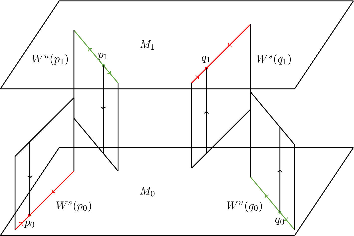
 (see Figure 1). We actually prove that for
$F\in \mathrm {PHI}^1(M)$
 , if F is boundary interconnected, then there exists an open neighborhood
$\mathcal {U}\subseteq \mathrm {PHI}^1(M)$
 of F such that every
$G\in \mathcal {U}\cap \mathrm {PHI}^2(M)$
 is topologically transitive, see Corollary 3.7. This kind of robust transitivity is exactly similar to the concept of stable ergodicity: It relies on a
$C^1$
 -robust structure provided by a
$C^2$
 partially hyperbolic diffeomorphism, which exactly corresponds to the role of the absolute continuity in the stably ergodic issue with Hopf’s argument.
Boundary interconnection (color online).

Figure 1 Long description
The diagram consists of two horizontal parallel planes labeled M sub 1 at the top and M sub 0 at the bottom.
On the top plane M sub 1:
- A green diagonal line on the left contains point p sub 1, with arrows pointing away from the point. It is labeled W super u (p sub 1).
- A red diagonal line on the right contains point q sub 1, with arrows pointing toward the point. It is labeled W super s (q sub 1).
On the bottom plane M sub 0:
- A red diagonal line on the left contains point p sub 0, with arrows pointing toward the point. It is labeled W super s (p sub 0).
- A green diagonal line on the right contains point q sub 0, with arrows pointing away from the point. It is labeled W super u (q sub 0).
Interconnections:
- Vertical black lines with directional arrows connect the points between planes.
- A line with a downward arrow connects p sub 1 to the red line on M sub 0.
- A line with an upward arrow connects q sub 0 to the red line on M sub 1.
- Rectangular and trapezoidal frames represent the manifold boundaries bridging the space between the two planes, showing how the stable and unstable manifolds of the points p and q intersect or relate across the boundary.
Remark 1.7. The geometric and algebraic structure of M is crucial for Theorem A. In fact, the conclusion does not hold when
$F_i: M_i \to M_i$
 is a general uniformly hyperbolic system, rather than an Anosov diffeomorphism on a nilmanifold. For example, let
${\sigma : \Sigma \to \Sigma }$
 be the classical horseshoe, where
$\Sigma = \{0,1\}^{\mathbb {Z}}$
 and
$\sigma (x)_i = x_{i + 1}$
 . Assume that
${\Phi : [0,1] \to [0,1]}$
 is a smooth diffeomorphism with exactly two fixed points, a source at
$1$
 and a sink at
$0$
 . Assume further that
$\Phi '$
 is dominated by the hyperbolicity of
$\sigma $
 , and consider the partially hyperbolic system
$F: \Sigma \times [0,1] \to \Sigma \times [0,1]$
 ,
$F(x,t) = (\sigma (x), \Phi _x(t))$
 , where
$\Phi _x = \Phi $
 when
$x_0 = 0$
 and
$\Phi _x = \Phi ^{-1}$
 when
$x_0 = 1$
 . Then, F is boundary interconnected but not topologically transitive. In fact, choose two fixed points
$p = (0),\ q = (1)$
 of
$\sigma $
 , then
$p_0 :=(p,0)$
 ,
$p_1 := (p,1)$
 ,
$q_0 := (q,0)$
 , and
$q_1 := (q,1)$
 satisfy the property that we need for boundary interconnection. However, if we take open intervals
$U,\ V\subseteq (0,\ 1)$
 such that
$\Phi ^n(U)\cap V = \varnothing $
 for any
$n\in \mathbb {Z}$
 , then
$\Sigma \times \bigcup _{n\in \mathbb {Z}}\Phi ^n(U)$
 and
$\Sigma \times \bigcup _{n\in \mathbb {Z}}\Phi ^n(V)$
 are disjoint F-invariant open subsets, and hence F is not topologically transitive.
1.2 Robustly intermingled basins
The phenomenon of intermingled basins was originally investigated by Kan [Reference KanKan94], and summarized by Bonatti et al [Reference Bonatti, Díaz and VianaBDV05]. In such a system, there are two Sinai–Ruelle–Bowen (SRB; physical) measures, both of whose basins admit positive volume in every non-empty open subset. Some of these examples are topologically transitive or even topologically mixing [Reference Gan and ShiGS19, Reference XiaXia24], indicating the significant difference between the topological and measure-theoretical notions of indecomposability. Moreover, Kan’s intermingled basins are robust [Reference Kleptsyn and SaltykovKS11].
This type of construction continues to be a source of interesting research and has been especially studied in the aspect of intermingled basins [Reference Melbourne and WindsorMW05, Reference Dolgopyat, Viana and YangDVY16, Reference Bonatti and PotrieBP18, Reference Ures and VásquezUV18]. There is also a family of topologically transitive diffeomorphisms constructed by inserting a blender and embedding into a boundaryless manifold [Reference Cheng, Gan and ShiCGS18]. More recently, there have been some advances focusing on the number of measures of maximal entropy for systems related to this type of construction [Reference Núñez-Madariaga, Ramírez and VásquezNnRV21, Reference Rocha and TahzibiRT22].
Specifically, we describe the phenomenon of intermingled basins in the setting of partially hyperbolic diffeomorphisms with interval central leaves.
Given
$F\in \mathrm {PHI}^k(M)\ (k \geq 2)$
 , for
$i = 0,1$
 , there exists a unique SRB measure
$\mu _i$
 on
$M_i$
 for
$F_i$
 , since
$F_i$
 is an Anosov diffeomorphism on a nilmanifold
$M_i$
 and therefore topologically transitive. We call them the boundary SRB measures of F.
Denote by
$\mathrm {PHI}_-^k(M)\ (k \geq 2)$
 the collection of diffeomorphisms
$F\in \mathrm {PHI}^k(M)$
 that are mostly contracting along the center direction on each boundary, that is, both of the boundary SRB measures
$\mu _i\ (i = 0,1)$
 admit negative central Lyapunov exponents, in the sense that

Note that
$\mathrm {PHI}^k_-(M)$
 is open in
$\mathrm {PHI}^k(M)$
 , and for
$F\in \mathrm {PHI}^k_-(M)$
 ,
$\mu _i\ (i = 0,1)$
 is not only an SRB measure for
$F_i$
 , but also a physical measure for F.
Definition 1.8. We say that
$F\in \mathrm {PHI}_-^k(M)$
 admits intermingled basins if the basins of its boundary SRB (physical) measures,
$B(\mu _0)$
 and
$B(\mu _1)$
 , both admit positive volume inside any non-empty open subset of M, and their union has full volume. Further, we say that F admits
$C^k$
 -robustly intermingled basins if there exists an open neighborhood
$\mathcal {U}\subseteq \mathrm {PHI}_-^k(M)$
 of F such that every
$G\in \mathcal {U}$
 admits intermingled basins.
An interesting result of Ures and Vásquez [Reference Ures and VásquezUV18] showed that the phenomenon of robustly intermingled basins does not appear on
$\mathbb {T}^3$
 , indicating the particularity of manifolds with a boundary.
In this paper, we also obtain the characterization of robustly intermingled basins for partially hyperbolic diffeomorphisms with interval central leaves that are mostly contracting along the center direction on each boundary.
Theorem B. For
$F\in \mathrm {PHI}_-^k(M)\ (k \geq 2)$
 , the following statements are equivalent:
-
(1) F admits $C^k$
-robustly intermingled basins; -
(2) F is $C^k$
-robustly transitive; -
(3) F is boundary interconnected.


As an application of Theorems A and B, consider the skew-product system

where
$A\in \mathrm {Aut}(\mathbb {T}^d)$
 is a hyperbolic toral automorphism with hyperbolic splitting
$L^s\oplus L^u$
 and
$\varphi (x, t): \mathbb {T}^d\times [0, 1] \to [0, 1]$
 is a
$C^k\ (k \geq 2)$
 map such that
$\varphi (x, \cdot ) \in \mathrm {Diff}_\partial ^k([0, 1])$
 for each
$x\in \mathbb {T}^d$
 . Assume that

Then,
$A_\varphi \in \mathrm {PHI}^k(\mathbb {T}^d\times [0, 1])$
 . For convenience, we denote the iterations of
$A_\varphi $
 by

Following the definition proposed by Bonatti et al [Reference Bonatti, Díaz and VianaBDV05, Ch. 11.1.1], we say that
$A_\varphi $
 is a Kan-type skew-product system if there exist two periodic points p and q of
$A\in \mathrm {Aut}(\mathbb {T}^d)$
 with periods
$\pi (p)$
 and
$\pi (q)$
 , such that
$\varphi _p^{\pi (p)}$
 has exactly two fixed points, a source at
$(p,1)$
 and a sink at
$(p,0)$
 ;
$\varphi _q^{\pi (q)}$
 also has exactly two fixed points, a source at
$(q,0)$
 and a sink at
$(q,1)$
 . Further, we say that
$A_\varphi $
 is mostly contracting if

By Theorem A, Kan-type skew-product systems are
$C^k$
 -robustly transitive. By Theorem B, mostly contracting Kan-type skew product systems admit
$C^k$
 -robustly intermingled basins for which the boundary SRB measures coincide with the Lebesgue measure restricted to each boundary component.
1.3 Organization
This paper is organized as follows. In §2, we introduce some basic definitions and results. In §3, we establish topological transitivity from boundary interconnection (Theorem 3.1), which exactly shows
$C^2$
 -robust transitivity in Theorem A. Then, we complete the proof of Theorem A in §4, showing that
$C^\infty $
 -robust transitivity implies boundary interconnection. In §5, we prove Theorem B by establishing the equivalence between robustly intermingled basins and boundary interconnection.
2 Preliminaries
2.1 Partially hyperbolic diffeomorphisms with interval central leaves
As defined in §1, M is a thickened nilmanifold,
$\mathrm {Diff}_\partial ^k(M)$
 is the collection of
$C^k$
 diffeomorphisms on M preserving each boundary
$M_0$
 and
$M_1$
 ,
$\mathrm {PHI}^k(M)$
 is the collection of partially hyperbolic diffeomorphisms in
$\mathrm {Diff}_\partial ^k(M)$
 with interval central leaves, and
$\mathrm {PHI}_-^k(M)$
 is the collection of diffeomorphisms in
$\mathrm {PHI}^k(M)$
 whose boundary SRB measures admit negative central Lyapunov exponents.
For
$F\in \mathrm {PHI}^2(M)$
 , the dynamical foliations
$\mathcal {F}^\sigma $
 are Hölder continuous with
$C^{1+}$
 leaves, for
$\sigma = s,c,u,cs,cu$
 . A subset of M is
$\sigma $
 -saturated if it is a union of
$\sigma $
 -leaves. There is a well-known result on the regularity of holonomy maps in [Reference Pugh, Shub and WilkinsonPSW97], which we state in our setting as follows. Note that
$F\in \mathrm {PHI}^2(M)$
 is dynamically coherent and center bunched, in the sense that for any
$x\in M$
 ,

Lemma 2.1. [Reference Pugh, Shub and WilkinsonPSW97, Theorem B]
For
$F\in \mathrm {PHI}^2(M)$
 , the holonomy map along the stable foliation (respectively the unstable foliation) restricted to a center-stable leaf (respectively a center-unstable leaf) is a
$C^1$
 diffeomorphism. Moreover, the derivative of the holonomy map is uniformly continuous with respect to the base points.
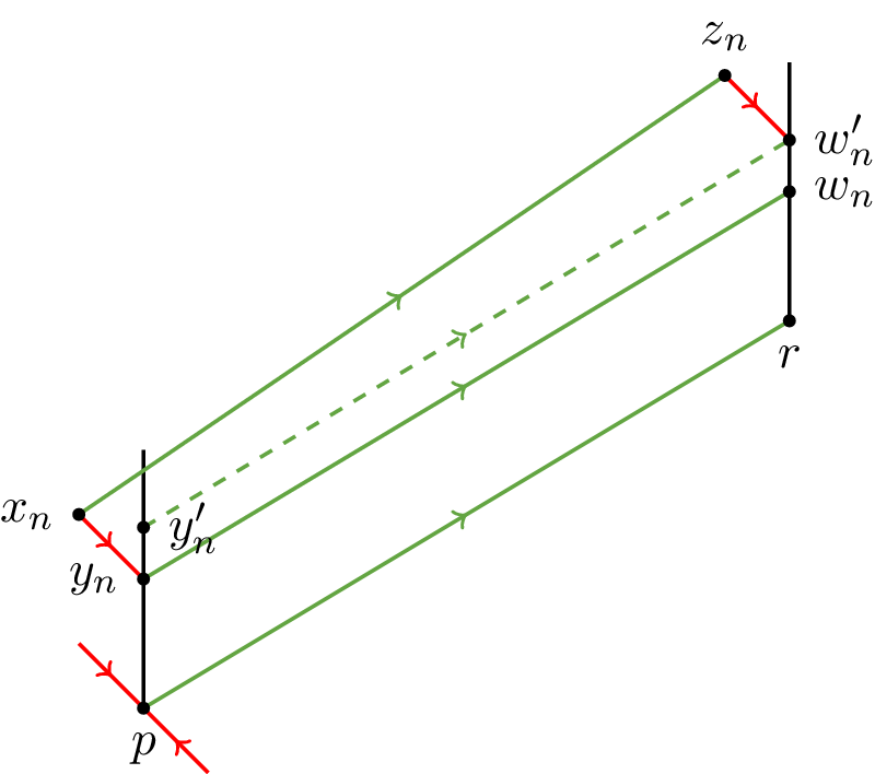
Central twist (color online).

The following result on the estimate of central twist is useful in our proof.
Lemma 2.2. Assume that
$F\in \mathrm {PHI}^2(M)$
 and
$p\in M_0$
 is a fixed point of
$F_0$
 with
${\unicode{x3bb} ^c(p) < 0}$
 . Fix
$r\in \mathcal {F}^u(p)$
 and let
$\mathrm {Hol}_p^r: \mathcal {F}^{cs}_{\mathrm {loc}}(p) \to \mathcal {F}^{cs}_{\mathrm {loc}}(r)$
 be the holonomy map along the unstable foliation. For
$x_0\in \mathcal {F}^{cs}_{\mathrm {loc}}(p)$
 , denote
$x_n = F^n(x_0)$
 for every
$n\in \mathbb {N}$
 and define

Then, we have the following estimate:

Here,
$C\geq 1$
 is a constant depending on p and r, and

where

Proof. Take
$y^{\prime }_n := (\mathrm {Hol}_p^r)^{-1}(w^{\prime }_n)$
 , see Figure 2. By Lemma 2.1, the holonomy map
$\mathrm {Hol}_p^r$
 restricted to
$\mathcal {F}^c_{\mathrm {loc}}(p)$
 is a
$C^1$
 diffeomorphism. Hence, it suffices to estimate
$d_c(y^{\prime }_n,\ y_n)$
 . First, note that

when
$n - N$
 is sufficiently large. Therefore, there exists a constant
$C\geq 1$
 such that

Now, let
$-N\unicode{x3bb} ^u(p) \approx (n - N)\unicode{x3bb} ^s(p)$
 , then we take

It follows that when n is sufficiently large, we have

where

This completes the proof of Lemma 2.2.
2.2 Asymptotically rational independence of Birkhoff sums
Here, we collect some results related to Birkhoff sums in the uniformly hyperbolic setting.
First, there is a concept of asymptotically rational independence introduced in [Reference Gan and ShiGS19]. For real numbers
$a,b\in \mathbb {R}$
 , define

Particularly, this notation
$(a,\ b)$
 coincides with
$\gcd (a,b)$
 when
$a,b\in \mathbb {Z}$
 . Recall that two real numbers
$a,b$
 are rationally independent if and only if
$(a,\ b) = 0$
 . Inspired by this fact, the asymptotically rational independence is defined as follows.
Definition 2.3. Let
$b\in \mathbb {R}$
 . A sequence
$\{a_m\}\subseteq \mathbb {R}$
 is asymptotically rationally independent of b if
$(a_m,\ b) \to 0$
 as
$m\to +\infty $
 .
To understand the asymptotically rational independence, we state the following results.
Lemma 2.4. If
$a,b\in \mathbb {R}$
 and
$b\neq 0$
 , then
$(a,\ b) < \varepsilon $
 for some
$\varepsilon> 0$
 if and only if each orbit of
$T_a(x) := x + a\ (\mathrm {mod}\ b\mathbb {Z})$
 is
$\varepsilon $
 -dense in
$\mathbb {R}/(b\mathbb {Z})$
 . In particular, if
$(a,\ b)> 0$
 , then
$(a,\ b)=|b|/q$
 for the reduced fraction
$a/b=p/q$
 with
$p\in \mathbb {Z},\ q\in \mathbb {N},\ (p,\ q) = 1$
 .
Proof. The conclusion follows directly from the definition of
$(a,\ b)$
 .
Lemma 2.5. If
$a_1,a_2,b\in \mathbb {R}$
 and
$b\neq 0$
 , then
$0 < |a_1 - a_2| < \varepsilon \ (\mathrm {mod}\ b\mathbb {Z})$
 implies that there exists
$a\in \{a_1,a_2\}$
 such that
$(a,\ b) < {\sqrt {|b|\,\varepsilon }}$
 .
Proof. Given
$b\neq 0$
 , notice that

is a finite set, in which for any
$a_1,a_2$
 with
$a_1\neq a_2 \ {(\mathrm {mod}\ b\mathbb {Z})}$
 , we have
$|a_1 - a_2| \geq \varepsilon \ (\mathrm {mod}\ b\mathbb {Z})$
 . In fact, taking the reduced fractions

we have
$p_1q_2-p_2q_1-kq_1q_2\neq 0$
 for any
$k\in \mathbb {Z}$
 ; hence,

and then

Therefore,
$0 < |a_1 - a_2| < \varepsilon \ (\mathrm {mod}\ b\mathbb {Z})$
 implies that at least one of them does not belong to the finite set.
Now, we introduce the Birkhoff sums. Let
$A: N \to N$
 be an Anosov diffeomorphism on a nilmanifold and
$\varphi : N \to \mathbb {R}$
 be a Hölder continuous function. Denote by

the Birkhoff sum of the function
$\varphi $
 along a periodic orbit of
$p\in \mathrm {Per}(A)$
 with period
$\pi (p)$
 .
The following positive Livšic theorem (see [Reference Lopes and ThieullenLT03]) or Mañé–Conze–Guivarc’h–Bousch lemma (see [Reference BouschBou01, Reference BouschBou11]) is a classical method to obtain the information of the whole space from that of periodic orbits.
Lemma 2.6. (Positive Livšic theorem)
Let
$A: N \to N$
 be an Anosov diffeomorphism on a nilmanifold and
$\varphi : N \to \mathbb {R}$
 be a Hölder continuous function. If

then there exists a Hölder continuous function
$\psi : N \to \mathbb {R}$
 such that
$\varphi \geq \psi - \psi \circ A$
 .
For
$F\in \mathrm {PHI}^1(M)$
 , we have an Anosov diffeomorphism
$F_0: M_0 \to M_0$
 . Define

Then, for a periodic point
$p\in \mathrm {Per}(F_0)$
 with period
$\pi (p)$
 , the corresponding Birkhoff sum
$S_\varphi F_0(p)$
 is exactly the total central Lyapunov exponent
$\pi (p)\unicode{x3bb} ^c(p)$
 . Hence, the Birkhoff sum is regarded as an observation function involving the information of central Lyapunov exponents.
In particular, we have the following corollary of Lemma 2.6.
Corollary 2.7. For
$F\in \mathrm {PHI}^1(M)$
 , if
$\unicode{x3bb} ^c(p) \leq 0$
 for every
$p\in \mathrm {Per}(F_0)$
 , then
$\unicode{x3bb} ^c(x) \leq 0$
 whenever
$\unicode{x3bb} ^c(x)$
 exists.
There is the following rigidity result on the distribution of all Birkhoff sums.
Lemma 2.8. [Reference Gan, Shi and XiaGSX22, Theorem 1.1]
Let
$A: N \to N$
 be an Anosov diffeomorphism on a nilmanifold and
$\varphi : N \to \mathbb {R}$
 be a Hölder continuous function. If there are two periodic points
$p_0,q_0\in \mathrm {Per}(A)$
 satisfying

then the set
$\{S_\varphi A(p): p\in \mathrm {Per}(A)\}$
 is dense in
$\mathbb {R}$
 .
2.3 Analysis in the one-dimensional dynamics
The following quantitative result is prepared for analyzing the one-dimensional center dynamics connected by a holonomy map. The proof is technical and may be skipped on a first reading.
Proposition 2.9. Let
$f,g\in \mathrm {Diff}_\partial ^{1+}([0,1])$
 be diffeomorphisms with exactly two fixed points
$0,1$
 , where
$0$
 is a hyperbolic sink; and
$h\in \mathrm {Diff}_\partial ^1([0,1])$
 . Then, there exist
$\varepsilon _0> 0$
 and an increasing function
$L(\varepsilon ): (0,\varepsilon _0) \to (0,1)$
 satisfying
$L(x)\to 0$
 as
$x\to 0^+$
 and depending on
$\beta := g'(0)$
 , such that the following conclusion holds. If
$\alpha := f'(0)$
 satisfies

then for any two closed intervals
$I,J \subseteq (0,1)$
 with
$|J|> L(\varepsilon )$
 , there exist two strictly increasing subsequences
$\{k_n\},\{l_n\}$
 of
$\mathbb {N}$
 such that

Moreover, there exists a constant
$c> 0$
 such that

Proof. First, we have the following expansions:

For any
$k,l\in \mathbb {N}$
 , we also have

Hence, for any
$\varepsilon> 0$
 , we can take
$0 < \delta < 1$
 sufficiently small such that

Since
$(\ln \alpha ,\ \ln \beta ) < \varepsilon $
 , there exist
$K^*$
 ,
$L^*\in \mathbb {Z}^+$
 depending on
$\beta $
 such that for any
${\eta \in (\beta ^2, 1)}$
 , there exist
$1\leq K\leq K^*$
 ,
$1\leq L\leq L^*$
 such that

Therefore, by taking
$\delta $
 smaller, we may further require that

It follows that

For
$x\in [0, \delta ]$
 , define
$I_x := (g(h(x)),\, h(x)]$
 . Then, we have the following conclusion.
Claim 2.10. For any
$x\in [0,\delta ]$
 and any closed interval
$J\subseteq I_x$
 with

there exist
$1\leq K \leq K^*$
 and
$1\leq L \leq L^*$
 such that

Proof of Claim 2.10.
Note that
$|I_x|> (1 - \beta - \varepsilon )h(x)$
 and, hence,
$|J|> 3\varepsilon h(x)$
 . It follows that there exists
$\eta \in (\beta ^2, e^{-\varepsilon })$
 such that

because the error
$((e^\varepsilon - 1)\eta + 2\varepsilon )h(x) < 3\varepsilon h(x)$
 . It follows that there exist
$1\leq K \leq K^*$
 ,
$1\leq L \leq L^*$
 such that

This completes the proof of Claim 2.10.
For any point
$y\in (0,1)$
 and closed interval
$J\subseteq (0,1)$
 , define the fundamental domains
$\Omega _i := (g^{i + 1}(y),\, g^i(y)]$
 , and denote
$J^* := \bigcup _{i\in \mathbb {Z}}g^i(J)$
 and
$J_i := J^*\cap \Omega _i$
 for any
$i\in \mathbb {Z}$
 . Then, we have the following conclusion.
Claim 2.11. There exists a constant
$0 < \rho < 1$
 such that

In particular, there exists a constant
$c> 0$
 such that
$|g^i(J)| \geq c\beta ^i\ \text {for all } i\in \mathbb {N}$
 .
Proof of Claim 2.11.
Note that
$J_i$
 does not change when we replace J by
$J_0$
 . Since
$J_0$
 has at most two components, by considering each component, we may assume at first that
$J = [a,b]\subseteq \overline {\Omega }_0$
 . Without loss of generality, assume that
$j> i$
 . Then, we have

where
$\xi _1\in J_i$
 and
$\xi _2\in \Omega _i$
 , and hence,

Here,
$0 < \theta < 1$
 is the Hölder exponent of
$\ln g'$
 in
$[0,h(\delta )]$
 and
$C \geq 1$
 is a constant depending on g. Therefore, we can take

This completes the proof of Claim 2.11.
Consider the family of fundamental domains

Claim 2.12. There exist
$\varepsilon _0> 0$
 and an increasing function
$G: (0,\varepsilon _0) \to (0, 1)$
 satisfying
$G(x)\to 0$
 as
$x\to 0^+$
 and
$r = r(s, t): D_0\times D_0 \to \{-1,\, 0,\, 1\}$
 such that

where
$J_s(\varepsilon ) := [s - G(\varepsilon ),\, s]$
 .
Proof of Claim 2.12.
Fix any
$s\in D_0$
 . Considering the relative position of s and
$I_t$
 , we need the following sufficient conditions:

Finally, we take

One can check that
$G(\cdot )$
 is increasing and
$G(x)\to 0$
 as
$x\to 0^+$
 . Note that we take
$\varepsilon _0> 0$
 sufficiently small so that when
$0 < \varepsilon < \varepsilon _0$
 , the above discussions make sense.
Now, we prove Proposition 2.9. Define

Note that we take
$\varepsilon _0> 0$
 sufficiently small so that when
$0 < \varepsilon < \varepsilon _0$
 , the function
$L(\cdot )$
 is well defined. One can check that
$L(\cdot )$
 is increasing and
$L(x)\to 0$
 as
$x\to 0^+$
 .
We claim that
$|J|> 3L(\varepsilon )$
 will be sufficient.
In fact, for any point
$x\in (0, 1)$
 and closed interval
$J\subseteq (0, 1)$
 with
$|J|> L(\varepsilon )$
 , there exist
$k^*\in \mathbb {N}$
 and
$l^*\in \mathbb {Z}$
 such that
$f^{k^*}(x)\in (0, \delta )$
 and
$g^{l^*}(J) = [s - |g^{l^*}(J)|,\, s]$
 for some
$s\in D_0$
 . Moreover,

By Claim 2.12, we have

where
$r\in \{-1,\, 0,\, 1\}$
 depends on J and
$t\in D_0$
 . In particular, for each
$n\in \mathbb {N}$
 large enough, consider the fundamental domain

and let
$\widehat {l}_n\in \mathbb {N}$
 be the unique integer such that

Then, we have

where
$r_n\in \{-1,\, 0,\, 1\}$
 depends on x and J.
By Claim 2.11, we have

By Claim 2.10, there exist
$1\leq K_n \leq K^*$
 and
$1\leq L_n \leq L^*$
 such that

Finally, we take
$k_n = n + k^* + K_n$
 and
$l_n = \widehat {l}_n + l^* + r_n + L_n$
 , and then we have

Since
$k_n \to +\infty $
 and
$l_n \to +\infty $
 as
$n \to +\infty $
 , by taking a subsequence if necessary, we can require that the sequences
$\{k_n\}$
 and
$\{l_n\}$
 are positive and strictly increasing.
It follows that for any two closed intervals
$I,J\subseteq (0, 1)$
 with
$|J|> 3L(\varepsilon )$
 , there exist strictly increasing subsequences
$\{k_n\}$
 ,
$\{l_n\}$
 of
$\mathbb {N}$
 such that

where
$J'$
 is the middle third of J. Then, we have the following two cases.
Case 1.
$h\circ f^{k_n}(I)$
 is totally contained in
$g^{l_n}(J)$
 . Applying Claim 2.11 to f, we have

for some constant
$c> 0$
 .
Case 2.
$h\circ f^{k_n}(I)$
 is not totally contained in
$g^{l_n}(J)$
 . Assume that
$J = [a,b]$
 and
${J' = [a',b']}$
 , then
$h\circ f^{k_n}(I)$
 contains
$g^{l_n}([a, a'])$
 or
$g^{l_n}([b',b])$
 . Applying Claim 2.11, we have

for some constant
$c> 0$
 .
Recall that by the choice of
$\widehat {l}_n$
 , we have

Hence, there exists a constant
$C \geq 1$
 such that

We conclude that

As a result, there exists a constant
$c> 0$
 such that

This completes the proof of Proposition 2.9.
3 Boundary interconnection implies topological transitivity
In this section, we prove that boundary interconnection implies topological transitivity.
Theorem 3.1. Assume that
$F\in \mathrm {PHI}^2(M)$
 . If F is boundary interconnected, then F is topologically transitive.
First, we characterize the stable set of a periodic point with a uniformly contracting center.
Lemma 3.2. Let
$p\in \mathrm {Per}(F_0)$
 be a periodic point with period
$\pi (p)$
 and
$\unicode{x3bb} ^c(p) < 0$
 . Assume that
$\gamma _p: [0, 1] \to \mathcal {F}^c(p)$
 is a
$C^{1+}$
 parameterization of the central leaf of p with
$\gamma _p(0) = p$
 . Then, there exists
$0 < s_p \leq 1$
 satisfying

In particular, define
$\ell _p:[0,1]\to [0,s_p]$
 and
$\ell _p(t):=s_p t$
 , then
$\gamma _p^s := \gamma _p\circ {\ell _p} : [0, 1] \to \bar {I}_p^c$
 is a
$C^{1+}$
 parameterization, and

is a diffeomorphism with exactly two fixed points
$0,1$
 , where
$0$
 is a hyperbolic sink.
Proof of Lemma 3.2.
Notice that
$f_p := (\gamma _p)^{-1}\circ F^{\pi (p)}\circ \gamma _p \in \mathrm {Diff}_\partial ^{1+}([0, 1])$
 . Since
$\unicode{x3bb} ^c(p) < 0$
 , we have
$0 < f^{\prime }_p(0) < 1$
 and, therefore,
$f_p$
 has a smallest positive fixed point
$0 < s_p \leq 1$
 . It follows that
${\ell _p}^{-1}\circ f_p\circ {\ell _p}\in \mathrm {Diff}_\partial ^{1+}([0, 1])$
 is a diffeomorphism with exactly two fixed points
$0,1$
 , where
$0$
 is a hyperbolic sink.
By the above argument,
$I_p^c := W^s(p)\cap \mathcal {F}^c(p) = \gamma _p([0, s_p))$
 . Therefore, we have

Now, take
$y\in W^s({p})$
 . Then, we have
$\pi _0(y)\in \mathcal {F}^s(\pi _0({p}))$
 . Recall that
$\pi _0: M \to M_0$
 is the natural projection along central leaves. It follows that
$y\in \mathcal {F}^{cs}({p})$
 . Assume that
$y\in \mathcal {F}^s(z)$
 for some
$z\in \mathcal {F}^c({p})$
 . Then,
$z\in W^s(p)$
 and, hence,
$z\in I_p^c$
 since
$W^s(p)$
 is s-saturated. This completes the proof of Lemma 3.2.
Note that similar conclusions hold for periodic points of both
$F_0$
 and
$F_1$
 : The stable set (respectively unstable set) is characterized by the uniformly contracting center (respectively uniformly expanding center) when the central Lyapunov exponent is negative (respectively positive). For simplicity, we omit the statement for the other case.
Now, we prove Theorem 3.1.
Proof of Theorem 3.1.
It suffices to show that for any two non-empty open subsets
${U, V\subseteq M}$
 , there exists
$N\in \mathbb {N}$
 such that
$F^N(U)\cap V\neq \varnothing $
 . Equivalently, we only need to show that
$U^*\cap V^*\neq \varnothing $
 , where

Note that
$F(U^*)\subseteq U^*$
 , hence,
$U^*$
 is u-saturated;
$F^{-1}(V^*)\subseteq V^*$
 ; and
$V^*$
 is s-saturated.
Since F is boundary interconnected, there exist two pairs of periodic points
$p_i,q_i\in M_i$
 such that

Without loss of generality, we assume that the periodic points
$p_i$
 and
$q_i$
 are fixed points. Define
$\varphi : M \to \mathbb {R}$
 by

Then,
$\varphi $
 is Hölder continuous, and there exist constants
$C_\varphi \geq 1$
 and
$0 < \theta < 1$
 such that

Recall that we denote by

the Birkhoff sum of the function
$\varphi $
 for
$p\in \mathrm {Per}(F_0)$
 with period
$\pi (p)$
 . As a result,

Generate new periodic points for asymptotically rational independence. Now, compared with the results in [Reference XiaXia24], we do not know whether
$S_\varphi F_0(p_0)$
 and
$S_\varphi F_0(q_0)$
 are rationally independent. Therefore, we need the following asymptotic version.
Claim 3.3. There exists a sequence of periodic points
$\{p_{0,m}\}\subseteq \mathrm {Per}(F_0)$
 such that

Proof of Claim 3.3.
If
$S_\varphi F_0(p_0)$
 and
$S_\varphi F_0(q_0)$
 are indeed rationally independent, then we just take
$p_{0,m} = p_0$
 for any
$m\in \mathbb {N}$
 . Now, we assume that
$S_\varphi F_0(p_0)$
 and
$S_\varphi F_0(q_0)$
 are rationally dependent. By Lemma 2.8, the set
$\{S_\varphi F_0(p): p\in \mathrm {Per}(F_0)\}$
 is dense in
$\mathbb {R}$
 . Therefore, there exists a sequence of periodic points
$\{\bar {p}_{0,m}\} \subseteq \mathrm {Per}(F_0)$
 such that

For fixed
$m\in \mathbb {N}$
 , we construct
$p_{0,m}$
 from
$\bar {p}_{0,m}$
 by the shadowing property.
An Anosov diffeomorphism on a nilmanifold
$M_0$
 ,
$F_0$
 is topologically transitive. Hence,
$\bar {p}_{0,m}$
 and
$p_0$
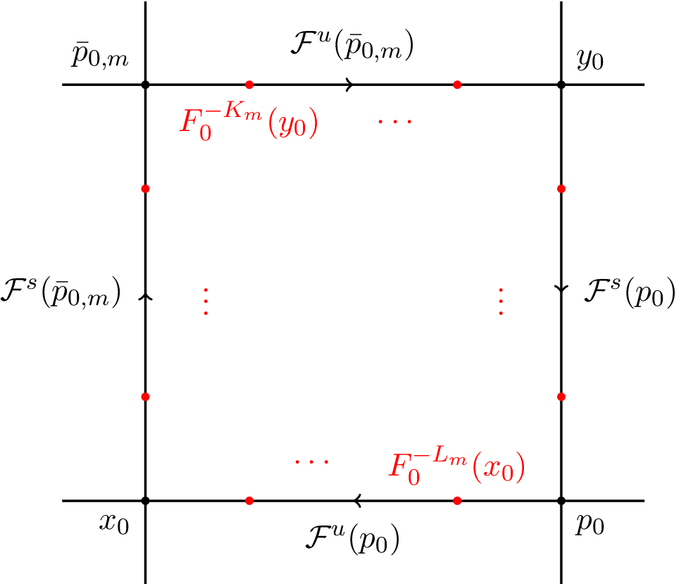
 are homoclinically related, and there are points
$x_0, y_0\in M_0$
 with

see Figure 3. For simplicity, we omit the picture of the other points in
$\mathrm {Orb}(\bar {p}_{0,m})$
 .
Periodic pseudo-orbit (color online).

We then consider the following pseudo-orbit segment:

Here,
$K_m,L_m\in \mathbb {N}$
 are large multiples of
$\pi (\bar {p}_{0,m})$
 to be decided. The sum of
$\varphi $
 over
$\mathcal {P}^{\prime }_m$
 is

Since
$F_0$
 is uniformly contracting (respectively expanding) in stable (respectively unstable) manifolds and
$\varphi $
 is Hölder continuous, we have the following convergent series:

As a result, given a sequence of positive numbers
$\bar {\varepsilon }_m \to 0$
 , there exist
$K_m^0, L_m^0\in \mathbb {N}$
 being multiples of
$\pi (\bar {p}_{0,m})$
 such that when
$K_m \geq K_m^0$
 and
$L_m \geq L_m^0$
 , we have

However, by the classical exponential Anosov shadowing lemma, there are constants
${0 < \delta _0 < 1}$
 ,
$C_0 \geq 1$
 , and
$0 < \mu _0 < 1$
 such that for every
$0 < \delta < \delta _0$
 , every
$\delta $
 -pseudo-orbit
$\{x_i: i_A\leq i \leq i_B\}\ (i_A \leq 0 \leq i_B)$
 is exponentially shadowed by a periodic point p in the sense that

As a result, there exist
$K_m^1, L_m^1\in \mathbb {N}$
 such that when
$K_m \geq K_m^1$
 and
$L_m \geq L_m^1$
 ,
$\mathcal {P}^{\prime }_m$
 is a
$\delta _0\bar {\varepsilon }_m$
 -pseudo-orbit, exponentially shadowed by a periodic point
$p_{0,m}'\in \mathrm {Per}(F_0)$
 . In fact, it suffices to take
$K_m^1$
 and
$L_m^1$
 to be multiples of
$\pi (\bar {p}_{0,m})$
 and so large that

Now, we consider
$S_\varphi F_0(p_{0,m}')$
 , which is the sum of
$\varphi $
 over the orbit of
$p_{0,m}'$
 . Since
$\varphi $
 is Hölder continuous, the difference between
$S_\varphi F_0(p_{0,m}')$
 and
$S_\varphi (\mathcal {P}^{\prime }_m)$
 is controlled by

Combining (3.2) and (3.3), there exists a constant
$C \geq 1$
 such that

Here, we choose
$K_m {\kern-1pt}={\kern-1pt} \max \{K_m^0, K_m^1, m\pi (\bar {p}_{0,m})\}$
 and
${L_m {\kern-1pt}={\kern-1pt} \max \{L_m^0, L_m^1, m(K_m+|P|)\}}$
 so that the central Lyapunov exponent is also controlled:

In the same manner as above, we can make a slight modification on the choice of the pseudo-orbit segment. Precisely, we add the periodic orbit of
$\bar {p}_{0,m}$
 and consider the following pseudo-orbit segment:

Then, we have a periodic point
$p_{0,m}"\in \mathrm {Per}(F_0)$
 shadowing
$\mathcal {P}^{\prime \prime }_m$
 and satisfying a similar estimate as (3.4):

Moreover, we also have that

Finally, we choose
$p_{0,m} \in \{p_{0,m}',\, p_{0,m}"\}$
 so that
$(S_\varphi F_0(p_{0,m}),\ S_\varphi F_0(p_0)) \to 0$
 as
${m \to +\infty }$
 . In fact, combining (3.4) and (3.5), we have

Now, taking
$\bar {\varepsilon }_m$
 so small that
$2C\bar {\varepsilon }_m^\theta < {2^{-m}}$
 , then we have the following estimate by combining (3.1) and (3.6):

Taking further
$3\cdot 2^{-m}< |S_\varphi F_0(p_0)|$
 , then by Lemma 2.5, there exists
${p_{0,m} \in \{p_{0,m}', p_{0,m}"\}}$
 such that

Since
$S_\varphi F_0(p_0)$
 and
$S_\varphi F_0(q_0)$
 are rationally dependent, there exists a sequence of positive numbers
$\varepsilon _m \to 0^+$
 such that
$(S_\varphi F_0(p_{0,m}),\ S_\varphi F_0(q_0)) < \varepsilon _m$
 .
This completes the proof of Claim 3.3.
In fact, we can modify the choice of
$\{p_{0,m}\}$
 to obtain more information about the sequence.
Claim 3.4. By replacing the periodic point
$p_{0,m}$
 by some points in
$\mathrm {Orb}(p_{0,m})$
 and taking a subsequence, we may assume further that the sequence
$\{p_{0,m}\}$
 constructed in Claim 3.3 satisfies the following properties.
-
• Better Birkhoff average:
$$ \begin{align*} \frac{1}{k}\sum_{i = 0}^{k - 1}\ln\|DF|_{E^c(F_0^i(p_{0,m}))}\| \leq \frac{\unicode{x3bb}^c(p_0)}{3}\quad \text{for all } k\in\mathbb{N},\ \text{for all } m\in\mathbb{N}. \end{align*} $$
-
• Uniform size of contracting center: there exists $\eta _0> 0$
such that $$ \begin{align*} |I_{p_{0,m}}^c| \geq \eta_0\quad \text{for all } m\in\mathbb{N}. \end{align*} $$
-
• Convergence: there exists $r_0\in M_0$
such that
$p_{0,m}\to r_0$
as
$m \to +\infty $
.


Proof of Claim 3.4.
Since
$\unicode{x3bb} ^c(p_{0,m}) \to \unicode{x3bb} ^c(p_0) < 0$
 , by taking a subsequence, we assume that

By the classical Pliss lemma, for each
$m\in \mathbb {N}$
 , there exists a hyperbolic time
$n_m$
 such that

Hence, we can replace
$p_{0,m}$
 by
$F_0^{n_m}(p_{0,m})\in \mathrm {Orb}(p_{0,m})$
 . Since
$p_{0,m}$
 is a periodic point, this replacement does not influence the properties that we need in Claim 3.3.
Now, we show that the length of the contracting center
$I_{p_{0,m}}^c$
 has a positive lower bound with respect to
$m\in \mathbb {N}$
 . Since
$p_{0,m}$
 now admits a better Birkhoff average, there exists a maximal closed interval
$I_m$
 containing
$p_{0,m}$
 as an endpoint, lying in
$I_{p_{0,m}}^c$
 , satisfying

where

Then, for
$x,y\in I_m$
 , we have

Let
$\widetilde {p}_{0,m}$
 be the other endpoint of
$I_m$
 . Since
$I_m$
 is maximal, there exists
$1\leq k_m \leq \pi (p_{0,m})$
 such that

As a result,

It follows that
$p_{0,m}$
 has a uniform size of contracting center.
Finally, since
$M_0$
 is compact, we can take a subsequence to ensure that
$p_{0,m}\to r_0$
 for some
$r_0\in M_0$
 .
Show the density of the stable and unstable sets. Next, we show that the intersection of the stable and unstable sets implies their density.
Claim 3.5. The stable and unstable sets
$W^s(p_0),W^u(q_0),W^u(p_1),W^s(q_1)$
 are dense in M.
Proof of Claim 3.5.
For convenience, we define
$\widehat {p}_0 := \pi _1(p_0)$
 and
$\widehat {p}_1 := \pi _0(p_1)$
 . Recall that
$W^s(p_0)\pitchfork W^u(p_1)$
 contains a central interval. Assume that the interval lies in a central leaf with endpoints
$z_0\in M_0$
 and
$z_1\in M_1$
 , then there exists an open central interval
${J \subseteq \mathcal {F}^c(z_0)}$
 with an endpoint
$z_0$
 , lying in
$W^s(p_0)$
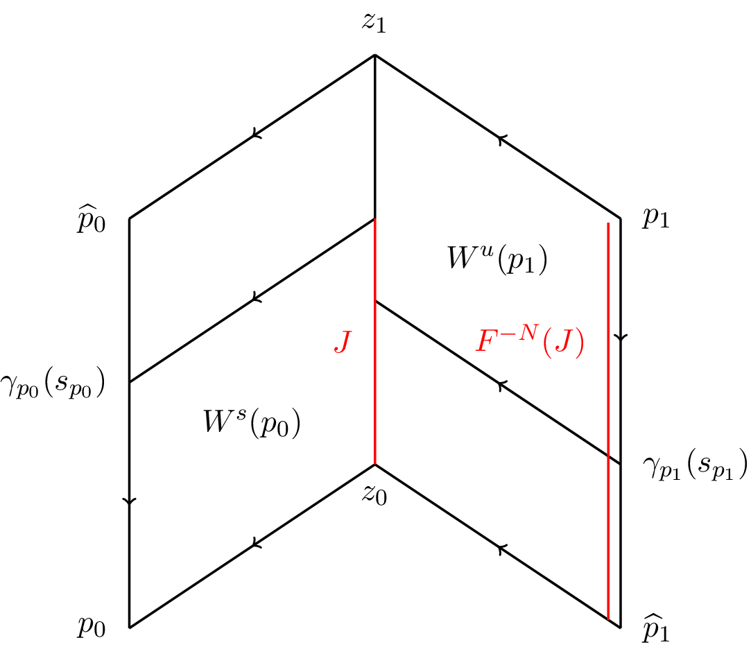
 and containing an interval in
$W^u(p_1)$
 , see Figure 4.
Density of
$W^s(p_0)$
 (color online).

Figure 4 Long description
The diagram consists of two rectangular planes meeting at a central vertical line.
Central Axis:
At the top of the central vertical line is the label z sub 1, and at the bottom is z sub 0. A red vertical segment on this axis is labeled J.
Left Plane:
The top-left corner is labeled p hat sub 0 and the bottom-left corner is p sub 0. A horizontal line with a left-pointing arrow bisects this plane, labeled gamma sub p sub 0 (s sub p sub 0). The region below this line is labeled W super s (p sub 0).
Right Plane:
The top-right corner is labeled p sub 1 and the bottom-right corner is p hat sub 1. A horizontal line with a left-pointing arrow bisects this plane, labeled gamma sub p sub 1 (s sub p sub 1). The region above this line is labeled W super u (p sub 1). A red vertical line segment on the far right edge is labeled F super minus N (J).
Directional Arrows:
Arrows on the outer boundaries point inward toward the central axis or downward along the vertical edges. Arrows on the horizontal bisecting lines point toward the left.
Now, consider
$F^{-N}(J)$
 . One of its endpoints is
$F_0^{-N}(z_0)$
 , which tends to
$\widehat {p}_1$
 ; the other endpoint tends to
$p_1$
 , since it lies in
$W^u(p_1)$
 . Moreover,
$F^{-N}(J)$
 is a central interval, and hence,
$F^{-N}(J)$
 tends to
$\mathcal {F}^c(p_1)$
 , in the sense that

Since
$F_0$
 is an Anosov diffeomorphism on a nilmanifold, the stable foliation restricted to
$M_0$
 is minimal, in the sense that each stable leaf is dense in
$M_0$
 . It follows that
$\mathcal {F}^{cs}$
 is minimal, because
$\mathcal {F}^{cs}(\cdot ) = \pi _0^{-1}(\mathcal {F}^s(\pi _0(\cdot )))$
 .
Now,
$\mathcal {F}^{cs}(p_1)$
 is dense in M, for any non-empty open subset
$U\subseteq M$
 , there exists
${x\in \mathcal {F}^c(p_1)}$
 such that
$\mathcal {F}^s(x)\cap U\neq \varnothing $
 . Note that

Therefore, there exists
$K = K(\varepsilon )\in \mathbb {N}$
 such that
$\mathcal {F}^s_\varepsilon ({F^K(x)})\cap F^K(U)\neq \varnothing $
 . Recall that
$F^{-N}(J)$
 tends to
$\mathcal {F}^c(p_1)$
 , hence, there exist
$N\in \mathbb {N}$
 and
$x'\in F^{-N}(J)$
 such that
$\mathcal {F}^s_\varepsilon ({F^K(x')})\cap F^K(U)\neq \varnothing $
 . Now, we have that
$\mathcal {F}^s(F^N({F^K(x')}))\cap F^{K + N}(U)\neq \varnothing $
 . Since
${F^N(F^K(x'))\in F^K(J)}\subseteq W^s(p_0)$
 , we conclude that

This shows the density of
$W^s(p_0)$
 . By the same argument,
$W^u(q_0), W^u(p_1)$
 , and
$W^s(q_1)$
 are also dense in M.
Move from
$p_0$
 to
$p_{0,m}$
 . We first show that the points in
$U^*$
 appear near the contracting central interval
$I_{p_{0,m}}^c$
 .
Since
$\unicode{x3bb} ^c(p_0) < 0$
 , we have

Therefore, by the density of
$W^s(p_0)$
 , we have

and hence, we can take

Moreover,
$U^*\cap \mathcal {F}^c(\widetilde {p}_0)$
 contains a closed central interval
$J_{\widetilde {p}_0}^c$
 , satisfying
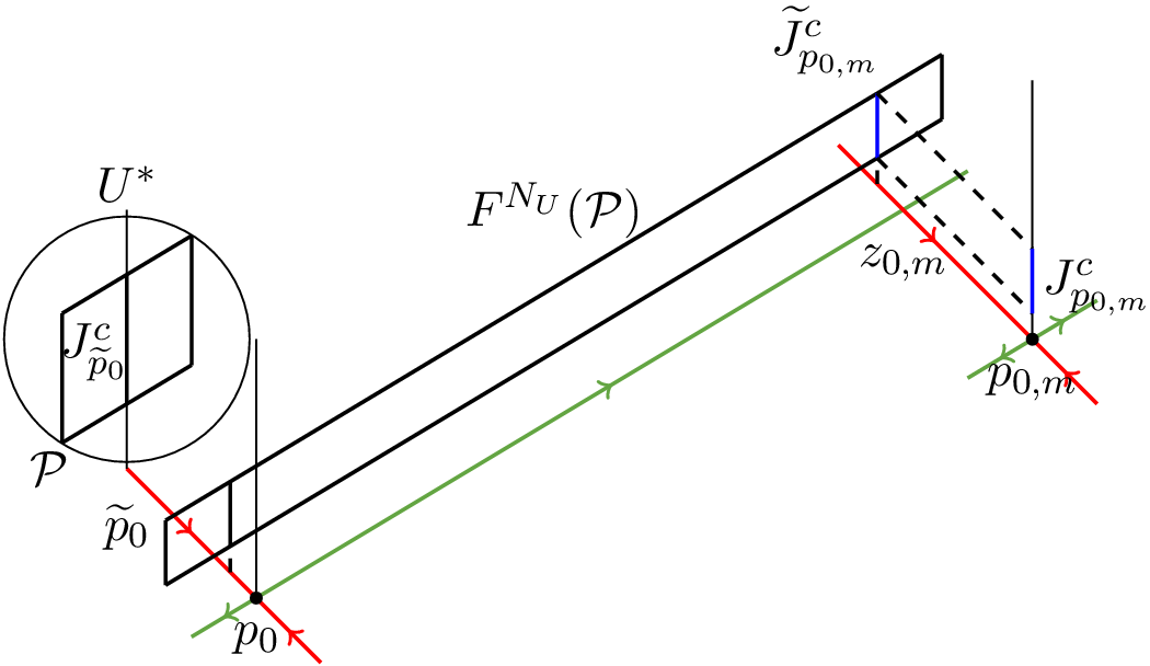
$\mathcal {P} := \mathcal {F}^u_{\mathrm {loc}}(J_{\widetilde {p}_0}^c)\subseteq U^*$
 , see Figure 5.
Holonomy map from
$p_0$
 to
$p_{0,m}$
 (color online).

Figure 5 Long description
The diagram depicts a geometric mapping between two regions.
* On the left, a circular region labeled U super asterisk contains a vertical rectangular plane labeled J sub p tilde sub 0 super c. A point p tilde sub 0 is located on a red line below this circle. Further down, a black dot labeled p sub 0 marks the intersection of the red line and a green line.
* A long, narrow rectangular strip labeled F super N sub U (P) extends diagonally from the left region toward the right.
* On the right side, the strip terminates at a vertical blue line segment labeled J tilde sub p sub 0 comma m super c.
* Below this, a red line and a green line intersect at a black dot labeled p sub 0 comma m.
* A vertical blue line segment above this intersection is labeled J sub p sub 0 comma m super c.
* Dashed lines connect the upper blue segment on the strip to the lower blue segment near the intersection point.
* A point on the red line between the strip and the final intersection is labeled z sub 0 comma m.
* Arrows on the red and green lines indicate the direction of flow toward the intersection points.
Similarly, since
$\unicode{x3bb} ^c(q_0)> 0$
 and
$W^u(q_0)$
 is dense in M, we have

and, hence, we can take

We can further require that
$V^*\cap \mathcal {F}^c(\widetilde {q}_0)$
 contains a closed central interval
$J_{\widetilde {q}_0}^c$
 satisfying
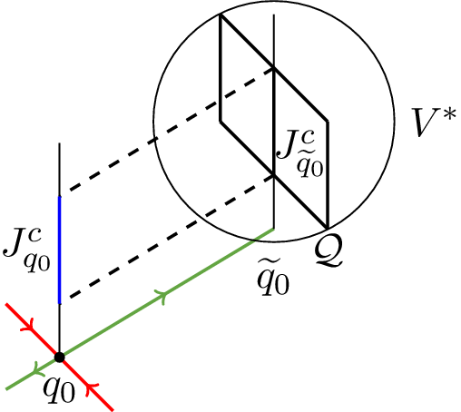
$\mathcal {Q} := \mathcal {F}^s_{\mathrm {loc}}(J_{\widetilde {q}_0}^c)\subseteq V^*$
 , see Figure 6.
Holonomy map near
$q_0$
 (color online).

Note that
$\mathcal {F}^u(p_0)$
 is dense in
$M_0$
 . Hence, we can choose
$z_{0,m}\in \mathcal {F}^u(p_0)\pitchfork \mathcal {F}^s_{\mathrm {loc}}(p_{0,m})$
 . Since
$p_{0,m}$
 converges, we may further assume that
$z_{0,m}$
 also converges.
In fact, by taking a subsequence, we assume that
$p_{0,m}$
 lies in the local
$su$
 -box of
$r_0$
 , then it suffices to ensure that
$\mathcal {F}^u(p_0)\pitchfork \mathcal {F}^s_{\mathrm {loc}}(r_0)\neq \varnothing $
 .
It follows that there exists
$N_U\in \mathbb {N}$
 independent of
$m\in \mathbb {N}$
 such that

In particular,
$F^{N_U}(\mathcal {P})\pitchfork \mathcal {F}^c(\mathcal {F}^s_{\mathrm {loc}}(p_{0,m}))$
 contains a central interval
$\widetilde {J}_{p_{0,m}}^c$
 , whose length has a positive lower bound with respect to
$m\in \mathbb {N}$
 .
Let
$J_{p_{0,m}}^c \subseteq \mathcal {F}^c(p_{0,m})$
 be the image of
$\widetilde {J}_{p_{0,m}}^c$
 under the holonomy map along the stable leaves, restricted to
$\mathcal {F}^{c}(\mathcal {F}^{s}_{\mathrm {loc}}(p_{0,m}))$
 . By Lemma 2.1, the length of
$J_{p_{0,m}}^c$
 also has a positive lower bound with respect to
$m\in \mathbb {N}$
 . Moreover, since
$p_{0,m}$
 has a uniform size of contracting center and
$J_{\widetilde {p}_0}^c$
 lies in
$W^s(p_0)$
 , by taking a larger
$N_U$
 , we can assume further that
${J_{p_{0,m}}^c \subseteq I_{p_{0,m}}^c}$
 .
Recall that in Lemma 3.2, we have a
$C^{1+}$
 parameterization
$\gamma _{p_{0,m}}^s : [0, 1] \to \bar {I}_{p_{0,m}}^c$
 for each
$m\in \mathbb {N}$
 . Since
$I_{p_{0,m}}^c$
 has a uniform size, we can further require that there exists
${0 < \sigma _0 < 1}$
 such that

However, let
$J_{q_0}^c\subseteq \mathcal {F}^c_{\mathrm {loc}}(q_0)$
 be the image of
$J_{\widetilde {q}_0}^c$
 under the holonomy map along the unstable leaves, restricted to
$\mathcal {F}^{cu}_{\mathrm {loc}}(q_0)$
 . Since
$\unicode{x3bb} ^c(q_0)> 0$
 , we may assume further that
${J_{q_0}^c\subseteq I_{q_0}^c}$
 . Similarly, we have a
$C^{1+}$
 parameterization
$\gamma ^s_{q_0}: [0, 1] \to \bar {I}_{q_0}^c$
 satisfying

Exhibit central intersection. From now on, we fix
$m\in \mathbb {N}$
 so large that

Here,
$L(\cdot )$
 is given by Proposition 2.9 and
$\varepsilon _m$
 is defined in Claim 3.3 satisfying

Without loss of generality, we assume that
$p_{0,m}$
 is a fixed point. Fix
$r_{0,m} \in \mathcal {F}^u(p_{0,m}) \pitchfork \mathcal {F}^s(q_0)$
 . For simplicity, we denote by
$\mathrm {Hol}_x^y$
 the holonomy map from x to y along stable or unstable manifolds defined on
$cu$
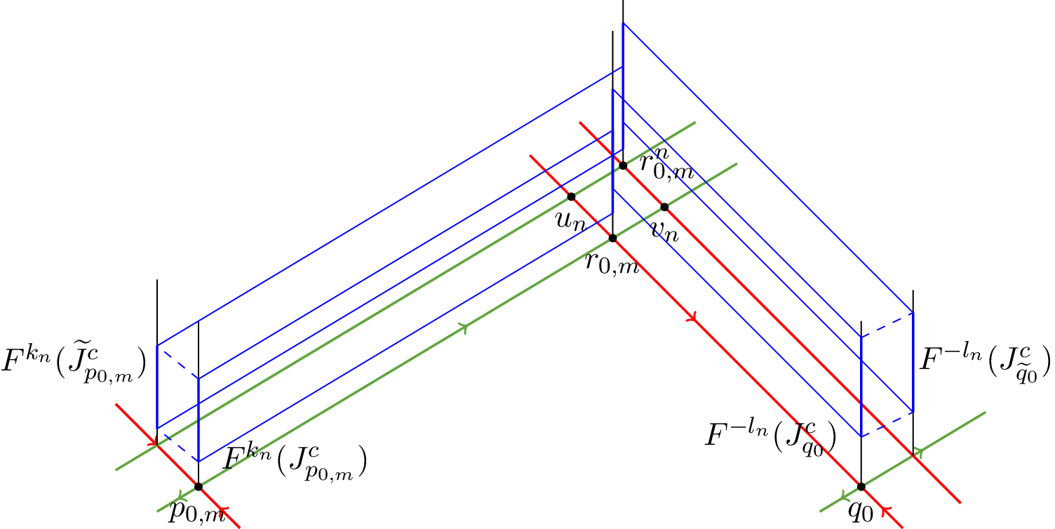
 -leaves or
$cs$
 -leaves, see Figure 7.
Central intersections (color online).

Figure 7 Long description
A three-dimensional diagram illustrating central intersections. At the central vertex is point r sub 0,m. Extending from this center are three colored axes. A green line extends to the bottom-left, ending at point p sub 0,m. A red line extends to the bottom-right, ending at point q sub 0. A vertical black line extends upward.
Along the green axis, a blue rectangular prism is labeled F super k sub n (J super c sub p sub 0,m) at its base and F super k sub n (tilde J super c sub p sub 0,m) at its top. Along the red axis, a similar blue rectangular prism is labeled F super minus l sub n (J super c sub q sub 0) at its base and F super minus l sub n (tilde J super c sub q sub 0) at its top.
Near the central intersection r sub 0,m, there are additional labeled points on the intersecting grid lines. Point u sub n is located on a green line slightly above the main axis. Point v sub n is on a red line to the right of the center. Point r super n sub 0,m is located vertically above the central r sub 0,m point where the upper blue frames intersect. Arrows on the red and green lines indicate directional flow toward and away from the central intersection points.
Claim 3.6. There exist two strictly increasing subsequences
$\{k_n\},\ \{l_n\}$
 of
$\mathbb {N}$
 such that

where

Moreover, there exists a constant
$c> 0$
 such that

Proof of Claim 3.6.
Note that

which means that

since
$p_{0,m}$
 and
$q_0$
 are assumed to be fixed points. Equivalently, we have

The conclusion then follows from Proposition 2.9, by taking

The initial intervals are
$(\gamma _{p_{0,m}}^s)^{-1}(J_{p_{0,m}}^c)$
 and
$(\gamma ^s_{q_0})^{-1}(J_{q_0}^c)$
 .
As a result, there exists a constant
$c> 0$
 such that

where

Now, consider the intersection between
$F^{k_n}(\mathcal {F}^u_{\mathrm {loc}}(\widetilde {J}_{p_{0,m}}^c))$
 and
$F^{-l_n}(\mathcal {F}^s_{\mathrm {loc}}(J_{\widetilde {q}_0}^c))$
 . Since
$F_0$
 is an Anosov diffeomorphism on a nilmanifold, for n sufficiently large, their projections on
$M_0$
 ,
$\pi _0(F^{k_n}(\mathcal {F}^u_{\mathrm {loc}}(\widetilde {J}_{p_{0,m}}^c)))$
 , and
$\pi _0(F^{-l_n}(\mathcal {F}^s_{\mathrm {loc}}(J_{\widetilde {q}_0}^c)))$
 , intersect at
$r_{0,m}^n\in M_0$
 , which converges to
$r_{0,m}$
 as
$n \to +\infty $
 . Moreover, we have

For simplicity, we denote the intersections by

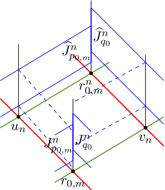
Our aim is to show that
${\widehat {J}_{p_{0,m}}^n}\cap {\widehat {J}_{q_0}^n}\neq \varnothing $
 , see Figure 8.
Dynamics near
$r_{0,m}$
 (color online).

By Lemma 2.1 (the
$C^1$
 property of holonomy maps) and Lemma 2.2 (the estimate of central twists), there exists a constant
$C\geq 1$
 such that

as intervals in
$\mathcal {F}^c(r_{0,m})$
 , where

Again, by the argument of central twist in Lemma 2.2, for n sufficiently large and
$x\in \widehat {J}_q^n$
 , we have

Compared with the length of the intersection which is controlled by

and the preceding perturbation errors, which are
$o(\rho _n)$
 , implied by the strict inequalities among the corresponding Lyapunov exponents, we conclude together with the injectivity of the maps
$\mathrm {Hol}_{u_n}^{r_{0,m}}\circ \mathrm {Hol}_{r_{0,m}^n}^{u_n}$
 and
$\mathrm {Hol}_{v_n}^{r_{0,m}}\circ \mathrm {Hol}_{r_{0,m}^n}^{v_n}$
 that there exists
$n_0\in \mathbb {N}$
 such that
${\widehat {J}_{p_{0,m}}^n}\cap {\widehat {J}_{q_0}^n}\neq \varnothing $
 for any
$n \geq n_0$
 . Since
${\widehat {J}_{p_{0,m}}^n}\subseteq U^*$
 and
${\widehat {J}_{q_0}^n} \subseteq V^*$
 , we have
$U^*\cap V^*\neq \varnothing $
 .
This ends the proof of Theorem 3.1.
Corollary 3.7. If
$F\in \mathrm {PHI}^1(M)$
 is boundary interconnected, then there is an open neighborhood
$\mathcal {U}\subseteq \mathrm {PHI}^1(M)$
 of F such that every
$G\in \mathcal {U}\cap \mathrm {PHI}^2(M)$
 is topologically transitive.
Proof. Notice that the boundary interconnection property is
$C^1$
 -open in
$\mathrm {PHI}^1(M)$
 . The conclusion then follows directly from Theorem 3.1.
4 Robust transitivity implies boundary interconnection
In this section, we complete the proof of Theorem A by showing that robust transitivity implies boundary interconnection.
Theorem 4.1. If
$F\in \mathrm {PHI}^k(M)\ (k \geq 2)$
 is
$C^k$
 -robustly transitive, then F is boundary interconnected.
As a preparation of the proof, we need the following method to construct an attractor by perturbation.
Lemma 4.2. Let
$F\in \mathrm {PHI}^k(M)\ (k \geq 2)$
 . If
$\unicode{x3bb} ^c(p) \leq 0$
 for every
$p\in \mathrm {Per}(F_0)$
 , then for any neighborhood
$\mathcal {U}\subseteq \mathrm {PHI}^k(M)$
 of F, there exists
$G\in \mathcal {U}$
 such that
$M_0$
 is an attractor of G.
Proof. By Corollary 2.7, we have
$\unicode{x3bb} ^c(x) \leq 0$
 whenever
$\unicode{x3bb} ^c(x)$
 exists. To show that
$M_0$
 is an attractor of G, it suffices (see [Reference CaoCao03, Lemma 2]) to check that there exists a constant
$\varepsilon> 0$
 such that

has full measure with respect to any ergodic measure of
$G_0$
 .
Let
$X(s) := s(s - 1)$
 be a
$C^\infty $
 vector field on
$[0,1]$
 and
$\Phi _t(s)$
 be the
$C^\infty $
 flow generated by X. Then, by abuse of notation, we define

It follows that
$\Phi _t$
 converges to identity as
$t\to 0^+$
 , in any
$C^k$
 topology.
Now, consider
$G := \Phi _t\circ F$
 . Since G acts in the same way as F on
$M_0$
 and
$M_1$
 , we have
$G\in \mathrm {Diff}_\partial ^k(M)$
 and, hence, when
$t> 0$
 is sufficiently small,
$G\in \mathrm {PHI}^k(M)$
 .
Note that the partially hyperbolic splitting of G restricted to
$M_0$
 has the same stable and unstable subbundles as F. We denote it by

Define
$\alpha _t := \Phi ^{\prime }_t(0){=\partial _s\Phi _t(0)} \in (0, 1)$
 and
$\beta (z) := f^{\prime }_z(0)=\partial _s f_z(0)> 0$
 , where we denote
$F(z,s)=(F_s(z),f_z(s))$
 . Here,
$\alpha _t=e^{-t}$
 , which can be solved by
$({d}/{dt})\alpha _t=-\alpha _t$
 and
$\alpha _0=1$
 , and hence,
$\alpha _t \in (0, 1)$
 when
$t>0$
 . Then, we have

Let
$v^c = (*, 1)^T$
 and
$v^c_G = (*, 1)^T$
 be vectors of
$E^c(z, 0)$
 and
$E^c_G(z, 0)$
 , respectively. Then,

Let
$\|\cdot \|$
 be the original induced norm in
$E^c$
 and
$E^c_G$
 , and define

Since
$E^c$
 and
$E^c_G$
 are both transverse to
$M_0$
 , which is compact, the norms
$\|\cdot \|_F$
 and
$\|\cdot \|_G$
 are both equivalent with
$\|\cdot \|$
 . That is, there exists a constant
$C \geq 1$
 such that

Moreover, by the above discussion, we have

As a result, for any
$x\in M_0$
 ,

and, hence,

By the classical Oseledets theorem, for each ergodic measure
$\mu $
 of
${F_0 {\kern-1pt}={\kern-1pt} G_0: M_0 {\kern-1pt}\to{\kern-1pt} M_0}$
 , there exists a
$\mu $
 -full measure subset
$B_\mu \subseteq M_0$
 such that for any
$x\in B_\mu $
 , the Lyapunov exponents of F and G at x both exist. Consider

then
$\mu (B_0) = 1$
 for any ergodic measure
$\mu $
 .
Fix
$x\in B_0$
 . We have

Let
$n \to +\infty $
 and we have

This completes the proof of Lemma 4.2.
Proof of Theorem 4.1.
Since F is
$C^k$
 -robustly transitive, there exists an open neighborhood
$\mathcal {U}\subseteq \mathrm {PHI}^k(M)$
 of F such that every
$G\in \mathcal {U}$
 is topologically transitive.
We first prove that there exist
$p_0,\ q_0\in \mathrm {Per}(F_0)$
 such that
$\unicode{x3bb} ^c(p_0) < 0 < \unicode{x3bb} ^c(q_0)$
 . A similar conclusion holds for
$F_1$
 . For contradiction, without loss of generality, we assume that

Then, by Lemma 4.2, there exists a
$C^k$
 -perturbation
$G\in \mathcal {U}$
 such that
$M_0$
 is an attractor of G, which contradicts the topological transitivity of G.
Now, take
$p_0,q_0\in M_0$
 and
$p_1,q_1\in M_1$
 such that

It remains to show that
$W^s(p_0)\cap W^u(p_1)\neq \varnothing $
 and, similarly,
${W^u(q_0)}\cap W^s(q_1)\neq \varnothing $
 .
First, notice that

Since F is topologically transitive, there exists
$x\in M$
 such that

In particular, there exists
$i_0\in \mathbb {Z}$
 such that
$F^{i_0}(x)\in \mathcal {F}^s_{\varepsilon _0}(\mathcal {F}^{cu}_{\mathrm {loc}}(p_1))$
 for some
$\varepsilon _0> 0$
 . Assume that
$F^{i_0}(x)\in \mathcal {F}^s_{\varepsilon _0}(z_1)$
 , where
$z_1\in \mathcal {F}^{cu}_{\mathrm {loc}}(p_1)$
 .
By the density of
$\{F^i(x): i\geq i_0\}$
 , for any
$\varepsilon> 0$
 , there exists
$N\in \mathbb {N}$
 such that
$F^{i_0 + N}(x)\in \mathcal {F}^u_\varepsilon (\mathcal {F}^{cs}_\varepsilon (p_0))$
 . Moreover, for fixed
$\varepsilon> 0$
 , N can be arbitrarily large. By taking
$\varepsilon> 0$
 small, we may assume that

Now, take N large so that
$F^N(z_1)\in \mathcal {F}^s_\varepsilon (F^{i_0 + N}(x))$
 . It follows that
$F^N(z_1)\in \mathcal {F}^u_{\varepsilon _0}(z_0)$
 for some
$z_0\in \mathcal {F}^{cs}_{\mathrm {loc}}(p_0)$
 . Since
$W^u(p_1)$
 is F-invariant and u-saturated, we have
$z_0\in W^s(p_0)\cap W^u(p_1)$
 .
This completes the proof of Theorem 4.1.
5 Intermingled basins
In this section, we prove Theorem B. Recall that for
$F\in \mathrm {PHI}_-^k(M)\ (k \geq 2)$
 , there are boundary SRB measures
$\mu _0$
 on
$M_0$
 and
$\mu _1$
 on
$M_1$
 . For
$i = 0,1$
 , since
$\mu _i$
 is the unique SRB measure of
$F_i: M_i \to M_i$
 , we have the following results:
-
• $\mathrm {supp}(\mu _i) = M_i$
; -
• $B(\mu _i)\cap M_i$
has full Lebesgue measure in
$M_i$
; -
• for any u-segment $\gamma ^u\subseteq M_i$
,
$\gamma ^u\cap B(\mu _i)$
has full Lebesgue measure in
$\gamma ^u$
; -
• there exists $L_i\subseteq M_i$
with positive Lebesgue measure such that
$\unicode{x3bb} ^c(x) < 0\ \text {for all } x\in L_i$
, and consequently,
$|W^s(x)\cap \mathcal {F}^c(x)|> 0\ \text {for all } x\in L_i$
; -
• there exists $K_i\subseteq L_i$
with positive Lebesgue measure such that $$ \begin{align*} \inf_{x\in K_i}|W^s(x)\cap \mathcal{F}^c(x)|> 0. \end{align*} $$


Theorem 5.1. If
$F\in \mathrm {PHI}_-^2(M)$
 is topologically transitive, then F admits intermingled basins.
Proof of Theorem 5.1.
We first prove the following claim.
Claim 5.2. For any
$cu$
 -box
$\mathcal {B}$
 ,
$\mathcal {B}\cap B(\mu _0)$
 has positive Lebesgue measure in
$\mathcal {B}$
 , and further, for any
$cu$
 -box
$\mathcal {B}'$
 that is
$C^1$
 -close to
$\mathcal {B}$
 ,

Proof of Claim 5.2.
Consider the open set
$U = \mathcal {F}^s_\varepsilon (\mathcal {B})$
 . Since F is topologically transitive, given any non-empty open set V,
$F^N(U)\cap V\neq \varnothing $
 for infinitely many
$N\in \mathbb {N}$
 . It follows that
$\bigcup _{n\in \mathbb {N}}F^n(\mathcal {B})$
 is dense in M. In particular, there exists
$N\in \mathbb {N}$
 and a
$cu$
 -box
${\mathcal {P} \subseteq F^N(\mathcal {B})}$
 sufficiently close to
$M_0$
 such that
$\pi _0(\mathcal {P})\cap K_0$
 has positive Lebesgue measure in
$\pi _0(\mathcal {P})$
 and
$x\in W^s(\pi _0(x))$
 for any
$x\in \mathcal {P}$
 with
$\pi _0(x)\in K_0$
 . However,
$\pi _0(\mathcal {P})\cap B(\mu _0)$
 has full Lebesgue measure in
$\pi _0(\mathcal {P})$
 . It follows that
$\mathcal {P}\cap B(\mu _0)$
 has positive Lebesgue measure in
$\mathcal {P}$
 and, hence,
$\mathcal {B}\cap B(\mu _0)$
 also has positive Lebesgue measure in
$\mathcal {B}$
 . Moreover,
$B(\mu _0)$
 is s-saturated, hence, for any
$cu$
 -box
$\mathcal {B}'$
 that is
$C^1$
 close to
$\mathcal {B}$
 ,
$\mathrm {Leb}(\mathcal {B}'\cap B(\mu _0))$
 has a uniform lower bound away from zero, given as above.
A similar result holds for
$B(\mu _1)$
 . Therefore, we conclude that for any non-empty open subset
$U\subseteq M$
 ,
$U\cap B(\mu _0)$
 and
$U\cap B(\mu _1)$
 both have positive Lebesgue measure.
To show that
$B(\mu _0)\cup B(\mu _1)$
 has full Lebesgue measure, assume for contradiction that the complement
$\mathcal {C}$
 has positive Lebesgue measure. Take a density point
$x^*\in M$
 of
$\mathcal {C}$
 . Since the basins are s-saturated, we have

By the above argument, there exists
$N_k \to +\infty $
 and a
$cu$
 -box
$\mathcal {P}_k \subseteq F^{N_k}(\mathcal {F}_{\varepsilon _0}^{cu}(x^*))$
 near
$M_0$
 , with the same size, such that
$\mathcal {P}_k\cap B(\mu _0)$
 consists of central leaves. Moreover, we have that
$F^{-N_k}(\mathcal {P}_k)\subseteq \mathcal {F}^c_{\varepsilon _0}(\mathcal {F}^u_{\varepsilon _k}(x^*))$
 , where
${\varepsilon _k \to 0^+}$
 . Define

Since for each
$k\in \mathbb {N}$
 ,
$\det (DF^{N_k}|_{E^{cu}})$
 is nearly constant on
$\mathcal {F}^{cu}_{\varepsilon _0}(x^*)$
 when
$\varepsilon _0$
 is small, we conclude that

and consequently,

Noting that
$\mathcal {P}_k\cap B(\mu _0)$
 consists of central leaves, we also have

By taking a subsequence, we may assume that
$\mathcal {P}_k$
 converges to a
$cu$
 -box
$\mathcal {P}$
 . This contradicts the fact that a
$cu$
 -box near
$\mathcal {P}$
 intersects
$B(\mu _0)$
 on a subset whose Lebesgue measure has a lower bound away from zero, see Claim 5.2.
Theorem 5.3. If
$F\in \mathrm {PHI}_-^k(M)\ (k \geq 2)$
 admits
$C^k$
 -robustly intermingled basins, then F is boundary interconnected.
Proof of Theorem 5.3.
Since F admits
$C^k$
 -robustly intermingled basins, there exists an open neighborhood
$\mathcal {U}\subseteq \mathrm {PHI}_-^k(M)$
 of F such that every
$G\in \mathcal {U}$
 admits intermingled basins.
We first show that there exist
$q_0\in \mathrm {Per}(F_0)$
 and
$p_1\in \mathrm {Per}(F_1)$
 admitting positive central Lyapunov exponents.
Assume for contradiction that
$\unicode{x3bb} ^c(p) \leq 0$
 for all
$p\in \mathrm {Per}(F_0)$
 . By Lemma 4.2, there exists
$G\in \mathcal {U}$
 such that
$M_0$
 is an attractor of G. Moreover, G acts in the same way as F on
$M_0$
 and
$M_1$
 , hence, the boundary SRB measures of G are also
$\mu _0$
 and
$\mu _1$
 . In this case,
$B_G(\mu _1)$
 cannot be dense near
$M_0$
 , which contradicts the fact that G admits intermingled basins.
Now, we have
$q_0\in \mathrm {Per}(F_0)$
 and
$p_1\in \mathrm {Per}(F_1)$
 with positive central Lyapunov exponents. Fix
$p_0\in \mathrm {Per}(F_0)$
 and
$q_1\in \mathrm {Per}(F_1)$
 with negative central Lyapunov exponents. Since F admits intermingled basins,
$B(\mu _0)\cap \mathcal {F}^{cu}_{\mathrm {loc}}(p_1)$
 has positive Lebesgue measure in
$\mathcal {F}^{cu}_{\mathrm {loc}}(p_1)$
 . By forward iteration, we know that there exists a
$cu$
 -box
$\mathcal {P}\subseteq W^u(p_1)$
 near
$p_0$
 , since we have
$\mathrm {supp}(\mu _0) = M_0$
 . Therefore,
$\mathcal {P}\pitchfork \mathcal {F}^{cs}_{\mathrm {loc}}(p_0)\neq \varnothing $
 , and hence,
$W^u(p_1)\pitchfork W^s(p_0)\neq \varnothing $
 . A similar argument shows that
$W^s(q_1)\pitchfork W^u(q_0)\neq \varnothing $
 . Hence, F is boundary interconnected.


Acknowledgments
The third author is grateful to Sichuan University for the hospitality during his visits when part of the work was done. The authors are grateful to anonymous referees for comments and suggestions which are helpful to improve the presentation of this paper.
Funding
Y.S. was partially supported by the NSFC (12526207 and 12571203); M.X. was partially supported by the NSFC (12501238) and the Fundamental Research Funds for the Central Universities (DUT24RC(3)112).