1. Introduction
Consider a continuous time compound renewal process representing aggregate claims of an insurance portfolio and let
 $$Z_{t} \;{\equals}\;\mathop{\sum}\limits_{i\;{\equals}\;1}^{N_{t} } {\rm e}^{{{\minus}\delta T_{i} }} X_{i}, } \quad t\geq 0$$
be the aggregate discounted value at time 0 of all claims recorded over [0, t], where δ≥0 is the force of interest and
 $T_{n} \;{\equals}\;\mathop{\sum}\nolimits_{i{\equals}1}^n W _{i} $
is the occurrence time of the nth claim. The X
i
’s are i.i.d. random variables with common distribution function F
X
(such that F
X
(0)=0) and density f
X
. We denote its moment generating function by
 $M_{X} (s)\;{\equals}\;{\int}_0^\infty {{\rm e}^{{sx}} f_{X} (x)\,dx} $
. The counting process {N
t
; t≥0} is a renewal process representing the number of claims up to time t and is defined as N
t
=max{n∈ℕ+:W
1+W
2+…+W
n
≤t}, where inter-claim times
 $W_{i}^{\prime} s$
are assumed i.i.d. with common distribution function F
W
(and corresponding density function f
W
). Define
 $$V_{n} (t)\;{\equals}\;{\Bbb E}[Z_{t}^{n} ],\quad t\geq 0,\quad n\in{ℕ}^{{\plus}} $$
to be the nth moment of Z t . Note that V n (0)=0 and V 0(t)=1.
Analysis on the moments and distributions of the discounted aggregate claims in the compound Poisson process can be found in Taylor (Reference Taylor1979), Delbaen & Haezendonck (Reference Delbaen and Haezendonck1987) and Willmot (Reference Willmot1989). Léveillé & Garrido (Reference Léveillé and Garrido2001 a) give explicit expressions for the first two moments of the discounted aggregate claims in the compound renewal risk process by using renewal theory arguments. Further Léveillé & Garrido (Reference Léveillé and Garrido2001 b) give a recursive formula for the moments of a compound renewal present value process. Jang (Reference Jang2004) obtains the Laplace transform of the distribution of the discounted aggregate claims using a shot noise process. Kim & Kim (Reference Kim and Kim2007) give the first two moments of the discounted aggregate claims when the rates of claim arrivals and the claim sizes change according to the states of an underlying Markov process. Ren (Reference Ren2008) obtains some matrix expressions for the Laplace transform and the first two moments of the aggregate discounted claims, when inter-claim times follow a Markovian arrival process (MAP). Léveillé et al. (Reference Léveillé, Garrido and Wang2010) study the moment generating functions of the discounted aggregate claims process in finite time and infinite time. Covariance and joint moments of Z t and Z t+s are discussed in Léveillé & Adékambi (Reference Léveillé and Adékambi2011, Reference Léveillé and Adékambi2012). Wang et al. (Reference Wang, Garrido and Léveillé2016) give more explicit results on this topic and use them to calculate risk measures such as Value-at-Risk and Conditional Tail Expectation.
Attention has also been drawn to the introduction of the dependency within the model. Albrecher & Boxma (Reference Albrecher and Boxma2004) propose dependence between X n and W n+1, i.e., claim size has an impact on the next inter-arrival time. This structure is also investigated in Cheung (Reference Cheung2012). Conversely, Boudreault et al. (Reference Boudreault, Cossette, Landriault and Marceau2006) assume inter-arrival time has effects on the next claim amount. Copula is introduced in Albrecher & Teugels (Reference Albrecher and Teugels2006), and then discussed in Boudreault et al. (Reference Boudreault, Cossette, Landriault and Marceau2006) and Cossette et al. (Reference Cossette, Marceau and Marri2008, Reference Cossette, Marceau and Marri2010).
From literature, it shows that the distribution of Z t for t<∞ is hard to obtain even under independence assumption, let alone under dependent structure. Therefore, the study on the moments of Z t , at least, provides some information for its distribution. Further, if an explicit formula on moments is provided, various moments matching methods can be applied for density approximation purpose.
Barges et al. (Reference Barges, Cossette, Loisel and Marceau2011) investigate the moments of Z t under a compound Poisson process via dependence being measured by the classical Farlie–Gumbel–Morgenstern (FGM) copula which is a special case of the copula defined in the next section and studied in our paper. The results in Barges et al. (Reference Barges, Cossette, Loisel and Marceau2011) are much more complicated and involve multiple summations and significant choice problems for index. Woo & Cheung (Reference Woo and Cheung2013) proposes a dependent risk model in which the conditional pdf of X given W=t can be expressed as a mixture of densities and then the generalised FGM copula is a special case of their model. However, their method requires a large amount of work in identification and calculation of the coefficients, even just under the simplest case, i.e., the classical FGM. Thus, the motivation of this paper is to provide explicit formulas for moments and joint moments of Z t for the generalised FGM copula, with the help of some interesting properties of the Beta transform.
In this paper, section 2 specifies the copula we are going to use, which is the generalisation of Barges et al. (Reference Barges, Cossette, Loisel and Marceau2011). Section 3 revisits a distributional transform, the Beta transform, which is actually a generalisation of the Proportional Hazard (PH) transform in Wang (Reference Wang1995). Later, examples and stochastic ordering properties are presented. Section 4 gives the integral equation for moments and joint moments under this framework. Section 5 gives a few specific results, theoretically and numerically, when the arrival process is a Poisson process, which are more computationed friendly. Section 6 discusses the moments of this discounted aggregated sum when the inter-arrival times follow an Erlang(2) distribution. Section 7 gives some concluding remarks.
2. Dependence Between Inter-Claim Times and Claim Sizes
In the renewal risk model, inter-claim times and claim sizes are assumed to be independent. There exist real-world situations for which such an assumption is inappropriate. Recently, risk models with dependence between inter-claim times and claim sizes have been studied extensively by researchers.
Albrecher & Boxma (Reference Albrecher and Boxma2004) propose an extension to the classical risk model with dependence between inter-claim times and claim sizes in which the distribution of the time between two successive claims depends on the previous claim size and study the Gerber–Shiu function for this dependent risk model. Such a dependent risk model can be transformed to a semi-Markovian risk model which was first introduced in Janssen & Reinhard (Reference Janssen and Reinhard1985) and further studied by Albrecher & Boxma (Reference Albrecher and Boxma2005). This semi-Markovian risk model is a special case of a MAP risk model, see Badescu et al. (Reference Badescu, Breuer, Drekic, Latouche and Stanford2005). The moments of the aggregate discounted claims in a MAP risk model have been studied in Ren (Reference Ren2008).
Boudreault et al. (Reference Boudreault, Cossette, Landriault and Marceau2006) propose an extension to the classical risk model in which a reverse dependent structure was introduced, the distribution of the next claim amount depends on the time elapsed since the last claim, i.e., the conditional distribution of X i given W i =t is given by
 $$f_{{X_{i} ,\mid\,W_{i} \;{\equals}\;t}} (x)\;{\equals}\;{\rm e}^{{{\minus}\beta t}} f_{1} (x){\plus}\left( {1{\minus}{\rm e}^{{{\minus}\beta t}} } \right)f_{2} (x),\quad i\;{\equals}\;1,\,2,\,\ldots\,,\beta \,\gt\,0$$
where f 1 and f 2 are two density functions.
Albrecher & Teugels (Reference Albrecher and Teugels2006) use copulas to define the joint distribution of the inter-claim times and claim sizes. Rodriguez-Lallena & Ãbeda-Flores (Reference Rodriguez-Lallena and Ãbeda-Flores2004) propose the following bivariate copula:
 $$C(u,\,v)\;{\equals}\;uv{\plus}\theta h(u)g(v),\quad u,\,v\,\in\,[0,1]$$
where h and g are non-zero real functions with support [0, 1] satisfying certain conditions and θ is constant. Cossette et al. (Reference Cossette, Marceau and Marri2008) studies the Gerber–Shiu function in the classical risk model with dependence introduced by the copula defined above with a special choice of h and g as follows:
 $$\eqalignno{ & h(u)\;{\equals}\;u^{a} (1{\minus}u)^{b} \cr & g(v)\;{\equals}\;v^{c} (1{\minus}v)^{d} $$
where a, b, c, d≥1, and θ takes values from an interval depending on the values of a, b, c, d. This generalised FGM copula with the above choice of h(u) and g(v) has four parameters with more flexibility in modelling of dependence. In particular, if a=b=c=d=1, then
 $$C(u,\,v)\;{\equals}\;uv{\plus}\theta u(1{\minus}u)v(1{\minus}v),\quad u,\,v\,\in\,[0,\,1]$$
with −1≤θ≤1, is the classical FGM copula, which was discussed in details in Barges et al. (Reference Barges, Cossette, Loisel and Marceau2011).
For h and g defined above, the joint distribution function of (X, W) is
 $$\eqalignno{ F_{{X,W}} (x,\,t)\;{\equals}\; & C\left( {F_{X} (x),\,F_{W} (t)} \right) \cr \;{\equals}\; & F_{X} (x)F_{W} (t){\plus}\theta \left( {F_{X} (x)} \right)^{a} \left[ {1{\minus}F_{X} (x)} \right]^{b} \left( {F_{W} (t)} \right)^{c} \left( {1{\minus}F_{W} (t)} \right)^{d} $$
the joint density function of (X, W) is
 $$f_{{X,W}} (x,\,t)\;{\equals}\;f_{X} (x)f_{W} (t){\plus}\theta h'\left( {F_{X} (x)} \right)g'(F_{W} (t))f_{X} (x)f_{W} (t)$$
and the conditional density of X given that W=t is
 $$f_{{X\,\mid\,W\;{\equals}\;t}} (x)\;{\equals}\;f_{X} (x){\plus}\theta h'\left( {F_{X} (x))f_{X} (x)g'(F_{W} (t)} \right)$$
The covariance of X and W is given by
 $$\eqalignno{ {\rm Cov}(X,\,W) & \;{\equals}\;\mathop{\int}\limits_0^1 {\mathop{\int}\limits_0^1 {\left[ {C(u,\,v){\minus}uv} \right]dF_{X}^{{{\minus}1}} (u)dF_{W}^{{{\minus}1}} (v)} } \cr & \;{\equals}\;\theta \mathop{\int}\limits_0^1 {h(u)dF_{X}^{{{\minus}1}} (u)} \mathop{\int}\limits_0^1 {g(v)dF_{W}^{{{\minus}1}} (v)} $$
This shows that when θ>0 (<0), X and W are positively (negatively) correlated, while when θ=0, X and W are independent.
3. Beta Distributional Transform
In this section, we revisit and study some properties of a distributional transform, the Beta transform. This transform was first proposed in Wirch & Hardy (Reference Wirch and Hardy1999) for distortion functions. Our main results can be expressed in terms of the Beta transforms of distributions of claim inter-arrivals and claim severities. Furthermore, upper and lower bounds for the moments of aggregate discounted claims can obtained by the ordering properties of the Beta transform.
Definition 1 Let X be a positive random variable with probability density function f
X
(x) and cumulative distribution function
 $F_{X} (x)\;{\equals}\;1{\minus}\bar{F}_{X} {(x)} \$
. Define X
(α, β) to be a random variable with probability density function
 $$f_{{X_{{(\alpha ,\;\beta )}} }} \left( x \right)\;{\equals}\;{{{\rm \Gamma }(\alpha {\plus}\beta )} \over {{\rm \Gamma }(\alpha ){\rm \Gamma }(\beta )}}\left[ {F_{X} (x)} \right]^{{\alpha {\minus}1}} \left[\; {\bar{F}_{X} (x)} \right]^{{\beta {\minus}1}} f_{X} (x),\quad \alpha \,\gt\,0,\,\beta \,\gt\,0$$
and probability distribution function
 $$F_{{X_{{(\alpha ,\;\beta )}} }} \left( x \right)\;{\equals}\;{{B\left( {F_{X} (x){;}\,\alpha ,\;\beta } \right)} \over {B\left( {\alpha ,\;\beta } \right)}}$$
where Γ(α), B(α, β) and B(z; α, β) are the gamma function, the beta function and the incomplete beta function, respectively.
Remarks
1. Clearly f X(α, β) (x) and F X(α, β)(x) are probability density function and distribution function, respectively. This distributional transform is called the Beta transform.
2. Random variable X can be generalised on ℝ and the distribution function is still the same. However we restrict X to be positive as it would be claim payment in the following sections.
3. X (1,1) follows the same distribution as the original random variable X.
4. Using a property of the incomplete beta function, we have
(3.3) $$ \bar{F}_{{X_{{(\alpha ,\;\beta )}} }} \left( x \right)\;{\equals}\;{{B\left( {\bar{F}_{X} (x){;}\,\,\beta ,\,\alpha } \right)} \over {B\left( {\alpha ,\;\beta } \right)}}{\rm }$$
5. If α=1, then
$$\bar{F}_{{X_{{(1,\;\beta )}} }} (x)\;{\equals}\;\left[ {\bar{F}_{X} (x)} \right]^{\beta } ,\quad \beta \,\gt\,0$$
The Beta transform is the PH transform. See Wang (Reference Wang1995) for the properties of this transform and its applications.
6. If β=1, then


 $$F_{{X_{{(\alpha ,\;1)}} }} (x)\;{\equals}\;\left[ {F_{X} (x)} \right]^{\alpha } ,\quad \alpha \,\gt\,0$$
This is the dual power transform, see Wirch & Hardy (Reference Wirch and Hardy1999).
The following Lemma shows how to connect F X(α, β) with F X .
Lemma 1. The distribution and the survival function of X (α, β) can be expressed in terms of the hypergeometric function as follows:
 $$F_{{X_{{(\alpha,\,\beta )}} }} \,\left( x \right)\;{\equals}\;{1 \over {\alpha B\left( {\alpha ,\;\beta } \right)}}\left[ {F_{X} (x)} \right]^{\alpha } \,{\rm }_{2} F_{1} \left( {1{\minus}\beta ,\,\alpha {;}\,\,\alpha {\plus}1{;}\,\,F_{X} (x)} \right)$$
 $$\hskip-16pt\;{\equals}\;{1 \over {B\left( {\alpha ,\;\beta } \right)}}\mathop{\sum}\limits_{n\;{\equals}\;0}^\infty {{{\left( {1{\minus}\,\beta } \right)_{n} } \over {n\,!\,}}{{\left[ {F_{X} (x)} \right]^{{n{\plus}\alpha }} } \over {n{\plus}\alpha }}} $$
 $$\bar{F}_{{X_{{(\alpha ,\;\beta )}} }} \left( x \right)\hskip5pt\;{\equals}\;{1 \over {\beta B(\alpha ,\;\beta )}}\left[ {\bar{F}_{X} (x)} \right]^{\beta } \,_{2} F_{1} \left( {1{\minus}\alpha ,\;\beta {;}\,\,\beta {\plus}1{;}\,\,\bar{F}_{X} (x)} \right)$$
 $$\hskip-15pt\;{\equals}\;{1 \over {B\left( {\alpha ,\;\beta } \right)}}\mathop{\sum}\limits_{n\;{\equals}\;0}^\infty {{{\left( {1{\minus}\alpha } \right)_{n} } \over {n\,!\,}}{{\left[ {\bar{F}_{X} (x)} \right]^{{n{\plus}\beta }} } \over {n{\plus}\beta }}} $$
where 2 F 1(a 1, a 2; b 1) is a generalised hypergeometric function with definition
 $${\rm }_{p} F_{q} \left( {a_{1} ,\,a_{2} ,\,\,\ldots\,\,,\,a_{p} {;}\,\,b_{1} ,\,b_{2} ,\,\,\ldots\,\,,\,b_{q} {;}\,\,z} \right)\;{\equals}\;\mathop{\sum}\limits_{m\;{\equals}\;0}^\infty {{{\left( {a_{1} } \right)_{m} \left( {a_{2} } \right)_{m} \,\ldots\,\left( {a_{p} } \right)_{m} } \over {\left( {b_{1} } \right)_{m} \left( {b_{2} } \right)_{m} \,\ldots\,\left( {b_{q} } \right)_{m} }}\,{{z^{m} } \over {m\,!\,}}} $$
and (a) m is the Pochhammer symbol. The moments of X (α, β) can be expressed in terms of the moments of X (1, β+n) as follows:
 $${\Bbb E}\left[ {X_{{(\alpha ,\;\beta )}}^{j} } \right]\;{\equals}\;{1 \over {B\left( {\alpha ,\;\beta } \right)}}\mathop{\sum}\limits_{n\;{\equals}\;0}^\infty {{{\left( {1{\minus}\alpha } \right)_{n} } \over {n\,!\,}}\,{{{\Bbb E}\left[ {X_{{(1,\;\beta {\plus}n)}}^{j} } \right]} \over {\beta {\plus}n}}} {\rm \ztbnd }$$
Proof. Applying the definition of the incomplete beta function and expanding (1−x)(β−1) into the MacLaurin series, we have
 $$B\left( {x{;}\,\,\alpha ,\;\beta } \right)\;{\equals}\;{{x^{\alpha } } \over \alpha }\,_{2} F_{1} \left( {1{\minus}\beta ,\,\alpha {;}\,\,\alpha {\plus}1{;}\,\,x} \right)$$
Using equation (3.2) and the equation above, we obtain equation (3.4). Equation (3.5) is obtained by the definition of 2
F
1 function. Applying similar argument to equation (3.3), we obtain equations (3.6) and (3.7). Equation (3.8) is obtained by noting
 ${\Bbb E}\left[ {X_{{(\alpha ,\;\beta )}}^{j} } \right]\;{\equals}\;j\,{\int}_0^\infty {x^{{j{\minus}1}} \,\bar{F}_{{X_{{(\alpha ,\;\beta )}} }} \left( x \right)dx} .$
This completes the proof.□
Remarks
1.
$\bar{F}_{{X_{{(\alpha ,\;\beta )}} }} (x)$
can be expressed as the infinite mixture of
$\bar{F}_{{X_{{(1, \;\beta {\plus}n)}} }} (x),$
the tail of the PH transformed distribution of X (Remark 5 of Definition 1), for n=0, 1, … .2. If β takes a positive integer value, say β=k, then
$$F_{{X_{{(\alpha ,\;\beta )}} }} \left( x \right)\;{\equals}\;{1 \over {B(\alpha ,\;\beta )}}\mathop{\sum}\limits_{n\;{\equals}\;0}^{k{\minus}1} {{{\left( {1{\minus}\beta } \right)_{n} } \over {n\,!\,}}\,{{\left[ {F_{X} (x)} \right]^{{n{\plus}\alpha }} } \over {n{\plus}\alpha }}} $$
as (1−β) n =(1−k) n =0 when n≥k.
3. If α takes a positive integer value, say α=m, then


 $$\bar{F}_{{X_{{(\alpha ,\;\beta )}} }} \left( x \right)\;{\equals}\;{1 \over {B\left( {\alpha ,\;\beta } \right)}}\mathop{\sum}\limits_{n\;{\equals}\;0}^{m{\minus}1} {{{\left( {1{\minus}\alpha } \right)_{n} } \over {n\,!\,}}\,{{\left[ {\bar{F}_{X} (x)} \right]^{{n{\plus}\beta }} } \over {n{\plus}\beta }}} $$
as (1−α) n =(1−m) n =0 when n≥m.
3.1 Some examples
Example 1. If X~U(0, 1), then
 $$f_{{X_{{(\alpha ,\;\beta )}} }} \left( x \right)\;\;{\equals}\;{{{\rm \Gamma }\left( {\alpha {\plus}\beta } \right)} \over {{\rm \Gamma }\left( \alpha \right){\rm \Gamma }\left( \beta \right)}}x^{{\alpha {\minus}1}} \left( {1{\minus}x} \right)^{{\beta {\minus}1}} ,\quad 0\,\lt\,x\,\lt\,1,\,\alpha \,\gt\,0,\,\beta \,\gt\,0$$
i.e., X (α, β) follows the Beta(α, β) distribution.
Example 2. If X~Exp(η), then
 $\bar{F}_{X} (x)\;{\equals}\;{\rm e}^{{{\minus}\eta x}} $
, and it follows from equation (3.7) that
 $$\bar{F}_{{X_{{(\alpha ,\; {\rm }\beta )}} }} \left( x \right)\;{\equals}\;\mathop{\sum}\limits_{k\;{\equals}\;0}^\infty {\xi _{k} {\rm e}^{{{\minus}\eta (\it k{\plus}\beta )x}} } $$
where
 $$\xi _{k} \;\;{\equals}\;{1 \over {B\left( {\alpha ,\;\beta } \right)}}\,{{\left( {1{\minus}\alpha } \right)_{k} } \over {k\,!\,\left( {k{\plus}\beta } \right)}},\quad k\;{\equals}\;0,\,1,\,2,\,\ldots\,$$
This is to say that X (α, β) follows an infinite mixture of exponential distributions with parameter η(k+β), for k=0, 1, 2, …. The moment generating function
 $$M_{{X_{{(\alpha ,\;\beta )}} }} \left( s \right)\;\;{\equals}\;{{{\rm \Gamma }\left( {\alpha {\plus}\beta } \right){\rm \Gamma }\left( {\beta {\minus}{s \over \eta }} \right)} \over {{\rm \Gamma }\left( \beta \right){\rm \Gamma }\left( {\alpha {\plus}\beta {\minus}{s \over \eta }} \right)}},\quad s\,\lt\,\eta \beta $$
The jth moment of X (α, β) is given by
 $$\eqalignno{ {\Bbb E}\left[ {X_{{(\alpha ,\beta )}}^{j} } \right] & \;{\equals}\;{\eta \over {B\left( {\alpha ,\;\beta } \right)}}\mathop{\sum}\limits_{k\;{\equals}\;0}^\infty {{{\left( {1{\minus}\alpha } \right)_{k} } \over {k\,!\,}}\,{{{\rm \Gamma }\left( {1{\plus}j} \right)} \over {\left( {\eta (k{\plus}\beta )} \right)^{{1{\plus}j}} }}} \cr & \;{\equals}\;{1 \over {B\left( {\alpha ,\;\beta } \right)}}\,{{j\,!\,} \over {\beta ^{{j{\plus}1}} \eta ^{j} }}\,_{{j{\plus}2}} F_{{j{\plus}1}} \left( {1{\minus}\alpha ,\;\beta ,\,\beta ,\,\,\ldots\,\,,\,\beta {;}\,\,\beta {\plus}1,\,\beta {\plus}1,\,\,\ldots\,\,,\,\beta {\plus}1{;}\,\,1} \right) $$
Example 3. If X~Gamma(2, λ), with
 $$f_{X} \left( x \right)\;{\equals}\;\lambda ^{2} x\;{\rm e}^{{{\minus}\lambda x}} ,\quad \bar{F}_{X} \left( x \right)\;{\equals}\;\left( {1{\plus}\lambda x} \right){\rm e}^{{{\minus}\lambda x}} $$
then it follows from (3.7) that
 $$\eqalignno{ \bar{F}_{{X_{{(\alpha ,\;{\rm }\beta )}} }} \left( x \right) & \;{\equals}\;{1 \over {B\left( {\alpha ,\;\beta } \right)}}\mathop{\sum}\limits_{k\;{\equals}\;0}^\infty {{{\left( {1{\minus}\alpha } \right)_{k} } \over {k\,!\,\left( {k{\plus}\beta } \right)}}\left( {1{\plus}\lambda x} \right)^{{(k{\plus}\beta )}} {\rm e}^{{{\minus}\lambda (k{\plus}\beta )x}} } \cr & \;{\equals}\;\mathop{\sum}\limits_{k\;{\equals}\;0}^\infty {\xi _{k} \left( {1{\plus}\lambda x} \right)^{{(k{\plus}\beta )}} {\rm e}^{{{\minus}\lambda (k{\plus}\beta )x}} } $$
where ξ k is given in equation (3.10), and
 $$M_{{X_{{(\alpha ,\;\beta )}} }} \left( s \right)\;{\equals}\;{1 \over {B\left( {\alpha ,\;\beta } \right)}}\mathop{\sum}\limits_{k\;{\equals}\;0}^\infty {{{\left( {1{\minus}\alpha } \right)_{k} } \over {k\,!\,}}U\,\left( {2,\,\beta {\plus}k{\plus}2,\,\beta {\plus}k{\minus}{s \over \lambda }} \right)} ,\quad s\,\lt\,\lambda \left( {\beta {\plus}k} \right)$$
where U(α, γ, z) is the confluent hypergeometric function of the second kind with definition
 $$U\left( {\alpha ,\,\gamma \, {\hbox {;}}\,\,z} \right)\;{\equals}\;{1 \over {{\rm \Gamma }\left( \alpha \right)}}{\int}_0^\infty {{\rm e}^{{{\minus}zt}} t^{{\alpha {\minus}1}} \left( {1{\plus}t} \right)^{{\gamma {\minus}\alpha {\minus}1}} } ,\quad \alpha \,\gt\,0,\quad z\,\gt\,0$$
Example 4. If X~Pareto(γ, η), with
 $$f_{X} \left( x \right)\;{\equals}\;{{\gamma \eta ^{\gamma } } \over {\left( {\eta {\plus}x} \right)^{{\gamma {\plus}1}} }},\quad \bar{F}_{X} \left( x \right)\;{\equals}\;\left( {{\eta \over {\eta {\plus}x}}} \right)^{\gamma } ,\quad x\,\gt\,0,\,\gamma \,\gt\,0{\rm },\,\eta \,\gt\,0$$
then it follows from (3.7) that
 $$\eqalignno{ \bar{F}_{{X_{{(\alpha ,\;{\rm }\beta )}} }} \left( x \right) & \;{\equals}\;{1 \over {B\left( {\alpha ,\;\beta } \right)}}\mathop{\sum}\limits_{k\;{\equals}\;0}^\infty {{{\left( {1{\minus}\alpha } \right)_{k} } \over {k\,!\,\left( {k{\plus}\beta } \right)}}\left( {{\eta \over {\eta {\plus}x}}} \right)^{{\gamma (k{\plus}\beta )}} } \cr & \;{\equals}\;\mathop{\sum}\limits_{k\;{\equals}\;0}^\infty {\xi _{k} \left( {{\eta \over {\eta {\plus}x}}} \right)^{{\gamma (k{\plus}\beta )}} } $$
where ξ k is given in equation (3.10). This is to say, X (α, β), follows an infinite mixture of Pareto distributions with parameters γ(k+β) and η for k=0, 1, 2 …. In particular, when α=1, then X (1, β)~Pareto(γβ, η).
Example 5. If X~Geometric(p), with
 $$f_{X} \left( x \right)\;{\equals}\;pq^{x} ,\quad \bar{F}_{{X}} \left( x \right)\;{\equals}\;q^{{x{\plus}1}} ,\quad 0\,\lt\,p\,\lt\,1,\,p{\plus}q\;{\equals}\;1,\,x\;{\equals}\;0,\,1,\,2,\,\,\ldots\,\,$$
then it follows from (3.7) that
 $$\bar{F}_{{X_{{(\alpha ,\;\beta )}} }} \left( x \right)\;{\equals}\;\mathop{\sum}\limits_{k\;{\equals}\;0}^\infty {\xi _{k} q_{k}^{{x{\plus}1}} } $$
where q k =q k+β , for k=0, 1, 2, …. That is to say, that X (α, β) follows an infinite mixture of geometric distributions with parameter p k =1−q k .
3.2 Stochastic ordering
Next we use the above equations to derive conditions for α and β under which X (α, β) and X are ordered under stochastic ordering and the stop loss ordering. We start with the definitions of these two orderings.
Definition 2 Let X and Y be two non-negative random variables. X, is said to be smaller than Y in the stochastic ordering, denoted as
 $X\,{\preccurlyeq}_{{{\rm st}}} \,Y,$
if
 $\bar{F}_{X} \left( x \right)\leq \bar{F}_{Y} \left( x \right),\,\forall x.$
Definition 3 Let X and Y be two non-negative random variables. X, is said to be smaller than Y, in the convex ordering, denoted as
 $X\,{\preccurlyeq}_{{{\rm sl},\;{\equals}\;}} \,Y,$
or
 $X\,{\preccurlyeq}_{{{\rm cx}}} \,Y,$
if
 ${\Bbb E}\left[ X \right]$
=
 ${\Bbb E}\left[ Y \right]$
, and
 ${\Bbb E}$
[max (X−x, 0)]≤
 ${\Bbb E}$
[max (Y−x, 0)], ∀x ∈ ℝ+ or equivalently, if
 ${\Bbb E}\left[ {\upsilon (X)} \right]\leq {\Bbb E}\left[ {\upsilon (Y)} \right]$
for all convex functions
 $\upsilon $
for which the expectations exist.
Theorem 1. We have the following stochastic ordering between X (α, β) and X.
∙ If α≥1, 0<β<1, then
$X\,{\preccurlyeq}_{{{\rm st}}} \,X_{{(\alpha ,\;\beta )}} $
.∙ If 0<α<1, β≥1, then
$X_{{(\alpha ,\;\beta )}} \,{\preccurlyeq}_{{{\rm st}}} \,X$
.∙ If α=1, β=1, then
$X_{{(\alpha ,\;\beta )}} \mathop{\;{\equals}\;}\limits^{d} X$
.


Proof. It follows from Lebedev (1972, Section 9) that
 $${\rm }_{2} F_{1} \left( {\alpha ,\;\beta {;}\,\,\gamma {;}\,\,1} \right)\;{\equals}\;{{{\rm \Gamma }\left( \gamma \right){\rm \Gamma }\left( {\gamma {\minus}\alpha {\minus}\beta } \right)} \over {{\rm \Gamma }\left( {\gamma {\minus}\alpha } \right){\rm \Gamma }\left( {\gamma {\minus}\beta } \right)}},\quad \Re \left( {\gamma {\minus}\alpha {\minus}\beta } \right)\,\gt\,0{\rm }$$
When α≥1, 0<β<1 it follows from equation (3.4) that
 $$\eqalignno{ F_{{X_{{(\alpha ,\;\beta )}} }} \left( x \right) & \;{\equals}\;{{{\rm \Gamma }(\alpha {\plus}\beta )} \over {{\rm \Gamma }(\alpha {\plus}1){\rm \Gamma }(\beta )}}\left( {F_{X} (x)} \right)^{\alpha } \,_{2} F_{1} \left( {1{\minus}\beta ,\,\alpha ,\,\alpha {\plus}1,\,F_{X} (x)} \right) \cr & \leq {{{\rm \Gamma }(\alpha {\plus}\beta )} \over {{\rm \Gamma }(\alpha {\plus}1){\rm \Gamma }(\beta )}}\left( {F_{X} (x)} \right)^{\alpha } \,_{2} F_{1} (1{\minus}\beta ,\,\alpha ,\,\alpha {\plus}1,\,1) \cr & \;{\equals}\;\left( {F_{X} (x)} \right)^{\alpha } \leq F_{X} (x)\quad \quad \quad (\alpha \geq 1) $$
When 0<α<1, β≥1, equation (3.6) gives
 $$\eqalignno{ \bar{F}_{{X_{{(\alpha ,\;\beta )}} }} \left( x \right) & \;{\equals}\;{{{\rm \Gamma }(\alpha {\plus}\beta )} \over {{\rm \Gamma }(\alpha ){\rm \Gamma }(\beta {\plus}1)}}\left( {\bar{F}_{X} (x)} \right)^{\beta } {\rm }_{2} F_{1} \left( {1{\minus}\alpha ,\;\beta ,\,\beta {\plus}1,\,\bar{F}_{X} (x)} \right) \cr & \leq {{{\rm \Gamma }(\alpha {\plus}\beta )} \over {{\rm \Gamma }(\alpha ){\rm \Gamma }(\beta {\plus}1)}}\left( {\bar{F}_{X} (x)} \right)^{\beta } \,_{2} F_{1} (1{\minus}\alpha ,\;\beta ,\,\beta {\plus}1,\,1) \cr & \;{\equals}\;\left( {\bar{F}_{X} (x)} \right)^{\beta } \leq \bar{F}_{X} (x)\quad \quad \quad (\beta \geq 1) $$
In summary, we have
 $$\bar{F}_{{X_{{(\alpha ,\;\beta )}} }} \left( x \right)\,\left\{ {\matrix{ {\geq \bar{F}_{X} (x),\quad {\rm if}\quad \alpha \geq 1,0\,\lt\,\beta \,\lt\,1} \hfill & {{\rm }} \hfill \cr {\;{\equals}\;\bar{F}_{X} (x),\; \hskip5pt{\rm if}\quad \alpha \;{\equals}\;\beta \;{\equals}\;1} \hfill & {{\rm }} \hfill \cr {\leq \bar{F}_{X} (x),\quad {\rm if}\quad 0\,\lt\,\alpha \,\lt\,1,\beta \geq 1} \hfill & {{\rm }} \hfill \cr } } \right.$$
This proves the stochastic ordering stated in Theorem 1.□
Remark. For j∈ℕ, we have the following inequalities for moments by using the results in Theorem 1
 $${\Bbb E}\left[ {X_{{(\alpha ,\;\beta )}}^{j} } \right]\,\left\{ {\matrix{ {\leq {\Bbb E}[X^{j} ],\quad {\rm if}\quad 0\,\lt\,\alpha \,\lt\,1,\beta \geq 1} \hfill \cr {\geq {\Bbb E}[X^{j} ],\quad {\rm if }\quad \alpha \geq 1,0\,\lt\,\beta \,\lt\,1} \hfill \cr {\;{\equals}\;{\Bbb E}[X^{j} ],\quad \hskip-2pt {\rm if}\quad \alpha \;{\equals}\;\beta \;{\equals}\;1} \hfill \cr } } \right.$$
Theorem 2. Given
 ${\Bbb E}\left[ X \right]$
=
 ${\Bbb E}\left[ {X_{_{{(\alpha ,\;\beta )}} } \right]$
we have the following stochastic ordering between X
(α, β) and X.
∙ If 0<α<1, 0<β<1, then
$X\,{\preccurlyeq}_{{{\rm cx}}} \,X_{{(\alpha ,\;\beta )}} $
.∙ If α>1, β>1, then
$X_{{(\alpha ,\;\beta )}} \,{\preccurlyeq}_{{{\rm cx}}} \,X$
.


Proof. Define
 $$\xi \left( x \right)\;{\equals}\;{{{\rm \Gamma }(\alpha {\plus}\beta )} \over {{\rm \Gamma }(\alpha ){\rm \Gamma }(\beta )}}\left[ {F_{X} (x)} \right]^{{\alpha {\minus}1}} \left[ {1{\minus}F_{X} (x)} \right]^{{\beta {\minus}1}} ,\quad \quad 0\,\lt\,x\,\lt\,\infty,\,\alpha \,\gt\,0,\,\beta \,\gt\,0$$
and then
 $f_{{X_{{(\alpha ,\;\beta )}} }} (x)$
is a weighted version of f
X
(x), i.e.
 $$f_{{X_{{(\alpha ,\;\beta )}} }} \left( x \right)\;{\equals}\;\xi \left( x \right)f_{X} \left( x \right)$$
We discuss the plots for ξ(x) under two cases.
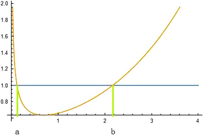
∙ When 0<α<1 and 0<β<1, the plot for ξ(x) is given in Figure 1.
ξ(x) for 0<α<1 and 0<β<1.

It follows from Figure 1 that
 $\xi (a)\;{\equals}\;\xi (b)\;{\equals}\;1$
and
 $$\left\{ {\matrix{ {\xi (x)\,\gt\,1,\quad x\in(0,\,a){\,{\cup}\,} (b,\,\infty)} \hfill \cr {\xi (x)\,\lt\,1,\quad x\in(a,\,b)} \hfill \cr } } \right.$$
That is to say
 $$\left\{ {\matrix{ {f_{{X_{{(\alpha ,\;\beta )}} }} \left( x \right)\,\gt\,f_{X} \left( x \right),\quad x\in(0,\,a){\cup}(b,\,\infty)} \hfill \cr {f_{{X_{{(\alpha ,\;\beta )}} }} \left( x \right)\,\lt\,f_{X} \left( x \right),\quad x\in(a,\,b)} \hfill \cr } } \right.$$
It now follows from theorem 3.A.44 in Shaked & Shanthikumar (Reference Shaked and Shanthikumar2007) that
 $X\,{\preccurlyeq}_{{{\rm cx}}} \,X_{{(\alpha ,\;\beta )}} $
when 0<α<1 and 0<β<1.
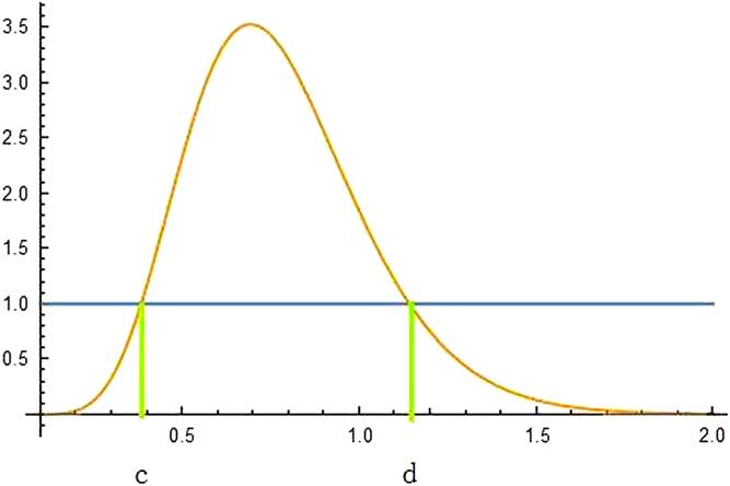
∙ When α>1 and β>1, the plot for ξ(x) is given in Figure 2.
 $\xi (x)$
for α>1 and β>1.

It follows from Figure 2 that ξ(c)=ξ(d)=1 and
 $$\left\{ {\matrix{ {\xi (x)\,\lt\,1,\quad x\in(0,\,c){\cup}(d,\,\infty)} \hfill \cr {\xi (x)\,\gt\,1,\quad x\in(c,\,d)} \hfill \cr } } \right.$$
That is to say
 $$\left\{ {\matrix{ {f_{{X_{{(\alpha ,\;\beta )}} }} (x)\,\lt\,f_{X} (x),\quad x\in(0,\,c){\cup}\left( {c,\,\infty} \right)} \hfill \cr {f_{{X_{{(\alpha ,\;\beta )}} }} (x)\,\gt\,f_{X} (x),\quad x\in(c,\,d)} \hfill \cr } } \right.$$
It now follows from theorem 3.A.44 in Shaked & Shanthikumar (Reference Shaked and Shanthikumar2007) that
 $X_{{(\alpha ,\;\beta )}} \,{\preccurlyeq}_{{{\rm cx}}} \,X$
when α>1 and β>1.
This completes the proof.□
Remarks.
1. Theorems 1 and 2 can be interpreted in the following way:
∙ If α≥1 and 0<β<1, the weighted function ξ(x) increases monotonically. This implies that
$f_{{X_{{(\alpha ,\;\beta )}} }} $
and f
X
cross once and
$f_{{X_{{(\alpha ,\;\beta )}} }} $
is larger than f
X
at the tail, therefore
$\bar{F}_{X} (x)\leq \bar{F}_{{X_{{(\alpha ,\;\beta )}} }} (x)$
for all x, i.e.,
$X\,{\preccurlyeq}_{{{\rm st}}} \,X_{{(\alpha ,\;\beta )}} $
.∙ If 0<α<1 and 0<β<1, ξ(x) decreases first and then increases, as illustrated in Figure 1. This implies that
$f_{{X_{{(\alpha ,\;\beta )}} }} $
and f
X
cross twice and
$\bar{F}_{X} (x)$
and
$\bar{F}_{{X_{{(\alpha ,\;{\rm }\beta )}} }} (x)$
cross once, therefore
$\bar{F}_{X} (x)\leq \bar{F}_{{X_{{(\alpha ,\;{\rm }\beta )}} }} (x)$
for large x, i.e.,
$X\,{\preccurlyeq}_{{{\rm cx}}} \,X_{{(\alpha ,\;\beta )}} $
.∙ Similar reasoning for the other two cases in Theorems 1 and 2.


2. By analysing the monotonicity property of the weight functions between densities, we have
$$\matrix{ {X_{{\left( {\alpha _{1} ,\,\beta } \right)}} {\preccurlyeq}_{{{\rm st}}} \, X_{{\left( {\alpha _{2} ,\,\beta } \right)}} ,} & {0\,\lt\,\alpha _{1} \,\lt\,\alpha _{2} ,\,\beta \,\gt\,0} \cr } $$
and
$$\matrix{ {X_{{\left( {\alpha ,\;\beta _{2} } \right)}} {\preccurlyeq}_{{\rm st}} \, X_{{\left( {\alpha ,\;\beta _{1} } \right)}} ,} & {0\,\lt\,\beta _{1} \,\lt\,\beta _{2} ,\,\alpha \,\gt\,0} \cr } $$
In particular
$$X_{{(\alpha ,\;\beta {\plus}1)}} \,{\preccurlyeq}_{{{\rm st}}} \,X_{{(\alpha ,\;\beta )}} {\preccurlyeq}_{{{\rm st}}} \,X_{{(\alpha {\plus}1,\,\beta )}} $$
3. Further, if
${\Bbb E}\left[ {X_{{(\alpha {\plus}1,\,\beta {\plus}1)}} } \right]\;{\equals}\;{\Bbb E}\left[ {X_{{(\alpha ,\;\beta )}} } \right]$
, then


 $$X_{{(\alpha {\plus}1,\,\beta {\plus}1)}} {\preccurlyeq}_{{{\rm cx}}}\, X_{{(\alpha ,\;\beta )}} $$
This can be obtained by analysing the monotonicity property of ζ(x) where


Finally, when α≥1 and 0<β≤1, the expectation of Beta transform of survival function defines a coherent risk measure, i.e., the mean of the risk adjusted loss of X (α, β). Details could be found in Wirch & Hardy (Reference Wirch and Hardy1999). Related definitions and theorems can be found in Denuit et al. (Reference Denuit, Dhaene, Goovaerts and Kaas2005, section 2) and Tse (Reference Tse2009, section 4).
4. Integral Equations for Moments and Joint Moments
In this section, we aim to provide general formulas for the moments and joint moments of Z t when the joint distribution of (X, W) is defined via the copula defined in section 2. To our knowledge, only few special cases have been done in the literature up to now. When a=b=c=d=1, recursive formulas for moments under Poisson arrival process are discussed in Barges et al. (Reference Barges, Cossette, Loisel and Marceau2011, equation (19)). Later, Woo & Cheung (Reference Woo and Cheung2013, example 3.2) propose a systematic way for this type of dependence structure and give numerical results under a=b=c=d=1 and a=b=c=d=2 cases. However, their method requires a large amount of calculations for coefficients and is therefore not computation friendly.
Define
 $M_{{Z_{t} }} (s)\;{\equals}\;{\Bbb E}\left[ {{\rm e}^{{sZ_{t} }} } \right]$
to be the moment generating function of Z
t
. Using the renewal technique, we have
 $$M_{{Z_{t} }} \left( s \right)\;{\equals}\;{ℙ}\left( {W_{1} \,\gt\,t} \right){\plus}\mathop{\int}\limits_0^t {M_{{X_{1} \;\mid\;W_{1} \;{\equals}\;v}} (se^{{{\minus}\delta v}} )M_{{Z_{{t{\minus}v}} }} (se^{{{\minus}\delta v}} )f_{W} (v)dv} $$
The nth derivative of
 $M_{{Z_{t} }} (s)$
at s is
 $$M_{{Z_{t} }}^{{(n)}} \left( s \right)\;{\equals}\;\mathop \sum\limits_{j\;{\equals}\;0}^n \left( {\matrix{ n \hfill \cr j \hfill \cr } } \right)\mathop \int \limits_0^t {\rm e}^{{{\minus}n\delta v}} M_{{X_{1} \;\mid\;W_{1} \;{\equals}\;v}}^{{(j)}} \left( {se^{{{\minus}\delta v}} } \right)M_{{Z_{{t{\minus}v}} }}^{{(n{\minus}j)}} \left( {se^{{{\minus}\delta v}} } \right)f_{W} (v)dv$$
In order to construct a recursive formula, the term with
 $M_{{Z_{{t{\minus}v}} }}^{{(n)}} \left( {se^{{{\minus}\delta v}} } \right)$
needs to be eliminated and that can be done through the use of convolution. First, we start with rearranging
 $M_{{Z_{t} }}^{{(n)}} (s)$
so that
 $$\hskip-12pt\eqalignno{ M_{{Z_{t} }}^{{(n)}} \left( s \right) \;{\equals}\; \mathop \sum\limits_{j\;{\equals}\;1}^n \left( {\matrix{ n \hfill \cr j \hfill \cr } } \right)\mathop \int \limits_0^t {\rm e}^{{{\minus}n\delta v}} M_{{X_{1} \;\mid\;W_{1} \;{\equals}\;v}}^{{(j)}} \left( {se^{{{\minus}\delta v}} } \right)M_{{Z_{{t{\minus}v}} }}^{{(n{\minus}j)}} \left( {se^{{{\minus}\delta v}} } \right)f_{W} (v)dv \hskip-102pt \cr & \hskip-122pt {\plus}\mathop \int \limits_0^t {\rm e}^{{{\minus}n\delta v}} M_{{Z_{{t{\minus}v}} }}^{{(n)}} \left( {se^{{{\minus}\delta v}} } \right)f_{W} (v)dv $$
Evaluating equation (4.2) at s=0 gives the following result in terms of the moments of Z t :
 $$\eqalignno{ V_{n} \left( t \right)\;{\equals}\; & \mathop \sum\limits_{j\;{\equals}\;1}^n \left( {\matrix{ n \hfill \cr j \hfill \cr } } \right)\mathop \int \limits_0^t {\rm e}^{{{\minus}n\delta v}} {\Bbb E}\left[ {X_{1}^{j} \hskip-2pt\mid\hskip-2ptW_{1} \;{\equals}\;v} \right]V_{{n{\minus}j}} \left( {t{\minus}v} \right)f_{W} \left( v \right)dv \cr & \quad {\plus}\mathop \int \limits_0^t {\rm e}^{{{\minus}n\delta v}} V_{n} \left( {t{\minus}v} \right)f_{W} \left( v \right)dv $$
Under the dependence assumption in equation (2.3):
 $$\eqalignno{ {\Bbb E}\left[ {X_{1}^{j} \hskip-2pt \mid\hskip-2pt W_{1} \;{\equals}\;v} \right] & \;{\equals}\;\mathop{\int}\limits_0^\infty {x^{j} f_{{X_{1} \;\mid\;W_{1} \;{\equals}\;v}} (x)dx} \cr & \;{\equals}\;{\Bbb E}\left[ {X^{j} } \right]{\plus}\theta ac\left[ {F_{W} (v)} \right]^{{c{\minus}1}} \left[ {1{\minus}F_{W} (v)} \right]^{d} \mathop{\int}\limits_0^\infty {x^{j} \left[ {F_{X} (x)} \right]^{{a{\minus}1}} \left[ {1{\minus}F_{X} (x)} \right]^{b} f_{X} (x)dx} \cr {\rm } & \quad \quad {\minus}\theta bc\left[ {F_{W} (v)} \right]^{{c{\minus}1}} \left[ {1{\minus}F_{W} (v)} \right]^{d} \mathop{\int}\limits_0^\infty {x^{j} \left[ {F_{X} (x)} \right]^{a} \left[ {1{\minus}F_{X} (x)} \right]^{{b{\minus}1}} f_{X} (x)dx} \cr & \quad \quad {\minus}\theta ad\left[ {F_{W} (v)} \right]^{c} \left[ {1{\minus}F_{W} (v)} \right]^{{d{\minus}1}} \mathop{\int}\limits_0^\infty {x^{j} \left[ {F_{X} (x)} \right]^{{a{\minus}1}} \left[ {1{\minus}F_{X} (x)} \right]^{b} f_{X} (x)dx} \cr & \quad \quad {\plus}\theta bd\left[ {F_{W} (v)} \right]^{c} \left[ {1{\minus}F_{W} (v)} \right]^{{d{\minus}1}} \mathop{\int}\limits_0^\infty {x^{j} \left[ {F_{X} (x)} \right]^{a} \left[ {1{\minus}F_{X} (x)} \right]^{{b{\minus}1}} f_{X} (x)dx} $$
Applying Definition 1 and using notation X (a, b+1) and X (a, b), we have
 $$\eqalignno{ {\Bbb E}\left[ {X_{1}^{j} \hskip-2pt \mid\hskip-2pt W_{1} \;{\equals}\;v} \right] & \;{\equals}\;{\Bbb E}[X^{j} ]{\plus}\theta ac{{{\rm \Gamma }(a){\rm \Gamma }(b{\plus}1)} \over {{\rm \Gamma }(a{\plus}b{\plus}1)}}[F_{W} (v)]^{{c{\minus}1}} [1{\minus}F_{W} (v)]^{d} {\Bbb E}[X_{{(a,b{\plus}1)}}^{j} ] \cr & \quad \quad {\minus}\theta bc[F_{W} (v)]^{{c{\minus}1}} [1{\minus}F_{W} (v)]^{d} \mathop{\int}\limits_0^\infty {x^{j} \left[ {F_{X} (x)} \right]^{a} \left[ {1{\minus}F_{X} (x)} \right]^{{b{\minus}1}} f_{X} (x)dx} \cr & \quad \quad {\minus}\theta ad{{{\rm \Gamma }(a){\rm \Gamma }(b{\plus}1)} \over {{\rm \Gamma }(a{\plus}b{\plus}1)}}\left[ {F_{W} (v)} \right]^{c} \left[ {1{\minus}F_{W} (v)} \right]^{{d{\minus}1}} {\Bbb E}\left[ {X_{{(a,b{\plus}1)}}^{j} } \right] \cr & \quad \quad {\plus}\theta bd\left[ {F_{W} (v)} \right]^{c} \left[ {1{\minus}F_{W} (v)} \right]^{{d{\minus}1}} \mathop{\int}\limits_0^\infty {x^{j} \left[ {F_{X} (x)} \right]^{a} \left[ {1{\minus}F_{X} (x)} \right]^{{b{\minus}1}} f_{X} (x)dx} \cr & \;\quad \quad {\equals}\;{\Bbb E}[X^{j} ]{\plus}\theta c{{{\rm \Gamma }(a{\plus}1){\rm \Gamma }(b{\plus}1)} \over {{\rm \Gamma }(a{\plus}b{\plus}1)}}[F_{W} (v)]^{{c{\minus}1}} [1{\minus}F_{W} (v)]^{d} {\Bbb E}[X_{{(a,b{\plus}1)}}^{j} ] \cr & \quad \quad {\minus}\theta d{{{\rm \Gamma }(a{\plus}1){\rm \Gamma }(b{\plus}1)} \over {{\rm \Gamma }(a{\plus}b{\plus}1)}}[F_{W} (v)]^{c} [1{\minus}F_{W} (v)]^{{d{\minus}1}} {\Bbb E}[X_{{(a,b{\plus}1)}}^{j} ] \cr & \quad \quad {\plus}\theta bc[F_{W} (v)]^{{c{\minus}1}} [1{\minus}F_{W} (v)]^{d} \mathop{\int}\limits_0^\infty {x^{j} [F_{X} (x)]^{{a{\minus}1}} (1{\minus}F_{X} (x))^{b} f_{X} (x)dx} \cr & \quad \quad {\minus}\theta bd[F_{W} (v)]^{c} [1{\minus}F_{W} (v)]^{{d{\minus}1}} \mathop{\int}\limits_0^\infty {x^{j} \left[ {F_{X} (x)} \right]^{{a{\minus}1}} \left( {1{\minus}F_{X} (x)} \right)^{b} f_{X} ({x})dx} \cr & \quad \quad {\minus}\theta bc{{{\rm \Gamma }(a){\rm \Gamma }(b)} \over {{\rm \Gamma }(a{\plus}b)}}\left[ {F_{W} (v)} \right]^{{c{\minus}1}} \left[ {1{\minus}F_{W} (v)} \right]^{d} {\Bbb E}\left[ {X_{{(a,b)}}^{j} } \right] \cr & \quad \quad {\plus}\theta bd{{{\rm \Gamma }(a){\rm \Gamma }(b)} \over {{\rm \Gamma }(a{\plus}b)}}[F_{W} (v)]^{c} \left[ {1{\minus}F_{W} (v)} \right]^{{d{\minus}1}} {\Bbb E}[X_{{(a,b)}}^{j} ] \cr & \;\quad \quad {\equals}\;{\Bbb E}\left[ {X^{j} } \right]{\plus}\theta c{{{\rm \Gamma }(a){\rm \Gamma }(b{\plus}1)} \over {{\rm \Gamma }(a{\plus}b)}}\left[ {F_{W} (v)} \right]^{{c{\minus}1}} \left[ {1{\minus}F_{W} (v)} \right]^{d} \left( {{\Bbb E}\left[ {X_{{(a,b{\plus}1)}}^{j} } \right]{\minus}{\Bbb E}\left[ {X_{{(a,b)}}^{j} } \right]} \right) \cr & \quad \quad {\minus}\theta d{{{\rm \Gamma }(a){\rm \Gamma }(b{\plus}1)} \over {{\rm \Gamma }(a{\plus}b)}}\left[ {F_{W} (v)} \right]^{c} \left[ {1{\minus}F_{W} (v)} \right]^{{d{\minus}1}} \left( {{\Bbb E}\left[ {X_{{(a,b{\plus}1)}}^{j} } \right]{\minus}{\Bbb E}\left[ {X_{{(a,b)}}^{j} } \right]} \right) $$
When a=b=c=d=1, the equation above is much neater than the expression in Barges et al. (Reference Barges, Cossette, Loisel and Marceau2011) and Woo & Cheung (Reference Woo and Cheung2013). Substituting
 ${\Bbb E}[X_{1}^{j} \hskip-2pt\mid\hskip-2pt W_{1} \;{\equals}\;v]$
into equation (4.3), we have the following equation:
 $$\eqalignno{ V_{n} (t)\;{\equals}\; & \mathop \sum\limits_{j\;{\equals}\;1}^n \left( {\matrix{ n \hfill \cr j \hfill \cr } } \right){\Bbb E}\left[ {X^{j} } \right]\mathop{\int}\limits_0^t {{\rm e}^{{{\minus}n\delta v}} V_{{n{\minus}j}} (t{\minus}v)dF_{W} (v)} \cr &\quad {\plus}\theta c{{{\rm \Gamma }(a){\rm \Gamma }(b{\plus}1)} \over {{\rm \Gamma }(a{\plus}b)}}\mathop \sum\limits_{j\;{\equals}\;1}^n \left( {\matrix{ n \hfill \cr j \hfill \cr } } \right)\left( {{\Bbb E}\left[ {X_{{(a,b{\plus}1)}}^{j} } \right]{\minus}{\Bbb E}\left[ {X_{{(a,\;b)}}^{j} } \right]} \right) \cr & \quad {\times}\mathop{\int}\limits_0^t {{\rm e}^{{{\minus}n\delta v}} \left[ {F_{W} (v)} \right]^{{c{\minus}1}} \left[ {1{\minus}F_{W} (v)} \right]^{d} V_{{n{\minus}j}} (t{\minus}v)dF_{W} (v)} \cr & \quad {\minus}\theta d{{{\rm \Gamma }(a){\rm \Gamma }(b{\plus}1)} \over {{\rm \Gamma }(a{\plus}b)}}\mathop{\sum}\limits_{j\;{\equals}\;1}^n {\left( {\matrix{ n \hfill \cr j \hfill \cr } } \right)\left( {{\Bbb E}\left[ {X_{{(a,b{\plus}1)}}^{j} } \right]{\minus}{\Bbb E}[X_{{(a,\;b)}}^{j} ]} \right)} \cr & \quad {\times}\mathop{\int}\limits_0^t {{\rm e}^{{{\minus}n\delta v}} \left[ {F_{W} (v)} \right]^{c} \left[ {1{\minus}F_{W} (v)} \right]^{{d{\minus}1}} V_{{n{\minus}j}} (t{\minus}v)dF_{W} (v)} \cr & \quad {\plus}\mathop{\int}\limits_0^t {{\rm e}^{{{\minus}n\delta v}} V_{n} (t{\minus}v)dF_{W} (v)} $$
After identifying W (c, d), we have the following result:
Theorem 3. For any δ≥0 and n∈ℕ, the nth moment of Z t satisfies
 $$\eqalignno{ V_{n} (t) & \;{\equals}\;\mathop{\sum}\limits_{j\;{\equals}\;0}^n {\left( {\matrix{ n \hfill \cr j \hfill \cr } } \right){\Bbb E}\left[ {X^{j} } \right]} \mathop{\int}\limits_0^t {{\rm e}^{{{\minus}n\delta v}} V_{{n{\minus}j}} (t{\minus}v)dF_{W} (v)} \cr & \quad \quad {\plus}\theta bcB(a,b)B(c,d{\plus}1)\mathop{\sum}\limits_{j\;{\equals}\;1}^n {\left( {\matrix{ n \hfill \cr j \hfill \cr } } \right)\left( {{\Bbb E}\left[ {X_{{(a,\;b{\plus}1)}}^{j} } \right]{\minus}{\Bbb E}\left[ {X_{{(a,\;b)}}^{j} } \right]} \right)} \cr & \quad \quad {\times}\mathop{\int}\limits_0^t {{\rm e}^{{{\minus}n\delta v}} V_{{n{\minus}j}} (t{\minus}v)dF_{{W_{{(c,d{\plus}1)}} }} (v)} \cr & \quad \quad {\minus} \theta bdB(a,b)B(c{\plus}1,d)\mathop{\sum}\limits_{j\;{\equals}\;1}^n {\left( {\matrix{ n \hfill \cr j \hfill \cr } } \right)\left( {{\Bbb E}\left[ {X_{{(a,\;b{\plus}1)}}^{j} } \right]{\minus}{\Bbb E}\left[ {X_{{(a,\;b)}}^{j} } \right]} \right)} \cr & \quad \quad {\times}\mathop{\int}\limits_0^t {{\rm e}^{{{\minus}n\delta v}} V_{{n{\minus}j}} (t{\minus}v)dF_{{W_{{(c{\plus}1,d)}} }} (v)} $$
Remarks.
1. As the expressions for the Beta transform of f W . and for the moments of the Beta transform of f X have been given in previous section, the recursion formula given in equation (4.5) can be evaluated efficiently by using numerical integration method and using the starting value V 0(t)=1.
2. When the distribution of W is specified, equation (4.5) can be further simplified. In sections 5 and 6, we deal with the cases where
$W\,\sim\,Exp(\lambda )$
and
$W\,\sim\,\Gamma(2,\lambda ).$
Explicit expressions for the moments in particular the lower moments can be derived.


Theorem 3 suggests that, because of Beta transform, the computational capacity of V
n
(t) depends on
 $f_{{W_{{(c,d)}} }} $
. In particular, we have seen in equation (3.6) and will see in the following sections, whether c is an integer or not makes a significant difference in calculation of
 $f_{{W_{{(c,d)}} }} $
. With the aid of stochastic ordering properties obtained in section 3.2, lower and upper bounds for V
n
(t) can be derived when c is not an integer. The following lemma is developed for this purpose.
Lemma 2. Let ϕ be a non-negative and non-decreasing function defined on (−∞, ∞) with ϕ(∞) <∞. Let Y
1 and Y
2 be two positive random variables with corresponding density functions
 $f_{{Y_{1} }} $
and
 $f_{{Y_{2} }} $
. If there exists a positive number m, such that
 $f_{{Y_{2} }} (y)\,\lt\,f_{{Y_{1} }} (y),y\,\lt\,m,$
and
 $f_{{Y_{1} }} (y)\,\lt\,f_{{Y_{2} }} (y),y\,\gt\,m,$
i.e.,
 $Y_{1} {\preccurlyeq}_{{st}} Y_{2} ,$
then
 $$\mathop{\int}\limits_0^t {{\rm e}^{{{\minus}rv}} \phi (t{\minus}v)f_{{Y_{1} }} (v)dv} \geq \mathop{\int}\limits_0^t {{\rm e}^{{{\minus}rv}} \phi (t{\minus}v)f_{{Y_{2} }} (v)dv} ,\quad t\geq 0,r\,\gt\,0$$
Proof. Clearly, inequality (4.6) is true for t≤m. For t>m, the following inequality is true:
 $$\mathop{\int}\limits_t^\infty {{\rm e}^{{{\minus}rv}} \phi (t{\minus}v)f_{{Y_{1} }} (v)dv} \leq \mathop{\int}\limits_t^\infty {{\rm e}^{{{\minus}rv}} \phi (t{\minus}v)f_{{Y_{2} }} (v)dv} $$
Consider function
 $\psi (v)\;{\equals}\;{\rm e}^{{{\minus}rv}} \phi (t{\minus}v),\,0\,\lt\,v\,\lt\,\infty.$
As
 $\psi '(v)\;{\equals}\;{\minus}re^{{{\minus}rv}} \phi (t{\minus}v){\minus}{\rm e}^{{{\minus}rv}} \phi '(t{\minus}v)\leq 0,$
then ψ(ν) is a non-increasing function. It follows from theorem 1.A.3(a) in Shaked & Shanthikumar (Reference Shaked and Shanthikumar2007) that
 $\psi (Y_{2} ){\preccurlyeq}_{{{\rm st}}} \;\psi (Y_{1} )$
, therefore
 ${\Bbb E}[\psi (Y_{2} )]\leq {\Bbb E}[\psi (Y_{1} )]$
and this gives
 $$\mathop{\int}\limits_0^\infty {{\rm e}^{{{\minus}rv}} \phi (t{\minus}v)f_{{Y_{2} }} (v)dv} \leq \mathop{\int}\limits_0^\infty {{\rm e}^{{{\minus}rv}} \phi (t{\minus}v)f_{{Y_{1} }} (v)dv} $$
Combining (4.7) and (4.8) shows that inequality (4.6) is also true for t>m and the proof is completed.□
Now we derive upper and lower bounds for V
n
(t) by using Lemma 2. By the second remark on Theorem 2, we have
 $X_{{(a,b{\plus}1)}} {\preccurlyeq}_{{{\rm st}}} \;X_{{(a,b)}} $
, therefore
 ${\Bbb E}[X_{{(a,b{\plus}1)}}^{j} ]{\minus}{\Bbb E}[X_{{(a,b)}}^{j} ]\,\lt\,0$
. If θ< 0(>0), following Lemma 2, V
n
(t) has the following lower (upper) bound:
 $$\eqalignno{ V_{n} (t) & \geq (\leq )\mathop \sum\limits_{j\;{\equals}\;0}^n \left( {\matrix{ n \hfill \cr j \hfill \cr } } \right){\Bbb E}[X^{j} ]\mathop{\int}\limits_0^t {{\rm e}^{{{\minus}n\delta v}} V_{{n{\minus}j}} (t{\minus}v)dF_{W} (v)} \cr & \quad \quad \quad {\plus}\theta bcB(a,b)B(c,d{\plus}1)\mathop{\sum}\limits_{j\;{\equals}\;1}^n {\left( {\matrix{ n \hfill \cr j \hfill \cr } } \right)\left( {{\Bbb E}\left[ {X_{{(a,b{\plus}1)}}^{j} } \right]{\minus}{\Bbb E}\left[ {X_{{(a,b)}}^{j} } \right]} \right)} \cr & \quad \quad \quad {\times}\mathop{\int}\limits_0^t {{\rm e}^{{{\minus}n\delta v}} V_{{n{\minus}j}} (t{\minus}v)dF_{{W_{{\left( {\left[ c \right]{\plus}1,d{\plus}1} \right)}} }} (v)} \cr & \quad \quad \quad {\minus}\theta bdB(a,b)B(c{\plus}1,d)\mathop{\sum}\limits_{j\;{\equals}\;1}^n {\left( {\matrix{ n \hfill \cr j \hfill \cr } } \right)\left( {{\Bbb E}\left[ {X_{{(a,b{\plus}1)}}^{j} } \right]{\minus}{\Bbb E}\left[ {X_{{(a,b)}}^{j} } \right]} \right)} \cr & \quad \quad \quad {\times}\mathop{\int}\limits_0^t {{\rm e}^{{{\minus}n\delta v}} V_{{n{\minus}j}} (t{\minus}v)dF_{{W_{{\left( {\left[ c \right]{\plus}1,d} \right)}} }} (v)} $$
and the upper (lower) bound
 $$\eqalignno{ V_{n} (t) & \leq (\geq )\mathop \sum\limits_{j\;{\equals}\;0}^n \left( {\matrix{ n \hfill \cr j \hfill \cr } } \right){\Bbb E}[X^{j} ]\mathop \int \limits_0^t {\rm e}^{{{\minus}n\delta v}} V_{{n{\minus}j}} (t{\minus}v)dF_{W} (v) \cr & \quad \quad \quad {\plus}\theta bcB(a,b)B(c,d{\plus}1)\mathop \sum\limits_{j\;{\equals}\;1}^n \left( {\matrix{ n \hfill \cr j \hfill \cr } } \right)({\Bbb E}[X_{{(a,b{\plus}1)}}^{j} ]{\minus}{\Bbb E}[X_{{(a,b)}}^{j} ]) \cr & \quad \quad \quad {\times}\mathop \int \limits_0^t {\rm e}^{{{\minus}n\delta v}} V_{{n{\minus}j}} (t{\minus}v)dF_{{W_{{(\left\lfloor c \right\rfloor,d{\plus}1)}} }} (v) \cr & \quad \quad \quad {\minus}\theta bdB(a,b)B(c{\plus}1,d)\mathop \sum\limits_{j\;{\equals}\;1}^n \left( {\matrix{ n \hfill \cr j \hfill \cr } } \right)({\Bbb E}[X_{{(a,b{\plus}1)}}^{j} ]{\minus}{\Bbb E}[X_{{(a,b)}}^{j} ]) \cr & \quad \quad \quad {\times}\mathop \int \limits_0^t {\rm e}^{{{\minus}n\delta v}} V_{{n{\minus}j}} (t{\minus}v)dF_{{W_{{(\left[ c \right]{\plus}2,d)}} }} (v) $$
where [c] is the integer part of c.
Now we study the joint moments of Z t and Z t+h by starting with their joint moment generating function.
 $$\eqalignno{ M_{{Z_{t} ,Z_{{t{\plus}h}} }} (s,r)\;{\equals}\; & {\Bbb E}\left[ {{\rm e}^{{sZ_{t} {\plus}rZ_{{t{\plus}h}} }} } \right]\;{\equals}\;{\Bbb E}\left[ {{\Bbb E}\left[ {{\rm e}^{{(s{\plus}r)\mathop{\sum}\limits_{k\;{\equals}\;1}^{N_{t} } {{\rm \ztbnd }{\rm e}^{{{\minus}\delta T_{k} }} X_{k} } {\plus}r\mathop{\sum}\limits_{k\;{\equals}\;N_{t} {\plus}1}^{N_{{t{\plus}h}} } {{\rm e}^{{{\minus}\delta T_{k} }} X_{k} } }} \hskip-2pt\mid\hskip-2ptW_{1} } \right]} \right] \cr \;{\equals}\; & \mathop{\int}\limits_0^t {{\Bbb E}\left[ {{\rm e}^{{(s{\plus}r)\mathop{\sum}\limits_{k\;{\equals}\;1}^{N_{t} } {{\rm e}^{{{\minus}\delta T_{k} }} X_{k} } {\plus}r\mathop{\sum}\limits_{k\;{\equals}\;N_{t} {\plus}1}^{N_{{t{\plus}h}} } {{\rm \ztbnd }{\rm e}^{{{\minus}\delta T_{k} }} X_{k} } }} \hskip-2pt\mid\hskip-2ptW_{1} } \right]dF_{W} (v)} \cr & \quad {\plus}\mathop{\int}\limits_t^{t{\plus}h} {{\Bbb E}\left[ {{\rm e}^{{r\mathop{\sum}\limits_{k\;{\equals}\;1}^{N_{{t{\plus}h}} } {{\rm e}^{{{\minus}\delta T_{k} }} X_{k} } }} \hskip-2pt\mid\hskip-2ptW_{1} } \right]dF_{W} (v)} {\plus}\mathop{\int}\limits_{t{\plus}h}^\infty {{\Bbb E}\left[ {\left. {{\rm e}^{0} } \right|W_{1} } \right]dF_{W} (v)} \cr \;{\equals}\; & \mathop{\int}\limits_0^t {{\Bbb E}\left[ {{\rm e}^{{(s{\plus}r){\rm e}^{{{\minus}\delta v}} X_{1} }} \hskip-2pt\mid\hskip-2ptW_{1} } \right]{\Bbb E}\left[ {{\rm e}^{{(s{\plus}r){\rm e}^{{{\minus}\delta v}} \mathop{\sum}\limits_{k\;{\equals}\;2}^{N_{t} } {{\rm e}^{{{\minus}\delta \left( {T_{k} {\minus}v} \right)}} X_{k} } {\plus}re^{{{\minus}\delta v}} \mathop{\sum}\limits_{k\;{\equals}\;N_{t} {\plus}1}^{N_{{t{\plus}h}} } {{\rm \ztbnd }{\rm e}^{{{\minus}\delta \left( {T_{k} {\minus}v} \right)}} X_{k} } }} } \right]dF_{W} (v)} \cr & \quad {\plus}\mathop{\int}\limits_t^{t{\plus}h} {{\Bbb E}\left[ {{\rm e}^{{re^{{{\minus}\delta v}} X_{1} }} \hskip-2pt\mid\hskip-2ptW_{1} } \right]{\Bbb E}\left[ {{\rm e}^{{re^{{{\minus}\delta v}} \mathop{\sum}\limits_{k\;{\equals}\;2}^{N_{{t{\plus}h}} } {{\rm \ztbnd }{\rm e}^{{{\minus}\delta \left( {T_{k} {\minus}v} \right)}} X_{k} } }} } \right]dF_{W} (v)} {\plus}\mathop{\int}\limits_{t{\plus}h}^\infty {dF_{W} (v)} \cr \;{\equals}\; & \mathop{\int}\limits_0^t {{\Bbb E}\left[ {{\rm e}^{{(s{\plus}r){\rm e}^{{{\minus}\delta v}} X_{1} }} \hskip-2pt\mid\hskip-2ptW_{1} } \right]M_{{Z_{{t{\minus}v}} ,\; Z_{{t{\minus}v{\plus}h}} }} \left( {se^{{{\minus}\delta v}} ,re^{{{\minus}\delta v}} } \right)dF_{W} (v)} \cr & \quad {\plus}\mathop{\int}\limits_t^{t{\plus}h} {{\Bbb E}\left[ {{\rm e}^{{re^{{{\minus}\delta v}} X_{1} }} \hskip-2pt\mid\hskip-2ptW_{1} } \right]M_{{Z_{{t{\minus}v{\plus}h}} }} \left( {re^{{{\minus}\delta v}} } \right)dF_{W} (v)} {\plus}\mathop{\int}\limits_{t{\plus}h}^\infty {dF_{W} (v)} $$
Similar to
 ${\Bbb E}\left[ {\left. {X^{j} } \right|W_{1} \;{\equals}\;v} \right]$
, we have
 $$\eqalignno{ {\Bbb E}[ {\rm e}^{{(s{\plus}r){\rm e}^{{{\minus}\delta v}} X_{1} }} \hskip-2pt\mid\hskip-2ptW_{1} ]\;{\equals}\; & M_{X} \left( {(s{\plus}r){\rm e}^{{{\minus}\delta v}} } \right) \cr & \quad {\plus}\theta {{\Gamma (a)\Gamma (1{\plus}b)} \over {\Gamma (a{\plus}b)}}\left( {M_{{X_{{(a,b{\plus}1)}} }} \left( {(s{\plus}r){\rm e}^{{{\minus}\delta v}} } \right){\minus}M_{{X_{{(a,\,b)}} }} \left( {(s{\plus}r){\rm e}^{{{\minus}\delta v}} } \right)} \right) \cr & \quad {\times}\left[ {cF_{W} (v)^{{c{\minus}1}} \left( {1{\minus}F_{W} (v)} \right)^{d} {\minus}dF_{W} (v)^{c} \left( {1{\minus}F_{W} (v)} \right)^{{d{\minus}1}} } \right] $$
Same reasoning for
 ${\Bbb E}[{\rm e}^{{re^{{{\minus}\delta v}} X_{1} }} \hskip-2pt\mid\hskip-2ptW_{1} ]$
. A quick check that could be done for equation (4.9) is to let θ=0, i.e. X
k
and W
k
are independent, then it reduces to Léveillé & Adékambi (Reference Léveillé and Adékambi2012, equation (2.5)). Differentiating
 $M_{{Z_{t} ,{\rm }Z_{{t{\plus}h}} }} (s,\,r)$
with respect to s and r, n and m times, respectively, and then letting s=r=0, we have the following result.
Theorem 4. For any δ≥0, and n, m∈ℕ, the expression of joint moments between Z t and Z t+h is given by
 $$\eqalignno{ V_{{n,m}} (t, t{\plus}h) \;{\equals}\; & \mathop \sum\limits_{k\;{\equals}\;0}^n \mathop \sum\limits_{j\;{\equals}\;0}^m \left( {\matrix{ n \hfill \cr k \hfill \cr } } \right)\left( {\matrix{ m \hfill \cr j \hfill \cr } } \right){\Bbb E}\left[ {X^{{k{\plus}j}} } \right]\mathop{\int}\limits_0^t {{\rm e}^{{{\minus}(n{\plus}m)\delta v}} V_{{n{\minus}k, m{\minus}j}} (t{\minus}v,t{\minus}v{\plus}h)dF_{W} (v)} \cr & \quad {\plus}\theta bcB(a,b)B(c,d{\plus}1)\mathop \sum\limits_{k\;{\equals}\;0}^n \mathop \sum\limits_{j\;{\equals}\;0}^m \left( {\matrix{ n \hfill \cr k \hfill \cr } } \right)\left( {\matrix{ m \hfill \cr j \hfill \cr } } \right)\left( {{\Bbb E}\left[ {X_{{(a,b{\plus}1)}}^{{k{\plus}j}} } \right]{\minus}{\Bbb E}\left[ {X_{{(a,b)}}^{{k{\plus}j}} } \right]} \right) \cr & \quad{\times}\mathop{\int}\limits_0^t {{\rm e}^{{{\minus}(n{\plus}m)\delta v}} V_{{n{\minus}k,m{\minus}j}} (t{\minus}v,t{\minus}v{\plus}h)dF_{{W_{{(c,d{\plus}1)}} }} (v)} \cr & \quad{\minus}\theta bdB(a,b)B(c{\plus}1,d)\mathop \sum\limits_{k\;{\equals}\;0}^n \mathop \sum\limits_{j\;{\equals}\;0}^m \left( {\matrix{ n \hfill \cr k \hfill \cr } } \right)\left( {\matrix{ m \hfill \cr j \hfill \cr } } \right)\left( {{\Bbb E}\left[ {X_{{(a,b{\plus}1)}}^{{k{\plus}j}} } \right]{\minus}{\Bbb E}\left[ {X_{{(a,b)}}^{{k{\plus}j}} } \right]} \right) \cr & \quad{\times}\mathop{\int}\limits_0^t {{\rm e}^{{{\minus}(n{\plus}m)\delta v}} V_{{n{\minus}k,m{\minus}j}} (t{\minus}v,t{\minus}v{\plus}h)dF_{{W_{{(c{\plus}1,d)}} }} (v)} $$
Similar to equation (4.5), equation (4.11) can be evaluated recursively by using numerical integration and noting that V 0,0(t, t+h)=1. In particular, if the counting process is a Poisson process, the joint moments can be further simplified and V 1,1(t, t+h) can be found explicitly. Bounds issue of V n,m (t, t+h) can be discussed similarly to V n (t).
5. Explicit Results Under Poisson Process
In this section, we aim to simplify the results in section 4 to obtain moments and joint moments of the aggregate discounted claims if W follows an exponential distribution with parameter λ>0.
5.1 Simplified expressions for moments and joint moments
We use
 ${\cal L}_{r} \left\{ {z(t)} \right\}\;{\equals}\;\mathop{\int}\limits_0^\infty {{\rm e}^{{{\minus}rt}} z(t)dt} $
to denote the Laplace transform of function z(t).
Lemma 3. A recursive formula for the Laplace transform of the nth moment of Z t with respect to t with parameter r is
 $$\eqalignno{ {\cal L}_{r} \left\{ {V_{n} (t)} \right\}\;{\equals}\; & \mathop \sum\limits_{j\;{\equals}\;1}^n \left( {\matrix{ n \hfill \cr j \hfill \cr } } \right){\Bbb E}\left[ {X^{j} } \right]{\lambda \over {r{\plus}n\delta }}{\cal L}_{r} \left\{ {V_{{n{\minus}j}} (t)} \right\} \cr & {\plus}\theta c{{\Gamma (a)\Gamma (1{\plus}b)} \over {\Gamma (a{\plus}b)}}\mathop \sum\limits_{j\;{\equals}\;1}^n \left( {\matrix{ n \hfill \cr j \hfill \cr } } \right)\left( {{\Bbb E}\left[ {X_{{(a,b{\plus}1)}}^{j} } \right]{\minus}{\Bbb E}\left[ {X_{{(a,b)}}^{j} } \right]} \right) \cr & {\times}{{r{\plus}n\delta {\plus}\lambda } \over {(r{\plus}n\delta )}}B\left( {c,1{\plus}d{\plus}{{r{\plus}n\delta } \over \lambda }} \right){\cal L}_{r} \left\{ {V_{{n{\minus}j}} (t)} \right\} \cr & {\minus}\theta d{{\Gamma (a)\Gamma (1{\plus}b)} \over {\Gamma (a{\plus}b)}}\mathop \sum\limits_{j\;{\equals}\;1}^n \left( {\matrix{ n \hfill \cr j \hfill \cr } } \right)({\Bbb E}[X_{{(a,b{\plus}1)}}^{j} ]{\minus}{\Bbb E}[X_{{(a,b)}}^{j} ]) \cr & {\times}{{r{\plus}n\delta {\plus}\lambda } \over {r{\plus}n\delta }}B\left( {1{\plus}c,d{\plus}{{r{\plus}n\delta } \over \lambda }} \right){\cal L}_{r} \left\{ {V_{{n{\minus}j}} (t)} \right\} $$
Proof. The following integral is frequently used in this case
 $$\mathop{\int}\limits_0^\infty {{\rm e}^{{{\minus}rv}} {\rm e}^{{{\minus}(d{\minus}1)\lambda v}} \left( {1{\minus}e^{{{\minus}\lambda v}} } \right)^{c} dv} \;{\equals}\;{1 \over \lambda }\,{{\Gamma (c{\plus}1)\Gamma \left( {{r \over \lambda }{\plus}d{\minus}1} \right)} \over {\Gamma \left( {c{\plus}{r \over \lambda }{\plus}d} \right)}}\;{\equals}\;{1 \over \lambda }B\,\left( {c{\plus}1,\,{r \over \lambda }{\plus}d{\minus}1} \right)$$
which can be done by a change of variable u=e−λν . Then apply the Laplace transform in Theorem 3 and the result follows after direct calculations.□
Inverting the Laplace transform in Lemma 3, we obtain the following result:
Theorem 5. For any δ≥0 and n∈ℕ, a recursive formula for the nth moment of Z t is
 $$\eqalignno{ V_{n} (t)\;{\equals}\; & \mathop{\sum}\limits_{j\;{\equals}\;1}^n {\left( {\matrix{ n \hfill \cr j \hfill \cr } } \right){\Bbb E}\left[ {X^{j} } \right]} \mathop{\int}\limits_0^t {\lambda {\rm e}^{{{\minus}n\delta v}} V_{{n{\minus}j}} (t{\minus}v)dv} \cr & {\plus}\theta c{{\Gamma (a)\Gamma (1{\plus}b)} \over {\Gamma (a{\plus}b)}}\mathop{\sum}\limits_{j\;{\equals}\;1}^n {\left( {\matrix{ n \hfill \cr j \hfill \cr } } \right)\left( {{\Bbb E}\left[ {X_{{(a,b{\plus}1)}}^{j} } \right]{\minus}{\Bbb E}\left[ {X_{{(a,b)}}^{j} } \right]} \right)} \cr & {\times}\mathop{\sum}\limits_{k\;{\equals}\;0}^\infty {{{(1{\minus}c)_{k} } \over {k\,!\,}}} \mathop{\int}\limits_0^t {\lambda {\rm e}^{{{\minus}n\delta v}} {{1{\plus}e^{{{\minus}(1{\plus}d{\plus}k)\lambda v}} (d{\plus}k)} \over {1{\plus}d{\plus}k}}V_{{n{\minus}j}} (t{\minus}v)dv} \cr & {\minus}\theta d{{\Gamma (a)\Gamma (1{\plus}b)} \over {\Gamma (a{\plus}b)}}\mathop{\sum}\limits_{j\;{\equals}\;1}^n {\left( {\matrix{ n \hfill \cr j \hfill \cr } } \right)\left( {{\Bbb E}\left[ {X_{{(a,b{\plus}1)}}^{j} } \right]{\minus}{\Bbb E}\left[ {X_{{(a,b)}}^{j} } \right]} \right)} \cr & {\times}\mathop{\sum}\limits_{k\;{\equals}\;0}^\infty {{{({\minus}c)_{k} } \over {k\,!\,}}} \mathop{\int}\limits_0^t {\lambda {\rm e}^{{{\minus}n\delta v}} {{1{\plus}e^{{{\minus}(d{\plus}k)\lambda v}} ({\minus}1{\plus}d{\plus}k)} \over {d{\plus}k}}V_{{n{\minus}j}} (t{\minus}v)dv} $$
Proof. Inverting Lemma 3 gives
 $$\eqalignno{ V_{n} (t)\;{\equals}\; & \mathop \sum\limits_{j\;{\equals}\;1}^n \left( {\matrix{ n \hfill \cr j \hfill \cr } } \right){\Bbb E}\left[ {X^{j} } \right]\mathop{\int}\limits_0^t {\lambda {\rm e}^{{{\minus}n\delta v}} V_{{n{\minus}j}} (t{\minus}v)dv} \cr & \quad \quad {\plus}\theta c{{{\rm \Gamma }(a){\rm \Gamma }(1{\plus}b)} \over {{\rm \Gamma }(a{\plus}b)}}\mathop{\sum}\limits_{j\;{\equals}\;1}^n {\left( {\matrix{ n \hfill \cr j \hfill \cr } } \right)\left( {{\Bbb E}\left[ {X_{{(a,b{\plus}1)}}^{j} } \right]{\minus}{\Bbb E}\left[ {X_{{(a,b)}}^{j} } \right]} \right)} \cr &\quad \quad {\times}\left[ {\mathop{\int}\limits_0^{t} {\lambda {\rm e}^{{{\minus}n\delta v}} \left( {1{\minus}{\rm e}^{{{\minus}\lambda v}} } \right)^{{c{\minus}1}} {\rm e}^{{{\minus}d\lambda v}} {\rm e}^{{{\minus}\lambda v}} V_{{n{\minus}j}} (t{\minus}v)dv} } \right. \cr &\left. \quad \quad {{\plus}\mathop{\int}\limits_0^t {\lambda ^{2} {\rm e}^{{{\minus}n\delta v}} \left( {\mathop{\int}\limits_0^v {\left( {1{\minus}{\rm e}^{{{\minus}\lambda u}} } \right)^{{c{\minus}1}} {\rm e}^{{{\minus}d\lambda u}} {\rm e}^{{{\minus}\lambda u}} du} } \right)V_{{n{\minus}j}} (t{\minus}v)dv} } \right] \cr &\quad \quad {\minus}\theta d{{{\rm \Gamma }(a){\rm \Gamma }(1{\plus}b)} \over {{\rm \Gamma }(a{\plus}b)}}\mathop{\sum}\limits_{j\;{\equals}\;1}^n {\left( {\matrix{ n \hfill \cr j \hfill \cr } } \right)\left( {{\Bbb E}\left[ {X_{{(a,b{\plus}1)}}^{j} } \right]{\minus}{\Bbb E}\left[ {X_{{(a,b)}}^{j} } \right]} \right)} \cr &\quad \quad {\times}\left[ {\mathop{\int}\limits_0^t {\lambda {\rm e}^{{{\minus}n\delta v}} \left( {1{\minus}{\rm e}^{{{\minus}\lambda v}} } \right)^{c} {\rm e}^{{{\minus}(d{\minus}1)\lambda v}} {\rm e}^{{{\minus}\lambda v}} V_{{n{\minus}j}} (t{\minus}v)dv} } \right. \cr &\left. \quad \quad { {\plus}\mathop{\int}\limits_0^t {\lambda ^{2} {\rm e}^{{{\minus}n\delta v}} \left( {\mathop{\int}\limits_0^v {\left( {1{\minus}{\rm e}^{{{\minus}\lambda u}} } \right)^{c} {\rm e}^{{{\minus}(d{\minus}1)\lambda u}} {\rm e}^{{{\minus}\lambda u}} du} } \right)V_{{n{\minus}j}} (t{\minus}v)dv} } \right] $$
λ, u>0 implies e−λu <1 and therefore we can apply the MacLaurin series for (1−e−λu ) c−1. This gives
 $$\mathop{\int}\limits_0^v {\left( {1{\minus}{\rm e}^{{{\minus}\lambda u}} } \right)^{{c{\minus}1}} {\rm e}^{{{\minus}d\lambda u}} {\rm e}^{{{\minus}\lambda u}} du} \;{\equals}\;{1 \over \lambda }\mathop{\sum}\limits_{k\;{\equals}\;0}^\infty {{{(1{\minus}c)_{k} } \over {k\,!\,}}{{1{\minus}{\rm e}^{{{\minus}(1{\plus}d{\plus}k)\lambda v}} } \over {1{\plus}d{\plus}k}}} $$
Bring this relation back and the result follows after direct calculations.□
Remarks
1. As V 0(t)=1, V 1(t) in Theorem 5 can be expressed explicitly as the integrals on the right-hand side of the expression for V 1(t) can be integrated out. Once we have an explicit expression for V 1(t), we can find an explicit expression for V 2(t) and therefore for V n (t), after simplifying the integrals.
2. If c is an integer, then the summations of k terminate after finite number of terms. In particular, when c=1,
$\mathop{\sum}\nolimits_{k\;{\equals}\;0}^\infty {{{(0)_{k} } \over {k\,!\,}}} $
and
$\mathop{\sum}\nolimits_{k\;{\equals}\;0}^\infty {{{({\minus}1)_{k} } \over {k\,!\,}}} $
only count for the first term and the first two terms, respectively:
$$\eqalignno{ V_{n} (t)\;{\equals}\; & \mathop{\sum}\limits_{j\;{\equals}\;1}^n {\left( {\matrix{ n \hfill \cr j \hfill \cr } } \right){\Bbb E}\left[ {X^{j} } \right]} \mathop{\int}\limits_0^t {\lambda {\rm e}^{{{\minus}n\delta v}} V_{{n{\minus}j}} (t{\minus}v)dv} \cr & \quad \quad {\plus}\theta {{{\rm \Gamma }(a){\rm \Gamma }(1{\plus}b)} \over {{\rm \Gamma }(a{\plus}b)}}\mathop{\sum}\limits_{j\;{\equals}\;1}^n {\left( {\matrix{ n \hfill \cr j \hfill \cr } } \right)\left( {{\Bbb E}\left[ {X_{{(a,b{\plus}1)}}^{j} } \right]{\minus}{\Bbb E}\left[ {X_{{(a,b)}}^{j} } \right]} \right)} \cr & \quad \quad {\times}\mathop{\int}\limits_0^t {\lambda {\rm e}^{{{\minus}n\delta v}} \left[ {{\rm e}^{{{\minus}(1{\plus}d)\lambda v}} d{\minus}{\rm e}^{{{\minus}d\lambda v}} (d{\minus}1)} \right]V_{{n{\minus}j}} (t{\minus}v)dv} $$
Therefore the first moment is
$$\eqalignno{ V_{1} (t) & \;{\equals}\;\lambda {{1{\minus}{\rm e}^{{{\minus}\delta t}} } \over \delta }{\Bbb E}[X]{\plus}\theta \lambda {{\Gamma (a)\Gamma (1{\plus}b)} \over {\Gamma (a{\plus}b)}}\left( {{\Bbb E}\left[ {X_{{(a,b{\plus}1)}}^{j} } \right]{\minus}{\Bbb E}\left[ {X_{{(a,b)}}^{j} } \right]} \right) \cr & \quad \quad {\times}{{\delta {\plus}\lambda {\minus}de^{{{\minus}t(\delta {\plus}\lambda {\plus}d\lambda )}} (\delta {\plus}d\lambda ){\plus}(d{\minus}1){\rm e}^{{{\minus}(\delta {\plus}d\lambda )t}} (\delta {\plus}\lambda {\plus}d\lambda )} \over {(\delta {\plus}d\lambda )(\delta {\plus}\lambda {\plus}d\lambda )}} $$
3. Further, letting a=b=c=d=1 and noticing that
${\Bbb E}[X_{{(1,1)}}^{j} ]\;{\equals}\;{\Bbb E}[X^{j} ]$
, we have


 $$\eqalignno{ V_{n} (t)\;{\equals}\; & \mathop{\sum}\limits_{j\;{\equals}\;1}^n {\left( {\matrix{ n \hfill \cr j \hfill \cr } } \right){\Bbb E}\left[ {X^{j} } \right]\mathop{\int}\limits_0^t {\lambda {\rm e}^{{{\minus}n\delta v}} V_{{n{\minus}j}} (t{\minus}v)dv} } \cr & \quad {\plus}\theta \mathop \sum\limits_{j\;{\equals}\;1}^n \left( {\matrix{ n \hfill \cr j \hfill \cr } } \right)\left( {{\Bbb E}\left[ {X_{{(1,2)}}^{j} } \right]{\minus}{\Bbb E}\left[ {X^{j} } \right]} \right)\mathop{\int}\limits_0^t {\lambda {\rm e}^{{{\minus}(n\delta {\plus}2\lambda )v}} V_{{n{\minus}j}} (t{\minus}v)dv} $$
This is a more tractable result in comparison to the formulae in Barges et al. (Reference Barges, Cossette, Loisel and Marceau2011), in a form of multiply summation, and in Woo & Cheung (Reference Woo and Cheung2013), requiring identifying and calculating of the coefficients. This formula is more efficient in terms of numerical analysis, as we only need to input the formula into a software, e.g., Mathematica.
Corollary 1. When t→∞, the moments of Z ∞, for any δ>0 and n∈ℕ, can be calculated recursively as follows:
 $$\eqalignno{ V_{n} (\infty)\;{\equals}\; & \mathop \sum\limits_{j\;{\equals}\;1}^n \left( {\matrix{ n \hfill \cr j \hfill \cr } } \right){\lambda \over {n\delta }}{\Bbb E}\left[ {X^{j} } \right]V_{{n{\minus}j}} (\infty){\plus}\theta {{\Gamma (a)\Gamma (1{\plus}b)} \over {\Gamma (a{\plus}b)}} \cr & \quad {\times}\mathop \sum\limits_{j\;{\equals}\;1}^n \left( {\matrix{ n \hfill \cr j \hfill \cr } } \right){{n\delta {\plus}\lambda } \over \lambda }B\left( {1{\plus}c,\,d{\plus}{{n\delta } \over \lambda }} \right)\left( {{\Bbb E}\left[ {X_{{(a,\,b{\plus}1)}}^{j} } \right]{\minus}{\Bbb E}\left[ {X_{{(a,\,b)}}^{j} } \right]} \right)V_{{n{\minus}j}} (\infty) $$
In particular,
 $V_{1} (\infty)\;{\equals}\;{\lambda \over \delta }{\Bbb E}[X]{\plus}\theta {{\delta {\plus}\lambda } \over \lambda }{{\Gamma (a)\Gamma (1{\plus}b)} \over {\Gamma (a{\plus}b)}}B\left( {1{\plus}c,\,d{\plus}{\delta \over \lambda }} \right)({\Bbb E}[X_{{(a,b{\plus}1)}} ]{\minus}{\Bbb E}[X_{{(a,b)}} ])$
Proof. Letting t→∞ in Theorem 5, we have
 $$\eqalignno{ V_{n} (\infty)\;{\equals}\; & \mathop \sum\limits_{j\;{\equals}\;1}^n \left( {\matrix{ n \hfill \cr j \hfill \cr } } \right){\lambda \over {n\delta }}{\Bbb E}[X^{j} ]V_{{n{\minus}j}} (\infty) \cr & \quad {\plus}\theta c{{\Gamma (a)\Gamma (1{\plus}b)} \over {\Gamma (a{\plus}b)}}\,{\lambda \over {n\delta }}\left( {{\Bbb E}\left[ {X_{{(a,b{\plus}1)}}^{j} } \right]{\minus}{\Bbb E}\left[ {X_{{(a,b)}}^{j} } \right]} \right)V_{{n{\minus}j}} (\infty)\mathop \sum\limits_{k\;{\equals}\;0}^\infty {{(1{\minus}c)_{k} } \over {k\,!\,}}{{n\delta {\plus}\lambda } \over {n\delta {\plus}(1{\plus}d{\plus}k)\lambda }} \cr & \quad {\minus}\theta d{{\Gamma (a)\Gamma (1{\plus}b)} \over {\Gamma (a{\plus}b)}}\,{\lambda \over {n\delta }}\left( {{\Bbb E}\left[ {X_{{(a,b{\plus}1)}}^{j} } \right]{\minus}{\Bbb E}\left[ {X_{{(a,b)}}^{j} } \right]} \right)V_{{n{\minus}j}} (\infty)\mathop \sum\limits_{k\;{\equals}\;0}^\infty {{({\minus}c)_{k} } \over {k\,!\,}}{{n\delta {\plus}\lambda } \over {n\delta {\plus}(d{\plus}k)\lambda }} $$
Apply equation (3.13), then we have
 $$\eqalignno{ \mathop \sum\limits_{k\;{\equals}\;0}^\infty {{({\minus}c)_{k} } \over {k\,!\,}}{{n\delta {\plus}\lambda } \over {n\delta {\plus}(d{\plus}k)\lambda }} & \;{\equals}\;{{n\delta {\plus}\lambda } \over \lambda }\,{{\Gamma \left( {{{n\delta } \over \lambda }{\plus}d} \right)} \over {\Gamma \left( {1{\plus}{{n\delta } \over \lambda }{\plus}d} \right)}}{{_2}F_{1}} \left( {{\minus}c,\,{{n\delta } \over \lambda }{\plus}d,\,1{\plus}{{n\delta } \over \lambda }{\plus}d,\,1} \right) \cr & \;{\equals}\;{{n\delta {\plus}\lambda } \over \lambda }\,{{\Gamma \left( {{{n\delta } \over \lambda }{\plus}d} \right)\Gamma (1{\plus}c)} \over {\Gamma \left( {1{\plus}{{n\delta } \over \lambda }{\plus}d{\plus}c} \right)}} $$
Same idea also works for the other summation and then the result follows after direct calculation.□
Remark. The second remark on Theorem 2 suggests
 ${\Bbb E}[X_{{(a,b{\plus}1)}}^{j} ]{\minus}{\Bbb E}[X_{{(a,b)}}^{j} ]\,\lt\,0$
and B(α, β) decreases when α or β increases, therefore for θ>0(<0), V
n
(∞) increases (decreases) when c or d increases.
Based on Theorem 4 and applying the same technique as in Lemma 3, as well as Theorem 5, we have the following result:
Theorem 6. For any δ, h≥0 and n, m∈ℕ, the joint moment of Z t and Z t+h is given by
 $$\eqalignno{ V_{{n,m}} (t,t{\plus}h) \;{\equals}\; & \mathop \sum\limits_{i\;{\equals}\;1}^{n{\plus}m} \mathop \sum\limits_{k\;{\equals}\;\max \{ i{\minus}m,0\} }^{\min \{ i,n\} } \left( {\matrix{ n \hfill \cr k \hfill \cr } } \right)\left( {\matrix{ m \hfill \cr {i{\minus}k} \hfill \cr } } \right){\Bbb E}\left[ {X^{i} } \right]\mathop{\int}\limits_0^t {\lambda {\rm e}^{{{\minus}(m{\plus}n)\delta v}} V_{{n{\minus}k,m{\minus}(i{\minus}k)}} (t{\minus}v,t{\minus}v{\plus}h)dv} \cr & \quad {\plus}\theta c{{\Gamma (a)\Gamma (b{\plus}1)} \over {\Gamma (a{\plus}b)}}\mathop \sum\limits_{i\;{\equals}\;1}^{n{\plus}m} \mathop \sum\limits_{k\;{\equals}\;\max \{ i{\minus}m,0\} }^{\min \{ i,n\} } \mathop \sum\limits_{j\;{\equals}\;0}^\infty \left( {\matrix{ n \hfill \cr k \hfill \cr } } \right)\left( {\matrix{ m \hfill \cr {i{\minus}k} \hfill \cr } } \right){{(1{\minus}c)_{j} } \over {j\,!\,}}\left( {{\Bbb E}\left[ {X_{{(a,b{\plus}1)}}^{i} } \right]{\minus}{\Bbb E}\left[ {X_{{(a,b)}}^{i} } \right]} \right) \cr & \quad {\times}\mathop{\int}\limits_0^t {\lambda {\rm e}^{{{\minus}(m{\plus}n)\delta v}} {{1{\plus}e^{{{\minus}v(1{\plus}d{\plus}j)\lambda }} (d{\plus}j)} \over {1{\plus}d{\plus}j}}V_{{n{\minus}k,m{\minus}(i{\minus}k)}} (t{\minus}v,t{\minus}v{\plus}h)dv} \cr & \quad {\minus}\theta d{{\Gamma (a)\Gamma (b{\plus}1)} \over {\Gamma (a{\plus}b)}}\mathop \sum\limits_{i\;{\equals}\;1}^{n{\plus}m} \mathop \sum\limits_{k\;{\equals}\;\max \{ i{\minus}m,0\} }^{\min \{ i,n\} } \mathop \sum\limits_{j\;{\equals}\;0}^\infty \left( {\matrix{ n \hfill \cr k \hfill \cr } } \right)\left( {\matrix{ m \hfill \cr {i{\minus}k} \hfill \cr } } \right){{({\minus}c)_{j} } \over {j\,!\,}}\left( {{\Bbb E}\left[ {X_{{(a,b{\plus}1)}}^{i} } \right]{\minus}{\Bbb E}\left[ {X_{{(a,b)}}^{i} } \right]} \right) \cr & \quad {\times}\mathop{\int}\limits_0^t {\lambda {\rm e}^{{{\minus}(m{\plus}n)\delta v}} {{1{\plus}{\rm e}^{{{\minus}v(d{\plus}j)\lambda }} ({\minus}1{\plus}d{\plus}j)} \over {d{\plus}j}}V_{{n{\minus}k,m{\minus}(i{\minus}k)}} (t{\minus}v,t{\minus}v{\plus}h)dv} $$
Remarks
1. For n=m=1, we have
$$\eqalignno{ V_{{1,1}} (t,\,t{\plus}h) \;{\equals}\; & {\Bbb E}[X]\mathop{\int}\limits_0^t {\lambda {\rm e}^{{{\minus}2\delta v}} \left[ {V_{1} (t{\minus}v){\plus}V_{1} (t{\minus}v{\plus}h)} \right]dv} {\plus}{\Bbb E}\left[ {X^{2} } \right]{{\lambda \left( {1{\minus}{\rm e}^{{{\minus}2t\delta }} } \right)} \over {2\delta }} \cr & {\plus}\theta c{{\Gamma (a)\Gamma (1{\plus}b)} \over {\Gamma (a{\plus}b)}}\left( {{\Bbb E}\left[ {X_{{(a,b{\plus}1)}} } \right]{\minus}{\Bbb E}\left[ {X_{{(a,b)}} } \right]} \right)\mathop{\sum}\limits_{l\;{\equals}\;0}^\infty {{{(1{\minus}c)_{l} } \over {l\,!\,}}} \cr & {\times}\ mathop{\int}\limits_0^t {\lambda {\rm e}^{{{\minus}2\delta v}} {{1{\plus}e^{{{\minus}v(1{\plus}d{\plus}l)\lambda }} (d{\plus}l)} \over {1{\plus}d{\plus}l}}\left[ {V_{1} (t{\minus}v){\plus}V_{1} (t{\minus}v{\plus}h)} \right]dv}}$$
$$\eqalignno{&{\plus}\theta c{{\Gamma (a)\Gamma (1{\plus}b)} \over {\Gamma (a{\plus}b)}}\left( {{\Bbb E}\left[ {X_{{(a,b{\plus}1)}}^{2} } \right]{\minus}{\Bbb E}\left[ {X_{{(a,b)}}^{2} } \right]} \right)\mathop{\sum}\limits_{l\;{\equals}\;0}^\infty {{{(1{\minus}c)_{l} } \over {l\,!\,}}} \cr & {\times}\mathop{\int}\limits_0^t {\lambda {\rm e}^{{{\minus}2\delta v}} {{1{\plus}{\rm e}^{{{\minus}v(1{\plus}d{\plus}l)\lambda }} (d{\plus}l)} \over {1{\plus}d{\plus}l}}dv} \cr & {\minus}\theta d{{\Gamma (a)\Gamma (1{\plus}b)} \over {\Gamma (a{\plus}b)}}\left( {{\Bbb E}\left[ {X_{{(a,b{\plus}1)}} } \right]{\minus}{\Bbb E}\left[ {X_{{(a,b)}} } \right]} \right)\mathop{\sum}\limits_{l\;{\equals}\;0}^\infty {{{({\minus}c)_{l} } \over {l\,!\,}}} \cr & {\times}\mathop{\int}\limits_0^t {\lambda {\rm e}^{{{\minus}2\delta v}} {{1{\plus}{\rm e}^{{{\minus}v(d{\plus}l)\lambda }} ({\minus}1{\plus}d{\plus}l)} \over {d{\plus}l}}\left[ {V_{1} (t{\minus}v){\plus}V_{1} (t{\minus}v{\plus}h)} \right]dv} \cr & {\minus}\theta d{{\Gamma (a)\Gamma (1{\plus}b)} \over {\Gamma (a{\plus}b)}}\left( {{\Bbb E}\left[ {X_{{(a,b{\plus}1)}}^{2} } \right]{\minus}{\Bbb E}\left[ {X_{{(a,b)}}^{2} } \right]} \right)\mathop{\sum}\limits_{l\;{\equals}\;0}^\infty {{{({\minus}c)_{l} } \over {l\,!\,}}} \cr & {\times}\mathop{\int}\limits_0^t {\lambda {\rm e}^{{{\minus}2\delta v}} {{1{\plus}{\rm e}^{{{\minus}v(d{\plus}l)\lambda }} ({\minus}1{\plus}d{\plus}l)} \over {d{\plus}l}}dv} $$
As V 1(t) has an explicit expression, an explicit expression for V 1,1(t, t+h)=1 can be obtained by simplifying all integrals in the formula above.
2. Similar to moments, when c is an integer, the summations with respect to j terminates after finite number of terms. In particular, when c=1, we have


 $$\eqalignno{ V_{{1,1}} (t,\,t{\plus}h) \;{\equals}\; & {\Bbb E}[X]\mathop{\int}\limits_0^t {\lambda {\rm e}^{{{\minus}2\delta v}} \left[ {V_{1} (t{\minus}v){\plus}V_{1} (t{\minus}v{\plus}h)} \right]dv{\plus}{\Bbb E}\left[ {X^{2} } \right]{{\lambda \left( {1{\minus}{\rm e}^{{{\minus}2t\delta }} } \right)} \over {2\delta }}} \cr & \quad {\plus}\theta {{\Gamma (a)\Gamma (1{\plus}b)} \over {\Gamma (a{\plus}b)}}\left( {{\Bbb E}\left[ {X_{{(a,\,b{\plus}1)}} } \right]{\minus}{\Bbb E}\left[ {X_{{(a,\,b)}} } \right]} \right) \cr & \quad {\times}\mathop{\int}\limits_0^t {\lambda {\rm e}^{{{\minus}2\delta v}} {\rm e}^{{{\minus}(1{\plus}d)v\lambda }} \left( {d{\minus}(d{\minus}1){\rm e}^{{v\lambda }} } \right)\left[ {V_{1} (t{\minus}v){\plus}V_{1} (t{\minus}v{\plus}h)} \right]dv} \cr & \quad {\plus}\theta {{\Gamma (a)\Gamma (1{\plus}b)} \over {\Gamma (a{\plus}b)}}\left( {{\Bbb E}\left[ {X_{{(a,\,b{\plus}1)}}^{2} } \right]{\minus}{\Bbb E}\left[ {X_{{(a,\,b)}}^{2} } \right]} \right) \cr & \quad {\times}{{{\rm e}^{{{\minus}t(2\delta {\plus}\lambda {\plus}d\lambda )}} \lambda \left[ {2d\left( {{\rm e}^{{t\lambda }} {\minus}1} \right)\delta {\plus}d^{2} \left( {{\rm e}^{{t\lambda }} {\minus}1} \right)\lambda {\plus}{\rm e}^{{t\lambda }} \left( {{\rm e}^{{2t\delta {\plus}dt\lambda }} {\minus}1} \right)(2\delta {\plus}\lambda )} \right]} \over {(2\delta {\plus}d\lambda )(2\delta {\plus}\lambda {\plus}d\lambda )}} $$
Based on above the theorem, we may get a formula for Cov(Z t, Z t+h ). The formula itself is too long to present here, even for the case c=1. However, an interesting property of covariance will be discussed in the following section.
5.2 Numerical illustration
In this section, we are aiming to give some examples for the theoretical formulas derived above. Woo & Cheung (Reference Woo and Cheung2013, tables 3–6) give the
 $${\Bbb E}\left[ {Z_{t} } \right]$$
and SD[Z
t
] for δ=0.02, 0.04 and λ=1 under a=b=c=d=1 and a=b=c=d=2, respectively, although an explicit formula for the latter case is not presented in the paper. It turns out when a, b, c, d are integers, calculations become more straightforward. We will show our moment formula can lead to various choices of a, b, c, d. Based on the first remark on Theorem 3, the complexity of our formula is dependent on the choice of c rather than any other parameters. Thus, for illustration purposes, we let a=b=d=1.5, c=λ=1 and δ=0.01 considering current low interest rate environment. Finally, we assume claim severities follow an exponential distribution with mean 100 throughout the whole section.
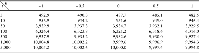
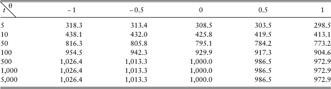
Tables 1 and 2 give the expected values
 $${\Bbb E}\left[ {Z_{t} } \right]$$
and standard deviations SD[Z
t
] of discounted aggregate claims Z
t
. The following two observations could be made.
1. For a fixed θ,
$${\Bbb E}\left[ {Z_{t} } \right]$$
and SD[Z
t
] are increasing with time t. As the duration of policy gets longer, it is reasonable to expect more claims.2. For a fixed t,
$${\Bbb E}\left[ {Z_{t} } \right]$$
and SD[Z
t
] are decreasing functions of θ. This is intuitive for SD[Z
t
] but not for
$${\Bbb E}\left[ {Z_{t} } \right]$$
as we expect, at least,
$${\Bbb E}\left[ {Z_{t} } \right]$$
is increasing when the dependence structure between claim severity and claim frequency is changing from negative to positive. However, this view is supported in a few references and interested readers may refer to Woo & Cheung (Reference Woo and Cheung2013), Cossette et al. (Reference Cossette, Marceau and Marri2008) and Chadjiconstantinidis & Vrontos (Reference Chadjiconstantinidis and Vrontos2014) for more details. It might be more explainable by writing down the equation and applying Theorem 3, from which we will end with


 $${\Bbb E}\left[ {Z_{t} } \right]\;{\equals}\;10000\left( {1{\minus}{\rm e}^{{{\minus}0.01t}} } \right){\minus}5.23240\theta {\plus}11.73404{\rm e}^{{{\minus}2.51t}} \theta {\minus}6.50164{\rm e}^{{{\minus}1.51t}} \theta $$
 $${\Bbb E}\left[ {Z_{t} } \right]$$
.

SD[Z t ].

The exponential functions vanish when t tends to infinity and therefore we can see that positive θ leads to lower expectations.
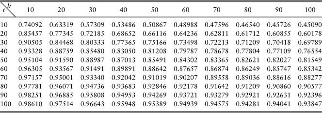
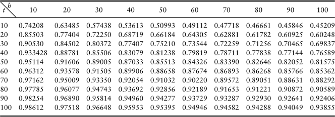
For correlation, in order to see the relationship between Z t and Z t+h , we take time t and step h starting from 10 with gap 10 as shown in Tables 3 and 4.
ρ(Z t, Z t+h ), θ=0.5.

ρ(Z t , Z t+h ), θ=−0.5.

The following observations can be made from Tables 3 and 4.
1. For all time t, step h and θ, Z t and Z t+h are positively correlated as expected, because Z t is part of Z t+h .
2. For a fixed time t and a fixed θ, ρ decreases as step h increases. This is intuitively reasonable as we expect risk profiles of one policy to become more distinct when time shifts.
3. For a fixed θ, step h has greater impacts when time t is small than when t is large.
Up to now, under this topic, results are easier to be achieved under time t infinity cases rather than for any t as one parameter is gone under infinity cases. Therefore our intention for these correlations is to see whether it is possible to give insights to any time t if we know the time infinity cases. However, above tables show it is not an ideal choice as the correlation of Z t is not good enough between small t and large t. In any case, ρ may not be a good choice as Z t may not be correlated with Z t+h in a linear form.
6. Explicit Results Under Gamma(2, λ ) Process
This section aims to show that the Beta transform is also applicable for other arrival processes. We will focus on the case where the inter-arrival times follow the Gamma(2, λ) distribution. For the Beta transform of a Gamma(2, λ) variable, see Example 3.
By Theorem 3 and taking the Laplace transform with respect to time t on both sides, we have
 $$\eqalignno{ {\cal L}_{r} \left\{ {V_{n} (t)} \right\}\;{\equals}\; & \mathop{\sum}\limits_{j\;{\equals}\;1}^n {\left( {\matrix{ n \hfill \cr j \hfill \cr } } \right){\Bbb E}\left[ {X^{j} } \right]{\cal L}_{r} \left\{ {V_{{n{\minus}j}} (t)} \right\}{\cal L}_{r} \left\{ {{\rm e}^{{{\minus}n\delta t}} {\lambda \over 2}\left( {1{\minus}{\rm e}^{{{\minus}2\lambda t}} } \right)} \right\}} \cr & \quad{\plus}\theta c{{{\rm \Gamma }(a){\rm \Gamma }(1{\plus}b)} \over {{\rm \Gamma }(a{\plus}b)}}\mathop{\sum}\limits_{j\;{\equals}\;1}^n {\left( {\matrix{ n \hfill \cr j \hfill \cr } } \right)\left( {{\Bbb E}\left[ {X_{{(a,b{\plus}1)}}^{j} } \right]{\minus}{\Bbb E}\left[ {X_{{(a,b)}}^{j} } \right]} \right){\cal L}_{r} \left\{ {V_{{n{\minus}j}} (t)} \right\}} \cr & \quad{\times}{{{\cal L}_{r} \left\{ {{\rm e}^{{{\minus}n\delta t}} F_{W} (t)^{{c{\minus}1}} \left( {1{\minus}F_{W} (t)} \right)^{d} f_{W} (t)} \right\}} \over {1{\minus}{\cal L}_{r} \left\{ {{\rm e}^{{{\minus}n\delta t}} f_{W} (t)} \right\}}} \cr & \quad{\minus}\theta d{{{\rm \Gamma }(a){\rm \Gamma }(1{\plus}b)} \over {{\rm \Gamma }(a{\plus}b)}}\mathop{\sum}\limits_{j\;{\equals}\;1}^n {\left( {\matrix{ n \hfill \cr j \hfill \cr } } \right)\left( {{\Bbb E}\left[ {X_{{(a,b{\plus}1)}}^{j} } \right]{\minus}{\Bbb E}\left[ {X_{{(a,b)}}^{j} } \right]} \right){\cal L}_{r} \left\{ {V_{{n{\minus}j}} (t)} \right\}} \cr & \quad{\times}{{{\cal L}_{r} \left\{ {{\rm e}^{{{\minus}n\delta t}} F_{W} (t)^{c} \left( {1{\minus}F_{W} (t)} \right)^{{d{\minus}1}} f_{W} (t)} \right\}} \over {1{\minus}{\cal L}_{r} \left\{ {{\rm e}^{{{\minus}n\delta t}} f_{W} (t)} \right\}}} $$
The key point is whether we are able to invert the fractional part involving f W (t). The calculation of the denominator is straightforward and the numerator part can be done in the following way.
 $$\eqalignno{ & {\cal L}_{r} \left\{ {{\rm e}^{{{\minus}n\delta t}} F_{W} (t)^{{c{\minus}1}} \left( {1{\minus}F_{W} (t)} \right)^{d} f_{W} (t)} \right\} \;{\equals}\;\mathop{\int}\limits_0^\infty {{\rm e}^{{{\minus}rt}} {\rm e}^{{{\minus}n\delta t}} \left( {1{\minus}e^{{{\minus}t\lambda }} (1{\plus}t\lambda )} \right)^{{c{\minus}1}} \left( {{\rm e}^{{{\minus}t\lambda }} (1{\plus}t\lambda )} \right)^{d} {{\lambda ^{2} } \over {\Gamma (2)}}te^{{{\minus}\lambda t}} dt} \cr & \quad \;\hskip144pt{\equals}\;\mathop{\sum}\limits_{k\;{\equals}\;0}^\infty {{{(1{\minus}c)_{k} } \over {k\,!\,}}\mathop{\int}\limits_0^\infty {{\rm e}^{{{\minus}rt}} {\rm e}^{{{\minus}n\delta t}} \left( {{\rm e}^{{{\minus}t\lambda }} (1{\plus}t\lambda )} \right)^{{d{\plus}k}} \lambda ^{2} te^{{{\minus}\lambda t}} dt} } \cr & \quad \;\hskip145pt{\equals}\;\mathop{\sum}\limits_{k\;{\equals}\;0}^\infty {{{(1{\minus}c)_{k} } \over {k\,!\,}}\mathop{\int}\limits_0^\infty {{\rm e}^{{{\minus}t(r{\plus}n\delta {\plus}(d{\plus}k{\plus}1)\lambda )}} t\lambda ^{2} (1{\plus}t\lambda )^{{d{\plus}k}} dt} } $$
where we apply Bromwich & MacRobert (Reference Bromwich and MacRobert1947: 151) to exchange the order of summation and integration. Further, when d is an integer, we can apply the Binomial theorem and see that
 $$\eqalignno{ {\cal L}_{r} \left\{ {V_{n} (t)} \right\}\;{\equals}\; & \mathop{\sum}\limits_{j\;{\equals}\;1}^n {\left( {\matrix{ n \hfill \cr j \hfill \cr } } \right){\Bbb E}\left[ {X^{j} } \right]{\cal L}_{r} \left\{ {V_{{n{\minus}j}} (t)} \right\}{\cal L}_{r} \left\{ {{\rm e}^{{{\minus}n\delta t}} {\lambda \over 2}\left( {1{\minus}{\rm e}^{{{\minus}2\lambda t}} } \right)} \right\}} \cr & \quad{\plus}\theta c{{\Gamma (a)\Gamma (1{\plus}b)} \over {\Gamma (a{\plus}b)}}\mathop{\sum}\limits_{j\;{\equals}\;1}^n {\left( {\matrix{ n \hfill \cr j \hfill \cr } } \right)\left( {{\Bbb E}\left[ {X_{{(a,b{\plus}1)}}^{j} } \right]{\minus}{\Bbb E}\left[ {X_{{(a,b)}}^{j} } \right]} \right){\cal L}_{r} \left\{ {V_{{n{\minus}j}} (t)} \right\}\mathop \sum\limits_{k\;{\equals}\;0}^\infty {{(1{\minus}c)_{k} } \over {k\,!\,}}} \cr & \quad{\times}\left\{ {\mathop{\sum}\limits_{i\;{\equals}\;0}^{d{\plus}k} {\left( {\matrix{ {d{\plus}k} \cr i \cr } } \right)\Gamma (2{\plus}i){{\lambda ^{{2{\plus}i}} } \over {(r{\plus}n\delta {\plus}(1{\plus}d{\plus}k)\lambda )^{{2{\plus}i}} }}{{(r{\plus}n\delta {\plus}\lambda )^{2} } \over {(r{\plus}n\delta )(r{\plus}n\delta {\plus}2\lambda )}}} } \right\} \cr & \quad{\minus}\theta d{{\Gamma (a)\Gamma (1{\plus}b)} \over {\Gamma (a{\plus}b)}}\mathop{\sum}\limits_{j\;{\equals}\;1}^n {\left( {\matrix{ n \hfill \cr j \hfill \cr } } \right)\left( {{\Bbb E}\left[ {X_{{(a,b{\plus}1)}}^{j} } \right]{\minus}{\Bbb E}\left[ {X_{{(a,b)}}^{j} } \right]} \right){\cal L}_{r} \left\{ {V_{{n{\minus}j}} (t)} \right\}\mathop{\sum}\limits_{k\;{\equals}\;0}^\infty {{{({\minus}c)_{k} } \over {k\,!\,}}} } \cr & \quad{\times}\left\{ {\mathop{\sum}\limits_{i\;{\equals}\;0}^{d{\minus}1{\plus}k} {\left( {\matrix{ {d{\minus}1{\plus}k} \cr i \cr } } \right)\Gamma (2{\plus}i){{\lambda ^{{2{\plus}i}} } \over {(r{\plus}n\delta {\plus}(d{\plus}k)\lambda )^{{2{\plus}i}} }}{{(r{\plus}n\delta {\plus}\lambda )^{2} } \over {(r{\plus}n\delta )(r{\plus}n\delta {\plus}2\lambda )}}} } \right\} $$
There are different ways to invert this Laplace transform by manipulating with the expression.
Theorem 7. For any δ≥0 and n, d∈ℕ, a recursive formula for the nth moment of Z t is
 $$\eqalignno{ V_{n} (t)\;{\equals}\; & {\lambda \over 2}\mathop \sum\limits_{j\;{\equals}\;1}^n \left( {\matrix{ n \hfill \cr j \hfill \cr } } \right){\Bbb E}\left[ {X^{j} } \right]\mathop{\int}\limits_0^t {{\rm e}^{{{\minus}n\delta v}} \left( {1{\minus}{\rm e}^{{{\minus}2\lambda v}} } \right)V_{{n{\minus}j}} (t{\minus}v)dv} \cr & {\plus}\theta c\lambda {{{\rm \Gamma }(a){\rm \Gamma }(1{\plus}b)} \over {{\rm \Gamma }(a{\plus}b)}}\mathop{\sum}\limits_{j\;{\equals}\;1}^n {\left( {\matrix{ n \hfill \cr j \hfill \cr } } \right)\left( {{\Bbb E}\left[ {X_{{(a,\;b{\plus}1)}}^{j} } \right]{\minus}{\Bbb E}\left[ {X_{{(a,\;b)}}^{j} } \right]} \right)} \mathop{\sum}\limits_{k\;{\equals}\;0}^\infty {{{(1{\minus}c)_{k} } \over {k\,!\,}}} \cr & {\times}\mathop{\sum}\limits_{i\;{\equals}\;0}^{d{\plus}k} {\left( {\matrix{ {d{\plus}k} \cr i \cr } } \right)} \mathop{\int}\limits_0^t {{\rm e}^{{{\minus}n\delta v}} g(v,d{\plus}1)V_{{n{\minus}j}} (t{\minus}v)dv} \cr & {\minus}\theta d\lambda {{{\rm \Gamma }(a){\rm \Gamma }(1{\plus}b)} \over {{\rm \Gamma }(a{\plus}b)}}\mathop{\sum}\limits_{j\;{\equals}\;1}^n {\left( {\matrix{ n \hfill \cr j \hfill \cr } } \right)\left( {{\Bbb E}\left[ {X_{{(a,\;b{\plus}1)}}^{j} } \right]{\minus}{\Bbb E}\left[ {X_{{(a,\;b)}}^{j} } \right]} \right)\mathop{\sum}\limits_{k\;{\equals}\;0}^\infty {{{({\minus}c)_{k} } \over {k\,!\,}}} } \cr & {\times}\mathop{\sum}\limits_{i\;{\equals}\;0}^{d{\minus}1{\plus}k} {\left( {\matrix{ {d{\minus}1{\plus}k} \cr i \cr } } \right)\mathop{\int}\limits_0^t {{\rm e}^{{{\minus}n\delta v}} {g}(v,d)V_{{n{\minus}j}} (t{\minus}v)dv} } $$
where
 $$\eqalignno{ g(v,\,d)\;{\equals}\; & \mathop{\int}\limits_0^v {\left[ {(1{\plus}i){\rm e}^{{{\minus}u(d{\plus}k)\lambda }} u^{i} \lambda ^{{1{\plus}i}} {\minus}(d{\plus}k){\rm e}^{{{\minus}u(d{\plus}k)\lambda }} u^{{1{\plus}i}} \lambda ^{{2{\plus}i}} } \right]} \cr & {\times}\left[ {{3 \over 4}{\plus}{1 \over 4}{\rm e}^{{{\minus}(v{\minus}u)2\lambda }} {\plus}{1 \over 2}(v{\minus}u)\lambda } \right]du \cr \;{\equals}\; & {3 \over 4}{\rm e}^{{{\minus}(d{\plus}k)v\lambda }} v^{{1{\plus}i}} \lambda ^{{1{\plus}i}} {\minus}{{{\rm e}^{{{\minus}2v\lambda }} } \over {4(d{\plus}k{\minus}2)^{{2{\plus}i}} }}\left[ {2{\rm \Gamma }(2{\plus}i){\plus}(1{\plus}i)(d{\plus}k{\minus}2)} \right. \cr & \left. {{\times}{\rm \Gamma }\left( {(d{\plus}k{\minus}2)v\lambda ,1{\plus}i} \right){\minus}(d{\plus}k){\rm \Gamma }\left( {(d{\plus}k{\minus}2)v\lambda ,2{\plus}i} \right)} \right] \cr & {\plus}{1 \over {2(d{\plus}k)^{{2{\plus}i}} }}\left[ {{\rm \Gamma }(2{\plus}i){\minus}{\rm e}^{{{\minus}(d{\plus}k)v\lambda }} \left( {(d{\plus}k)v\lambda } \right)^{{1{\plus}i}} {\minus}(1{\plus}i){\rm \Gamma }\left( {(d{\plus}k)v\lambda ,1{\plus}i} \right)} \right] $$
and
 $$\Gamma (z{;}\,\,\alpha )\;{\equals}\;{\int}_z^\infty {x^{{\alpha {\minus}1}} {\rm e}^{{{\minus}x}} dx} $$
is the upper incomplete gamma function.
Remarks
1. Equation (6.1) is computationally tractable and gives an explicit expression for V n (t), in particular for small n, can be obtained by further simplifying the integrals involved, as g(v, d) is essentially a linear combination of functions of type
$v^{\gamma } {\rm e}^{{{\minus}\xi v}} $
.2. Due to page limit, we choose not to include a numerical example for equation (6.1).

7. Concluding Remarks
This paper studies the moments and covariance of the discounted aggregate claims under a renewal risk model with dependence between the inter-claim times and claim amounts. The dependence is given by a generalised FGM copula which has four parameters with more flexibilities in dependence modelling. According to the structure of this copula, it is natural to define the Beta transform so that the main results can be expressed in terms of the Beta transforms of both claim amount distribution and inter-claim time distribution. This transform has many nice properties and some stochastic ordering properties can be used to derive upper and lower bounds for the moments of the discounted aggregate claims.
The Beta transform, with many nice properties, is demonstrated to be an efficient weapon in analysing quantities arising in risk models with the dependency being measured by the generalised FGM copula. It is believed that the Beta transform and its properties may have other applications in risk modelling and risk managements.
Acknowledgements
The authors would like to thank two anonymous referees for their valuable comments and suggestions which lead to significant improvement of the paper.