




No CrossRef data available.
DENSITY FUNCTIONALS, WITH AN OPTION-PRICING APPLICATION
Published online by Cambridge University Press: 04 August 2003
Abstract
We present a method of estimating density-related functionals, without prior knowledge of the density's functional form. The approach revolves around the specification of an explicit formula for a new class of distributions that encompasses many of the known cases in statistics, including the normal, gamma, inverse gamma, and mixtures thereof. The functionals are based on a couple of hypergeometric functions. Their parameters can be estimated, and the estimates then reveal both the functional form of the density and the parameters that determine centering, scaling, etc. The function to be estimated always leads to a valid density, by design, namely, one that is nonnegative everywhere and integrates to 1. Unlike fully nonparametric methods, our approach can be applied to small datasets. To illustrate our methodology, we apply it to finding risk-neutral densities associated with different types of financial options. We show how our approach fits the data uniformly very well. We also find that our estimated densities' functional forms vary over the dataset, so that existing parametric methods will not do uniformly well.We thank Hans-Jürg Büttler, Aleš Černý, Tony Culyer, Les Godfrey, David Hendry, Sam Kotz, Steve Lawford, Peter Phillips, Bas Werker, and three anonymous referees for their comments. We also thank for their feedback the participants at the seminars and conferences where this paper has been invited, in particular the 1998 CEPR Finance Network Workshop, the 1998 METU conference, the 1998 FORC (Warwick) conference “Options: Recent Advances,” Money Macro & Finance Group, the Swiss National Bank, Imperial College, Tilburg University, Université Libre de Bruxelles, the University of Oxford, Southampton University, and UMIST. The first author acknowledges support from the ESRC (UK) grant R000239538. The second author acknowledges help from the HEC Foundation and the European Community TMR grant “Financial Market Efficiency and Economic Efficiency.” This paper was written when the second author was affiliated with HEC-Paris.
Information
- Type
- Research Article
- Information
- Copyright
- © 2003 Cambridge University Press
1. INTRODUCTION
It is often the case that one wishes to estimate a probability density function (p.d.f.) of a variate, without prior knowledge of its functional form. If the variate is directly observable, a number of parametric and nonparametric methods are already available for estimating the density. If, however, the variate is not observable, and its density can only be extracted indirectly, the problem is more complicated. In this paper, we propose a method that can be used in the case of either type of variate. Its advantages are illustrated with the following application.
1.1. A Motivating Problem
Let St be the price of an asset at time t. To illustrate, we assume for the moment that the asset does not pay dividends and that it is domestic, i.e., no considerations need to be paid to foreign interest rates. Later on, we will consider an extension to foreign currency options.
Suppose that this asset is underlying a European call option with expiration date T and strike price K. Then, the intrinsic value of this option at expiration is VT = max(ST − K,0). In an arbitrage-free economy, it is known (see Harrison and Pliska, 1981) that there exists a risk-neutral density (RND) g(·) such that the price of a call option can be written as

where Et(·) is the expectations operator conditional on all information available at time t, Ct(·) is the price at time t of the call option, and r is the continuously compounded risk-free interest rate. The function Ct(·) depends on the parameters r,T,t and also on others characterizing the process followed by St. In an arbitrage-free economy we also have the martingale condition

where the expectation is taken with respect to the RND g(·).
As noticed by Breeden and Litzenberger (1978), differentiating the integral gives

where G(·) is the cumulative distribution function (c.d.f.) corresponding to the p.d.f. g(·). The second derivative is given by

which reveals the required density g(·). It is convenient to work with the future value

whose second derivative is the required density function.
If the asset were to return a yield of r*, or if we were to consider a currency call option with foreign interest rate r*, the martingale condition of the arbitrage-free economy (2) would be

instead of (2). Of course, no alterations are necessary in formulas (1), (3), and (4), where r is the unchanged discount factor used to calculate present values.
One way to estimate the density is to postulate a parametric form for g(·), work out analytically the corresponding integrals leading to an explicit C(·), and then fit the observed option prices C(K) to the strike prices K to determine the parameters of g(·). Mixtures of lognormal distributions have been used by Bahra (1996), Melick and Thomas (1997), and Söderlind and Svensson (1997). It is possible to assume that the underlying process is more general than a lognormal diffusion (for jump-diffusion versions, see Bates, 1996a, 1996b; Malz, 1996).
Alternatively, a nonparametric approach may be adopted. Jarrow and Rudd (1982) have developed a method based on an Edgeworth expansion involving a lognormal density. This approach has been implemented by Corrado and Su (1996) to price options. Using a system of Hermite polynomials, Madan and Milne (1994) suggest a method of approximating the underlying RND, and Abken, Madan, and Ramamurtie (1996) provide an application. See also Knight and Satchell (1997) and Jondeau and Rockinger (2001), where Gram–Charlier expansions are used. Stutzer (1996) uses a Bayesian method based on the maximum-entropy principle of Shannon. Finally, in a time series context where large datasets are available, Aït-Sahalia and Lo (1998) fit kernel-based estimates to the RND. See also Bondarenko (2000). For a survey assessing existing methods, see Jondeau and Rockinger (2000). Also, numerical methods can be used to estimate functionals of densities and/or to simulate option prices, but these have not been used to generate RNDs (e.g., see Wilmott, Dewynne, and Howison, 1993).
Improvements over these approaches are possible, because they are either restrictive (lognormals or jump-diffusions), do not always yield positive probabilities (Edgeworth expansions or Hermite polynomials), or require a large number of observations (kernel estimates). Furthermore, the methodology we are about to suggest is general, and it may be applied to other problems not necessarily related to finance or economics.
1.2. The Plan
The initial problem is to design a general function whose second derivative is a class of density functions. We derive such a function, and find that it is based on the confluent hypergeometric 1F1 function.1
There are two different types of confluent hypergeometric functions, Kummer's 1F1 and Tricomi's Ψ (see Abadir, 1999, and references therein). There are also two related confluent hypergeometric functions due to Whittaker, M and W. We use only 1F1 in this paper.
For practical purposes, parsimony of the model is important. For example, considering the data in our motivating problem, there are not many strike prices available. Our approach is of a parsimonious semi-nonparametric nature, closest in spirit to fitting a system of orthogonal Hermite polynomials. However, we do not estimate a system but rather the parameters of a couple of functions. The functions we use include Laguerre and Hermite polynomials as special cases, with the added advantage that Abadir's (1993a, 1999) “fractional” polynomials allow for monotonic behavior at the tails of the density and thus do not suffer from the forced oscillatory nature that standard polynomials have for extreme values. Within our model, parameter estimates determine the functional form, in addition to the usual distributional properties (e.g., centering and scaling). This is more efficient than fully nonparametric estimation, which runs into difficulties in small samples. It is also more flexible than parametric methods that restrict functional forms.
We do not restrict the functional form of the density to a single type. The only restriction we impose is that it must belong to some family of densities to be specified in Section 2, which includes exponential and degenerate nonexponential cases. This new class of closed-form densities that we are proposing can have applications in other areas of statistics too and can be used to characterize a broad selection of continuous random variables. For example, this class can be used to provide an alternative approach to fully nonparametric density estimation. Another application would be to model nonnormal densities in generalized autoregressive conditional heteroskedasticity (GARCH) models, etc. Our class of densities does not assume the existence of moments, thus avoiding the problem of basing an estimation procedure on calculated “moments” that may be spurious.
In the next section we introduce our density functional, based on 1F1, for the case of double integrals of densities. In Section 3 we illustrate this methodology with two applications in option pricing. We also discuss how the empirical findings can be used for practical purposes. In Section 4, we generalize the methodology to the case of observing any functional (not necessarily double integrals) of densities. We conclude in Section 5. Proofs and lengthy derivations are collected in the Appendix.
We denote the set of natural numbers (which excludes zero) by

and real numbers by

. The indicator function is written as

, returning 1 if condition

is satisfied and 0 otherwise. The (complete) gamma function is denoted by Γ(ν) for

, and defining

leads to the generalized hypergeometric function

where

. Special cases that we will be discussing frequently are


where γ(·,·) is the incomplete-gamma function, Φ(z) is the standard normal c.d.f., and sgn(z) is the sign function.
2. THE DESIGN OF DENSITY FUNCTIONALS
The 1F1 function can represent a variety of density-related functions, and we will use it in Section 2.1 to propose a generalization of the normal, gamma, and other variates. We will briefly outline how our functional is constructed and how it reduces to some well-known continuous random variables in statistics. Sections 2.2 and 2.3 derive, respectively, the restrictions necessary for the density functional to have a proper underlying density and the moments implied by this function. Section 2.4 discusses strategies for the estimation of our function.
2.1. Specification and Main Special Cases
We need to model integrals of c.d.f.s and possibly mixtures (integrals) thereof. Integrating n times the functions γ(ν,z) of (6)

and Φ(z) of (7)

The latter is obtained by means of the parabolic cylinder function (see Abadir, 1993b, 1999), and integrals of negative orders (i.e., derivatives) yield the well-known Hermite polynomials. Generally, parabolic cylinder functions are linear combinations of 1F1 functions that would allow for fractional n in (9) and are closed under differentiation and integration: these operations keep the result within the same class of functions. A weaker version of this property applies to other linear combinations of 1F1 too, and this makes them appealing in modeling an arbitrary number of functionals of a class of densities that encompasses the normal, gamma, and others. We defer introducing the case of an arbitrary number of functionals until later in Section 4, because of the added level of difficulty that it poses.
For double integrals of densities, a mixture that extends the cases seen earlier is given by

where

. The indicator function is required to represent a component of the density with bounded support. It is also sufficient for keeping the function real-valued for general b1 and b3.
Not all the parameters in C(·) are free to vary unrelatedly, because some restrictions (at least three in general and at least seven in our motivating example) are needed for the function to be the integral of a c.d.f., and we shall analyze these restrictions in detail in our next section. Now, we analyze the relation of C(·) to familiar distributions.
The first two parameters, c1 and c2, drop out when differentiating twice to get the density, but they are needed in general either to represent the constants of indefinite integration or when one of the limits of definite integration is infinite. An example of the need for such constants is in (3), where the integral of the density is over (K,∞) rather than, say, (−∞,K). If the limits of integration of the functional are an interval that is a strict subset of the support of the density, then one would end up with the difference of two C(·) functions. We shall not consider this case explicitly, because it boils down to using C(·) twice.
The first 1F1 function in C(·) covers the gamma and other asymmetric generalizations, whereas the second covers the case of symmetric quadratic-exponentials such as the normal. We do not go further to quartic-exponentials (or higher powers of even order) because they are unlikely to occur in practice unless the variate is almost degenerate. They are nevertheless covered approximately by b3 in the first 1F1 function. Examples of special cases giving integrals of known density functions include

where standardization (e.g., centering around zero) is not imposed and the constants of integration c1 and c2 are to be determined by the problem at hand. For the listing of the normal, recall that the first term in (9) reduces to z/2 when n = 1. Extreme-value distributions are useful in the field of value-at-risk in finance, and they are a special case of our approach. For further degenerate special cases, see the discussion of confluences in Abadir (1999).2
The function can also mimic the basic properties of a lognormal. For this, use page 68 of Abramowitz and Stegun (1972): the leading term is picked up by the symmetric quadratic component (latter one) of C(·), whereas the asymmetry is represented by the rest. See also Johnson et al. (1994, 1995) for approximating the lognormal density by normal, gamma, and/or Weibull ones.

obtained from the expansion in (5). This is a case where the existence of higher order moments will hinge on the magnitude of a2. By the definition of the Pareto density, we require in addition that a2 ∈ (−1,∞) and

. When estimating the function C(·), it is worth testing for its reduction to known simpler cases such as those outlined previously and others in Johnson, Kotz, and Balakrishnan (1994, 1995).
Given the fact that our method encompasses a large class of traditional densities and is flexible, we believe that the potential for misspecification is small. Of course, misspecification is always a possibility, even with the most flexible of methods that assume the least (e.g., fully nonparametric methods). For example, let ζ and ξ be two independent standard normal variates. Then, the product η ≡ ζξ has a density that is infinite at the origin and that could be represented by hypergeometric functions of the sort we use (see Abadir, 1999, p. 302). If one were to fit a nonparametric density to data generated for η, then the kernels would smooth (build a “bridge”) over the origin in spite of the true density being discontinuous there. Our method avoids such assumptions and encompasses a broad class of statistical densities, including ones with discontinuities.
2.2. Necessary Restrictions on the Parameter Space
The second derivative of the C(·) function is a mixture of the densities mentioned earlier. By differentiating termwise the 1F1 series,

The estimate of g(z) that is implied from the estimate of C(z) should be a density. It should be nonnegative over its support, say,

, and integrate to 1.
The nonnegativity restriction is hardly ever binding near the optimum parameter estimates, given the design of our function C(·). Nevertheless, it can be imposed on the estimation routine by a Lagrangian penalty function involving min(0,g(z)), if the optimum g(·) is found to be negative. We did not need to do so in our applications.
For the restriction on the integral of the density, we derive

This expression is linear in, at least, c2 and a4 so that the two restrictions that ensure the proper choice of constants of integration, namely,

give rise to an explicit constraint on each of c2 and a4. These can be directly substituted into our C(z) and there are two fewer parameters to estimate. The two restrictions will be illustrated in the Appendix.
We have mentioned restrictions on the p.d.f. (positivity) and then two more on the c.d.f. It is also natural that the integral of the c.d.f. will necessitate one more restriction, namely, one to do with the constant of integration, which is application-specific. It takes the form of a boundary condition on C(·), e.g., C(∞) equals some fixed value. Such conditions are often known in economics (especially in growth theory) as transversality conditions and will be illustrated in the Appendix. Because C(·) is linear in c1, this condition implies an explicit restriction on c1 that can be substituted directly into our function C(z).
2.3. Explicit Characterization of the Moments
Finally, it is useful to characterize the moments of the density. One of the reasons for doing so could be the desire to investigate and/or impose restrictions on the moments of the density if some theory (e.g., arbitrage pricing theory) requires them. Another reason may be the desire to estimate our function C(·) by fitting the data to its analytical moments, which is discussed later in Section 2.4.
Subject to these functions being nondegenerate (i.e., the existence condition for the moments),

by integrating by parts two times. For n = 1 and assuming m1 ∈ (z[ell ],zu), this gives

by substituting from (13) and (10), respectively. This expression is linear in a1 and can be used to reduce further the number of parameters to estimate, if there are reasons to believe that E(z) needs to be restricted, e.g., as a result of the no-arbitrage condition (2) in our example. This, along with a simplification of the expression, will be done in the Appendix.
For n > 1, (14) requires us to work out an explicit formula for the integral. Substituting for C(z) from (10) and integrating termwise,

Asymptotic expansions of p Fq can be used to simplify the expression further, for extreme values of z[ell ] or zu, as is illustrated in the Appendix.
2.4. Strategies for Estimation and Inference
There is more than one possible method for estimating our function C(·). These include maximum likelihood (ML), generalized least squares (GLS), generalized method of moments (GMM), and other approaches. We only discuss these three. Other attractive estimation methods, such as M-estimators, can be analyzed in the same way if desired.
The pseudo-likelihood approach is one of the most appealing. In the simplest case where the errors of estimating our functional C(·) are spherical normals, we can fit the functional to the observed data by nonlinear least squares (LS). In general, however, the errors may be nonspherically distributed. If there was evidence of nonspherical errors, one could specify a covariance structure for the residuals. Keeping the assumption of a pseudo-Gaussian likelihood, one could then estimate the variance-covariance matrix, say, Ω, by an iterative (e.g., two-step) procedure. An analogous idea would apply to GLS estimation, albeit with a difference of a factor of ½log(det(Ω)) for the objective function to be optimized.
Another potentially appealing approach would rely on the explicit formulas for the moments, which we have derived in the previous section. GMM estimation would be based on these expressions. However, we have an important concern with applying this method here. We would only recommend it if the user were willing to restrict estimation to a class of our underlying densities where the moments do exist. We have given an example of our class of densities, the Pareto, where some moments do not necessarily exist. Subject to this proviso, the appeal of GMM would be in the ease of obtaining an estimate of the covariance matrix for the moment restrictions.
Two theorems will now be derived for the case of a random sampling of N observed values of C(z) and the nonlinear LS estimation of the model

where estimates are denoted by a hat, ε has zero mean and variance ω2 < ∞. The conditions on ε are sufficient but not necessary for the theorems to hold. Moreover, when the sampling scheme is not independent and identically distributed (i.i.d.) then, for the theorems to be valid, we assume that the other methods of estimation discussed earlier are used with the correct covariance structure. Let θ denote the vector of parameters of the function C(z), which are defined in (10) subject to the (exclusion) restrictions outlined there and which we denote by θ ∈ Θ. Then, we have the following result.
THEOREM 1. The nonlinear LS estimators of θ ∈ Θ are consistent for any of the parameters that have a nonzero impact on the function C(z).
The last part of the theorem's statement refers to the situation when some component of C(z) drops out, in which case some (irrelevant) parameters will not be estimated consistently. For example, if a1 = 0, the parameters m1,a2,a3,b1,b2,b3 in (10) are neither identified nor estimated consistently. In such cases, however, these parameters have no effect at all on C(z) and are of no interest.
We now turn to inference regarding the estimated parameters. For this, we restrict θ ∈ Θ further to

by excluding the cases where either of a1,a2,b2,a5 is zero,
3The parameter a4 is not free to vary unrestrictedly (see the discussion of (13)). To some extent, m2 is also not free to vary, if one believes in arbitrage pricing (see (15) or more clearly (17)).
THEOREM 2. The nonlinear LS estimators of

are asymptotically normal with mean θ and covariance matrix

where N is the sample size.
We need to qualify inferences in our applications of the next section with a warning, because small datasets are involved and asymptotic inference may be of limited relevance there. The issue of finite-sample inference within a general context is, as ever, an unresolved problem. Various possibilities for attempting to improve such inference exist, but we do not pursue them in this paper, and we rely instead on the well-documented robustness of F-tests (but not of t-ratios) (e.g., see Ali and Sharma, 1996; Godfrey and Orme, 2001; and their reference lists). Examples that can help improve finite-sample performance include resampling methods such as the bootstrap. The difficulties with bootstrapping in the current setup are that it would be computationally very expensive and that establishing analytically its validity for 1F1 functions is beyond the scope of this paper. For examples on the inconsistency of the bootstrap, see Basawa, Mallik, McCormick, Reeves, and Taylor (1991), Young (1994), and Andrews (2000). Of particular relevance is the discussion in Young (1994, especially p. 385) about its failure in environments where moments need not exist (e.g., stable laws), which can be the case when our function collapses to the Pareto density (11).
3. APPLICATIONS TO OPTION PRICING AND RISK-NEUTRAL DENSITIES
3.1. The Empirical Setup
We illustrate our methodology with foreign exchange options and with S&P500 index options. Both types of options are known to exhibit deviations from lognormality and are likely to reveal an interesting pattern in terms of densities (for foreign exchange options, see Bates, 1996a, 1996b; for S&P500 options, see Rubinstein, 1994). Because our only goal in this part is to illustrate the usefulness of our method, rather than to describe of all available options, we represent the results for a few dates and maturities.
First, for foreign exchange data, we use over the counter (OTC) options. Even though there exist options listed on currency exchanges, the vast majority of currency options are traded in the OTC market. According to the Bank of International Settlement, in June 1999, the notional value of outstanding OTC currency derivatives was about 200 times larger than that of currency exchanges. This implies that foreign currency OTC markets have greater liquidity. The drawback is that OTC option prices are usually unavailable to the public. We were able to collect OTC data of European French franc/Deutsche mark (FF/DM) rate options, in addition to the current exchange rate, from a large French bank for one randomly selected date (17 May 1996) during which no particular event happened and also for another date occurring a few days after President Chirac announced a snap election (28 April 1997) that eventually led to a landslide victory of the then opposition party.
For a given time of the day, the bank that provided us with the data requested quotes from the other dealers in the market. Dealers are compelled to give a bid-ask quote. The bank then retained the best bid and ask quote for various strike prices. The fact that the bank retained dealer's quotations guarantees that the option prices are determined simultaneously. The situation would have been quite different if only prices for traded options were available. In such a situation reported prices might have been obtained at very different times of the day, possibly, for very different values of the underlying asset, in which case prices would have been stale. Also, for many strike prices there may not have been transactions. Similarly, we were given the exchange rate from the same source. For exchange-rate quotes, the mechanism is similar to OTC options in that dealers must quote a bid and ask price. This means that for the foreign currency options, the magnitude of the nonsynchronicity bias is small. The drawbacks of this market are that prices are not publicly available and that we were able to obtain data only for a few days.
For the first and second dates, we were able to obtain the bid and ask prices for options corresponding to (N =) 13 and 11 different strike prices, respectively. Even though one could, for the purpose of option pricing, compute RNDs for the bid or the ask side, we decided to follow initially the convention of using the average of the bid and ask price for each strike price. Taking the mid-spread is compatible with the use made by central bankers, who are mainly interested in the evolution of the density and its shape (e.g., see Campa, Chang, and Reider, 1997). Nevertheless, we check in Section 3.3 the importance of using the mid-spread rather than the bid or the ask prices. We report results on options with two different maturities, 1 and 3 months.
Second, for the S&P500 options, we downloaded the prefiltered data used and described in Aït-Sahalia and Lo (1998). The options are European, cover 1993, and for each date there are various maturities available. Unlike our foreign exchange options, these index options are characterized by many strikes and a high liquidity. We selected three dates randomly and chose a maturity with a large number of strikes.
The benchmark option pricing model assumes that the underlying asset's price process follows a lognormal diffusion with constant volatility σ. In this case, European-type call options are traditionally priced with

where

Similar formulas apply to put options. If r* is a foreign risk-free interest rate, then we obtain the Garman and Kohlhagen (1983) formula for foreign exchange options. If, instead, r* is the continuous dividend yield, then we obtain the formula for index options of Black and Scholes (1973) and Merton (1973). In the numerical applications for FF/DM options, we take for r and r* the domestic (French) and foreign (German) euro-interest rates chosen to match the expiration of the options. We obtain data on these rates and transform them into their continuously compounded equivalents.
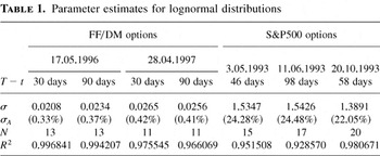
If one is willing to assume that volatility is constant across all strike prices, then it is possible to estimate the single volatility parameter σ2. We follow the literature in doing this by minimizing the quadratic distance between actual and fitted prices, i.e., by nonlinear LS. Table 1 presents the estimates of such volatilities and also the associated goodness of fit measures. For both dates of the FF/DM options, we notice a slightly better fit for the first maturity than for the second maturity. For the S&P500 options, we notice a better fit than for FF/DM options, with the fit being similar across the three dates.
Parameter estimates for lognormal distributions

The annualized volatility is denoted by σA2. For FF/DM, σA ranges between 0.33% for the 30 days-to-maturity options on 17 May 1996 up to 0.42% for similar options on 28 April 1997. These figures are slightly smaller than those reported by Malz (1996), who considers the DM/£ in 1992, a series that is known to behave more erratically than the FF/DM. The annualized volatility of the S&P 500 ranges between 22.05% for the option on 20 October 1993 to 24.48% for the option on 11 June 1993. The difference in magnitude between the volatilities of exchange rates and stock returns is large. However, the data are of very different nature, and the market structures also differ. For instance, the FF/DM market was subject to tight trading bands within the European Monetary System.
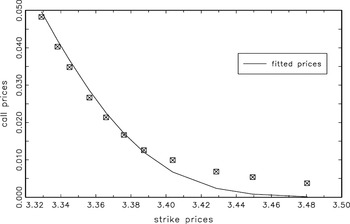
To get an overall feel for the inaccuracy of these benchmark fits, we present in Figure 1 a typical plot of actual and fitted prices taken from the 3-months to maturity options of 28 April 1997. We notice that, for options with a high strike price, the fit is bad. This implies that a model with constant volatility across different strike prices is incomplete. In other words, volatility is dependent on K (a phenomenon known as the volatility “smile” because of the U-shaped relation), and further information that is not extracted by the lognormal is contained in the available option prices. This further information can be captured with a hypergeometric-based RND, as we will show.

Original and fitted Garman–Kohlhagen call option prices, 28 April 1997, 3-months to maturity.
3.2. Numerical Aspects of Estimating Our Nonlinear Function C (·)
We performed all optimizations with the GAUSS program and the OPTMUM module. We used nonlinear LS as our fitting criterion for C(·), as we did with the lognormal. In general, though, one should consider other methods based on GLS or a likelihood criterion, as we have discussed in Section 2.4. We do not elaborate on this point in this section, given how uniformly good the fit turned out to be and given that the sample we have for the observed C(·) is random. This is because the data are given over a grid of options' “deltas,” the term for ∂C/∂S. This derivative is a constant plus the distribution function G(·) (e.g., see (A.2) in the Appendix). Because the distribution function of a continuous variate is uniformly distributed when the function's argument is random, taking a grid over the option's deltas is equivalent to stratified sampling.
In nonlinear estimation, it is crucial for numerical stability to obtain estimates of comparable magnitudes. To help the program find such estimates, we rescale the strike prices K by defining the linear transform z ≡ α + βK. Because C(·) is tied to the density of z, it is also necessary to rescale the option prices by the Jacobian of the transform, according to βC(K) = C(z). Because the bulk of standardized density masses tends to lie in the interval [−3,3], the mapping of strike prices achieving approximately z ∈ [−3,3] will yield a numerically stable estimation procedure.
Another important element in numerical optimization is the choice of initial values. The lognormal benchmark has a shape that is not too different from a normal. We therefore chose for the optimization to start with parameter values that arise from a normal RND. From the discussion following (10),

and the component starting with a1 is set to zero. Setting a1 = 0 initially does not guarantee a well-behaved function at the next iteration. For example, care should be taken not to let

, as a division by zero may occur in computing the 1F1 function (see the expansion in (5) and the subsequent exclusion restrictions). To make the program run smoothly, the starting values of the initially omitted component (the one beginning with a1) may be those of a restricted gamma, e.g.,

because of the shape of RNDs known to arise in the literature (see the references cited earlier).
We saw in Section 2.2 that explicit restrictions on c2, a4, and c1 exist and must be implemented in the estimation routine, and in the Appendix we simplify them for the setup of our problem. Additionally, we found in our numerical applications that the reductions implied by the joint hypothesis b1 = 1 + a2 b3, a5 = −½, a6 = ½ cannot be rejected by an F-test. This simplifies the former restrictions further to

as shown in the Appendix. Finally, for the no-arbitrage condition to be checked, (2) or (15) simplifies to

which is naturally a weighted average of m1 and m2. In both our applications, we found that the condition was satisfied by the data. We now summarize the empirical results.
3.3. Summary of the Results
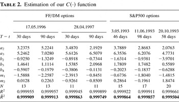
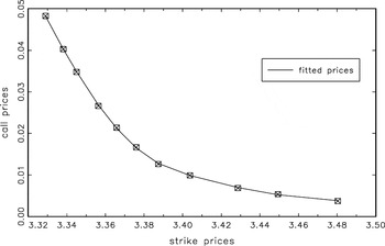
Following the estimation strategy outlined previously, we obtain the estimates displayed in Table 2 for the various dates and maturities. Because R2 is invariant to affine transformations of the data, a comparison of this statistic with the one in Table 1 is feasible. We notice that across all estimations, the R2 and the R2 adjusted for degrees of freedom (i.e., R2) for our fit are larger by a sizable magnitude than the ones obtained for the lognormal distribution. For DM/FF options we display in Figure 2 the plot of actual and fitted prices taken from 28 April 1997 (3-months maturity), which is representative of the fit at all the dates we tried. We notice an excellent fit for all options. Also, a direct computation of option prices involving formula (1) with a numerical routine corroborated that our method gives a very good fit.
Estimation of our C(·) function


Original data and hypergeometric-based fit, 28 April 1997, 3-months to maturity.
We obtain a discretization of the RND by evaluating g(·) over a grid consisting of 1,000 points, and the plot for two dates and two maturities is in Figures 3, 4, 5, and 6. The link between the RND and actual (or objective) probabilities involves the degree of risk aversion of investors, and an interpretation of the RND as if it concerned the probability of the financial asset belonging to a certain range is a rough approximation. Aït-Sahalia and Lo (2000) and also Jackwerth (2000) show how a measure of risk aversion may be inferred from RNDs and the actual probabilities. Conversely, if one had a model describing risk aversion one could make a statement about actual probabilities. These investigations are beyond the scope of our paper, and central bankers are typically more interested in how RNDs change from day to day than in measuring risk aversion.

Lognormal and hypergeometric-based risk-neutral densities, 17 May 1996, 1 month maturity.

Lognormal and hypergeometric-based risk-neutral densities, 17 May 1996, 3-months to maturity.

Lognormal and hypergeometric-based risk-neutral densities, 28 April 1997, 1 month maturity.

Lognormal and hypergeometric-based risk-neutral densities, 28 April 1997, 3-months to maturity.
Interesting comparative statics can be drawn from analyzing RNDs for different dates and/or maturities. The influence of major events is reflected in their changing shapes. In our first application, graphical inspection of the RNDs confirms that the first date was a rather quiet one, whereas the second date was amid a period of great agitation. Figures 3 and 4 display the RND for FF/DM options at 17 May 1996, for the two maturities. We notice that for the higher maturity the spread is much larger, translating the fact that market participants associate more uncertainty with the longer run. Also, in comparison with the lognormal case, we notice that our method reveals a heavier right tail. This translates the fact that investors, even on a rather normal day, are paying a premium in the anticipation of a latent devaluation of the FF (the so-called peso problem).
When we turn to the second date, there is an overall shift to the left for all distributions coming from the fact that, at that date, the FF had appreciated with respect to the DM. When we compare the distributions with those of the first date, there is a larger spread for the p.d.f. at all maturities. In other words, for the second date the global uncertainty is much larger. In addition, the right tail is more slowly decaying for the second date, reflecting the fact that market participants were contemplating the possibility of a large subsequent depreciation of the FF, with a nonnegligible probability.
It should be mentioned that the bimodality of the RND, which has arisen in the literature cited earlier, is also found to varying extents in Figures 3, 4, 5, and 6. In our function, we have not forced this bimodality (or any other oscillatory-tail features), as is clear from looking at our graphs. Our earlier talk of “two” components in our C(·) should not give the erroneous impression that our C(·) is based on just a mixture of two densities with at most two modes (see (12) for analytical details). Our graphs illustrate that this is not the case, some displaying multimodality but others not. See also the discussion after (A.8) in the Appendix, where we could not reduce our estimated functions to just mixtures of normal and gamma.
The multimodality, when it appears, could be due to a number of reasons. For exchange rates, the most plausible explanation of the right hump is the expectation of a widening of the target band. The center of the target zone was set at 3.35 FF/DM and the width was set at ±2.5%, implying a band ranging from 3.2746 up to 3.4254. The right hump, being outside this band, suggests that market participants put a nonnegligible probability on a devaluation of the FF with respect to the DM.
To check the robustness of our estimated RNDs, say,

, and the corresponding distributions

, we perform a sensitivity analysis. We estimate the parameters of the hypergeometric-based C(·) when omitting one different strike price at a time, obtaining N estimates of RNDs, each based on N − 1 strikes. Denote each of these estimated densities by

and their corresponding distributions by

, where j = 1,2,…N. To illustrate, we choose our “worst”-fitting C(·), namely, the FF/DM options at 28 April 1997, for the second maturity. We find that the maximal absolute deviation between

and each of the 11 c.d.f.s

, for any j or ST, is

which is about half a percentage point, thus indicating a very stable estimate of the c.d.f. This observation is corroborated by Figure 7. There, the dotted line represents our density estimate

, whereas the narrow band around it is obtained pointwise (i.e., for each ST) as the minimal and maximal value over the N estimates

. This indicates that our estimated RNDs are robust to a number of possible concerns raised in the finance literature, in addition to the traditional econometric ones. For example, our RNDs are robust to dropping the observation with the largest bid-ask spread, or the observation with the largest (or smallest) strike price K, etc.

Sensitivity bounds for the hypergeometric-based density with one strike deleted at a time.
We check further the robustness of the estimated shapes to bid-ask spreads, because this is a particularly important issue. To do so, we reestimate the densities by first assuming that all option prices were at the ask side and then by assuming that they were all on the bid side. We perform these estimations for 28 April 1997, a day when markets were rather agitated, and for the relatively illiquid 3 months to maturity option. For these options, the spreads tend to be the largest of all the options considered in this study. The results of the estimation are displayed in Figure 8. As can be seen, the overall shape of the densities is the same. In particular, the bimodality of the RNDs for this date appears to be numerically stable and not simply due to an error in the data. Considering the implied c.d.f.s, we find that the maximal discrepancy between the mid-spread and the bid-only (respectively, ask-only) prices is 0.058 (respectively, 0.047). Though the shapes are analogous, the discrepancy of roughly 5% is larger than the one found in (18) because here we take the sensitivity analysis to the extreme of changing all prices simultaneously. Even so, the maximal discrepancy between the distributions occurs very close to the peak (first mode) of the density, namely, at 3.37 and 3.35, respectively, but not in its tails, which are of most interest as explained earlier in connection with Central Bank policy-making.

Hypergeometric-based estimated densities with ask, with bid, and with mid-spread option prices.
We now turn to the estimation results pertaining to fitting our C(·) function to the S&P500 options. Inspection of the second part of Table 2 confirms our earlier results: the hypergeometric-based C(·) function allows for a very close fit, of comparable quality to the one obtained for the FF/DM options. For 3 May 1993, Figure 9 represents the RND obtained with the lognormal model and the hypergeometric one. We notice now, in line with the figures represented in Aït-Sahalia and Lo (1998), that the RND is negatively skewed for Index options. This pattern translates the idea that investors fear a crash. A lognormal cannot represent a negatively skewed density, and thus seems to be incompatible with the data, whereas our hypergeometric-based densities allow for either type of skewness.

Lognormal and hypergeometric-based risk-neutral densities, S&P500 index options, 3 May 1993, 46-days to maturity.
Finally, we compare our results to the fits obtained by other methods. We do not fit the entropy-based model, because it has as many parameters as data points and is therefore going to lead to R2 = 1 and R2 = 0 everywhere. As for the others, Table 3 reports the results. The label “Hermite” refers to the method used by Jondeau and Rockinger (2001) to enforce nonnegativity constraints on the estimation of Gram–Charlier densities by means of Hermite polynomials. “Jumps” refers to the Malz-type jump-diffusion model discussed in the introduction, whereas “Mixtures” is the generalization of the benchmark into lognormal mixtures. It is clear from the table that our method is always best in terms of R2 and is only once beaten by “Jumps” in terms of an R2 that differs from ours by less than a unit in the fifth decimal place! Our method does very well and uniformly so for
(1) volatile days, in addition to quiet ones;
(2) different maturities; and
(3) options on very different underlying assets.
Our estimated densities' functional forms vary over the dates and maturities, as can be seen in Table 2 from the parameter estimates of a2,a3,b3, the other parameters playing mainly centering and scaling roles. Therefore, parametric methods that restrict functional forms (e.g., mixtures of lognormals) will not do uniformly well. Notice also that Table 2 indicates that, in all cases studied, the tails of the RNDs decay exponentially fast. For the markets studied, this implies that all moments of finite order exist and that the perceived probability of extreme events declines at exponential rates. The estimated parameters of the asymmetric component of (10) were such that it ended up representing extreme events by means of long tails, especially because b3 is mostly smaller than the exponential power 2 of the other component.
A comparison of R2 and R2 (in bold) for other methods

4. THE DENSITY FUNCTIONAL FOR REPEATED INTEGRALS
Section 2 gave a C(·) function based on generalizing (8) and (9) for the case of double-integrals of p.d.f.'s. Here, we extend this approach to the situation where the pth integral of a p.d.f. is observed, where p ∈

, by taking

The parameters are not generally (i.e., for p ≠ 2) in correspondence with our earlier C(z), but the modeling methodology is the same and so is the number of free parameters. The case p = 1 is one where the variate z is directly observable, and its empirical c.d.f. is available to compare to our fitted c.d.f. C(z).
Three types of restrictions on the parameters of C(z) are needed:

In this section, without a specific application in mind, one can only implement restrictions of Types IA (up to a constant) and IB and provide formulas (such as expressions for the moments) that are likely to be required for Type IC. Types II and III are application-specific and are to be determined by the user.
For Types IA and IB, we need the (p − 1)th and pth derivatives of C(z). They are obtained by expanding the 1F1 functions in (19) and differentiating termwise. The result is, for either q = p − 1 or q = p,

where qi is the integer part of (q + 1)/2. There are two equivalent ways of expressing these sums. The first is the one we have seen earlier, and it is the sum of 1F1 functions. For general p, the expression would be quite cumbersome, so we resort to the second possible method. It makes use of the generalized hypergeometric function in (5) to write

where the duplication formula

has been used.
For restrictions of Type IC, it can be helpful to derive an expression for the moments of z. By letting q = p and pi ≡ qi (= integer part of (p + 1)/2) in (20), we get

This completes the explicit formulas mentioned in connection with restrictions of Type I.
5. CONCLUDING COMMENTS
We have provided a new methodology for estimating density-related functionals, without prior knowledge of the density's functional form. In this endeavor, we have been originally motivated by a problem in the area of contingent-claim valuation. We have shown in our applications that our method did uniformly very well, thus illustrating the analytical justifications for our new approach. However, the new general methodology we propose is equally applicable to different problems. Future work could apply our method to different areas of research. What this paper has done is to lay down the technical foundations necessary for subsequent applications.
APPENDIX
Proof of Theorem 1. The proof follows by checking the standard conditions for consistency (e.g., see Amemiya, 1985, Ch. 4; Gouriéroux and Monfort, 1995, Ch. 8). It draws on the properties of continuity and differentiability of hypergeometric functions detailed in, e.g., Erdélyi (1953). First, by means of the polygamma function, the function C(·) is differentiable an arbitrary number of times with respect to the parameters θ when θ ∈ Θ, except possibly (depending on b1) at the point m1 = z that has probability measure zero for the continuous variate z. Second, the covariance of C(·) for different values of θ ∈ Θ is finite, this being the integral of a distribution function that is bounded by definition. Finally, two nontrivial (nonconstant) 1F1 functions will be identical for all z, if and only if their parameters are identical. The values of randomly sampled C(z) are therefore distinct for different θ ∈ Θ. █
Proof of Theorem 2. The nonlinear LS estimators of

are consistent, by Theorem 1, so we now check the two additional conditions for asymptotic normality. First, as mentioned in the proof of Theorem 1, the function C(·) is arbitrarily differentiable with respect to θ when θ ∈ Θ and, a fortiori, when

. Second, the matrix of second derivatives of C(·) with respect to θ is finite with probability 1 as seen in the proof of Theorem 1, and it has a nonsingular expectation for θ restricted further to

by the identifiability of all the parameters. █
Derivations for Section 3.2. Letting O(zν) denote terms of order of magnitude of at most zν,

for

. We saw in Section 2.2 that explicit restrictions on c2, a4, and c1 exist. Here, we specialize them to the setup of our applications.
First, consider the restrictions on c2 and a4. In the context of (3) and (4)

where dC(z)/dz is given by (13). On the assumption that z[ell ] ≤ m1, the first constraint reduces to

and the second is

The first of these is linear in c2, and the second may be reformulated by combining the two as

which is linear in a4. In our two applications, we found that the reductions implied by the joint hypothesis b1 = 1 + a2 b3, a5 = −½, a6 = ½ cannot be rejected by an F-test. As a result, (A.3) and (A.4) simplify further to

and

respectively, by means of formula (A.1) for extreme values and by substitution for b1,a5,a6. As explained in Abadir (1999), the asymptotic formula (A.1) does not require |z| → ∞ but requires only that z reach some extreme values for the standardized distribution.
Second, the restriction implied for c1 by the boundary condition of our applications can be stated explicitly here. The reader will have noticed from (1) and (4) that Ct(∞) = C(∞) = 0. For our function C(z) of (10), this transversality condition translates into

by means of (A.1). Similarly to the simplification of (A.3) and (A.4) into (A.5) and (A.6), respectively, we may simplify (A.7) further for our applications by substituting for b1,a5,a6 as

Note that for a gamma component to exist in C(·), one would require the further simplifications b3 = 1 and a3 = a2 + 2. These were not supported by our data here (not even at the 1% significance level) and were therefore not included in (A.5)–(A.8). In other words, the first three terms of the formula for the density given in (12) do not simplify to a gamma, but the latter two terms do reduce to a normal component.
Finally, to implement the no-arbitrage condition (2) of our example, we use (A.1) to simplify E(z) of (15) as

which can also be written as in (17) by substituting for a4 from (A.6). █
References
REFERENCES
Abadir, K.M.
(1993a)
The limiting distribution of the autocorrelation coefficient under
a unit root.
Annals of Statistics
21,
1058–1070.Google Scholar
Abadir, K.M.
(1993b)
Expansions for some confluent hypergeometric functions.
Journal of Physics A
26,
4059–4066
[Corrigendum for printing error (1993) 7663].Google Scholar
Abadir, K.M.
(1999)
An introduction to hypergeometric functions for economists.
Econometric Reviews
18,
287–330.Google Scholar
Abadir, K.M. &
A. Lucas
(2000)
A comparison of minimum MSE and maximum power for the nearly integrated
non-Gaussian model.
University of York Discussion paper in economics, 2000/21.
Forthcoming in Journal of Econometrics.
Abken, P.,
D.B. Madan, &
S. Ramamurtie
(1996)
Estimation of Risk-Neutral and Statistical Densities by Hermite
Polynomial Approximation: With an Application to Eurodollar Futures
Options.
Mimeo.
Federal Reserve Bank of Atlanta.
Abramowitz, M. &
I. Stegun
(1972)
Handbook of Mathematical Functions.
New York:
Dover Publications.
Aït-Sahalia, Y. &
A.W. Lo
(1998)
Nonparametric estimation of state-price densities implicit in
financial asset prices.
Journal of Finance
53,
499–547.Google Scholar
Aït-Sahalia, Y. &
A.W. Lo
(2000)
Nonparametric risk management and implied risk aversion.
Journal of Econometrics
94,
9–51.Google Scholar
Ali, M.M. &
S.C. Sharma
(1996)
Robustness to nonnormality of regression F-tests.
Journal of Econometrics
71,
175–205.Google Scholar
Amemiya, T.
(1985)
Advanced Econometrics.
Oxford:
Basil Blackwell.
Andrews, D.W.K.
(2000)
Inconsistency of the bootstrap when a parameter is on the boundary
of the parameter space.
Econometrica
68,
399–405.Google Scholar
Andrews, D.W.K. &
W. Ploberger
(1994)
Optimal tests when a nuisance parameter is present only under the
alternative.
Econometrica
62,
1383–1414.Google Scholar
Bahra, B.
(1996)
Probability distributions of future asset prices implied by option
prices.
Bank of England Quarterly Bulletin,
August,
299–311.Google Scholar
Basawa, I.V.,
A.K. Mallik,
W.P. McCormick,
J.H. Reeves, &
R.L. Taylor
(1991)
Bootstrapping unstable first-order autoregressive processes.
Annals of Statistics
19,
1098–1101.Google Scholar
Bates, D.S.
(1996a)
Dollar jump fears, 1984–1992: Distributional abnormalities
implicit in currency futures options.
Journal of International Money and Finance
15,
65–93.Google Scholar
Bates, D.S.
(1996b)
Jumps and stochastic volatility: Exchange rate processes implicit
in Deutsche Mark options.
Journal of Financial Studies
9,
69–107.Google Scholar
Black, F. &
M. Scholes
(1973)
The pricing of options and corporate liabilities.
Journal of Political Economy
81,
637–659.Google Scholar
Bondarenko, O.P.
(2000)
Recovering Risk-Neutral Densities: A New Nonparametric Approach.
Mimeo,
Department of Finance, University of Illinois at Chicago.
Breeden, D. &
R. Litzenberger
(1978)
Prices of state-contingent claims implicit in option prices.
Journal of Business
51,
621–651.Google Scholar
Büttler, H.-J. &
J. Waldvogel
(1996)
Pricing callable bonds by means of Green's function.
Mathematical Finance
6,
53–88.Google Scholar
Campa, J.C.,
P.H.K. Chang, &
R.L. Reider
(1997)
ERM bandwidths for EMU and after: Evidence from foreign exchange
options.
Economic Policy
24,
55–87.Google Scholar
Corrado, C.J. &
T. Su
(1996)
S&P 500 index option tests of Jarrow and Rudd's
approximate option valuation formula.
Journal of Futures Markets
6,
611–629.Google Scholar
Dixit, A.K. &
R.S. Pindyck
(1994)
Investment under Uncertainty.
Princeton:
Princeton University Press.
Erdélyi, A. (ed.)
(1953)
Higher Transcendental Functions,
vols. 1 and 2.
New York:
McGraw-Hill.
Garman, M. &
S. Kohlhagen
(1983)
Foreign currency option values.
Journal of International Money and Finance
2,
231–238.Google Scholar
Godfrey, L.G. &
C.D. Orme
(2001)
Significance Levels of Heteroskedasticity-Robust Tests for
Specification and Misspecification.
Mimeo,
Department of Economics, University of York.
Gouriéroux, C. &
A. Monfort
(1995)
Statistics and Econometric Models,
vol. 1.
Cambridge:
Cambridge University Press.
Hansen, B.E.
(1996)
Inference when a nuisance parameter is not identified under the
null hypothesis.
Econometrica
64,
413–430.Google Scholar
Harrison, J.M. &
S.R. Pliska
(1981)
Martingales and stochastic integrals in the theory of continuous
trading.
Stochastic Processes and Their Applications
11,
215–260.Google Scholar
Jackwerth, J.C.
(2000)
Recovering risk aversion from option prices and realized returns.
Review of Financial Studies
13,
433–451.Google Scholar
Jarrow, R. &
A. Rudd
(1982)
Approximate valuation for arbitrary stochastic processes.
Journal of Financial Economics
10,
347–369.Google Scholar
Johnson, N.L.,
S. Kotz, &
N. Balakrishnan
(1994)
Continuous Univariate Distributions,
2nd ed.,
vol. 1.
New York:
Wiley.
Johnson, N.L.,
S. Kotz, &
N. Balakrishnan
(1995)
Continuous Univariate Distributions,
2nd ed.,
vol. 2.
New York:
Wiley.
Jondeau, E. &
M. Rockinger
(2000)
Reading the smile: The message conveyed by methods which infer risk
neutral densities.
Journal of International Money and Finance
19,
885–915.Google Scholar
Jondeau, E. &
M. Rockinger
(2001)
Gram-Charlier densities.
Journal of Economic Dynamics and Control
25,
1457–1483.Google Scholar
Knight, J. &
S. Satchell
(1997)
Pricing Derivatives Written on Assets with Arbitrary Skewness and
Kurtosis.
Mimeo,
Trinity College, University of Cambridge.
Lawford, S.D.C.
(2001)
Improved Modelling in Finite-Sample and Nonlinear Frameworks.
DPhil thesis,
University of York.
Madan, D.B. &
F. Milne
(1994)
Contingent claims valued and hedged by pricing and investing in a
basis.
Mathematical Finance
4,
223–245.Google Scholar
Malz, A.M.
(1996)
Using option prices to estimate realignment probabilities in the
European monetary system.
Journal of International Money and Finance
15,
717–748.Google Scholar
Melick, W.R. &
C.P. Thomas
(1997)
Recovering an asset's implied PDF from options prices: An
application to crude oil during the Gulf crisis.
Journal of Financial and Quantitative Analysis
32,
91–116.Google Scholar
Merton, R.
(1973)
Rational theory of option pricing.
Bell Journal of Economics and Management Science
4,
141–183.Google Scholar
Phillips, P.C.B.
(1987)
Towards a unified asymptotic theory for autoregression.
Biometrika
74,
535–547.Google Scholar
Söderlind, P. &
L.E.O. Svensson
(1997)
New techniques to extract market expectations from financial
instruments.
Journal of Monetary Economics
40,
383–429.Google Scholar
Stutzer, M.
(1996)
A simple nonparametric approach to derivative security valuation.
Journal of Finance
51,
1633–1652.Google Scholar
Wilmott, P.,
J. Dewynne, &
S. Howison
(1993)
Option Pricing: Mathematical Models and Computation.
Oxford:
Oxford Financial Press.
Young, G.A.
(1994)
Bootstrap: More than a stab in the dark?
Statistical Science
9,
382–415 (with discussion).Google Scholar
Parameter estimates for lognormal distributions
Original and fitted Garman–Kohlhagen call option prices, 28 April 1997, 3-months to maturity.
Estimation of our C(·) function
Original data and hypergeometric-based fit, 28 April 1997, 3-months to maturity.
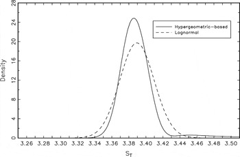
Lognormal and hypergeometric-based risk-neutral densities, 17 May 1996, 1 month maturity.
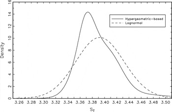
Lognormal and hypergeometric-based risk-neutral densities, 17 May 1996, 3-months to maturity.
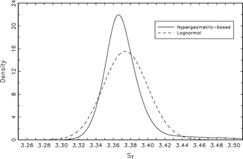
Lognormal and hypergeometric-based risk-neutral densities, 28 April 1997, 1 month maturity.
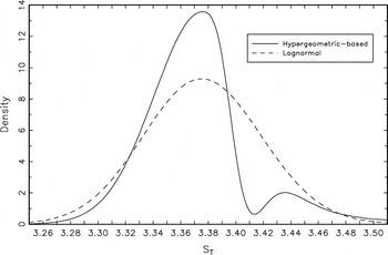
Lognormal and hypergeometric-based risk-neutral densities, 28 April 1997, 3-months to maturity.
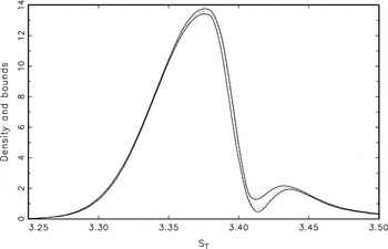
Sensitivity bounds for the hypergeometric-based density with one strike deleted at a time.
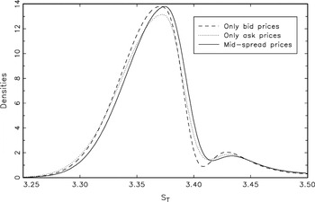
Hypergeometric-based estimated densities with ask, with bid, and with mid-spread option prices.
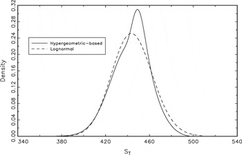
Lognormal and hypergeometric-based risk-neutral densities, S&P500 index options, 3 May 1993, 46-days to maturity.
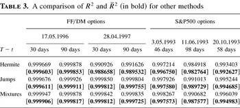
A comparison of R2 and R2 (in bold) for other methods
 You have
Access
- 26
- Cited by