


1. Introduction
A sticky reflecting jump diffusion process can be constructed as a time-changed version of the reflecting jump diffusion process. More precisely, first consider on  $[0,+\infty)$ the reflecting process
 $X=\{X_{t},t\geq 0\}$, which evolves according to the stochastic differential equation (SDE)
 \begin{align} {\mathrm{d}} X_{t}=\mu(X_{t}){\mathrm{d}} t+\sigma(X_{t}) {\mathrm{d}} W_{t}+{\mathrm{d}} V_{t}+{\mathrm{d}} L_{t}, \qquad X_{0}\geq 0,\end{align}
where  $W=\{W_{t},t\geq 0\}$ is a standard Brownian motion and
 $V=\{V_{t},t\geq 0\}$ is a compound Poisson process independent of W. The process
 $L=\{L_{t},t\geq 0\}$ with
 $L_{0}=0$ is usually called the regulator of X (see, e.g., [Reference Harrison10] and [Reference Asmussen and Pihlsgård1]), representing the magnitude of the displacement which is the minimal amount required to keep X nonnegative. The sample paths of L are nondecreasing, right continuous with left limits (RCLL), and satisfy
 \begin{align*}L_{t}=\int_{0}^{t}\textbf{1}_{\{X_{s}=0\}}{\mathrm{d}} L_{s},\qquad t>0.\end{align*}
Let us denote by  $L^{\rm c}=\{L^{\rm c}_{t}, t\geq 0\}$ the continuous part of L, i.e.
 $L^{\rm c}_{t}=L_{t}-\sum_{0<s\leq t}\Delta L_{s}$ where
 $\Delta L_{s}= L_{s}- L_{s-}$. Now, for an arbitrary given constant
 $\beta>0$, define the random time
 \begin{align*}\eta_{t}=t+\beta L^{\rm c}_{t}.\end{align*}
It is easy to see that the inverse  $\eta^{-1}_{t}=\inf\{s\geq0, \eta_{s}\geq t \}$ is continuous, strictly increasing, and satisfies
 \begin{align}\eta^{-1}_{t}=t-\beta L^{\rm c}_{\eta^{-1}_{t}},\end{align}
with  $\eta^{-1}_{0}=0$. Then a new process
 $Y=\{Y_{t},t\geq 0\}$ can be introduced by time-changing X based on
 $\eta^{-1}_{t}$:
 \begin{align}Y_{t}=X_{\eta^{-1}_{t}}.\end{align}
We call this process the sticky reflecting jump diffusion process, since under some restrictive conditions, the set of times that Y spends at the boundary 0 has positive Lebesgue measure, compared with zero Lebesgue measure for the reflecting case (1). What’s more, the above construction extends the one put forward by [Reference Yamada24] where only positive jumps are allowed in the jump part of the process and thus the regulator therein is continuous in time.
The process Y defined by (3) belongs to the class of sticky reflecting Markov processes which has found a variety of applications in finance, contract theory, storage, and queuing networks; see [Reference Harrison and Lemoine11, Reference Nie and Linetsky17, Reference Nie and Linetsky18, Reference Welch23–Reference Zhu25]. Those applications rely heavily on the detailed analysis of probabilistic properties of involved processes among which the distribution of the first passage time may be a rather important one. The aim of the current work is to investigate the first passage time of Y defined by
 \begin{align}\tau_{b}=\inf \{t\geq 0, Y_{t}\geq b\}\end{align}
when V in (1) is specified as a compound Poisson process with double exponential jumps; that is to say,  $V_{t}=\sum_{i=1}^{N_{t}}H_{i}$, where
 $N=\{N_{t},t\geq 0\}$ is a Poisson process with rate
 $\lambda$ and
 $\{H_{i}\}$ is a sequence of independent and identically distributed random variables with double exponential density
 \begin{align*}g_{H}(x)=\left\{\begin{array}{ll} \displaystyle p \delta_{1} {\rm e}^{-\delta_{1} x}, & x\geq 0, \\[5pt] \displaystyle q \delta_{2} {\rm e}^{\delta_{2} x}, & x
< 0. \end{array} \right.\end{align*}
The constants  $p,q\geq 0$,
 $p+q=1$, and
 $\delta_{1},\delta_{2}>0$. We also denote by
 $G({\mathrm{d}} x)$ the corresponding probability distribution of
 $H_{i}$ such that
 $G({\mathrm{d}} x)=g_{H}(x){\mathrm{d}} x$.
In the literature, the results on first passage problems for processes with one-sided jumps are quite abundant (see, e.g., [Reference Avram, Kyprianou and Pistorius3, Reference Bo, Ren, Wang and Yang5, Reference Doney7–Reference Hadjiev9, Reference Kella and Stadje13, Reference Novikov19, Reference Patie20]), while those for processes with two-sided jumps are relatively limited. Kou and Wang [Reference Kou and Wang15] studied the first passage time of the double exponential jump diffusion process (more specifically, the diffusion part is driven by a drifted Brownian motion), and Cai [Reference Cai6] considered the more general case with hyper-exponential jumps. Using the method of contour integrals, Jacobsen and Jensen [Reference Jacobsen and Jensen12] derived the joint Laplace transform of the first passage time and the matching undershoot of the piecewise deterministic Markov process with two-sided jumps by solving the related differential equations. Based on the same method, the explicit solutions to the first passage problem for the reflecting Ornstein–Uhlenbeck (OU) process with two-sided jumps were obtained by Bo [Reference Bo4]. Despite all these works, however, to date there are no published results regarding the first passage times of sticky reflecting jump diffusions. In fact, as far as we know, only one paper, by Yamada [Reference Yamada24], which is irrelevant to first passage problems and mainly focused on approximating storage models by reflecting or sticky Markov processes, has ever taken into account the jump case for sticky reflecting processes.
In this paper we study the first passage times of sticky reflecting diffusion processes with double exponential jumps. We start by presenting some fundamental properties of the process Y with double exponential jumps, including, for example, the semimartingale representation for Y and the relationship between the continuous part of  $\{L_{\eta^{-1}_{t}},t\geq 0\}$ and the local time of Y at 0. Then we provide the results associated with the joint Laplace transform of the first passage time and the corresponding overshoot of Y with general drift and diffusion coefficients. Finally, two solvable examples are considered, in which the diffusion part is driven by a drifted Brownian motion and by an OU process, respectively. Actually, using the same logic one can further get the analytical solutions for more general cases when jumps are hyper-exponential.
The rest of the paper is organized as follows. Section 2 exhibits some basic properties associated with Y. The general results on the first passage time of Y together with two concrete examples are provided in Section 3.
2. Preliminaries
2.1. Assumptions and some properties of Y
To begin with, we make two assumptions concerning the diffusion coefficient  $\sigma({\cdot})$ and the solutions of the SDE (1).
Assumption 2.1.  $\sigma({\cdot})$ is bounded below by a positive number.
Assumption 2.2. The SDE (1) with reflection on zero has a unique solution in the law sense.
Assumption 2.2 holds, for example, when the coefficients  $\mu({\cdot})$ and
 $\sigma({\cdot})$ are Lipschitz continuous and
 $\sigma({\cdot})$ is bounded. In fact, there exists a unique strong solution in such a case; see [Reference Atar and Budhiraja2].
Now let  $\skew2\widetilde{L}=\{\skew2\widetilde{L}_{t}=L_{\eta^{-1}_{t}},t\geq 0\}$ be the time-changed version of the regulator L, and
 $\skew2\widetilde{L}^{\rm c}=\{\skew2\widetilde{L}^{\rm c}_{t},t\geq 0\}$ the continuous part of
 $\skew2\widetilde{L}$. As will be seen, among others, the process Y admits a semimartingale representation and
 $\skew2\widetilde{L}^{\rm c}$ can be expressed in terms of Lebesgue integrals.
(i)
 $\eta^{-1}_{t}=\int_{0}^{t}\textbf{1}_{\{Y_{s}>0\}}{\mathrm{d}} s$.
(ii) On an extended probability space, there exist a standard Brownian motion
$\widetilde{W}=\{\widetilde{W}_{t},\break t\geq 0\}$ and a Poisson random measure $\skew2\widetilde{N}({\mathrm{d}} t, {\mathrm{d}} x)$ whose compensator is given by $\lambda G({\mathrm{d}} x){\mathrm{d}} t $, such that
(5)where\begin{align} Y_{t}=Y_{0}+\int_{0}^{t}\mu(Y_{s})\textbf{1}_{\{Y_{s}>0\}}{\mathrm{d}} s+\int_{0}^{t}\sigma(Y_{s})\textbf{1}_{\{Y_{s}>0\}}{\mathrm{d}} \widetilde{W}_{s}+\skew2\widetilde{V}_{t}+\skew2\widetilde{L}_{t}, \end{align}$\skew2\widetilde{V}_{t}=\int_{0}^{t}\int_{\mathbb{R}}x\textbf{1}_{\{Y_{s-}>0\}}\skew2\widetilde{N}({\mathrm{d}} s, {\mathrm{d}} x)$.(iii) The sample paths of
$\skew2\widetilde{L}$ are nondecreasing, RCLL, and satisfy
and\begin{align*} \skew2\widetilde{L}_{t}=\int_{0}^{t}\textbf{1}_{\{Y_{s}=0\}}{\mathrm{d}} \skew2\widetilde{L}_{s},\qquad t>0, \end{align*}\begin{align*} \Delta \skew2\widetilde{L}_{t}=(Y_{t-}+\Delta \skew2\widetilde{V}_{t})^{-}\triangleq \max(-(Y_{t-}+\Delta \skew2\widetilde{V}_{t}),0). \end{align*}(iv)
$\skew2\widetilde{L}^{\rm c}_{t}$ is absolutely continuous with respect to the Lebesgue measure:
\begin{align*} \skew2\widetilde{L}^{\rm c}_{t}=\frac{1}{\beta}\int_{0}^{t}\textbf{1}_{\{Y_{s}= 0\}}{\mathrm{d}} s. \end{align*}






Proof. The proof of (i) is similar to that of Theorem 3.1 in[Reference Salins and Spiliopoulos22] for sticky diffusion processes (without jumps). Since X is a semimartingale, it has a local time process  $l(a)=\{l_{t}(a),t\geq 0\}$ at each
 $a\in[0,+\infty)$ (see [Reference Protter21, p. 212]), and denote by
 $[X,X]^{\rm c}=\{[X,X]_{t}^{\rm c},t\geq 0\}$ the continuous part of the quadratic variation process of X. A direct application of the occupation time formula (see [Reference Protter21, p. 216, Corollary 1]) yields
 \begin{align*} \int_{0}^{t}\textbf{1}_{\{X_{s}=0\}}{\mathrm{d}} s=\int_{0}^{t}\frac{1}{\sigma^{2}(X_{s})}\textbf{1}_{\{X_{s}=0\}}{\mathrm{d}} [X,X]^{\rm c}_{s}=\int_{\{0\}}\frac{l_{t}(a)}{\sigma^{2}(a)}{\mathrm{d}} a=0, \end{align*}
which in turn implies that
 \begin{align} \int_{0}^{\eta^{-1}_{t}}\textbf{1}_{\{X_{s}=0\}}{\mathrm{d}} s&=\int_{0}^{t}\textbf{1}_{\{Y_{s}=0\}}{\mathrm{d}} \eta^{-1}_{s}\nonumber\\ &=\int_{0}^{t}\textbf{1}_{\{Y_{s}=0\}}{\mathrm{d}} s-\beta\int_{0}^{\eta^{-1}_{t}}\textbf{1}_{\{X_{s}=0\}}{\mathrm{d}} L_{s}^{\rm c}\nonumber\\ &=\int_{0}^{t}\textbf{1}_{\{Y_{s}=0\}}{\mathrm{d}} s-\beta L_{\eta^{-1}_{t}}^{\rm c}\nonumber\\ &=0 \end{align}
by virtue of the relation (2). From this fact, and using (2) again, we arrive at (i).
For assertion (ii), let  $N({\mathrm{d}} t,{\mathrm{d}} x)$ be the Poisson random measure associated with the compound Poisson process V, and
 $N^{*}({\mathrm{d}} t,{\mathrm{d}} x)=N({\mathrm{d}} t,{\mathrm{d}} x)-\lambda G({\mathrm{d}} x){\mathrm{d}} t$ the corresponding martingale measure. Then the SDE (1) can be rewritten as
 \begin{align*} {\mathrm{d}} X_{t}=\left[\mu(X_{t})+\lambda\left(\frac{p}{\delta_{1}}-\frac{q}{\delta_{2}}\right) \right]{\mathrm{d}} t+\sigma(X_{t}) {\mathrm{d}} W_{t}+\int_{\mathbb{R}}x N^{*}({\mathrm{d}} t,{\mathrm{d}} x)+{\mathrm{d}} L_{t}.\end{align*}
Now set  $U_{t}=\int_{0}^{t}\sigma(X_{s}) {\mathrm{d}} W_{s}+\int_{0}^{t}\int_{\mathbb{R}}x N^{*}({\mathrm{d}} s,{\mathrm{d}} x)$ and
 $\skew2\widetilde{U}_{t}=U_{\eta^{-1}_{t}}$. Following the idea of [Reference Yamada24, pp. 161–162], one can show, by virtue of the martingale argument and the optional sampling theorem, that on an extended probability space,
 \begin{align*} \skew2\widetilde{U}_{t}=\int_{0}^{t}\sigma(Y_{s})\textbf{1}_{\{Y_{s}>0\}} {\mathrm{d}} \widetilde{W}_{s}+\int_{0}^{t}\int_{\mathbb{R}}x \textbf{1}_{\{Y_{s}>0\}}\skew2\widetilde{N}^{*}({\mathrm{d}} s,{\mathrm{d}} x),\end{align*}
where  $\skew2\widetilde{N}^{*}({\mathrm{d}} t,{\mathrm{d}} x)=\skew2\widetilde{N}({\mathrm{d}} t,{\mathrm{d}} x)-\lambda G({\mathrm{d}} x){\mathrm{d}} t$. Thus it follows that
 \begin{align*} Y_{t}&=Y_{0}+\int_{0}^{t}\left[\mu(X_{\eta^{-1}_{s}})+\lambda\left(\frac{p}{\delta_{1}}-\frac{q}{\delta_{2}}\right) \right]{\mathrm{d}} \eta^{-1}_{s}+\skew2\widetilde{U}_{t}+\skew2\widetilde{L}_{t},\\ &=Y_{0}+\int_{0}^{t}\left[\mu(Y_{s})+\lambda\left(\frac{p}{\delta_{1}}-\frac{q}{\delta_{2}}\right) \right]\textbf{1}_{\{Y_{s}>0\}}{\mathrm{d}} s+\int_{0}^{t}\sigma(Y_{s})\textbf{1}_{\{Y_{s}>0\}} {\mathrm{d}} \widetilde{W}_{s}+\skew2\widetilde{V}_{t}\\ &\quad -\lambda\int_{0}^{t}\int_{\mathbb{R}}x \textbf{1}_{\{Y_{s}>0\}}G({\mathrm{d}} x){\mathrm{d}} s+\skew2\widetilde{L}_{t},\end{align*}
where for the second equality we use the property (i). This gives the expression (5).
To justify (iii), note that
 \begin{align*} \int_{0}^{t}\textbf{1}_{\{Y_{s}=0\}}{\mathrm{d}} \skew2\widetilde{L}_{s}= \int_{0}^{\eta^{-1}_{t}}\textbf{1}_{\{X_{s}=0\}}{\mathrm{d}} L_{s}=L_{\eta^{-1}_{t}}=\skew2\widetilde{L}_{t}.\end{align*}
Also, the representation (see [Reference Asmussen and Pihlsgård1] or [Reference Bo4])
 \begin{align}\Delta L_{t}=(X_{t-}+\Delta V_{t})^{-}\end{align}
suggests that
 \begin{align*} \Delta \skew2\widetilde{L}_{t} & = L_{\eta^{-1}_{t}}-L_{\eta^{-1}_{t}-}=(X_{\eta^{-1}_{t}-}+U_{\eta^{-1}_{t}}-U_{\eta^{-1}_{t}-})^{-} \\ & = (Y_{t-}+\Delta \skew2\widetilde{U}_{t})^{-}=(Y_{t-}+\Delta \skew2\widetilde{V}_{t})^{-}.\end{align*}
The last assertion comes from (6) and the fact that
 \begin{align} L^{\rm c}_{\eta^{-1}_{t}} & = L_{\eta^{-1}_{t}}-\sum_{0<s\leq \eta^{-1}_{t}}\Delta L_{s}=L_{\eta^{-1}_{t}}-\sum_{0<s\leq t}\left(L_{\eta^{-1}_{s}}-L_{\eta^{-1}_{s}-}\right) \nonumber \\ & = \skew2\widetilde{L}_{t}-\sum_{0<s\leq t}\Delta \skew2\widetilde{L}_{s} =\skew2\widetilde{L}^{\rm c}_{t}.\end{align}
This completes the proof.
The construction (3) together with the above proposition guarantee the existence of solutions of the SDE (5). Moreover, repeating the argument in the proof of Proposition 1 in [Reference Yamada24] with only minor changes, we obtain the following uniqueness result.
Remark 2.1. Based on this proposition and by the same argument as in Remark 6.1 in [Reference Yamada24], we conclude that if Y starts at 0, then 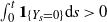 $\int_{0}^{t}\textbf{1}_{\{Y_{s}= 0\}}{\mathrm{d}} s>0$ for all
 $t>0$. In contrast,
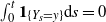 $\int_{0}^{t}\textbf{1}_{\{Y_{s}= y\}}{\mathrm{d}} s=0$ for any
 $y>0$. Therefore, 0 is a sticky reflecting boundary of Y.
2.2. The relationship between $\skew2\widetilde{L}^{\rm c}$ and the local time of Y at 0

The semimartingale representation (5) enables us to define the local time of Y at the boundary 0, denoted by  $\skew2\widetilde{l}(0)=\{\skew2\widetilde{l}_{t}(0),t\geq 0\}$, in the sense of [Reference Protter21, p. 212]. It is a nondecreasing continuous process which increases only at the time set
 $\{t>0, Y_{t}=0\}$ (see [Reference Protter21, p. 214, Theorem 69]). The same properties hold for
 $\skew2\widetilde{L}^{\rm c}$ as implied by Proposition 2.1. What is presented below clarifies the relationship between these two processes.
 \begin{align}\skew2\widetilde{L}^{\rm c}_{t}=\frac{1}{2}\skew2\widetilde{l}_{t}(0), \qquad t\geq 0.\end{align}
Proof. We proceed by first proving  ${L}^{\rm c}_{t}=\frac{1}{2}{l}_{t}(0)$ (recalling that l(0) denotes the local time of the process X at 0). Using (1) and the Meyer–Itô formula (see [Reference Protter21, p. 214, Theorem 70]), we have
 \begin{align}X_{t}^{+}&=X_{0}^{+}+\int_{0}^{t}\textbf{1}_{\{X_{s-}>0\}}{\mathrm{d}} X_{s}+\sum_{0<s\leq t}\left(X^{+}_{s}-X^{+}_{s-}-\textbf{1}_{\{X_{s-}>0\}}\Delta X_{s}\right)+\frac{1}{2}{l}_{t}(0)\nonumber\\ &=X_{0}+\int_{0}^{t}\mu(X_{s})\textbf{1}_{\{X_{s}>0\}}{\mathrm{d}} {s}+\int_{0}^{t}\sigma(X_{s})\textbf{1}_{\{X_{s}>0\}}{\mathrm{d}} W_{s}+\int_{0}^{t}\textbf{1}_{\{X_{s}>0\}}{\mathrm{d}} L^{\rm c}_{s}\nonumber\\ &\quad+\sum_{0<s\leq t}\Delta X_{s}+\frac{1}{2}{l}_{t}(0).\end{align}
Observe that
 \begin{align*}\Delta X_{t}=\Delta V_{t}+(X_{t-}+\Delta V_{t})^{-}=\left\{\begin{array}{l@{\quad}l} \displaystyle -X_{t-}, &X_{t-}+\Delta V_{t}
< 0,\\[5pt] \displaystyle \Delta V_{t}, & X_{t-}+\Delta V_{t}\geq 0. \end{array} \right.\end{align*}
Then the series term appearing in (10) can be expressed in integral form:
 \begin{align*}\sum_{0<s\leq t}\Delta X_{s}=\int_{0}^{t}\int_{\mathbb{R}}\left[x-(X_{s-}+x) \textbf{1}_{\{X_{s-}+x<0\}}\right]{N}({\mathrm{d}} s,{\mathrm{d}} x).\end{align*}
On the other hand, the SDE (1) implies that
 \begin{align}X^{+}_{t} & = X_{0}+\int_{0}^{t}\mu(X_{s}){\mathrm{d}} s+\int_{0}^{t}\sigma(X_{s}){\mathrm{d}} W_{s} \nonumber \\ & \quad + \int_{0}^{t}\int_{\mathbb{R}}\left[x-(X_{s-}+x) \textbf{1}_{\{X_{s-}+x<0\}}\right]{N}({\mathrm{d}} s,{\mathrm{d}} x)+L^{\rm c}_{t},\end{align}
because  $X_{t}\geq 0$ and
 \begin{align*}L_{t}=L^{\rm c}_{t}+\sum_{0<s\leq t}\Delta L_{s}=L^{\rm c}_{t}-\int_{0}^{t}\int_{\mathbb{R}}(X_{s-}+x) \textbf{1}_{\{X_{s-}+x<0\}}{N}({\mathrm{d}} s,{\mathrm{d}} x)\end{align*}
by (7). As a consequence, the combination of (10) and (11) produces
 \begin{align*}L^{\rm c}_{t}=-\int_{0}^{t}\mu(X_{s})\textbf{1}_{\{X_{s}=0\}}{\mathrm{d}} {s}-\int_{0}^{t}\sigma(X_{s})\textbf{1}_{\{X_{s}=0\}}{\mathrm{d}} W_{s}+\frac{1}{2}{l}_{t}(0).\end{align*}
Since 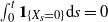 $\int_{0}^{t}\textbf{1}_{\{X_{s}=0\}}{\mathrm{d}} s=0$, the first and second terms on the right-hand side of the above equality vanish. This leads to the result
 ${L}^{\rm c}_{t}=\frac{1}{2}{l}_{t}(0)$.
To prove (9), noting that  $\skew2\widetilde{L}^{\rm c}_{t}=L^{\rm c}_{\eta^{-1}_{t}}=\frac{1}{2}{l}_{\eta^{-1}_{t}}(0)$ (see (8)), it suffices to show that
 ${l}_{\eta^{-1}_{t}}(0)=\skew2\widetilde{l}_{t}(0)$. According to the definition of the local time,
 ${l}_{\eta^{-1}_{t}}(0)$ and
 $\skew2\widetilde{l}_{t}(0)$ are the continuous parts of
 \begin{align}|X_{\eta^{-1}_{t}}|-|X_{0}|-\int_{0}^{\eta^{-1}_{t}}{\rm sign}(X_{s-}){\mathrm{d}} X_{s}\end{align}
and
 \begin{align}|Y_{t}|-|Y_{0}|-\int_{0}^{t}{\rm sign}(Y_{s-}){\mathrm{d}} Y_{s},\end{align}
respectively, where  ${\rm sign}(x)$ represents the sign function that is equal to 1 if
 $x>0$ and equal to -1 otherwise. But, from Theorem 3.1 in[Reference Kobayashi14] we know that (12) and (13) are equal, which completes the proof.
3. First passage times
In this section we study the joint Laplace transform of the first passage time defined by (4) and the corresponding overshoot of Y:
 \begin{align}\mathrm{E}_{y}[{\rm e}^{-\theta \tau_{b}-\zeta (Y_{\tau_{b}}-b)}], \qquad 0\leq y\leq b.\end{align}
As the first step, we consider the case of general drift and diffusion coefficients. Then we try to work out the explicit solutions for two special cases when the diffusion part is driven by a drifted Brownian motion and by an OU process.
3.1. General results
Let us introduce an integro-differential operator  $\mathcal{A}$ defined as follows:
 \begin{align*} \mathcal{A}\,f(x)&=\frac{1}{2}\sigma^{2}(x)\,f''(x)+\mu(x) f'(x) \\ &\quad+\lambda\left[\,f(0)G((\!-\infty,-x))-f(x)+\int_{-x}^{+\infty}f(x+u)G({\mathrm{d}} u)\right]. \end{align*}
The theorem below states that, for a function satisfying an integro-differential equation associated with  $\mathcal{A}$ and certain restrictive conditions (including a boundary condition at 0), it admits a stochastic representation concerning the first passage time of Y.
Theorem 3.1. Let  $\theta>0$ and
 $\zeta\geq 0$. Assume that
 $f({\cdot})$ is a bounded function defined on
 $[0,+\infty)$ which is of class
 $\mathcal {C}^{2}$ on [0, b] and takes the form
 \begin{align*}f(x)=C{\rm e}^{-\zeta (x-b)}\end{align*}
on  $(b,+\infty)$, where C is a constant. Moreover, on [0, b] it satisfies
 \begin{numcases}
\!\!\!\!\displaystyle \mathcal {A}f(x)=\theta f(x),\gdef\@equationnumber{(15)}\\
\!\!\displaystyle f'(0)=\beta\theta f(0).\gdef\@equationnumber{(16)}
\end{numcases}
 \begin{equation}\begin{cases} \displaystyle f'(0)=\beta\theta f(0).\end{cases}\end{equation}
Then it holds that, for  $0\leq y\leq b$,
 \begin{align}f(y)=f(b)\mathrm{E}_{y}\,\left[{\rm e}^{-\theta \tau_{b}}\textbf{1}_{\{\tau_{b}<+\infty,Y_{\tau_{b}}=b\}}\right]+C\mathrm{E}_{y}\,\left[{\rm e}^{-\theta \tau_{b}-\zeta (Y_{\tau_{b}}-b)}\textbf{1}_{\{\tau_{b}<+\infty,Y_{\tau_{b}}>b\}}\right].\end{align}
Proof. Recall the notation in the proof of Proposition 2.1. By Itô’s formula (see [Reference Protter21, p. 78, Theorem 32]) and the semimartingale representation (5) for Y, we have
 \begin{align}&{\rm e}^{-\theta (\tau_{b}\wedge t)}f(Y_{\tau_{b}\wedge t})\nonumber\\&\quad=f(Y_{0})+\int_{0}^{\tau_{b}\wedge t}{\rm e}^{-\theta s}\left[\frac{1}{2}\sigma^{2}(Y_{s})\,f''(Y_{s})\textbf{1}_{\{Y_{s}>0\}}+\mu(Y_{s})\,f'(Y_{s})\textbf{1}_{\{Y_{s}>0\}}-\theta f(Y_{s})\right]{\mathrm{d}} s\nonumber\\&\quad\quad+\int_{0}^{\tau_{b}\wedge t}{\rm e}^{-\theta s}\sigma(Y_{s})\,f'(Y_{s})\textbf{1}_{\{Y_{s}>0\}}{\mathrm{d}} \widetilde{W}_{s}+f'(0)\int_{0}^{\tau_{b}\wedge t}{\rm e}^{-\theta s}{\mathrm{d}} \skew2\widetilde{L}^{\rm c}_{s}\nonumber\\&\quad\quad+\int_{0}^{\tau_{b}\wedge t}\int_{\mathbb{R}}{\rm e}^{-\theta s}\textbf{1}_{\{Y_{s-}>0\}}[\,f(0)\textbf{1}_{\{Y_{s-}+x<0\}} \nonumber \\& \quad\quad\qquad\qquad\qquad\qquad\qquad\qquad +\ f(Y_{s-}+x)\textbf{1}_{\{Y_{s-}+x\geq 0\}}-f(Y_{s-})]\skew2\widetilde{N}^{*}({\mathrm{d}} s,{\mathrm{d}} x)\nonumber\\&\quad\quad+\lambda\int_{0}^{\tau_{b}\wedge t}\int_{\mathbb{R}}{\rm e}^{-\theta s}\textbf{1}_{\{Y_{s-}>0\}}[\,f(0)\textbf{1}_{\{Y_{s-}+x<0\}} \nonumber \\& \quad\quad\qquad\qquad\qquad\qquad\qquad\qquad +\ f(Y_{s-}+x)\textbf{1}_{\{Y_{s-}+x\geq 0\}}-f(Y_{s-})]\,G({\mathrm{d}} x){\mathrm{d}} s,\end{align}
where we use the relation (which is evident from (iv) in Proposition 2.1)
 \begin{align*}\skew2\widetilde{L}^{\rm c}_{t}=\int_{0}^{t}\textbf{1}_{\{Y_{s}=0\}}{\mathrm{d}} \skew2\widetilde{L}^{\rm c}_{s},\end{align*}
the equality
 \begin{multline*}f(0)\textbf{1}_{\{Y_{s-}+x\textbf{1}_{\{Y_{s-}>0\}}<0\}}+f\left(Y_{s-}+x\textbf{1}_{\{Y_{s-}>0\}}\right)\textbf{1}_{\{Y_{s-}+x\textbf{1}_{\{Y_{s-}>0\}}\geq 0\}}-f(Y_{s-})\\=\textbf{1}_{\{Y_{s-}>0\}}[\,f(0)\textbf{1}_{\{Y_{s-}+x<0\}}+f(Y_{s-}+x)\textbf{1}_{\{Y_{s-}+x\geq 0\}}-f(Y_{s-})]\end{multline*}
for  $0\leq s\leq \tau_{b}\wedge t$, and the fact that
 \begin{align*}\Delta Y_{t}=\Delta \skew2\widetilde{V}_{t}+\Delta\skew2\widetilde{L}_{t}=\left\{\begin{array}{ll} \displaystyle -Y_{t-}, &Y_{t-}+\Delta \skew2\widetilde{V}_{t}
< 0,\\[5pt] \displaystyle \Delta \skew2\widetilde{V}_{t}, & Y_{t-}+\Delta \skew2\widetilde{V}_{t}\geq 0. \end{array} \right.\end{align*}
Thanks to the property (iv) in Proposition 2.1, the second term on the right-hand side can be rewritten as
 \begin{align*}&\int_{0}^{\tau_{b}\wedge t}{\rm e}^{-\theta s}\left[\frac{1}{2}\sigma^{2}(Y_{s})\,f''(Y_{s})+\mu(Y_{s})\,f'(Y_{s})-\theta f(Y_{s})\right]{\mathrm{d}} s\\&\quad\quad-\beta\left(\frac{1}{2}\sigma^{2}(0)\,f''(0)+\mu(0)\,f'(0)\right)\int_{0}^{\tau_{b}\wedge t}{\rm e}^{-\theta s}{\mathrm{d}} \skew2\widetilde{L}^{\rm c}_{s},\end{align*}
and the last term is equal to
 \begin{multline*}\lambda\int_{0}^{\tau_{b}\wedge t}\int_{\mathbb{R}}{\rm e}^{-\theta s}[\,f(0)\textbf{1}_{\{Y_{s-}+x \lt 0\}}+f(Y_{s-}+x)\textbf{1}_{\{Y_{s-}+x\geq 0\}}-f(Y_{s-})]G({\mathrm{d}} x){\mathrm{d}} s\\-\beta\lambda\left[\,f(0)G((\!-\infty,0))-f(0)+\int_{0}^{+\infty}f(x)G({\mathrm{d}} x)\right]\int_{0}^{\tau_{b}\wedge t}{\rm e}^{-\theta s}{\mathrm{d}} \skew2\widetilde{L}^{\rm c}_{s}.\end{multline*}
Substituting these into (18) gives
 \begin{align*}&{\rm e}^{-\theta (\tau_{b}\wedge t)}f(Y_{\tau_{b}\wedge t})\\&\quad=f(Y_{0})+\int_{0}^{\tau_{b}\wedge t}{\rm e}^{-\theta s}\left[\mathcal{A}\,f(Y_{s})-\theta f(Y_{s})\right]{\mathrm{d}} s+\int_{0}^{\tau_{b}\wedge t}{\rm e}^{-\theta s}\sigma(Y_{s})\,f'(Y_{s})\textbf{1}_{\{Y_{s}>0\}}{\mathrm{d}} \widetilde{W}_{s}\\&\quad\quad+\int_{0}^{\tau_{b}\wedge t}\int_{\mathbb{R}}{\rm e}^{-\theta s}\textbf{1}_{\{Y_{s-}>0\}}[\,f(0)\textbf{1}_{\{Y_{s-}+x \lt 0\}} \\&\quad\quad\qquad\qquad\qquad\qquad\qquad\qquad\left. +\ f(Y_{s-}+x)\textbf{1}_{\{Y_{s-}+x\geq 0\}}-f(Y_{s-})\right]\skew2\widetilde{N}^{*}({\mathrm{d}} s,{\mathrm{d}} x)\\&\quad\quad+[\,f'(0)-\beta \mathcal{A}\,f(0) ]\int_{0}^{\tau_{b}\wedge t}{\rm e}^{-\theta s}{\mathrm{d}} \skew2\widetilde{L}^{\rm c}_{s}.\end{align*}
It then follows from (15) and (16) that, conditional on  $Y_{0}=y\in[0,b]$,
 \begin{align*}f(y)&=\mathrm{E}_{y}[{\rm e}^{-\theta (\tau_{b}\wedge t)}f(Y_{\tau_{b}\wedge t})]\\ &=\mathrm{E}_{y}[{\rm e}^{-\theta (\tau_{b}\wedge t)}f(Y_{\tau_{b}\wedge t})\textbf{1}_{\{\tau_{b}<+\infty\}}]+\mathrm{E}_{y}\left[{\rm e}^{-\theta t}f\left(Y_{ t}\right)\textbf{1}_{\{\tau_{b}=+\infty\}}\right]\!.\end{align*}
Finally, letting  $t\rightarrow +\infty$, we arrive at the desired result using the dominated convergence theorem and the boundedness of
 $f({\cdot})$.
The next corollary is immediate from the above theorem.
Corollary 3.1. Assume that  $f_{i}({\cdot})$,
 $i=1,2$, are two linearly independent
 $\mathcal {C}^{2}$ functions defined on [0, b]. Define
 \begin{align*} \skew2\widetilde{f}_{1}(x)=\left\{\begin{array}{l@{\quad}l} \displaystyle f_{1}(x), & 0\leq x\leq b,\\[5pt] \displaystyle 0, & x>b, \end{array} \right.\qquad \skew2\widetilde{f}_{2}(x)=\left\{\begin{array}{l@{\quad}l} \displaystyle f_{2}(x), & 0\leq x\leq b,\\[5pt] \displaystyle e^{-\zeta (x-b)}, & x>b. \end{array} \right.\end{align*}
If both  $\skew2\widetilde{f}_{i}({\cdot})$,
 $i=1,2$, satisfy (15) and (16) on [0, b], then
 \begin{align}\mathrm{E}_{y}[{\rm e}^{-\theta \tau_{b}-\zeta (Y_{\tau_{b}}-b)}]=\frac{f_{1}(y)\left[1-f_{2}(b)\right]+f_{2}(y)\,f_{1}(b)}{f_{1}(b)},\qquad 0\leq y\leq b.\end{align}
Proof. Note that  $\skew2\widetilde{f}_{1}({\cdot})$ satisfies the assumptions of Theorem 3.1 when
 $C=0$. An application of Theorem 3.1 to
 $\skew2\widetilde{f}_{i}({\cdot})$,
 $i=1,2$, solving the resulting system of equations, and using the relation
 \begin{align*} \mathrm{E}_{y}[{\rm e}^{-\theta \tau_{b}-\zeta (Y_{\tau_{b}}-b)}]= \mathrm{E}_{y}[{\rm e}^{-\theta \tau_{b}}\textbf{1}_{\{\tau_{b}<+\infty,Y_{\tau_{b}}=b\}}]+\mathrm{E}_{y}[{\rm e}^{-\theta \tau_{b}-\zeta (Y_{\tau_{b}}-b)}\textbf{1}_{\{\tau_{b}<+\infty,Y_{\tau_{b}}>b\}}]\end{align*}
complete the derivation of (19).
Remark 3.1. It is impossible for the denominator  $f_{1}(b)$ in (19) to be equal to 0 since if so, one would deduce from (17) that
 $f_{1}({\cdot})\equiv 0$ on [0, b]. This contradicts the hypothesis that
 $f_{i}({\cdot})$,
 $i=1,2$, are linearly independent.
Consequently, to compute the joint Laplace transform (14) for a specific sticky reflecting process Y, we merely need to find two linearly independent functions  $f_{i}({\cdot})$,
 $i=1,2$, as in Corollary 3.1.
3.2. Example 1: sticky reflecting drifted Brownian motion with double exponential jumps
We assume that the coefficients in (1) are given by  $\mu(x)\equiv \mu$ and
 $\sigma(x)\equiv \sigma$, and the process Y is thus called the sticky reflecting drifted Brownian motion with double exponential jumps. A preliminary lemma [Reference Kou and Wang15, Lemma 2.1] will be offered before addressing the related first passage problem.
Lemma 3.1. The algebraic equation
 \begin{align*}\frac{\sigma^{2}}{2}x^{2}+\mu x+\lambda\left(\frac{p\delta_{1}}{\delta_{1}-x}+\frac{q\delta_{2}}{\delta_{2}+x}-1\right)=\theta,\end{align*}
with  $\theta>0$, has exactly four roots:
 $\varepsilon_{i}$,
 $i=1,2,3,4$, which meet
 \begin{align} -\infty<\varepsilon_{1}<-\delta_{2}<\varepsilon_{2}<0<\varepsilon_{3}<\delta_{1}<\varepsilon_{4}<+\infty.\end{align}
Then we have
Proposition 3.1. The two linearly independent functions  $f_{i}({\cdot})$,
 $i=1,2$, introduced in Corollary 3.1 can be chosen as
 \begin{align*} f_{1}(x)=\sum_{i=1}^{3}C_{i}^{(1)}{\rm e}^{\varepsilon_{i}(x-b)}+{\rm e}^{\varepsilon_{4}(x-b)},\qquad f_{2}(x)=\sum_{i=1}^{3}C_{i}^{(2)}{\rm e}^{\varepsilon_{i}(x-b)},\end{align*}
where 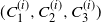 $(C_{1}^{(i)},C_{2}^{(i)},C_{3}^{(i)})$,
 $i=1,2$, are unique solutions of the equation systems
 \begin{align}\left\{\begin{array}{l} \displaystyle \sum_{i=1}^{3}\frac{\varepsilon_{i}C_{i}}{\varepsilon_{i}+\delta_{2}}{\rm e}^{-\varepsilon_{i}b}=-\frac{\varepsilon_{4}}{\varepsilon_{4}+\delta_{2}}{\rm e}^{-\varepsilon_{4}b},\\[5pt] \displaystyle \sum_{i=1}^{3}\frac{C_{i}}{\varepsilon_{i}-\delta_{1}}=-\frac{1}{\varepsilon_{4}-\delta_{1}}, \\[5pt] \displaystyle \sum_{i=1}^{3}C_{i}(\varepsilon_{i}-\beta \theta){\rm e}^{-\varepsilon_{i}b}=-(\varepsilon_{4}-\beta \theta){\rm e}^{-\varepsilon_{4}b}, \end{array} \right.\quad \left\{\begin{array}{l} \displaystyle \sum_{i=1}^{3}\frac{\varepsilon_{i}C_{i}}{\varepsilon_{i}+\delta_{2}}{\rm e}^{-\varepsilon_{i}b}=0,\\[5pt] \displaystyle \sum_{i=1}^{3}\frac{C_{i}}{\varepsilon_{i}-\delta_{1}}=-\frac{1}{\zeta+\delta_{1}}, \\[5pt] \displaystyle \sum_{i=1}^{3}C_{i}(\varepsilon_{i}-\beta \theta){\rm e}^{-\varepsilon_{i}b}=0, \end{array} \right.\end{align}
respectively.
Proof. Consider the function  $f({\cdot})$ of the form
 \begin{align*}f(x)=\left\{\begin{array}{ll} \displaystyle \sum_{i=1}^{4}C_{i}{\rm e}^{\varepsilon_{i}(x-b)},& 0\leq x\leq b,\\[5pt] \displaystyle C{\rm e}^{-\zeta (x-b)},& x>b. \end{array} \right.\end{align*}
By computation, we obtain that, for  $0\leq x\leq b$,
 \begin{align*}\mathcal{A}\,f(x)-\theta f(x)&=\lambda q {\rm e}^{-\delta_{2}x}\sum_{i=1}^{4}\frac{\varepsilon_{i}C_{i}}{\varepsilon_{i}+\delta_{2}}{\rm e}^{-\varepsilon_{i}b}+\lambda p \delta_{1}{\rm e}^{\delta_{1}(x-b)}\left(\sum_{i=1}^{4}\frac{C_{i}}{\varepsilon_{i}-\delta_{1}}+\frac{C}{\zeta+\delta_{1}}\right)\\&\quad+\sum_{i=1}^{4}C_{i}{\rm e}^{\varepsilon_{i}(x-b)}\left[\frac{\sigma^{2}\varepsilon_{i}^{2}}{2}+\mu \varepsilon_{i}+\lambda\left(\frac{p\delta_{1}}{\delta_{1}-\varepsilon_{i}}+\frac{q\delta_{2}}{\delta_{2}+\varepsilon_{i}}-1\right)-\theta\right]\!.\end{align*}
To employ Corollary 3.1, we impose the conditions (15) and (16) on  $f({\cdot})$ on [0, b]. Then, in light of Lemma 3.1, the system of equations
 \begin{equation}\begin{cases} \displaystyle \sum_{i=1}^{4}\frac{\varepsilon_{i}C_{i}}{\varepsilon_{i}+\delta_{2}}{\rm e}^{-\varepsilon_{i}b}=0,\nonumber\\ \displaystyle \sum_{i=1}^{4}\frac{C_{i}}{\varepsilon_{i}-\delta_{1}}+\frac{C}{\zeta+\delta_{1}}=0, \nonumber\\ \displaystyle \sum_{i=1}^{4}C_{i}(\varepsilon_{i}-\beta \theta){\rm e}^{-\varepsilon_{i}b}=0 \nonumber\end{cases}\end{equation}
must hold, where the last equation is a result of (16). If we denote by  $(C_{1},C_{2},C_{3},C_{4},C)$ the solution of the above equation system, we find that
 $(C_{1}^{(1)},C_{2}^{(1)},C_{3}^{(1)},1,0)$ and
 $(C_{1}^{(2)},C_{2}^{(2)},C_{3}^{(2)},0,1)$ are two linearly independent solutions, which correspond to two linearly independent functions
 $f_{1}({\cdot})$ and
 $f_{2}({\cdot})$, respectively. Now it remains to show that the coefficient matrix of the linear equation systems in (21) is nonsingular for any
 $\theta>0$. In fact, the determinant of the coefficient matrix
 \begin{align*}\Phi=\begin{bmatrix} \displaystyle \frac{\varepsilon_{1}}{\varepsilon_{1}+\delta_{2}}{\rm e}^{-\varepsilon_{1}b} & \displaystyle \frac{\varepsilon_{2}}{\varepsilon_{2}+\delta_{2}}{\rm e}^{-\varepsilon_{2}b} & \displaystyle \frac{\varepsilon_{3}}{\varepsilon_{3}+\delta_{2}}{\rm e}^{-\varepsilon_{3}b} \\ \\ \displaystyle \frac{1}{\varepsilon_{1}-\delta_{1}} & \displaystyle \frac{1}{\varepsilon_{2}-\delta_{1}} & \displaystyle \frac{1}{\varepsilon_{3}-\delta_{1}} \\ \\ \displaystyle (\varepsilon_{1}-\beta \theta){\rm e}^{-\varepsilon_{1}b} &\displaystyle (\varepsilon_{2}-\beta \theta){\rm e}^{-\varepsilon_{2}b} & \displaystyle (\varepsilon_{3}-\beta \theta){\rm e}^{-\varepsilon_{3}b}\end{bmatrix}\end{align*}
is given by
 \begin{align*}\det(\Phi)=\frac{(T_{1,\theta}\delta_{2}\beta\theta+T_{2,\theta})\prod_{1\leq i \leq 3}{\rm e}^{-b\varepsilon_{i}}}{\prod_{1\leq i, j\leq 3}(\delta_{1}-\varepsilon_{i})(\delta_{2}+\varepsilon_{j})},\end{align*}
where (recalling from Lemma 3.1 that the roots  $\{\varepsilon_{i}\}$ are actually dependent on
 $\theta$)
 \begin{align*}T_{1,\theta}&={\rm e}^{\varepsilon_{1}b}(\delta_{1}-\varepsilon_{2})(\delta_{1}-\varepsilon_{3})(\delta_{2}+\varepsilon_{1})(\varepsilon_{3}-\varepsilon_{2})+{\rm e}^{\varepsilon_{2}b}(\delta_{1}-\varepsilon_{1})(\delta_{1}-\varepsilon_{3})(\delta_{2}+\varepsilon_{2})(\varepsilon_{1}-\varepsilon_{3})\\ &\quad +{\rm e}^{\varepsilon_{3}b}(\delta_{1}-\varepsilon_{1})(\delta_{1}-\varepsilon_{2})(\delta_{2}+\varepsilon_{3})(\varepsilon_{2}-\varepsilon_{1}),\end{align*}
and
 \begin{align*}T_{2,\theta}&={\rm e}^{\varepsilon_{1}b}(\delta_{1}-\varepsilon_{2})(\delta_{1}-\varepsilon_{3})(\delta_{2}+\varepsilon_{1})(\varepsilon_{3}-\varepsilon_{2})\varepsilon_{2}\varepsilon_{3}\\&\quad +{\rm e}^{\varepsilon_{2}b}(\delta_{1}-\varepsilon_{1})(\delta_{1}-\varepsilon_{3})(\delta_{2}+\varepsilon_{2})(\varepsilon_{1}-\varepsilon_{3})\varepsilon_{1}\varepsilon_{3}\\&\quad +{\rm e}^{\varepsilon_{3}b}(\delta_{1}-\varepsilon_{1})(\delta_{1}-\varepsilon_{2})(\delta_{2}+\varepsilon_{3})(\varepsilon_{2}-\varepsilon_{1})\varepsilon_{1}\varepsilon_{2}.\end{align*}
The distribution of  $\{\varepsilon_{i}\}$ displayed in (20) implies that
 \begin{align*}T_{1,\theta}&> (\delta_{1}-\varepsilon_{2})(\delta_{1}-\varepsilon_{3})(\delta_{2}+\varepsilon_{1})(\varepsilon_{3}-\varepsilon_{2})+(\delta_{1}-\varepsilon_{1})(\delta_{1}-\varepsilon_{3})(\delta_{2}+\varepsilon_{2})(\varepsilon_{1}-\varepsilon_{3})\\ &\quad+(\delta_{1}-\varepsilon_{1})(\delta_{1}-\varepsilon_{2})(\delta_{2}+\varepsilon_{3})(\varepsilon_{2}-\varepsilon_{1})\\ &=(\delta_{1}+\delta_{2})(\varepsilon_{2}-\varepsilon_{1})(\varepsilon_{1}-\varepsilon_{3})(\varepsilon_{2}-\varepsilon_{3})\\ &\quad >0,\end{align*}
and that  $T_{2,\theta}>0$. Hence,
 $\det\!(\Phi) \lt 0$ for each
 $\theta>0$, which completes the proof.
When  $\lambda=0$, the process Y degenerates to the sticky reflecting drifted Brownian motion (without jumps). Since Y can only cross b by continuity in such a case, we have
 $Y_{\tau_{b}}=b$. Accordingly, the expression (17) in Theorem 3.1 becomes
 \begin{align}f(y)=f(b)\mathrm{E}_{y}[{\rm e}^{-\theta \tau_{b}}].\end{align}
Moreover, the two roots of the equation appearing in Lemma 3.1 with  $\lambda=0$ are given by
 \begin{align*}\widetilde{\varepsilon}_{1}=\frac{-\mu+\sqrt{\mu^{2}+2\theta \sigma^{2}}}{\sigma^{2}},\qquad \widetilde{\varepsilon}_{2}=\frac{-\mu-\sqrt{\mu^{2}+2\theta \sigma^{2}}}{\sigma^{2}}.\end{align*}
Proposition 3.2. When  $\lambda=0$,
 \begin{align*}\mathrm{E}_{y}\left[{\rm e}^{-\theta \tau_{b}}\right]=\frac{\left(\widetilde{\varepsilon}_{2}-\beta\theta\right){\rm e}^{\widetilde{\varepsilon}_{1}y-\widetilde{\varepsilon}_{2}b}-\left(\widetilde{\varepsilon}_{1}-\beta\theta\right){\rm e}^{\widetilde{\varepsilon}_{2}(y-b)}}{\left(\widetilde{\varepsilon}_{2}-\beta\theta\right){\rm e}^{\left(\widetilde{\varepsilon}_{1}-\widetilde{\varepsilon}_{2}\right)b}-\widetilde{\varepsilon}_{1}+\beta\theta}, \qquad 0\leq y\leq b.\end{align*}
Proof. For the function  $f({\cdot})$ of the form
 \begin{align*}f(x)=\left\{\begin{array}{l@{\quad}l} \displaystyle \sum_{i=1}^{2}C_{i}{\rm e}^{\widetilde{\varepsilon}_{i}(x-b)},& 0\leq x\leq b,\\[5pt] \displaystyle 0,& x>b, \end{array} \right.\end{align*}
it is straightforward to see that  $\mathcal{A}\,f(x)-\theta f(x)=0$,
 $0\leq x \leq b$. Hence, to utilize Theorem 3.1,
 $f({\cdot})$ needs to satisfy the condition (16), thereby suggesting that
 \begin{align*} \sum_{i=1}^{2}C_{i}(\widetilde{\varepsilon}_{i}-\beta \theta){\rm e}^{-\widetilde{\varepsilon}_{i}b}=0.\end{align*}
We may choose  $C_{2}=1$ and thus
 $C_{1}=-\frac{\widetilde{\varepsilon}_{2}-\beta \theta}{\widetilde{\varepsilon}_{1}-\beta \theta}{\rm e}^{\left(\widetilde{\varepsilon}_{1}-\widetilde{\varepsilon}_{2}\right)b}$. This leads to the desired result immediately with the help of (22).
3.3. Example 2: sticky reflecting OU process with double exponential jumps
We assume that the coefficients in (1) are given by  $\mu(x)=-\alpha x$ and
 $\sigma(x)\equiv \sigma$ with
 $\alpha, \sigma >0$, and the resulting process Y is called the sticky reflecting OU process with double exponential jumps. We apply the contour integral method proposed in [Reference Jacobsen and Jensen12] to derive the explicit joint Laplace transform associated with the first passage time. We start by considering the function defined by
 \begin{align}f_{\Gamma}(x)=\left\{\begin{array}{l@{\quad}l} \displaystyle \int_{\Gamma}\psi(z){\rm e}^{xz}{\mathrm{d}} z,& 0\leq x\leq b,\\[10pt] \displaystyle 0,& x>b, \end{array} \right.\end{align}
where  $\Gamma=\left\{\gamma(t), \kappa_{1}<t<\kappa_{2}\right\}$ with
 $-\infty\leq \kappa_{1}<\kappa_{2}\leq +\infty$ is some rectifiable Jordan curve in the complex plane
 $\mathbb{C}$, and the kernel
 \begin{align*}\psi(z)=z^{\frac{\theta}{\alpha}-1}(z+\delta_{2})^{\frac{q\lambda}{\alpha}}(z-\delta_{1})^{\frac{p\lambda}{\alpha}}{\rm e}^{-\frac{\sigma^{2}}{4\alpha}z^{2}},\end{align*}
which satisfies
 \begin{align}\alpha z\psi'(z)=\psi(z)\left(\lambda+\theta -\alpha+\frac{\lambda p \delta_{1}}{z-\delta_{1}}-\frac{\lambda q \delta_{2}}{z+\delta_{2}}-\frac{\sigma^{2}}{2}z^{2}\right)\!.\end{align}
In this part, it will turn out to be adequate to consider  $\Gamma$ only that are contained in
 $\mathbb{C}_{+}$ or in
 $\mathbb{C}_{-}$, and we should choose them appropriately such that
(1)
$\int_{\Gamma}|\psi(z)|{\rm e}^{b \mathrm{Re} z}{\mathrm{d}} \pmb{s}<+\infty$ (where ${\mathrm{d}}\pmb{s}$ denotes the infinitesimal arc length) if $\Gamma\subseteq \mathbb{C}_{+}$, and $\int_{\Gamma}|\psi(z)|{\mathrm{d}} \pmb{s}<+\infty$ if $\Gamma\subseteq \mathbb{C}_{-}$;(2)
$\int_{\Gamma}|z\psi(z)|{\rm e}^{b \mathrm{Re} z}{\mathrm{d}} \pmb{s}<+\infty$ if $\Gamma\subseteq \mathbb{C}_{+}$, and $\int_{\Gamma}|z\psi(z)|{\mathrm{d}} \pmb{s}<+\infty$ if $\Gamma\subseteq \mathbb{C}_{-}$;(3)
$\psi(\gamma(\kappa_{1}))\gamma(\kappa_{1}){\rm e}^{x \gamma(\kappa_{1})}=\psi(\gamma(\kappa_{2}))\gamma(\kappa_{2}){\rm e}^{x \gamma(\kappa_{2})}$ for $0\leq x\leq b$;(4)
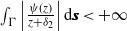
$\int_{\Gamma}\left|\frac{\psi(z)}{z+\delta_{2}}\right|{\mathrm{d}} \pmb{s}<+\infty$ and $\int_{\Gamma}\left|\frac{\psi(z)}{z-\delta_{1}}\right|{\rm e}^{b \mathrm{Re} z}{\mathrm{d}} \pmb{s}<+\infty$.












Remark 3.2. Conditions (1) and (2) ensure the boundedness and differentiability of  $f_{\Gamma}(x)$ defined as above on [0, b], and conditions (3) and (4) are required by the lemma below.
Lemma 3.2. Suppose that the rectifiable Jordan curve  $\Gamma$ is taken to satisfy the conditions (1)–(4). Then, for
 $0\leq x \leq b$,
 \begin{align}\mathcal{A}\,f_{\Gamma}(x)-\theta f_{\Gamma}(x) & = \lambda q [\,f_{\Gamma}(0)-\delta_{2}\int_{\Gamma}\frac{\psi(z)}{z+\delta_{2}}{\mathrm{d}} z]{\rm e}^{-\delta_{2}x} \nonumber \\& \quad +\lambda p\delta_{1}\left(\int_{\Gamma}\frac{\psi(z)}{z-\delta_{1}}{\rm e}^{b z}{\mathrm{d}} z\right){\rm e}^{\delta_{1}(x-b)}.\end{align}
Proof. The result can be easily derived by routine calculation (which is similar to the proof of Proposition 2 in [Reference Jacobsen and Jensen12]), where we use the condition (3) for integration by parts, and employ the relation (24) to eliminate the  $\int_{\Gamma}(\ldots){\rm e}^{xz}{\mathrm{d}} z$ term. The condition (4) guarantees that the expression (25) makes sense. The details of the derivation are omitted.
Proposition 3.3. The two linearly independent functions  $f_{i}({\cdot})$,
 $i=1,2$, introduced in Corollary 3.1 can be chosen as
 \begin{align*} f_{1}(x)=\sum_{i=1}^{3}B_{i}^{(1)}\int_{\Gamma_{i}}|\psi(z)|{\rm e}^{xz}{\mathrm{d}} z+\int_{\Gamma_{4}}|\psi(z)|{\rm e}^{xz}{\mathrm{d}} z,\quad f_{2}(x)=\sum_{i=1}^{3}B_{i}^{(2)}\int_{\Gamma_{i}}|\psi(z)|{\rm e}^{xz}{\mathrm{d}} z,\end{align*}
where
 \begin{align}\Gamma_{1}=(-\infty,-\delta_{2}),\quad \Gamma_{2}=(-\delta_{2},0),\quad \Gamma_{3}=(0,\delta_{1}), \quad \Gamma_{4}=(\delta_{1},+\infty).\end{align}
The coefficients  $(B_{1}^{(i)},B_{2}^{(i)},B_{3}^{(i)})$,
 $i=1,2,$ are unique solutions of the equation systems
 \begin{equation}\begin{split}&\left\{\begin{array}{l} \displaystyle \sum_{i=1}^{3}B_{i}\int_{\Gamma_{i}}\frac{z|\psi(z)|}{z+\delta_{2}}{\mathrm{d}} z=-\int_{\Gamma_{4}}\frac{z|\psi(z)|}{z+\delta_{2}}{\mathrm{d}} z,\\[12pt] \displaystyle \sum_{i=1}^{3}B_{i}\int_{\Gamma_{i}}\frac{|\psi(z)|}{z-\delta_{1}}{\rm e}^{bz}{\mathrm{d}} z=-\int_{\Gamma_{4}}\frac{|\psi(z)|}{z-\delta_{1}}{\rm e}^{bz}{\mathrm{d}} z, \\[12pt] \displaystyle \sum_{i=1}^{3}B_{i}\int_{\Gamma_{i}}|\psi(z)|(z-\beta\theta){\mathrm{d}} z=-\int_{\Gamma_{4}}|\psi(z)|(z-\beta\theta){\mathrm{d}} z, \end{array} \right. \\[6pt]& \left\{\begin{array}{l} \displaystyle \sum_{i=1}^{3}B_{i}\int_{\Gamma_{i}}\frac{z|\psi(z)|}{z+\delta_{2}}{\mathrm{d}} z=0,\\[12pt] \displaystyle \sum_{i=1}^{3}B_{i}\int_{\Gamma_{i}}\frac{|\psi(z)|}{z-\delta_{1}}{\rm e}^{bz}{\mathrm{d}} z=-\frac{1}{\zeta+\delta_{1}}, \\[12pt] \displaystyle \sum_{i=1}^{3}B_{i}\int_{\Gamma_{i}}|\psi(z)|(z-\beta\theta){\mathrm{d}} z=0, \end{array} \right.\end{split}\end{equation}
respectively.
Proof. It is not hard to check that the conditions (1)–(4) are satisfied with the curves given by (26) (see the discussion in [Reference Jacobsen and Jensen12, Section Reference Doney7]). Furthermore, note that  $|\psi({\cdot})|$ also satisfies (24) on each
 $\Gamma_{i}$, and consequently Lemma 3.2 holds with
 $\psi({\cdot})$ replaced by
 $|\psi({\cdot})|$ (including the replacement in the expression of
 $f_{\Gamma}({\cdot})$) and with
 $\Gamma$ replaced by
 $\Gamma_{i}$. Now for the function
 $f({\cdot})=\sum_{i=1}^{4}B_{i}\,\skew3\widehat{f}_{\Gamma_{i}}({\cdot})+Bf_{0}({\cdot})$ where
 \begin{align*}\skew3\widehat{f}_{\Gamma_{i}}(x)=\left\{\begin{array}{l@{\quad}l} \displaystyle \int_{\Gamma_{i}}|\psi(z)|{\rm e}^{xz}{\mathrm{d}} z,& 0\leq x\leq b,\\[10pt] \displaystyle 0,& x>b, \end{array} \right.\quad f_{0}(x)=\left\{\begin{array}{l@{\quad}l} \displaystyle 0,& 0\leq x\leq b,\\[5pt] \displaystyle {\rm e}^{-\zeta (x-b)},& x>b, \end{array} \right.\end{align*}
since
 \begin{align*}\mathcal{A}\,f_{0}(x)-\theta f_{0}(x)=\frac{\lambda p\delta_{1}}{\zeta+\delta_{1}}{\rm e}^{\delta_{1}(x-b)},\qquad 0\leq x\leq b,\end{align*}
we have by Lemma 3.2 that
 \begin{align*}\mathcal{A}\,f(x)-\theta f(x)&=\lambda q {\rm e}^{-\delta_{2}x}\sum_{i=1}^{4}B_{i}\int_{\Gamma_{i}}\frac{z|\psi(z)|}{z+\delta_{2}}{\mathrm{d}} z\\&\quad+\lambda p \delta_{1}{\rm e}^{\delta_{1}(x-b)}\left[\sum_{i=1}^{4}B_{i}\int_{\Gamma_{i}}\frac{|\psi(z)|}{z-\delta_{1}}{\rm e}^{bz}{\mathrm{d}} z+\frac{B}{\zeta+\delta_{1}}\right]\!, \qquad 0\leq x\leq b.\end{align*}
So if  $f({\cdot})$ satisfies (15) and (16) on [0, b], we get
 \begin{equation}\begin{cases} \displaystyle \sum_{i=1}^{4}B_{i}\int_{\Gamma_{i}}\frac{z|\psi(z)|}{z+\delta_{2}}{\mathrm{d}} z=0,\nonumber\\ \displaystyle \sum_{i=1}^{4}B_{i}\int_{\Gamma_{i}}\frac{|\psi(z)|}{z-\delta_{1}}{\rm e}^{bz}{\mathrm{d}} z+\frac{B}{\zeta+\delta_{1}}=0, \nonumber\\ \displaystyle \sum_{i=1}^{4}B_{i}\int_{\Gamma_{i}}|\psi(z)|(z-\beta\theta){\mathrm{d}} z=0.\nonumber\end{cases}\end{equation}
The rest of the proof is similar to the corresponding part in the proof of Proposition 3.1, and here we only show the nonsingularity of the coefficient matrix of the linear equation systems in (27) for fixed  $\theta>0$. Express this matrix as
 \begin{align*}\Psi=\int_{\Gamma_{3}}\int_{\Gamma_{2}}\int_{\Gamma_{1}}\begin{bmatrix} \displaystyle \frac{x_{1}|\psi(x_{1})|}{x_{1}+\delta_{2}} & \displaystyle \frac{x_{2}|\psi(x_{2})|}{x_{2}+\delta_{2}} & \displaystyle \frac{x_{3}|\psi(x_{3})|}{x_{3}+\delta_{2}} \\ \\ \displaystyle \frac{|\psi(x_{1})|}{x_{1}-\delta_{1}}{\rm e}^{x_{1}b } & \displaystyle \frac{|\psi(x_{2})|}{x_{2}-\delta_{1}}{\rm e}^{x_{2}b } & \displaystyle \frac{|\psi(x_{3})|}{x_{3}-\delta_{1}}{\rm e}^{x_{3}b } \\ \\ \displaystyle (x_{1}-\beta \theta)|\psi(x_{1})| &\displaystyle (x_{2}-\beta \theta)|\psi(x_{2})| & \displaystyle (x_{3}-\beta \theta)|\psi(x_{3})|\end{bmatrix}{\mathrm{d}} x_{1} {\mathrm{d}} x_{2} {\mathrm{d}} x_{3}.\end{align*}
One can prove that the determinant of the integrand is
 \begin{align}\frac{(R_{1,\theta}\delta_{2}\beta\theta+R_{2,\theta})\prod_{1\leq i\leq 3}|\psi(x_{i})|}{\prod_{1\leq i, j\leq 3}(\delta_{1}-x_{i})(\delta_{2}+x_{j})},\end{align}
where for each  $i=1,2$,
 $R_{i,\theta}$ has exactly the same form as
 $T_{i,\theta}$ defined in the proof of Proposition 3.1 by replacing
 $\varepsilon_{j}$ with
 $x_{j}$,
 $j=1,2,3$. It follows that, given
 $x_{i}\in \Gamma_{i}$,
 $i=1,2,3$, the value of (28) is smaller than 0, which in turn indicates that
 $\det(\Psi) \lt 0$.
Remark 3.3. We use  $|\psi({\cdot})|$ instead of
 $\psi({\cdot})$ in the proposition mainly for ease of proving the nonsingularity of the related coefficient matrix.
When  $\lambda=0$, the process Y is named the sticky reflecting OU process (without jumps). In analogy with Proposition 3.2, we obtain the Laplace transform of the first passage time in such a case.
Proposition 3.4. When  $\lambda=0$,
 \begin{align*}\mathrm{E}_{y}\left[{\rm e}^{-\theta \tau_{b}}\right]={\rm e}^{\frac{\alpha}{2\sigma^{2}}(y^{2}-b^{2})}\frac{\Lambda_{1}D_{-\frac{\theta}{\alpha}}\left(-\frac{y\sqrt{2\alpha}}{\sigma}\right)-\Lambda_{2}D_{-\frac{\theta}{\alpha}}\left(\frac{y\sqrt{2\alpha}}{\sigma}\right)}{\Lambda_{1}D_{-\frac{\theta}{\alpha}}\left(-\frac{b\sqrt{2\alpha}}{\sigma}\right)-\Lambda_{2}D_{-\frac{\theta}{\alpha}}\left(\frac{b\sqrt{2\alpha}}{\sigma}\right)}, \qquad 0\leq y\leq b,\end{align*}
where  $D_{v}({\cdot})$ denotes the parabolic cylinder function given by (see [Reference Magnus, Oberhettinger and Soni16, p. 328])
 \begin{align}D_{v}(y)=\frac{{\rm e}^{-\frac{y^{2}}{4}}}{\Gamma(-\upsilon)}\int_{0}^{+\infty}t^{-\upsilon-1}{\rm e}^{-\frac{t^{2}}{2}-yt}{\mathrm{d}} t,\end{align}
and the coefficients are
 \begin{align*}\Lambda_{1}=-\frac{\sqrt{2\alpha}}{\alpha\sigma}D_{-\frac{\theta}{\alpha}-1}\left(0\right)-\beta D_{-\frac{\theta}{\alpha}}\left(0\right)\!,\qquad \Lambda_{2}=\frac{\sqrt{2\alpha}}{\alpha\sigma}D_{-\frac{\theta}{\alpha}-1}\left(0\right)-\beta D_{-\frac{\theta}{\alpha}}\left(0\right)\!.\end{align*}
Proof. Let  $f({\cdot})=\sum_{i=1}^{2}B_{i}\,f_{\Gamma_{i}}({\cdot})$, where
 $f_{\Gamma_{i}}({\cdot})$,
 $i=1,2$, are of the form (23) with the kernel
 $\psi(z)$ replaced by
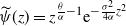 $\widetilde{\psi}(z)=z^{\frac{\theta}{\alpha}-1}{\rm e}^{-\frac{\sigma^{2}}{4\alpha}z^{2}}$ and
 $\Gamma_{i}$,
 $i=1,2$, given by
 $(0,+\infty)$ and
 $(-\infty,0)$, respectively. Direct verification yields that
 $\mathcal{A}\,f(x)-\theta f(x)=0$,
 $0\leq x\leq b$. Therefore, by Theorem 3.1 we will have (22) if
 $f({\cdot})$ meets the condition (16), or equivalently, if
 \begin{align*}\sum_{i=1}^{2}B_{i}\int_{\Gamma_{i}}\widetilde{\psi}(z)(z-\beta\theta){\mathrm{d}} z=0.\end{align*}
Now choose 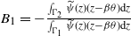 $B_{1}=-\frac{\int_{\Gamma_{2}}\widetilde{\psi}(z)(z-\beta \theta){\mathrm{d}} z}{\int_{\Gamma_{1}}\widetilde{\psi}(z)(z-\beta \theta){\mathrm{d}} z}$ and
 $B_{2}=1$, which satisfy the above equality. The conclusion then comes from (22) by virtue of the relation (29).
Acknowledgements
The authors would like to thank the editors and two anonymous referees for their valuable comments and suggestions which helped to improve the paper. This work was supported by the National Natural Science Foundation of China (grant numbers 11801407, 11631004, 71532001).


