1 Introduction
Classical risk models are typically built up based on independence assumptions. However, these assumptions may not always be appropriate in reality. There are various kinds of dependence structure proposed in literature. A common one is the level-dependent risk process which has a concrete explanation in Asmussen & Albrecher (Reference Asmussen and Albrecher2010). This could be used to model dividend payment whose amount relies on the risk reserve levels of an insurance company. Another popular dependence structure is often established between inter-claim times and successive inter-claim times or claim sizes (e.g. Albrecher & Boxma, Reference Albrecher and Boxma2004; Constantinescu et al., Reference Constantinescu, Dai, Ni and Palmowski2016). These were normally studied within a Sparre Andersen model. For instance, Albrecher & Teugels (Reference Albrecher and Teugels2006) modelled the dependence based on a copula approach, whereas Boudreault et al. (Reference Boudreault, Cossette, Landriault and Marceau2006) considered a specific mixture of the two random variables and Cheung et al. (Reference Cheung, Landriault, Willmot and Woo2010) incorporated a more general joint distribution. When the joint distribution is described using a bivariate phase-type, Badescu et al. (Reference Badescu, Cheung and Landriault2009) employed the fluid flow methodology to obtain an exact solution for the Gerber–Shiu function (Gerber & Shiu, Reference Gerber and Shiu1998) when the penalty function depends on the deficit at ruin only. More complicated dependence structure was studied under fluid flow models with applications to risk models (Badescu et al., Reference Badescu, Breuer, Da Silva Soares, Latouche, Remiche and Stanford2005; Ahn et al., Reference Ahn, Badescu and Ramaswami2007). On the other hand, dependence between the claim arrival process and the premium rate has been studied by Dubey (Reference Dubey1977), Li et al. (Reference Li, Ni and Constantinescu2015). In this paper, we would like to generalise and combine the mentioned dependence and extend to a broader dependence framework. Apart from the dependence between inter-arrival times and consecutive inter-arrival times or claim jumps, we also allow premium rates to alter according to the status of the previous and the current inter-claim times. We will analyse the model under two equivalent processes, the Markov additive process (MAP) as well as the Markov fluid flows (MFFs).
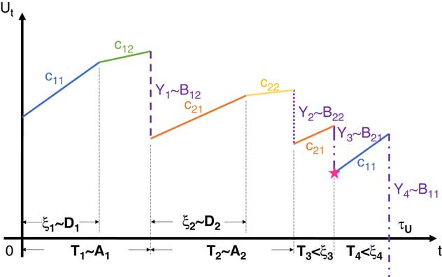
In fact, a specific dependence structure between successive inter-claim times has been constructed in Constantinescu et al. (Reference Constantinescu, Dai, Ni and Palmowski2016) in order to reflect the Bonus–Malus feature at a collective risk level. In that paper, the distribution of the current inter-claim time depends on whether the previous inter-claim time exceeds a fixed threshold which we refer here as the threshold window. We further extend that model and incorporate a more interesting dependence framework. We assume now the threshold window can be random as well and is also dependent on the status of the previous inter-arrival time. In addition, by observing both the previous and current inter-claim times and their corresponding thresholds, we let the distribution of the current claim size also follow a similar dependence rule. Furthermore, we also let premium rate vary according to the last and current inter-claim times. Figure 1 presents a visual illustration of the described framework followed by a detailed description of the model in terms of mathematical languages.
A sample path of the risk surplus process.

Let Y
k
be the size of the kth claim, T
k
the kth inter-arrival time and ξ
k
the random threshold for
 $$k\in{\Bbb N }$$
(where
 $${\Bbb N}$$
represents the set of non-negative integers). Additionally, define
 $$\overline{T} _{k} \,\colon\!{\equals}\mathop{\sum}\nolimits_{j{\equals}1}^k T_{j} $$
for
 $$k\in{\Bbb N}^{{\plus}} $$
as the kth claim arrival time (with
 $${\Bbb N}^{{\plus}} $$
the set of positive integers with the definition
 $$\overline{T} _{0} \,\colon\!{\equals}\,0$$
). The distributions of the inter-arrival time and the claim size are assumed to be continuous, and they depend on the relationship between lengths of the inter-arrival times and thresholds. Let
 $$k\in{\Bbb N}^{{\plus}} $$
and we always assume that T
0<ξ
0. The underlying dependence structure is constructed as follows:
1. The distributions of the kth inter-arrival time and the kth threshold are dependent on the relationship between the (k−1)th inter-arrival time and the (k−1)th threshold, i.e.:
a. if T k−1<ξ k−1, then T k and ξ k are distributed as A 1 and D 1, respectively,
b. otherwise, T k and ξ k are distributed as A 2 and D 2, respectively.
2. The kth claim size Y k is dependent on four environments:
a. if T k−1<ξ k−1 and T k <ξ k , then Y k is distributed as B 11,
b. if T k−1<ξ k−1 and T k ≥ξ k , then Y k is distributed as B 12,
c. if T k−1≥ξ k−1 and T k <ξ k , then Y k is distributed as B 21,
d. if T k−1≥ξ k−1 and T k ≥ξ k , then Y k is distributed as B 22.
Remark 1.1. Here A 1, A 2, D 1, D 2 and B 11, B 12, B 21 and B 22 are several given independent positive random variables. The subscript “1” represents the case T k−1<ξ k−1 and “2” represents T k−1≥ξ k−1.
Using the dependent sequences of
 $$\{ T_{k} \} _{{k\in{\Bbb N}}} $$
,
 $$\{ Y_{k} \} _{{k\in{\Bbb N}}} $$
and
 $$\{ \xi _{k} \} _{{k\in{\Bbb N}}} $$
, we can construct a stochastic process. Let {U
t
}
t≥0 be the risk surplus process at time t given by
 $$U_{t} \,\colon\!{\equals}\,u{\plus}{\int}_0^t c_{s} {\rm d}s\,{\minus}\mathop{\sum}\limits_{k{\equals}1}^{N_{t} } Y_{k} $$
where u≥0 is the initial capital, i.e. U
0=u, N
t
a counting process constructed by
 $$\{ T_{k} \} _{{k\in{\Bbb N}^{{\plus}} }} $$
, {c
s
}
s≥0 is an adapted process which takes four possible positive real numbers:
1. if T
k−1<ξ
k−1, c
s
=c
11 for
 $$s\in[\overline{T} _{{k{\minus}1}} ,\overline{T} _{{k{\minus}1}} {\plus}\xi _{k} \wedge T_{k} )$$
and c
s
=c
12 for
 $$s\in[\overline{T} _{{k{\minus}1}} {\plus}\xi _{k} \wedge T_{k} ,\overline{T} _{k} )$$
,
2. if T
k−1≥ξ
k−1, c
s
=c
21 for
 $$s\in[\overline{T} _{{k{\minus}1}} ,\overline{T} _{{k{\minus}1}} {\plus}\xi _{k} \wedge T_{k} )$$
and c
s
=c
22 for
 $$s\in[\overline{T} _{{k{\minus}1}} {\plus}\xi _{k} \wedge T_{k} ,\overline{T} _{k} )$$
.
Now define a stopping time τ U of the stochastic process {U t } t≥0 by
 $$\tau _{U} \,\colon\!{\equals}\,\inf \{ t\,\gt\,0\,\colon\,U_{t} \leq 0\} $$
The ruin probability is then defined by
 $$\psi (u)\,\colon\!{\equals}\,{\Bbb P}(\tau _{U} \,\lt\,\infty\!\mid\!U_{0} \,{\equals}\,u)$$
Remark 1.2. Note that this process is regenerative at the point marked with a star in Figure 1. We would like to study the increment X 1 of the surplus process from time 0 until the first regenerative epoch. Denote by Z (k) the kth independent variable with the same distribution as Z. Then, we separate the analysis into three cases as follows:
1. On the set (A 1<D 1), one has
 $$X_{1} \,{\equals}\,c_{{11}} A_{1} \,{\minus}\,B_{{11}} .$$
2. On the set
 $$(A_{1} \geq D_{1} )\,{\cap}\,(A_{2}^{{(1)}} \,\lt\,D_{2}^{{(1)}} )$$
, one has
 $$X_{1} \,{\equals}\,c_{{11}} D_{1} {\plus}c_{{12}} (A_{1} \,{\minus}\,D_{1} )\,{\minus}\,B_{{12}} {\plus}c_{{21}} A_{2}^{{(1)}} \,{\minus}\,B_{{21}}^{{(1)}} $$
3. On the set
 $$(A_{1} \geq D_{1} )\,{\cap}\,\big(\,{\cap}\,_{{k\,{\equals}\,1}}^{{n\,{\minus}\,1}} (A_{2}^{{(k)}} \geq D_{2}^{{(k)}} )\big)\,{\cap}\,(A_{2}^{{(n)}} \,\lt\,D_{2}^{{(n)}} )$$
where n=2,3, … , one has
 $$X_{1} \,{\equals}\,c_{{11}} D_{1} {\plus}c_{{12}} (A_{1} \,{\minus}\,D_{1} )\,{\minus}\,B_{{12}} {\plus}\mathop{\sum}\limits_{k\,{\equals}\,1}^{n\,{\minus}\,1} \left\{ {c_{{21}} D_{2}^{{(k)}} {\plus}c_{{22}} (A_{2}^{{(k)}} \,{\minus}\,D_{2}^{{(k)}} )\,{\minus}\,B_{{22}}^{{(k)}} } \right\}{\plus}c_{{21}} A_{2}^{{(n)}} \,{\minus}\,B_{{21}}^{{(n)}} $$
The second and third cases can indeed be combined by forcing the third case to be true for n=1 as well because by convention an empty intersection is defined to be the universal set. Note also that the probabilities of all the above sets sum to one. Hence, we can write the moment-generating function of X 1 as
 $${\Bbb E}[e^{{sX_{1} }} ]\,{\equals}\,{\Bbb E}\left[ {e^{{sX_{1} }} {\bf 1}_{{(A_{1} \,\lt\,D_{1} )}} } \right]{\plus}\mathop{\sum}\limits_{n\,{\equals}\,1}^\infty {\Bbb E}\left[ {e^{{sX_{1} }} {\bf 1}_{{(A_{1} \geq D_{1} )}} \left\{ {\prod\limits_{k\,{\equals}\,1}^{n\,{\minus}\,1} {\bf 1}_{{(A_{2}^{{(k)}} \geq D_{2}^{{(k)}} )}} } \right\}{\bf 1}_{{(A_{2}^{{(n)}} \,\lt\,D_{2}^{{(n)}} )}} } \right]$$
To evaluate the above expectation, consider the special case of constant thresholds with D 1=a 1 and D 2=a 2. Then, by independence we find that
 $${\Bbb E}[e^{{sX_{1} }} {\bf 1}_{{(A_{1} \,\lt\,a_{1} )}} ]\,{\equals}\,{\Bbb E}\left[ {e^{{s(c_{{11}} A_{1} \,{\minus}\,B_{{11}} )}} {\bf 1}_{{(A_{1} \,\lt\,a_{1} )}} } \right]\,{\equals}\,{\Bbb E}\left[ {e^{{sc_{{11}} A_{1} }} ;\,A_{1} \,\lt\,a_{1} } \right]{\Bbb E}\left[ {e^{{\,{\minus}\!sB_{{11}} }} } \right]$$
and for
 $$n\in{\Bbb N}^{{\plus}} $$
,
 $$\eqalignno{ &\hskip 10pt{\Bbb E}\left[ {e^{{sX_{1} }} {\bf 1}_{{(A_{1} \geq a_{1} )}} \bigg\{ \prod\limits_{k\,{\equals}\,1}^{n\,{\minus}\,1} {\bf 1}_{{(A_{2}^{{(k)}} \geq a_{2} )}} \bigg\} {\bf 1}_{{(A_{2}^{{(n)}} \,\lt\,a_{2} )}} } \right] \cr & \,{\equals}\, {\Bbb E}[e^{{s\{ c_{{11}} a_{1} {\plus}c_{{12}} (A_{1} \,{\minus}\,a_{1} )\,{\minus}\,B_{{12}} \} }} {\bf 1}_{{(A_{1} \geq a_{1} )}} ] \bigg(\prod\limits_{k\,{\equals}\,1}^{n\,{\minus}\,1} {\Bbb E}\bigg[e^{{s\{ c_{{21}} a_{2} {\plus}c_{{22}} (A_{2}^{{(k)}} \,{\minus}\,a_{2} )\,{\minus}\,B_{{22}}^{{(k)}} \} }} {\bf 1}_{{(A_{2}^{{(k)}} \geq a_{2} )}} \bigg]\bigg){\Bbb E}\bigg[e^{{s(c_{{21}} A_{2}^{{(n)}} \,{\minus}\,B_{{21}}^{{(n)}} )}} {\bf 1 }_{{(A_{2}^{{(n)}} \,\lt\,a_{2} )}} \bigg] \cr & \,{\equals}\, e^{{s(c_{{11}} \,{\minus}\,c_{{12}} )a_{1} }} {\Bbb E}[e^{{sc_{{12}} A_{1} }} ;\,A_{1} \geq a_{1} ]{\Bbb E}[e^{{\,{\minus}\!sB_{{12}} }} ]\bigg\{ \prod\limits_{k\,{\equals}\,1}^{n\,{\minus}\,1} \big(e^{{s(c_{{21}} \,{\minus}\,c_{{22}} )a_{2} }} {\Bbb E}[e^{{sc_{{22}} A_{2}^{{(k)}} }} ;\,A_{2}^{{(k)}} \geq a_{2} ]{\Bbb E}[e^{{\,{\minus}\!sB_{{22}}^{{(k)}} }} ]\big)\bigg\} \cr & \quad\quad {\times}{\Bbb E}[e^{{sc_{{21}} A_{2}^{{(n)}} }} ;\,A_{2}^{{(n)}} \,\lt\,a_{2} ]{\Bbb E}[e^{{\,{\minus}\!sB_{{21}}^{{(n)}} }} ] \cr & \,{\equals}\, e^{{s(c_{{11}} \,{\minus}\,c_{{12}} )a_{1} }} {\Bbb E}[e^{{sc_{{12}} A_{1} }} ;\,A_{1} \geq a_{1} ]{\Bbb E}[e^{{\,{\minus}\!sB_{{12}} }} ](e^{{s(c_{{21}} \,{\minus}\,c_{{22}} )a_{2} }} {\Bbb E}[e^{{sc_{{22}} A_{2} }} ;\,A_{2} \geq a_{2} ]{\Bbb E}[e^{{\,{\minus}\!sB_{{22}} }} ])^{{n\,{\minus}\,1}} \cr&\quad\quad \times {\Bbb E}[e^{{sc_{{21}} A_{2} }} ;\,A_{2} \,\lt\,a_{2} ]{\Bbb E}[e^{{\,{\minus}\!sB_{{21}} }} ] $$
Substitution of (4) and (5) into (3) yields
 $${\Bbb E}[e^{{sX_{1} }} ]\,{\equals}\,{\Bbb E}[e^{{sc_{{11}} A_{1} }} ;\,A_{1} \,\lt\,a_{1} ]{\Bbb E}[e^{{\,{\minus}\!sB_{{11}} }} ]{\plus}{{e^{{s(c_{{11}} \,{\minus}\,c_{{12}} )a_{1} }} {\Bbb E}[e^{{sc_{{12}} A_{1} }} ;\,A_{1} \geq a_{1} ]{\Bbb E}[e^{{\,{\minus}\!sB_{{12}} }} ]{\Bbb E}[e^{{sc_{{21}} A_{2} }} ;\,A_{2} \,\lt\,a_{2} ]{\Bbb E}[e^{{\,{\minus}\!sB_{{21}} }} ]} \over {1\,{\minus}\,e^{{s(c_{{21}} \,{\minus}\,c_{{22}} )a_{2} }} {\Bbb E}[e^{{sc_{{22}} A_{2} }} ;\,A_{2} \geq a_{2} ]{\Bbb E}[e^{{\,{\minus}\!sB_{{22}} }} ]}}$$
From the above expression, it will become obvious that the equation
 $${\Bbb E}[e^{{sX_{1} }} ]\,{\equals}\,1$$
coincides with the Lundberg’s equation (67) when A
1, A
2, B
11, B
12, B
21 and B
22 all conform to phase-type distributions. Notice here, however, the above identity only applies to the case with fixed thresholds. In section 2.2, we shall begin with phase-type distributed thresholds, and these will be replaced specifically by Erlang thresholds in section 3 from which Erlangisation is employed to obtain fixed thresholds at an appropriate limit.
In spite of the theoretical significance of such a dependence structure, it also makes sense in practice particularly when the modelling of systematic risks (e.g. catastrophic events) is concerned. For instance, the occurrence of a heavy snow would probably be reflected by one claim being followed by intensive claim arrivals. Let us mention two more specific examples here where the model could be applied.
Example 1.1. (Dividend payment) A company may decide to pay dividends to its shareholders only if it has a relatively safe environment. It may decide to increase the continuous dividend rate after a fixed time from the most recent claim. This fixed time is the threshold window in our model and can be 1 calendar year, for example. Specifically, we may set D 1=D 2=1 and c 11>c 12, c 21>c 22.
Example 1.2. (Reinsurance) Another example is its application in reinsurance modelling. Consider the proportional reinsurance where the retention level is r. An insurance company may be compensated if the last inter-claim time is longer than 1 year. The compensation can be reflected by the change in retention levels. More specifically, let Y be the current claim size. If the inter-arrival time from the last claim is less than 1 year, the retention rate is r 1 and we just set B 11=B 21 as r 1 Y; otherwise, the retention rate is r 2<r 1 and we set B 12=B 22 as r 2 Y.
Note that both the examples are special cases of our model and the threshold windows are normally fixed in practice. However, we would like to work with a more general framework described by Figure 1 in this paper. Although one might argue that the assumption of a random observation window seems unrealistic, we will use an Erlang random variable to approximate this fixed window. This so-called Erlangisation technique has in fact frequently appeared in literature. In risk theory context, Asmussen et al. (Reference Asmussen, Avram and Usabel2002) pioneered the approach with the purpose of approximating finite-time ruin probabilities for a classical risk model with phase-type claim sizes, and Stanford et al. (Reference Stanford, Avram, Badescu, Breuer, Da Silva Soares and Latouche2005a) employed this method in the Sparre Andersen and stationary renewal risk model cases. This approach also received popularity in the studies of fluid models (e.g. Stanford et al., Reference Stanford, Latouche, Woolford, Boychuk and Hunchak2005b). It is claimed by Ramaswami et al. (Reference Ramaswami, Woolford and Stanford2008) that the use of this technique has increased the efficiency to compute time-dependent probabilities in models of fire spread and containment. Recently, Erlangisation has also been commonly used in risk models with periodic dividend decisions to mimic deterministic checking of surplus processes (see e.g. Albrecher et al., Reference Albrecher, Cheung and Thonhauser2011; Avanzi et al., Reference Avanzi, Cheung, Wong and Woo2013).
However, the ruin probability ψ(u) defined by (2) is difficult to analyse directly. We need to first transform the process {U t } t≥0 defined by (1) to a MAP or a fluid flow process. We should mention that fluid flow processes can be only applied under the particular case where inter-arrival times, claims and thresholds follow phase-type distributions.
The structure of the paper is presented as follows. Section 2 explains how the underlying model could be transformed to a MAP as well as a fluid flow process. Section 3 returns to a more practical scenario and considers fixed threshold windows. Employing the Erlangian approximation approach, exact ruin probabilities could be obtained via proper comparison between the two related models introduced in section 2. These are then followed by a numerical example. All proofs for section 3 are collected in Appendix B.
2 Related models
2.1 MAP
The first idea is to reconstruct our problem by a MAP
 $$\{ J_{k}^{{MAP}} ,S_{k}^{{MAP}} \} _{{k\in{\Bbb N}}} $$
with two states. It is defined by
1.
 $$\{ J_{k}^{{MAP}} \} _{{k\in{\Bbb N}}} $$
is a Markov chain with two states {1,2}. For
 $$k\in{\Bbb N}$$
,
 $$J_{k}^{{MAP}} \,{\equals}\,1$$
means that the underlying inter-arrival time T
k
is less than the last threshold ξ
k
. Similarly,
 $$J_{k}^{{MAP}} \,{\equals}\,2$$
means that the last inter-arrival time T
k
is larger than or equal to the last threshold ξ
k
. Then, its transition matrix can be defined by
 $$\eqalignno{ & P\,\colon\!{\equals}\,\,\left[ {\matrix{ {p_{{11}} } & {p_{{12}} } \cr {p_{{21}} } & {p_{{22}} } \cr } } \right] \cr & \,\colon\!{\equals}\,\,\left[ {\matrix{ {{\Bbb P}(T_{k} \,\lt\,\xi _{k} \!\mid\!T_{{k\,{\minus}\,1}} \,\lt\,\xi _{{k\,{\minus}\,1}} )} & {{\Bbb P}(T_{k} \geq \xi _{k} \!\mid\!T_{{k\,{\minus}\,1}} \,\lt\,\xi _{{k\,{\minus}\,1}} )} \cr {{\Bbb P}(T_{k} \,\lt\,\xi _{k} \!\mid\!T_{{k\,{\minus}\,1}} \geq \xi _{{k\,{\minus}\,1}} )} & {{\Bbb P}(T_{k} \geq \xi _{k} \!\mid\!T_{{k\,{\minus}\,1}} \geq \xi _{{k\,{\minus}\,1}} )} \cr } } \right] \cr & \,{\equals}\,\left[ {\matrix{ {{\Bbb P}(A_{1} \,\lt\,D_{1} )} & {{\Bbb P}(A_{1} \geq D_{1} )} \cr {{\Bbb P}(A_{2} \,\lt\,D_{2} )} & {{\Bbb P}(A_{2} \geq D_{2} )} \cr } } \right] $$
2. The surplus process
 $$\{ S_{k}^{{MAP}} \} _{{k\in{\Bbb N}}} $$
governed by
 $$\{ J_{k}^{{MAP}} \} _{{k\in{\Bbb N}}} $$
is defined as
 $$S_{k}^{{MAP}} \,{\equals}\,u{\plus}\mathop{\sum}\limits_{i\,{\equals}\,1}^k Y_{i}^{{J_{{i\,{\minus}\,1}}^{{MAP}} ,J_{i}^{{MAP}} }} $$
where
 $$Y_{i}^{{j_{1} ,j_{2} }} $$
for
 $$i\in{\Bbb N}^{{\plus}} $$
and j
1, j
2∈{1,2} have independent and identical distribution as
 $$\eqalignno{ & \left[ {\matrix{ {Y_{i}^{{1,1}} } & {Y_{i}^{{1,2}} } \cr {Y_{i}^{{2,1}} } & {Y_{i}^{{2,2}} } \cr } } \right]\,\colon\!{\equals}\,\,\left[ {\matrix{ {c_{{11}} T_{i} \,{\minus}\,Y_{i} \!\mid\!T_{{i\,{\minus}\,1}} \,\lt\,\xi _{{i\,{\minus}\,1}} ,T_{i} \,\lt\,\xi _{i} } & {c_{{11}} \xi _{i} {\plus}c_{{12}} (T_{i} \,{\minus}\,\xi _{i} )\,{\minus}\,Y_{i} \!\mid\!T_{{i\,{\minus}\,1}} \,\lt\,\xi _{{i\,{\minus}\,1}} ,T_{i} \geq \xi _{i} } \cr {c_{{21}} T_{i} \,{\minus}\,Y_{i} \!\mid\!T_{{i\,{\minus}\,1}} \geq \xi _{{i\,{\minus}\,1}} ,T_{i} \,\lt\,\xi _{i} } & {c_{{21}} \xi _{i} {\plus}c_{{22}} (T_{i} \,{\minus}\,\xi _{i} )\,{\minus}\,Y_{i} \!\mid\!T_{{i\,{\minus}\,1}} \geq \xi _{{i\,{\minus}\,1}} ,T_{i} \geq \xi _{i} } \cr } } \right] \cr &\quad\quad\quad\quad\quad\quad\quad {\equals}\,\hskip-8pt\vskip-8pt^{d}\,\left[ {\matrix{ {c_{{11}} A_{1} \,{\minus}\,B_{{11}} \!\mid\!A_{1} \,\lt\,D_{1} } & {c_{{11}} D_{1} {\plus}c_{{12}} (A_{1} \,{\minus}\,D_{1} )\,{\minus}\,B_{{12}} \!\mid\!A_{1} \geq D_{1} } \cr {c_{{21}} A_{2} \,{\minus}\,B_{{21}} \!\mid\!A_{2} \,\lt\,D_{2} } & {c_{{21}} D_{1} {\plus}c_{{22}} (A_{2} \,{\minus}\,D_{2} )\,{\minus}\,B_{{12}} \!\mid\!A_{2} \geq D_{2} } \cr } } \right] $$
Remark 2.1. The positive security loading condition that ensures the surplus process drifts to positive infinity in the long run is given by (see e.g. Asmussen, Reference Asmussen2008, chapter XI, Corollary 2.9(a))
 $$\mathop{\sum}\limits_{i\,{\equals}\,1}^2 \mathop{\sum}\limits_{j\,{\equals}\,1}^2 \pi _{i} p_{{ij}} {\Bbb E}[Y^{{i,j}} ]\,\gt\,0,$$
where π 1=p 21/(p 12+p 21), and π 2=p 12/(p 12+p 21) are the stationary distribution of P and Y i,j are the generic jump distributions for i, j=1, 2. If, e.g., the thresholds are assumed to be constant such that D 1=a 1 and D 2=a 2, then one easily finds that
 $$p_{{i1}} {\Bbb E}[Y^{{i,1}} ]\,{\equals}\,{\int}_0^{a_{i} } (c_{{i1}} t\,{\minus}\,{\Bbb E}[B_{{i1}} ])f_{{A_{i} }} (t){\rm dt}$$
 $$p_{{i2}} {\Bbb E}[Y^{{i,2}} ]\,{\equals}\,{\int}_{a_{i} }^\infty \{ c_{{i2}} (t\,{\minus}\,a_{i} ){\plus}c_{{i1}} a_{i} \,{\minus}\,{\Bbb E}[B_{{i2}} ]\} f_{{A_{i} }} (t){\rm dt}$$
for i=1, 2, where
 $$f_{{A_{i} }} ( \cdot )$$
is the density of A
i
.
Define the stopping time τ
MAP
of the stochastic process
 $$\{ J_{k}^{{MAP}} ,S_{k}^{{MAP}} \} _{{k\in{\Bbb N}}} $$
by
 $$\tau ^{{MAP}} \,\colon\!{\equals}\,\,\inf \{ n\in{\Bbb N}^{{\plus}} \,\colon\,S_{n}^{{MAP}} \leq 0\} $$
The corresponding ruin probability is defined by
 $$\psi ^{{MAP}} (i,u)\,\colon\!{\equals}\,\,{\Bbb P}\left( {\tau ^{{MAP}} \,\lt\,\infty\!\mid\!(J_{0}^{{MAP}} ,S_{0}^{{MAP}} )\,{\equals}\,(i,u)} \right)$$
for i=1, 2 and u≥0. Then, we could show an equivalence in ruin probabilities between MAP and the underlying process.
Lemma 2.1. The ruin probability in (2) for the surplus process {U
t
}
t≥0 is related to that in (8) for
 $$\{ J_{k}^{{MAP}} ,S_{k}^{{MAP}} \} _{{k\in{\Bbb N}}} $$
by
 $$\psi (u)\,{\equals}\,\psi ^{{MAP}} (1,u).$$
Sketch of Proof: Note that ruin of {U
t
}
t≥0 can only occur at
 $$\overline{T} _{n} \,\colon\!{\equals}\,\,\mathop{\sum}\nolimits_{k\,{\equals}\,1}^n T_{k} $$
for
 $$n\in{\Bbb N}^{{\plus}} $$
. Define
 $$\{ U_{n}^{{\asterisk}} \} _{{n\in{\Bbb N}}} $$
by
 $$U_{n}^{{\asterisk}} \,\colon\!{\equals}\,\,U_{{\overline{T} _{n} }} $$
. Then, it is sufficient to prove that the vector
 $$[U_{1}^{{\asterisk}} ,U_{2}^{{\asterisk}} ,\,\ldots\,,U_{M}^{{\asterisk}} ]$$
given U
0=u and the vector
 $$[S_{1}^{{MAP}} ,S_{2}^{{MAP}} ,\,\ldots\,,S_{M}^{{MAP}} ]$$
given
 $$(J_{0}^{{MAP}} ,S_{0}^{{MAP}} )\,{\equals}\,(1,u)$$
have the same distribution for all
 $$M\in{\Bbb N}^{{\plus}} $$
. Without loss of generality, we only need to show one example as follows. For any real numbers u, y,
 $$\eqalignno{ &\quad {\Bbb P}(U_{1}^{{\asterisk}} \,{\minus}\,u\,\lt\,y\!\mid\!U_{0} \,{\equals}\,u,T_{0} \,\lt\,\xi _{0} ) \cr & \,{\equals}\, {\Bbb P}(c_{{11}} T_{1} \,{\minus}\,Y_{1} \,\lt\,y\!\mid\!T_{0} \,\lt\,\xi _{0} ,T_{1} \,\lt\,\xi _{1} ){\Bbb P}(T_{1} \,\lt\,\xi _{1} \!\mid\!T_{0} \,\lt\,\xi _{0} ) \cr & \quad{\plus}{\Bbb P}(c_{{12}} (T_{1} \,{\minus}\,\xi _{1} ){\plus}c_{{11}} \xi _{1} \,{\minus}\,Y_{1} \,\lt\,y\!\mid\!T_{0} \,\lt\,\xi _{0} ,T_{1} \geq \xi _{1} ){\Bbb P}(T_{1} \geq \xi _{1} \!\mid\!T_{0} \,\lt\,\xi _{0} ) \cr & \,{\equals}\, {\Bbb P}(Y_{1}^{{1,1}} \,\lt\,y){\Bbb P}(J_{1}^{{MAP}} \,{\equals}\,1\!\mid\!J_{0}^{{MAP}} \,{\equals}\,1){\plus}{\Bbb P}(Y_{1}^{{1,2}} \,\lt\,y){\Bbb P}(J_{1}^{{MAP}} \,{\equals}\,2\!\mid\!J_{0}^{{MAP}} \,{\equals}\,1) \cr & \,{\equals}\, {\Bbb P}(S_{1}^{{MAP}} \,{\minus}\,u\,\lt\,y\!\mid\!J_{0}^{{MAP}} \,{\equals}\,1,S_{0}^{{MAP}} \,{\equals}\,u) $$
2.2 MFF
Alternatively, we could describe the underlying process using a fluid flow model when the randomness conforms to phase-type distributions. The benefit of the MFF model lies in the fact that it has been extensively studied and results have been well established. It also allows for the use of the Erlangisation technique as can be seen in section 3.
In general, a phase-type random variable A~PH(α, H, h) consists of a row vector α representing the initial distribution of states, a rate matrix H (for the transient states of an underlying continuous time Markov chain), and a column vector h=−H1 (where 1 is a column vector of ones of appropriate dimension). Now let us define the state space of all phase-type random variables below:
1.
 $$D_{{\rm 1}} \mathop{\,{\equals}\,}\limits^{d} PH(\gamma _{{\rm 1}} ,\Theta _{{\rm 1}} ,\theta _{{\rm 1}} )$$
and
 $$D_{{\rm 2}} \mathop{\,{\equals}\,}\limits^{d} PH(\gamma _{{\rm 2}} ,\Theta _{{\rm 2}} ,\theta _{{\rm 2}} )$$
are of dimensions
 $$n_{{D_{1} }} $$
and
 $$n_{{D_{2} }} $$
, respectively, and the corresponding state spaces are
 $$E^{{D_{1} }} \,\colon\!{\equals}\,\,\{ 1\!^{\,\lt\,} ,2\!^{\,\lt\,} ,\,\ldots\,,(n_{{D_{1} }} )^{\,\lt\,} ,C^{\,\lt\,} \} $$
and
 $$E^{{D_{2} }} \,\colon\!{\equals}\,\{ 1^{\geq } ,2^{\geq } ,\,\ldots\,,(n_{{D_{2} }} )^{\geq } ,C^{\geq } \} $$
, where C
< and C
≥ are absorbing states.
2.
 $$A_{{\rm 1}} \mathop{\,{\equals}\,}\limits^{d} PH(\alpha _{{\rm 1}} ,H_{{\rm 1}} ,h_{{\rm 1}} )$$
is of dimension
 $$n_{{A_{1} }} $$
and has the state space
 $$E^{{A_{1} }} \,\colon\!{\equals}\,\,\{ 1_{{\plus}}^{\,\lt\,} ,2_{{\plus}}^{\,\lt\,} ,\,\ldots\,,(n_{{A_{1} }} )_{{\plus}}^{\,\lt\,} \} $$
while A
2
 $$ \mathop{\,{\equals}\,}\limits^{d} $$
PH(α
2, H
2, h
2) is of dimension
 $$n_{{A_{2} }} $$
and has the state space
 $$E^{{A_{2} }} \,\colon\!{\equals}\,\,\{ 1_{{\plus}}^{\geq } ,2_{{\plus}}^{\geq } ,\,\ldots\,,(n_{{A_{2} }} )_{{\plus}}^{\geq } \} $$
.
3.
 $$B_{{{\rm 11}}} \mathop{\,{\equals}\,}\limits^{d} PH(\beta _{{{\rm 11}}} ,G_{{{\rm 11}}} ,g_{{{\rm 11}}} )$$
,
 $$B_{{{\rm 12}}} \mathop{\,{\equals}\,}\limits^{d} PH(\beta _{{{\rm 12}}} ,G_{{{\rm 12}}} ,g_{{{\rm 12}}} )$$
,
 $$B_{{{\rm 21}}} \mathop{\,{\equals}\,}\limits^{d} PH(\beta _{{{\rm 21}}} ,G_{{{\rm 21}}} ,g_{{{\rm 21}}} )$$
and
 $$B_{{{\rm 22}}} \mathop{\,{\equals}\,}\limits^{d} PH (\beta _{{{\rm 22}}} ,G_{{{\rm 22}}} ,g_{{{\rm 22}}} )$$
are of dimensions
 $$n_{{B_{{11}} }} $$
,
 $$n_{{B_{{12}} }} $$
,
 $$n_{{B_{{21}} }} $$
and
 $$n_{{B_{{22}} }} $$
, and have the state spaces
 $$E^{{B_{{11}} }} \,\colon\!{\equals}\,\,\{ 1_{\,{\minus}\,}^{{\,\lt\,,\,\lt\,}} ,2_{\,{\minus}\,}^{{\,\lt\,,\,\lt\,}} ,\,\ldots\,,(n_{{B_{{11}} }} )_{\,{\minus}\,}^{{\,\lt\,,\,\lt\,}} \} $$
,
 $$E^{{B_{{12}} }} \,\colon\!{\equals}\,\,\{ 1_{\,{\minus}\,}^{{\,\lt\,,\geq }} ,2_{\,{\minus}\,}^{{\,\lt\,,\geq }} ,\,\ldots\,,(n_{{B_{{11}} }} )_{\,{\minus}\,}^{{\,\lt\,,\geq }} \} $$
,
 $$E^{{B_{{21}} }} \,\colon\!{\equals}\,\,\{ 1_{\,{\minus}\,}^{{\geq ,\,\lt\,}} ,2_{\,{\minus}\,}^{{\geq ,\,\lt\,}} ,\,\ldots\,,(n_{{B_{{21}} }} )_{\,{\minus}\,}^{{\geq ,\,\lt\,}} \} $$
,
 $$E^{{B_{{22}} }} \,\colon\!{\equals}\,\,\{ 1_{\,{\minus}\,}^{{\geq ,\geq }} ,2_{\,{\minus}\,}^{{\geq ,\geq }} ,\,\ldots\,,(n_{{B_{{22}} }} )_{\,{\minus}\,}^{{\geq ,\geq }} \} $$
, respectively.
Note that absorbing states are only included in the state spaces
 $$E^{{D_{1} }} $$
and
 $$E^{{D_{2} }} $$
but not the others. The reason is that when a random threshold D
1 or D
2 is “realised” (i.e. the Markov chain underlying D
1 or D
2 enters the absorbing state C
< or C
≥) before the corresponding inter-arrival time A
1 or A
2 ends, the surplus process is still going upward and the information about such states needs to be stored in the matrices. On the other hand, if A
1 or A
2 terminates before D
1 or D
2, the surplus immediately moves into a downward phase and therefore the absorbing states of A
1 or A
2 are not needed in the upcoming rate matrices. A similar reasoning could be applied to B
ij
for i, j=1, 2: once the “claim” phase ends, the surplus process immediately switches to an upward phase and the absorbing states pertaining to B
ij
will not be needed.
The process {U
t
}
t≥0 defined by (1) can be embedded to an MFF model
 $$\{ J_{t}^{{MFF}} ,R_{t}^{{MFF}} \} _{{t\geq 0}} $$
which is defined as follows.
 $$\{ J_{t}^{{MFF}} \} _{{t\geq 0}} $$
has a transition matrix Λ with the state space E=E
+∪E
−
, where
(i) E
+ is the union of the sets
 $$E^{{D_{1} }} {\times}E^{{A_{1} }} $$
and
 $$E^{{D_{2} }} {\times}E^{{A_{2} }} $$
, i.e., it contains all the state points
 $$E^{{i^{\,\lt\,} ,j_{{\plus}}^{\,\lt\,} }} $$
for
 $$i\,{\equals}\,1,2,\,\ldots\,,n_{{D_{1} }} ,C$$
and
 $$j\,{\equals}\,1,2,\,\ldots\,,n_{{A_{1} }} $$
and
 $$E^{{i^{\geq } ,j_{{\plus}}^{\geq } }} $$
for
 $$i\,{\equals}\,1,2,\,\ldots\,,n_{{D_{2} }} ,C$$
and
 $$j\,{\equals}\,1,2,\,\ldots\,,n_{{A_{2} }} $$
.
(ii) E
− is the union of sets containing the state points
 $$E^{{B_{{11}} }} $$
,
 $$E^{{B_{{12}} }} $$
,
 $$E^{{B_{{21}} }} $$
and
 $$E^{{B_{{22}} }} $$
.
Then, the transition matrix Λ of
 $$\{ J_{t}^{{MFF}} \} _{{t\geq 0}} $$
is given by
 $$\Lambda \,\colon\!{\equals}\,\,\left[ {\matrix{ {\Lambda _{{{\plus}{\plus}}} } & {\Lambda _{{{\plus}\,{\minus}\,}} } \cr {\Lambda _{{\,{\minus}\,{\plus}}} } & {\Lambda _{{\,{\minus}\,\,{\minus}\,}} } \cr } } \right]$$
where
 $$\Lambda _{{{\plus}{\plus}}} \,\colon\!{\equals}\,\,\left[ {\matrix{ {\left[ {\matrix{ {\Theta _{1} } & {\theta _{1} } \cr 0 & 0 \cr } } \right]\,\otimes\,I_{{n_{{A_{1} }} }} {\plus}I_{{n_{{D_{1} }} {\plus}1}} \,\otimes\,H_{1} } & 0 \cr 0 & {\left[ {\matrix{ {\Theta _{2} } & {\theta _{2} } \cr 0 & 0 \cr } } \right]\,\otimes\,I_{{n_{{A_{2} }} }} {\plus}I_{{n_{{D_{2} }} {\plus}1}} \,\otimes\,H_{2} } \cr } } \right]$$
 $$\Lambda _{{{\plus}\,{\minus}\,}} \,\colon\!{\equals}\,\,\left[ {\matrix{ {\left[ {\matrix{ {\beta _{{11}} \,\otimes\,{ 1}_{{n_{{D_{1} }} }} \,\otimes\,h_{1} } & 0 \cr 0 & {\beta _{{12}} \,\otimes\,h_{1} } \cr } } \right]} & 0 \cr 0 & {\left[ {\matrix{ {\beta _{{21}} \,\otimes\,{ 1}_{{n_{{D_{2} }} }} \,\otimes\,h_{2} } & 0 \cr 0 & {\beta _{{22}} \,\otimes\,h_{2} } \cr } } \right]} \cr } } \right]$$
 $$\Lambda _{{\,{\minus}\,{\plus}}} \,\colon\!{\equals}\,\,\left[ {\matrix{ {g_{{11}} \,\otimes\,[\gamma _{1} ,0]\,\otimes\,\alpha _{1} } & 0 \cr 0 & {g_{{12}} \,\otimes\,[\gamma _{2} ,0]\,\otimes\,\alpha _{2} } \cr {g_{{21}} \,\otimes\,[\gamma _{1} ,0]\,\otimes\,\alpha _{1} } & 0 \cr 0 & {g_{{22}} \,\otimes\,[\gamma _{2} ,0]\,\otimes\,\alpha _{2} } \cr } } \right]$$
 $$\Lambda _{{\,{\minus}\,\,{\minus}\,}} \,\colon\!{\equals}\,\,\left[ {\matrix{ {G_{{11}} } & 0 & 0 & 0 \cr 0 & {G_{{12}} } & 0 & 0 \cr 0 & 0 & {G_{{21}} } & 0 \cr 0 & 0 & 0 & {G_{{22}} } \cr } } \right],$$
with I
m
the identity matrix of dimension m and 1
m
a column vector of ones of dimension m. It is understood that 0 in (9)–(12) is a zero matrix of appropriate dimension (and similarly sometimes we shall simply use I to represent an identity matrix when the dimension is clear from the context). Finally, an MFF process
 $$\{ R_{t}^{{MFF}} \} _{{t\geq 0}} $$
can be constructed as
 $$R_{t}^{{MFF}} \,{\equals}\,u{\plus}{\int}_0^t c(J_{s}^{{MFF}} ){\rm d}s$$
where 1. c(m)=c
11 for
 $$m\,{\equals}\,E^{{i^{\,\lt\,} ,j_{{\plus}}^{\,\lt\,} }} $$
for
 $$i\,{\equals}\,1,2,\,\ldots\,,n_{{D_{1} }} $$
and
 $$j\,{\equals}\,1,2,\,\ldots\,,n_{{A_{1} }} $$
;
2. c(m)=c
12 for
 $$m\,{\equals}\,E^{{i^{\,\lt\,} ,j_{{\plus}}^{\,\lt\,} }} $$
for i=C and
 $$j\,{\equals}\,1,2,\,\ldots\,,n_{{A_{1} }} $$
;
3. c(m)=c
21 for
 $$m\,{\equals}\,E^{{i^{\geq } ,j_{{\plus}}^{\geq } }} $$
for
 $$i\,{\equals}\,1,2,\,\ldots\,,n_{{D_{2} }} $$
and
 $$j\,{\equals}\,1,2,\,\ldots\,,n_{{A_{2} }} $$
;
4. c(m)=c
22 for
 $$m\,{\equals}\,E^{{i^{\geq } ,j_{{\plus}}^{\geq } }} $$
for i=C and
 $$j\,{\equals}\,1,2,\,\ldots\,,n_{{A_{2} }} $$
;
5. c(m)= − 1 for m∈E −.
Define the stopping time and the corresponding ruin probability as
 $$\eqalignno{ & \tau ^{{MFF}} \,\colon\!{\equals}\,\,\inf \{ t\,\gt\,0\,\colon\,R_{t}^{{MFF}} \leq 0\} \cr & \psi _{{i,j}}^{{MFF}} (u)\,\colon\!{\equals}\,\,{\Bbb P}(\tau ^{{MFF}} \,\lt\,\infty,J_{{\tau ^{{MFF}} }}^{{MFF}} \,{\equals}\,j\!\mid\!(J_{0}^{{MFF}} ,R_{0}^{{MFF}} )\,{\equals}\,(i,u)) $$
for i∈E + and j∈E −. Then, we can write this as the n +×n − matrix
 $$\Psi (u)\,\colon\!{\equals}\,\,\{ \psi _{{i,j}}^{{MFF}} (u)\} _{{(i,j)\in E^{{\plus}} {\times}E^{\,{\minus}\,} }} $$
with
 $$n_{{\plus}} \,\colon\!{\equals}\,\,(n_{{D_{1} }} {\plus}1)n_{{A_{1} }} {\plus}(n_{{D_{2} }} {\plus}1)n_{{A_{2} }} $$
and
 $$n_{\,{\minus}\,} \,\colon\!{\equals}\,\,n_{{B_{{11}} }} {\plus}n_{{B_{{12}} }} {\plus}n_{{B_{{21}} }} {\plus}n_{{B_{{22}} }} $$
.
According to Asmussen (Reference Asmussen1995, theorem 3.2), we can solve the characteristic equation to obtain Ψ(u) whose ijth element is defined by (13). Note that Ψ(0) represents the probability of this process down-crossing level 0 for the first time when it initially starts from 0 in an upward phase. Similar to the well-known Riccati equation shown in the MFF literature, we could also state the following lemma.
Lemma 2.2. (Asmussen et al., Reference Asmussen, Avram and Usabel2002, theorem 2) Let Ψ0:=Ψ(0). Ψ0 satisfies the Riccati equation
 $$\Lambda _{{{\plus}\,{\minus}\,,c}} {\plus}\Lambda _{{{\plus}{\plus},c}} \Psi _{0} {\plus}\Psi _{0} \Lambda _{{\,{\minus}\,\,{\minus}\,}} {\plus}\Psi _{0} \Lambda _{{\,{\minus}\,{\plus}}} \Psi _{0} \,{\equals}\,0,$$
where
 $$\eqalignno{ & \Lambda _{{{\plus}{\plus},c}} \,\colon\!{\equals}\,\,\left[ {\matrix{ {\left[ {\matrix{ {{1 \over {c_{{11}} }}\Theta _{1} } & {{1 \over {c_{{11}} }}\theta _{1} } \cr 0 & 0 \cr } } \right]\,\otimes\,I_{{n_{{A_{1} }} }} {\plus}\left[ {\matrix{ {{1 \over {c_{{11}} }}I_{{n_{{D_{1} }} }} } & 0 \cr 0 & {{1 \over {c_{{12}} }}} \cr } } \right]\,\otimes\,H_{1} } &\hskip-21pt 0 \cr 0 &\hskip-45pt {\left[ {\matrix{ {{1 \over {c_{{21}} }}\Theta _{2} } & {{1 \over {c_{{21}} }}\theta _{2} } \cr 0 & 0 \cr } } \right]\,\otimes\,I_{{n_{{A_{2} }} }} {\plus}\left[ {\matrix{ {{1 \over {c_{{21}} }}I_{{n_{{D_{2} }} }} } & 0 \cr 0 & {{1 \over {c_{{22}} }}} \cr } } \right]\,\otimes\,H_{2} } \cr } } \right] \cr & \Lambda _{{{\plus}\,{\minus}\,,c}} \,\colon\!{\equals}\,\,\left[ {\matrix{ {\left[ {\matrix{ {{1 \over {c_{{11}} }}(\beta _{{11}} \,\otimes\,{ 1}_{{n_{{D_{1} }} }} \,\otimes\,h_{1} )} & 0 \cr 0 & {{1 \over {c_{{12}} }}(\beta _{{12}} \,\otimes\,h_{1} )} \cr } } \right]} & 0 \cr 0 & {\left[ {\matrix{ {{1 \over {c_{{21}} }}(\beta _{{21}} \,\otimes\,{ 1}_{{n_{{D_{2} }} }} \,\otimes\,h_{2} )} & 0 \cr 0 & {{1 \over {c_{{22}} }}(\beta _{{22}} \,\otimes\,h_{2} )} \cr } } \right]} \cr } } \right]. $$
In addition, the matrix ruin probability (14) can be represented as
 $$\Psi (u)\,{\equals}\,\Psi _{0} e^{{\Gamma u}} $$
for u ≥ 0, where Γ:=Λ−−+Λ−+Ψ0.
Interested readers are referred to, e.g. Ahn & Ramaswami (Reference Ahn and Ramaswami2005) and Bean et al. (Reference Bean, O'Reilly and Taylor2005) and for efficient algorithms to compute Ψ0. The ruin probabilities for our model can now be readily connected to those for the MFF model by comparing the two processes.
Corollary 2.1. The ruin probability in (2) for the surplus process {U t } t≥0 is given by
 $$\psi (u)\,{\equals}\,[\gamma _{1} \,\otimes\,\alpha _{1} ,0]\Psi (u){ 1}_{{n_{\,{\minus}\,} }} $$
for u≥0, where 0 here is a zero row vector of dimension
 $$n_{{A_{1} }} {\plus}(n_{{D_{2} }} {\plus}1)n_{{A_{2} }} $$
.
3 Fixed threshold windows
In this section, we explicitly derive he ruin probability ψ(u) defined by (2) when the thresholds D 1 and D 2 are both fixed. Let a 1 and a 2 be two positive real numbers. In the sequel, we suppose that
1. the inter-arrival time distribution
 $$A_{i} \mathop{\,{\equals}\,}\limits^{d} PH(\alpha _{i} ,H_{i} ,h_{i} ),$$
2. the claim size distribution
 $$B_{{ij}} \mathop{\,{\equals}\,}\limits^{d} PH(\beta_{{ij}} ,G_{{ij}} ,g_{{ij}} ),$$
3. D i =a i .
for i, j∈{1,2}. Note that only the third distributional assumption is different from section 2.2. Then, we denote the underlying process by
 $$\{ U_{t}^{{fix}} \} _{{t\geq 0}} $$
as a special case of (1). Similarly, the corresponding MAP can be written as
 $$\{ J_{k}^{{(MAP,fix)}} ,S_{k}^{{(MAP,fix)}} \} _{{k\in{\Bbb N}}} $$
. It was demonstrated in Lemma 2.1 that the ruin probabilities for
 $$\{ U_{t}^{{fix}} \} _{{t\geq 0}} $$
and
 $$\{ J_{k}^{{(MAP,fix)}} ,S_{k}^{{(MAP,fix)}} \} _{{k\in{\Bbb N}}} $$
are equivalent.
We shall be using the Erlangisation technique to approximate those fixed thresholds, and the exact results can be obtained by taking appropriate limits. In particular, we replace the fixed thresholds D 1 and D 2 by independent and identically distributed sequences of thresholds as
 $$D_{1}^{{(n)}} \mathop{\,{\equals}\,}\limits^{d} {\rm Erlang}\left( {n,{n \over {a_{1} }}} \right)\:\;{\rm and}\;\:D_{2}^{{(n)}} \mathop{\,{\equals}\,}\limits^{d} {\rm Erlang}\left( {n,{n \over {a_{2} }}} \right)$$
Analogously, the resulting surplus process is
 $$\{ U_{t}^{{(n)}} \} _{{t\geq 0}} $$
with corresponding MAP given by
 $$\{ J_{k}^{{(MAP,n)}} ,S_{k}^{{(MAP,n)}} \} _{{k\in{\Bbb N}}} $$
. Furthermore, the assumption that
 $$D_{1}^{{(n)}} $$
and
 $$D_{2}^{{(n)}} $$
conform to Erlang distributions allows us to also describe the process using a fluid flow model (say
 $$\{ J_{t}^{{(MFF,n)}} ,R_{t}^{{(MFF,n)}} \} _{{t\geq 0}} $$
). It has been proved by Lemma 2.1 and Corollary 2.1 that the ruin probabilities of these three models are closely connected with each other. Let us introduce some other notations which will be used later.
1. ψ
fix
(u) and ψ
n
(u) correspond to the ruin probabilities of
 $$\{ U_{t}^{{fix}} \} _{{t\geq 0}} $$
and
 $$\{ U_{t}^{{(n)}} \} _{{t\geq 0}} $$
, respectively, with the definition given by (2).
2. ψ
(MAP,fix) (i,u) and
 $$\psi _{n}^{{MAP}} (i,u)$$
are the ruin probabilities of
 $$\{ J_{k}^{{(MAP,fix)}} ,S_{k}^{{(MAP,fix)}} \} _{{k\in{\Bbb N}}} $$
and
 $$\{ J_{k}^{{(MAP,n)}} ,S_{k}^{{(MAP,n)}} \} _{{k\in{\Bbb N}}} $$
, respectively, defined via (8).
First, we show that the ruin probabilities under the fixed thresholds scenario could be approximated using a sequence of those derived by Erlang distributed threshold windows.
Lemma 3.1. The ruin probability under fixed threshold windows can be obtained as the limit of the Erlangisation approximation such that
 $$\mathop {\lim }\limits_{n\to\infty} \psi _{n} (u)\,{\equals}\,\psi ^{{fix}} (u)$$
for u≥0.
Proof. See Appendix B.1.
Recalling the equivalence between ψ
fix
(u) and ψ
(MAP,fix) (1,u) from Lemma 2.1, it is now sufficient to analyse the latter ruin probability. Furthermore, in order to approximate using MFF process, we could construct a matrix consisting of the ruin probability for
 $$\{ J_{k}^{{(MAP,fix)}} ,S_{k}^{{(MAP,fix)}} \} _{{k\in{\Bbb N}}} $$
as follows. Define
 $$\eqalign { &\psi _{i}^{{(MAP,fix)}} (u,j,k)\,\cr & \colon{\equals}\,\, {\Bbb P}\big((\tau ^{{(MAP,fix)}} \,\lt\,\infty)\,{\cap}\,(e_{Y} (\tau ^{{(MAP,fix)}} )\,{\equals}\,k)\!\mid\!((J_{0}^{{(MAP,fix)}} ,S_{0}^{{(MAP,fix)}} )\, {\equals}\,(i,u))\,{\cap}\,(e_{T} (0)\,{\equals}\,j)\big)$$
where i=1, 2;
 $$j\in E^{{A_{i} }} $$
; k∈E
− and e
T
(0) and e
Y
(τ
(MAP,fix) ), respectively, represent the initial state of the first inter-arrival time T
1 and the state (in the fluid equivalent) when down-crossing zero by the claim causing ruin at the ruin time τ
(MAP,fix) . Then, we shall rewrite it in the matrix form as
 $$\Psi _{i}^{{(MAP,fix)}} (u)\,{\equals}\,\{ \psi _{i}^{{(MAP,fix)}} (u,j,k)\} _{{(j,k)\in E^{{A_{i} }} {\times}E^{\,{\minus}\,} }} $$
for i=1, 2. Combining the result demonstrated in Corollary 2.1, we are now ready to present the main theorem for ruin probability computation.
Theorem 3.1. Let
 $$\Xi \,\colon\!{\equals}\,\,\left[ {\matrix{ {(g_{{11}} \alpha _{1} )\Psi _{1}^{{(MAP,fix)}} (0)} \cr {(g_{{12}} \alpha _{2} )\Psi _{2}^{{(MAP,fix)}} (0)} \cr {(g_{{21}} \alpha _{1} )\Psi _{1}^{{(MAP,fix)}} (0)} \cr {(g_{{22}} \alpha _{2} )\Psi _{2}^{{(MAP,fix)}} (0)} \cr } } \right].$$
Then, the ruin probability under fixed threshold windows is given by
 $$\psi ^{{fix}} (u)\,{\equals}\,\eta e^{{(\Lambda _{{\,{\minus}\,\,{\minus}\,}} {\plus}\Xi )u}} 1_{{n_{\,{\minus}\,} }} $$
for u ≥ 0, where
 $$\eta \,\colon\!{\equals}\,\,\alpha _{1} \Psi _{1}^{{(MAP,fix)}} (0)$$
and Λ−− is given by (12).
Proof. See Appendix B.2.
It is instructive to note that the solution ψ
fix
(u) in (19) depends on
 $$\Psi _{1}^{{(MAP,fix)}} (0)$$
and
 $$\Psi _{2}^{{(MAP,fix)}} (0)$$
via Ξ. The following lemma gives a further relationship between Ξ and
 $$\Psi _{1}^{{(MAP,fix)}} (0)$$
as well as
 $$\Psi _{2}^{{(MAP,fix)}} (0)$$
.
Lemma 3.2. The components of
 $$\Psi _{1}^{{(MAP,fix)}} (0)$$
and
 $$\Psi _{2}^{{(MAP,fix)}} (0)$$
can be represented in the vectorisation form
 $${\rm vec}(\Psi _{1}^{{(MAP,fix)}} (0))\,{\equals}\,\,{\minus}\,(I\,{\minus}\,{\rm exp}(a_{1} c_{{11}} Q_{{11}} ))Q_{{11}}^{{\,{\minus}\!1}} {\rm vec}(C_{{11}} )\,{\minus}\,{\rm exp}(a_{1} c_{{11}} Q_{{11}} )Q_{{12}}^{{\,{\minus}\!1}} {\rm vec}(C_{{12}} )$$
 $${\rm vec}(\Psi _{2}^{{(MAP,fix)}} (0))\,{\equals}\,\,{\minus}\,(I\,{\minus}\,{\rm exp}(a_{2} c_{{22}} Q_{{21}} ))Q_{{21}}^{{\,{\minus}\!1}} {\rm vec}(C_{{21}} )\,{\minus}\,{\rm exp}(a_{2} c_{{21}} Q_{{21}} )Q_{{22}}^{{\,{\minus}\!1}} {\rm vec}(C_{{22}} )$$
where vec(X) denotes a column vector consisting of columns of matrix X, and the matrices C ij and Q ij for i, j=1, 2 are defined by
 $$C_{{11}} \,\colon\!{\equals}\,\left[ {\matrix{ {\beta _{{11}} \,\otimes\,h_{1} } & {0_{{n_{{A_{1} }} {\times}n_{{B_{{12}} }} }} } & {0_{{n_{{A_{2} }} {\times}n_{{B_{{21}} }} }} } & {0_{{n_{{A_{2} }} {\times}n_{{B_{{22}} }} }} }\!\cr } } \right]\,/\,c_{{11}} $$
 $$C_{{12}} \,\colon\!{\equals}\,\left[ {\matrix{ {0_{{n_{{A_{1} }} {\times}n_{{B_{{11}} }} }} } & {\beta _{{12}} \,\otimes\,h_{1} } & {0_{{n_{{A_{2} }} {\times}n_{{B_{{21}} }} }} } & {0_{{n_{{A_{2} }} {\times}n_{{B_{{22}} }} }} }\!\cr } } \right]\,/\,c_{{12}} $$
 $$C_{{21}} \,\colon\!{\equals}\,\left[ {\matrix{ {0_{{n_{{A_{1} }} {\times}n_{{B_{{11}} }} }} } & {0_{{n_{{A_{1} }} {\times}n_{{B_{{12}} }} }} } & {\beta _{{21}} \,\otimes\,h_{2} } & {0_{{n_{{A_{2} }} {\times}n_{{B_{{22}} }} }} }\!\cr } } \right]\,/\,c_{{21}} $$
 $$C_{{22}} \,\colon\!{\equals}\,\left[ {\matrix{ {0_{{n_{{A_{1} }} {\times}n_{{B_{{11}} }} }} } & {0_{{n_{{A_{1} }} {\times}n_{{B_{{12}} }} }} } & {0_{{n_{{A_{2} }} {\times}n_{{B_{{21}} }} }} } & {\beta _{{22}} \,\otimes\,h_{2} }\!\cr } } \right]\,/\,c_{{22}} $$
 $$Q_{{ij}} \,\colon\!{\equals}\,\,(\Lambda _{{\,{\minus}{\minus}\,}}^{T} {\plus}\Xi ^{T} )\,\oplus\,{{H_{i} } \over {c_{{ij}} }}$$
and
 $$0_{{m_{1} {\times}m_{2} }} $$
is a zero matrix of dimension m
1×m
2.
Proof. See Appendix B.3.
Lemma 3.2 indicates that we could derive
 $$\Psi _{1}^{{(MAP,fix)}} (0)$$
and
 $$\Psi _{2}^{{(MAP,fix)}} (0)$$
from Ξ as Q
ij
for i, j=1, 2 depend on Ξ. Therefore, we shall propose an algorithm to compute Ξ. Recall that H
i
is the infinitesimal generator of the phase-type distributed A
i
for i=1, 2. In what follows, it is assumed that each H
i
can be decomposed via diagonalisation by
 $$H_{i} \,{\equals}\,V_{i} K_{i} V_{i}^{{\,{\minus}\!1}} $$
where K i is a diagonal matrix. We first prove the following theorem.
Theorem 3.2. Suppose that s satisfies Re(s)<0 and s is not an eigenvalue of G
ij
for any i, j=1, 2. Assume that the matrix Λ−− + Ξ (or
 $$\Lambda _{{\,{\minus}{\minus}\,}}^{T} {\plus}\Xi ^{T} $$
) is diagonalisable. Then s is the eigenvalue of the matrix Λ−− + Ξ if and only if
 $$(P_{{11}} (s){\plus}Z_{{11}} (s))(P_{{22}} (s){\plus}Z_{{22}} (s))Z_{{12}} (s)Z_{{21}} (s)\,{\equals}\,Z_{{11}} (s)P_{{12}} (s)P_{{21}} (s)Z_{{22}} (s)$$
where, for i, j=1, 2
 $$P_{{i1}} (s)\,\colon\!{\equals}\,\, \alpha _{i} V_{i} \left( {I\,{\minus}\,{\rm exp}\left( {a_{i} c_{{i1}} \left( {sI{\plus}{{K_{i} } \over {c_{{i1}} }}} \right)} \right)} \right)\left( {sI{\plus}{{K_{i} } \over {c_{{i1}} }}} \right)^{{\!\!{\minus}\!1}} V_{i}^{{\,{\minus}\!1}} h_{i} $$
 $$P_{{i2}} (s)\,\colon\!{\equals}\,\, \alpha _{i} V_{i} {\rm exp}\left( {a_{i} c_{{i1}} \left( {sI{\plus}{{K_{i} } \over {c_{{i1}} }}} \right)} \right)\left( {sI{\plus}{{K_{i} } \over {c_{{i2}} }}} \right)^{{\!\!{\minus}\!1}} V_{i}^{{\,{\minus}\!1}} h_{i} $$
 $$Z_{{ij}} (s)\,\colon\!{\equals}\,\, {{c_{{ij}} } \over {\beta _{{ij}} (sI\,{\minus}\,G_{{ij}} )^{{\,{\minus}\!1}} g_{{ij}} }}$$
Furthermore, the corresponding (right) eigenvector of Λ––+ Ξ is
 $$v(s)\,\colon\!{\equals}\,\,\left[ {\matrix{ {(sI\,{\minus}\,G_{{11}} )^{{\,{\minus}\,1}} g_{{11}} a(s)} \cr {(sI\,{\minus}\,G_{{12}} )^{{\,{\minus}\,1}} g_{{12}} } \cr {(sI\,{\minus}\,G_{{21}} )^{{\,{\minus}\,1}} g_{{21}} a(s)} \cr {(sI\,{\minus}\,G_{{22}} )^{{\,{\minus}\,1}} g_{{22}} } \cr } } \right]$$
where a(s):= − (P 12(s)Z 11(s))/((P 11(s)+Z 11(s))Z 12(s)).
Proof. See Appendix B.4.
Remark 3.1. Indeed, equation (28) coincides with equation (67) which is the Lundberg’s equation for the present model. See Corollary C.2.
Using the roots obtained in the above theorem, we are able to compute Ξ as follows:
Corollary 3.1. Assume that there exists n
− distinct roots of (28) with negative real part. These roots are denoted by
 $$\kappa _{1} ,\kappa _{2} ,\,\ldots\,,\kappa _{{n_{\,{\minus}\,} }} $$
, and are assumed not to coincide with the eigenvalues of G
ij
for any i, j=1, 2. Their corresponding (right) eigenvectors are
 $$v_{1} ,v_{2} ,\,\ldots\,,v_{{n_{\,{\minus}\,} }} $$
defined via (32) as v
i
:=v(κ
i
) for i=1, 2, … ,n
−. Then, Ξ can be calculated as
 $$\Xi \,{\equals}\,\left[ {\matrix{ {v_{1} ,v_{2} ,\,\ldots\,,v_{{n_{\,{\minus}\!\!} }} } \cr } } \right]\left[ {\matrix{ {\kappa _{1} } & {} & {} & {} \cr {} & {\kappa _{2} } & {} & {} \cr {} & {} & \ddots & {} \cr {} & {} & {} & {\kappa _{{n_{\,{\minus}\,} }} } \cr } } \right]\left[ {\matrix{ {v_{1} ,v_{2} ,\,\ldots\,,v_{{n_{\,{\minus}\,} }} } \cr } } \right]^{{\,{\minus}\,1}} \,{\minus}\,\Lambda _{{\,{\minus}\,\,{\minus}\,}} .$$
Proof. See Appendix B.4.
4 Numerical example
Here we present one numerical example showing how explicit solution of ψ fix (u) can be calculated using the methodology developed.
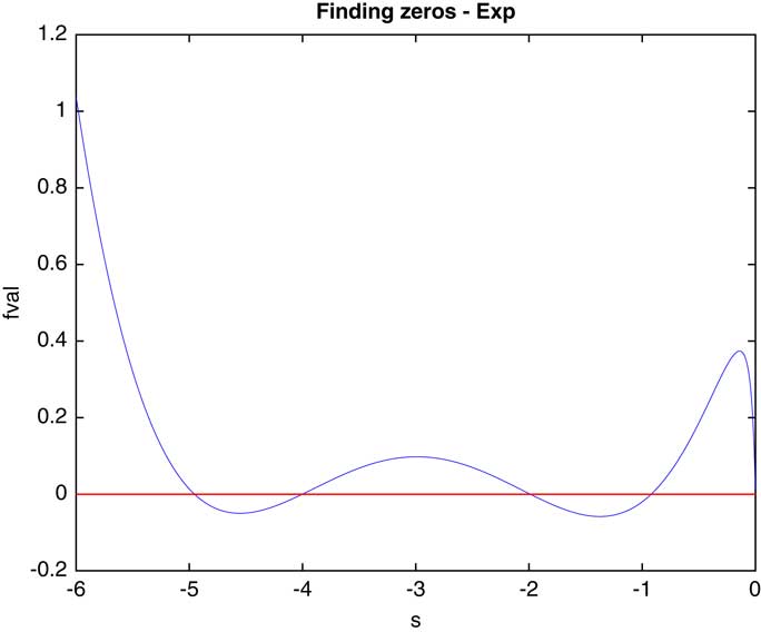
Example 4.1 . Let the premium rates be c 11=c 12=c 21=c 22=1. The inter-arrival times are A 1~Exp(0.05) and A 2~Exp(1) while the claim distributions are B 11~Exp(5), B 12~Exp(4), B 21~Exp(2) and B 22~Exp(1). The threshold windows are assumed to be fixed at D 1=0.5 and D 2=1. Then, there exists four negative real roots
 $$\left[ {\matrix{ {\kappa _{1} } & {\kappa _{2} } & {\kappa _{3} } & {\kappa _{4} } \cr } } \right]\,{\equals}\,\left[ {\matrix{ {\,{\minus}\,4.9541} & {\,{\minus}\,4.0014} & {\,{\minus}\,1.9887} & {\,{\minus}\,0.9210} \cr } } \right].$$
Figure 2 visually shows these four distinct roots as the result of solving (28).
Finding zeros.

Subsequently, using (32), we write down the matrix of the (right) eigenvectors and then, since the four roots are distinct, by Corollary 3.1, we have
 $$\Xi \,{\equals}\,\left[ {\matrix{ {0.0460} & {0.0083} & {0.0276} & {0.0155} \cr {0.0004} & {0.0009} & {1.3474} & {0.3076} \cr {0.0184} & {0.0033} & {0.0110} & {0.0062} \cr {0.0001} & {0.0002} & {0.3369} & {0.0769} \cr } } \right]$$
Using Lemma 3.2, we can calculate
 $$\Psi _{1}^{{(MAP,fix)}} (0)\,{\equals}\,\left[ {\matrix{ {0.0326} & {0.0029} & {0.0200} & {0.0138} \cr } } \right]$$
Finally, based on Theorem 3.1, the ruin probability is
 $$\eqalignno{ \psi ^{{fix}} \,(u)\,&{\equals}\, \left {\alpha _{1} \,\Psi _{1} ^{{(MAP,fix)}} (0)\,{\rm exp}\,((\Lambda {\,_{\minus}{_\minus}}} \,{\plus}\,\Xi )\,u){ 1}_{{n_{\,{\minus}\,} }} } \right. \cr &\,{\equals}\,0.0{\rm 323}\,e^{{\,{\minus}\!{\rm 4}.{\rm 9541}u}} \,{\plus}\,0.0{\rm 153}\,e^{{\,{\minus}\!{\rm 4}.00{\rm 14}u}} \,{\plus}\,0.0{\rm 199}\,e^{{\,{\minus}\,{\rm 1}.{\rm 9887}u}} \,{\plus}0.0{\rm 119}\,e^{{\,{\minus}\!0.{\rm 921}0u}} $$
5 Conclusion
In this paper, we have established a generalised dependence framework within a Sparre Andersen model. The dependence structure relies ultimately on a comparison between the recent two consecutive inter-claim times and their corresponding threshold windows. Both inter-arrival times and threshold windows are random variables and their distributions are determined by the current status. The current status can be described by a continuous time Markov process with only two states whose transition is reflected by the above mentioned dependence framework. Furthermore, we connect such dependence with the claim size distributions and the premium rates as well. Recall Figure 1 for a sample path of the process.
Then this process can be identified by two embedded models, namely the MAP and the MFF. It can be proved that the ruin probabilities for these proxy models are the same as those under concern. The use of the MFF model could even allow us to compute in an exact form the ruin probabilities when the threshold windows are fixed, thanks to the Erlangian approximation technique. This method first approximates fixed observation windows by Erlang(n) random variables. Then the equivalence of ruin probabilities at the limit and those for a process with fixed threshold window can be verified. In addition, we also explain an algorithm to calculate initial values and the exponent terms. This was illustrated also in a numerical example.
Possible future research could be consideration of a more complex dependence structure. Instead of observing whether inter-claim time is larger or smaller than their corresponding thresholds, it would be interesting to look at which interval it belongs to when the threshold windows are divided into several layers. Alternatively, a multi-period dependence could be introduced. That is to say, we could add dependence further ahead by taking into account of a few previous inter-claim times. Of course these extensions would complicate the model dramatically, yet solutions are expected to be obtainable via a similar approach.
Acknowledgements
Eric Cheung acknowledges the support from the Research Grants Council of the Hong Kong Special Administrative Region (Project Number: 17324016). The authors would like to thank the anonymous reviewers for their useful suggestions that improved the quality of the paper.
Appendix
A Kronecker product and sum
This section demonstrates preliminary knowledge about the Kronecker product and sum. The Kronecker product ⊗ is defined by
 $$A\,\otimes\,B\,\colon\!{\equals}\,\,\left[ {\matrix{ {A_{{11}} B} & {A_{{12}} B} & \cdots & {A_{{1m}} B} \cr {A_{{21}} B} & {A_{{22}} B} & {} & {A_{{2m}} B} \cr \vdots & {} & \ddots & \vdots \cr {A_{{n1}} B} & {A_{{n2}} B} & \cdots & {A_{{nm}} B} \cr } } \right]$$
where A and B are two matrices and A has a dimension m×n with ijth element A ij . On the other hand, for square matrices A and B of dimensions n A and n B , respectively, ⊕ denotes a Kronecker sum whose definition is given by
 $$A\,\oplus\,B\,\colon\!{\equals}\,\,A\,\otimes\,I_{{n_{B} }} {\plus}I_{{n_{A} }} \,\otimes\,B$$
where I n is the identity matrix with dimension n. The following lemma states some well-known properties of the Kronecker product and sum which will be used throughout the paper.
Lemma A.1. When the dimensions of the involved matrices make sense, the following properties hold true:
1. exp(A)⊗exp(B)=exp(A⊕B).
2. (A⊗C)(B⊗D)=(AB)⊗(CD).
3. (A⊗B)−1=A −1⊗B −1.
4. If AX+XB+C=0, then (B T ⊕A)vec(X)+vec(C)=0, where vec(X) is the vectorisation of X.
5. If A and B has a diagonalised form
 $$A\,{\equals}\,V_{A} D_{A} V_{A}^{{\,{\minus}\,1}} $$
and
 $$B\,{\equals}\,V_{B} D_{B} V_{B}^{{\,{\minus}\,1}} $$
where D
A
and D
B
are diagonal matrices, then
 $$A\,\oplus\,B\,{\equals}\,(V_{A} \,\otimes\,V_{B} )(D_{A} \,\oplus\,D_{B} )(V_{A}^{{\,{\minus}\,1}} \,\otimes\,V_{B}^{{\,{\minus}\,1}} )$$
can also be represented in a diagonalised form.
B. Proofs of section 3
B.1. Proof of Lemma 3.1
First, in order to conduct the proof we need the following lemma which is available from Jagerman (Reference Jagerman1982, equation (2)) and Jagerman (Reference Jagerman1978, theorem 1).
Lemma B.1. (Jagerman inversion formula) Let
 $$f_{n} (t)\,\colon\!{\equals}\,\,{\int}_0^\infty {{({n \over t})^{n} } \over {(n\,{\minus}\,1)\,!\,}}e^{{\,{\minus}\,{n \over t}y}} y^{{n\,{\minus}\,1}} f(y){\rm dy}.$$
Then,
 $${\lim }_{n\to\infty} f_{n} (t)\,{\equals}\,f(t)$$
uniformly in every finite closed interval throughout which f(t) is continuous.
Let
 $$n\in{\Bbb N}^{{\plus}} $$
; u≥0; i=1, 2. According to Lemma 2.1, it suffices to show that
 $$\mathop {\lim }\limits_{n\to\infty} \psi _{n}^{{MAP}} (i,u)\,{\equals}\,\psi ^{{(MAP,fix)}} (i,u)$$
Define the finite-time ruin probabilities ψ
(MAP,fix) (i,u,M) and
 $$\psi _{n}^{{MAP}} (i,u,M)$$
for the MAPs
 $$\{ J_{k}^{{(MAP,fix)}} ,S_{k}^{{(MAP,fix)}} \} _{{k\in{\Bbb N}}} $$
and
 $$\{ J_{k}^{{(MAP,n)}} ,S_{k}^{{(MAP,n)}} \} _{{k\in{\Bbb N}}} $$
, respectively, as
 $$\psi ^{{(MAP,fix)}} (i,u,M)\,\colon\!{\equals}\,\,{\Bbb P}(\tau ^{{(MAP,fix)}} \leq M\!\mid\!(J_{0}^{{(MAP,fix)}} ,S_{0}^{{(MAP,fix)}} )\,{\equals}\,(i,u))$$
 $$\psi _{n}^{{MAP}} (i,u,M)\,\colon\!{\equals}\,\,{\Bbb P}(\tau _{n}^{{MAP}} \leq M\!\mid\!(J_{0}^{{(MAP,n)}} ,S_{0}^{{(MAP,n)}} )\,{\equals}\,(i,u))$$
where τ
(MAP,fix) and
 $$\tau _{n}^{{MAP}} $$
are the corresponding ruin times. Note that the (infinite-time) ruin probabilities can be obtained from the finite-time counterparts at the limit as
 $$\mathop {\lim }\limits_{M\to\infty} \psi _{n}^{{MAP}} (i,u,M)\,{\equals}\,\psi _{n}^{{MAP}} (i,u)$$
 $$\mathop {\lim }\limits_{M\to\infty} \psi ^{{(MAP,fix)}} (i,u,M)\,{\equals}\,\psi ^{{(MAP,fix)}} (i,u)$$
Then, assuming that
 $$\mathop {\lim }\limits_{n\to\infty} \mathop {\lim }\limits_{M\to\infty} \psi _{n}^{{MAP}} (i,u,M)\,{\equals}\,\mathop {\lim }\limits_{M\to\infty} \mathop {\lim }\limits_{n\to\infty} \psi _{n}^{{MAP}} (i,u,M)$$
it is sufficient to show that
 $$\mathop {\lim }\limits_{n\to\infty} \psi _{n}^{{MAP}} (i,u,M)\,{\equals}\,\psi ^{{(MAP,fix)}} (i,u,M)\:\;{\rm for}\;{\rm all}\;\:M\in{\Bbb N}^{{\plus}} $$
in order to prove (33). We shall proceed in three steps as follows.
Step 1. Let
 $$\{ p_{{wv}}^{{(n)}} \} _{{2{\times}2}} $$
and
 $$\{ p_{{wv}}^{{fix}} \} _{{2{\times}2}} $$
be the transition probability matrices for
 $$\{ J_{k}^{{(MAP,n)}} \} _{{k\in{\Bbb N}}} $$
and
 $$\{ J_{k}^{{(MAP,fix)}} \} _{{k\in{\Bbb N}}} $$
defined by (6), respectively, under D
i
=a
i
and D
i
 $$ \mathop{\,{\equals}\,}\limits^{d} $$
Erlang(n,n/a
1). Then
 $$p_{{11}}^{{(n)}} \,{\equals}\,{\Bbb P}\left( {A_{1} \,\lt\,{\rm Erlang}\left( {n,{n \over {a_{1} }}} \right)} \right)\,{\equals}\,{\int}_0^\infty {\Bbb P}(A_{1} \,\lt\,y){{({n \over {a_{1} }})^{n} } \over {(n\,{\minus}\,1)\,!\,}}e^{{\,{\minus}\,{n \over {a_{1} }}y}} y^{{n\,{\minus}\,1}} {\rm dy}$$
Hence, Lemma B.1 implies
 $${\lim }_{n\to\infty} p_{{11}}^{{(n)}} \,{\equals}\,{\Bbb P}(A_{1} \,\lt\,a_{1} )\,{\equals}\,p_{{11}}^{{fix}} $$
. Similarly,
 $$p_{{12}}^{{(n)}} \!$$
,
 $$p_{{22}}^{{(n)}} $$
and
 $$p_{{21}}^{{(n)}} $$
converge to
 $$p_{{12}}^{{fix}} $$
,
 $$p_{{22}}^{{fix}} $$
and
 $$p_{{21}}^{{fix}} $$
, respectively. Further define two random vectors
 $$J_{{[1,2,\,\ldots\,,M]}}^{{(MAP,n)}} \,\colon\!{\equals}\,\,[J_{1}^{{(MAP,n)}} ,J_{2}^{{(MAP,n)}} ,\,\ldots\,,J_{M}^{{(MAP,n)}} ]$$
and
 $$J_{{[1,2,\,\ldots\,,M]}}^{{(MAP,fix)}} \,\colon\!{\equals}\,\,[J_{1}^{{(MAP,fix)}} ,J_{2}^{{(MAP,fix)}} ,\,\ldots\,,J_{M}^{{(MAP,fix)}} ]$$
. Since
 $$\{ p_{{wv}}^{{(n)}} \} _{{2{\times}2}} $$
converges to
 $$\{ p_{{wv}}^{{fix}} \} _{{2{\times}2}} $$
as n → ∞, one has that
 $$J_{{[1,2,\,\ldots\,,M]}}^{{(MAP,n)}} $$
converges to
 $$J_{{[1,2,\,\ldots\,,M]}}^{{(MAP,fix)}} $$
in distribution as n → ∞ given the initial state
 $$J_{0}^{{(MAP,n)}} \,{\equals}\,J_{0}^{{(MAP,fix)}} \,{\equals}\,i$$
.
Step 2. Set
 $$J_{0}^{{(MAP,n)}} \,{\equals}\,J_{0}^{{(MAP,fix)}} \,{\equals}\,i$$
. There are 2
M
possible paths of
 $$J_{{[1,2,\,\ldots\,,M]}}^{{(MAP,n)}} $$
and
 $$J_{{[1,2,\,\ldots\,,M]}}^{{(MAP,fix)}} $$
. Denote all the possible paths by path(1), path(2), … , path(2
M
), where path(⋅) is an M-dimensional vector containing state 1 or 2. Let
 $$Y_{k}^{{w,v,n}} $$
and
 $$Y_{k}^{{w,v,fix}} $$
for w, v=1, 2 be the increment in each step of the processes
 $$\{ J_{k}^{{(MAP,n)}} ,S_{k}^{{(MAP,n)}} \} _{{k\in{\Bbb N}}} $$
and
 $$\{ J_{k}^{{(MAP,fix)}} ,S_{k}^{{(MAP,fix)}} \} _{{k\in{\Bbb N}}} $$
, respectively. Define the surplus process
 $$\{ S_{k}^{{(MAP,n)}} \} _{{k\in{\Bbb N}}} $$
conditional on path(l) by
 $$S_{k}^{{(MAP,n,path(l))}} \,\colon\!{\equals}\,\,\left( {S_{k}^{{(MAP,n)}} \!\mid\!J_{{[1,2,\,\ldots\,,M]}}^{{(MAP,n)}} \,{\equals}\,path(l)} \right)\mathop{\,{\equals}\,}\limits^{d} u{\plus}\mathop{\sum}\limits_{m\,{\equals}\,1}^k Y_{k}^{{path(l)_{{m\,{\minus}\,1}} ,path(l)_{m} ,n}} $$
for k=0, 1, 2, … , M and l=1, 2, … , 2 M . Define additionally
 $$\psi _{n}^{{MAP}} (i,u,M,path(l))\,\colon\!{\equals}\,\,1\,{\minus}\,{\Bbb P}\left( {S_{k}^{{(MAP,n,path(l))}} \,\gt\,0\:\;{\rm for\;all}\;\:k\,{\equals}\,1,2,\,\ldots\,,M\!\mid\!(J_{0}^{{(MAP,n)}} ,S_{0}^{{(MAP,n)}} )\,{\equals}\,(i,u)} \right)$$
As a result
 $$\psi _{n}^{{MAP}} (i,u,M)\,{\equals}\,\mathop{\sum}\limits_{l\,{\equals}\,1}^{2^{M} } \psi _{n}^{{MAP}} (i,u,M,path(l)){\Bbb P}(J_{{[1,2,\,\ldots\,,M]}}^{{(MAP,n)}} \,{\equals}\,path(l))$$
Via Step 1, we have proved that the path converges in distribution as n→∞. Now we only need to prove the convergence of the ruin probability conditional on each path, i.e.
 $$\mathop {\lim }\limits_{n\to\infty} \psi _{n}^{{MAP}} (i,u,M,path(l))\,{\equals}\,\psi ^{{(MAP,fix)}} (i,u,M,path(l))$$
for all l=1, 2, … , 2
M
. Here, ψ
(MAP,fix) (i,u,M, path(l)) is defined in the same manner as
 $$\psi _{n}^{{MAP}} (i,u,M,path(l))$$
for the similarly defined process
 $$\{ S_{k}^{{(MAP,fix,path(l))}} \} _{{k\,{\equals}\,1}}^{M} $$
.
Step 3. Let k=1, 2, … , M. To prove (36), we will show that
 $$Y_{k}^{{w,v,n}} $$
converges to
 $$Y_{k}^{{w,v,fix}} $$
in distribution for all w,v∈{1,2}. Without loss of generality, we only show the case when w=v=1. By (7), we have for any real number x
 $$\eqalignno{ {\Bbb P}(Y_{k}^{{1,1,n}} \leq x)\,&{\equals}\, {\Bbb P}\left( {c_{{11}} A_{1} \,{\minus}\,B_{{11}} \leq x\!\mid\!A_{1} \,\lt\,{\rm Erlang}\left( {n,{n \over {a_{1} }}} \right)} \right) \cr &\,{\equals}\,{{{\Bbb P}\left( {c_{{11}} A_{1} \,{\minus}\,B_{{11}} \leq x,A_{1} \,\lt\,{\rm Erlang}\left( {n,{n \over {a_{1} }}} \right)} \right)} \over {{\Bbb P}\left( {A_{1} \,\lt\,{\rm Erlang}\left( {n,{n \over {a_{1} }}} \right)} \right)}} \cr &\,{\equals}\,{{{\int}_0^\infty {\Bbb P}(c_{{11}} A_{1} \,{\minus}\,B_{{11}} \leq x,A_{1} \,\lt\,y){{({n \over {a_{1} }})^{n} } \over {(n\,{\minus}\,1)\,!\,}}e^{{\!{\minus}\,{n \over {a_{1} }}y}} y^{{n\,{\minus}\,1}} {\rm dy}} \over {p_{{11}}^{{(n)}} }} \cr &\to{{{\Bbb P}(c_{{11}} A_{1} \,{\minus}\,B_{{11}} \leq x,A_{1} \,\lt\,a_{1} )} \over {{\Bbb P}(A_{1} \,\lt\,a_{1} )}}\:\;{\rm as}\;\:n\to\infty \cr &\,{\equals}\,{\Bbb P}(Y_{k}^{{1,1,fix}} \leq x) $$
where the second last line follows from Lemma B.1. This means
 $$Y_{k}^{{1,1,n}} \mathop{\to}\limits^{d} Y_{k}^{{1,1,fix}} $$
as n → ∞. Let l=1, 2, … , 2
M
. Since
 $$Y^{{path(l)_{{k\,{\minus}\,1}} ,path(l)_{k} ,n}} $$
for all k=1, 2, … , M are mutually independent, we have
 $$\{ Y^{{path(l)_{{k\,{\minus}\,1}} ,path(l)_{k} ,n}} \} _{{k\,{\equals}\,1}}^{M} \mathop{\to}\limits^{d} \{ Y^{{path(l)_{{k\,{\minus}\,1}} ,path(l)_{k} ,fix}} \} _{{k\,{\equals}\,1}}^{M} $$
. Thus, based upon (34) together with the continuous mapping theorem, we have
 $$\eqalignno{ & \{ S_{k}^{{(MAP,n,path(l))}} \!\mid\!(J_{0}^{{(MAP,n,path(l))}} ,S_{0}^{{(MAP,n,path(l))}} )\,{\equals}\,(1,u)\} _{{k\,{\equals}\,1}}^{M} \cr & \vskip 8pt\mathop{\to}\limits^{d} \,\{ S_{k}^{{(MAP,fix,path(l))}} \!\mid\!(J_{0}^{{(MAP,fix,path(l))}} ,S_{0}^{{(MAP,fix,path(l))}} )\,{\equals}\,(1,u)\} _{{k\,{\equals}\,1}}^{M} \:\;{\rm as}\;\:n\to\infty$$
Finally, use of (35) for the above two processes (particularly when i=1) leads to (36).
B.2. Proof of Theorem 3.1
Let
n
Ψ be the matrix Ψ0 in Lemma 2.2 containing ruin probabilities for the MFF model in section 2.2 (now denoted as
 $$\{ J_{t}^{{(MFF,n)}} ,R_{t}^{{(MFF,n)}} \} _{{t\geq 0}} $$
), where D
i
for i=1, 2 are now Erlang distributed as in (16) (which belong to the class of phase-type distributions). Then we decompose
n
Ψ into different parts as, for i=1, 2, … , n+1
 $$^{n} \Psi _{1}^{{(i)}} \,\colon\!{\equals}\,\,\left[ {\matrix{ {^{n} \Psi _{{(i\,{\minus}\,1)n_{{A_{1} }} {\plus}1, \cdot }} } \cr \vdots \cr {^{n} \Psi _{{in_{{A_{1} }} , \cdot }} } \cr } } \right]$$
 $$^{n} \Psi _{2}^{{(i)}} \,\colon\!{\equals}\,\,\left[ {\matrix{ {^{n} \Psi _{{(n{\plus}1)n_{{A_{1} }} {\plus}(i\,{\minus}\,1)n_{{A_{2} }} {\plus}1, \cdot }} } \cr \vdots \cr {^{n} \Psi _{{(n{\plus}1)n_{{A_{1} }} {\plus}in_{{A_{2} }} , \cdot }} } \cr } } \right]$$
where n Ψ j, is the jth row of n Ψ. We have the following lemma:
Lemma B.2 The ruin probability matrices defined in (17) under fixed threshold windows can be obtained as the limit of the Erlangisation approximation such that
 $$\mathop {\lim }\limits_{n\to\infty} {^n \Psi _{i}^{{(1)}}} \,{\equals}\,\Psi _{i}^{{(MAP,fix)}} (0)$$
for i=1, 2.
Proof. This proof is similar to Lemma 3.1.
Define the matrix
 $$\Xi _{n} \,\colon\!{\equals}\,\,\Lambda _{{\,{\minus}\,{\plus}}} {^n\Psi \,{\equals}\,\left[ {\matrix{ {(g_{{11}} \alpha _{1} ) ^{n} \Psi _{1}^{{(1)}} } \cr {(g_{{12}} \alpha _{2} ) ^{n} \Psi _{2}^{{(1)}} } \cr {(g_{{21}} \alpha _{1} ) ^{n} \Psi _{1}^{{(1)}} } \cr {(g_{{22}} \alpha _{2} ) ^{n} \Psi _{2}^{{(1)}} } \cr } } \right]$$
It is clear that Ξ
n
only depends on n via
 $$^{n} \Psi _{1}^{{(1)}} $$
and
 $$^{n} \Psi _{2}^{{(1)}} $$
. Furthermore, a direct consequence of Lemma B.2 is that
 $$\mathop {\lim }\limits_{n\to\infty} \Xi _{n} \,{\equals}\,\Xi $$
where Ξ is defined in (18). Since
 $$\psi _{n} (u)\,{\equals}\,[\alpha _{1} ,0] ^{n} \Psi e^{{(\Lambda _{{\,{\minus}\,\,{\minus}\,}} {\plus}\Xi _{n} )u}} $$
by Corollary 2.1 and Lemma 2.2 (where 0 here is a zero row vector of dimension nn
A
), we know that
 $$\psi _{n} (u)\,{\equals}\,\alpha _{1} \,^{n} \Psi _{1}^{{(1)}} e^{{(\Lambda _{{\,{\minus}{\minus}\,}} {\plus}\Xi _{n} )u}} 1_{{n_{\,{\minus}\,} }} $$
Therefore, it is immediate that
 $$\eqalignno{ \mathop {\lim }\limits_{n\to\infty} \,\psi _{n} (u)\,&{\equals}\, \alpha _{1} \left( {\mathop {\lim }\limits_{n\to\infty} \,^{n}\! \Psi _{1}^{{(1)}} } \right)e^{{(\Lambda _{{\,{\minus}{\minus}}} {\plus}\mathop {\lim \,}\limits_{n\to\infty} \Xi _{n} )u}} 1_{{n_{\,{\minus}\,} }} \cr &\,{\equals}\,\alpha _{1} \Psi _{1}^{{(MAP,fix)}} (0)e^{{(\Lambda _{{\,{\minus}{\minus}}} {\plus}\Xi )u}} 1_{{n_{\,{\minus}} }} $$
Due to the fact that
 $${\lim }_{n\to\infty} \psi _{n} (u)\,{\equals}\,\psi ^{{fix}} (u)$$
according to Lemma 3.1, the proof is completed.
B.3. Proof of Lemma 3.2
Since D 1 and D 2 follow Erlang distributions, with the help of (37) we can easily turn (15) into the set of equations comprising
 $$\hskip-17pc 0\,{\equals}\, {{H_{1} } \over {c_{{12}} }}\; {^n} \Psi _{1}^{{(n{\plus}1)}} {\plus}^{n} \Psi _{1}^{{(n{\plus}1)}} (\Lambda _{{\,{\minus}{\minus}\,}} {\plus}\Xi _{n} ){\plus}C_{{12}} $$
 $$0\,{\equals}\,\left( {{{H_{1} } \over {c_{{11}} }}\,{\minus}\,{n \over {a_{1} c_{{11}} }}I} \right){^n} \Psi _{1}^{{(i)}} {\plus}^{n} \Psi _{1}^{{(i)}} (\Lambda _{{\,{\minus}{\minus}}} {\plus}\Xi _{n} ){\plus}\left( {C_{{11}} {\plus}{n \over {a_{1} c_{{11}} }} {^n} \Psi _{1}^{{(i{\plus}1)}} } \right)\:\;{\rm for}\;\:i\,{\equals}\,1,2,\,\ldots\,,n$$
 $$\hskip-17pc 0\,{\equals}\, {{H_{2} } \over {c_{{22}} }} {^n} \Psi _{2} ^{{(n{\plus}1)}} {\plus}^{n} \Psi _{2}^{{(n{\plus}1)}} (\Lambda _{{\,{\minus}{\minus}}} {\plus}\Xi _{n} ){\plus}C_{{22}} $$
 $$0\,{\equals}\,\left( {{{H_{2} } \over {c_{{21}} }}\,{\minus}\,{n \over {a_{2} c_{{21}} }}I} \right){^n} \Psi _{2}^{{(i)}} {\plus}^{n} \Psi _{2}^{{(i)}} (\Lambda _{{\,{\minus}{\minus}}} {\plus}\Xi _{n} ){\plus}\left( {C_{{21}} {\plus}{n \over {a_{2} c_{{21}} }} {^n} \Psi _{2}^{{(i{\plus}1)}} } \right)\:\;{\rm for}\;\:i\,{\equals}\,1,2,\,\ldots\,,n$$
where C ij for i, j=1, 2 are given by (22)–(25). Consequently, we can rewrite (39)–(42) by vectorisation such that
 $$\hskip-18pc 0\,{\equals}\,Q_{{12}}^{{(n)}} {\rm vec}(^{n} \Psi _{1}^{{(n{\plus}1)}} ){\plus}{\rm vec}(C_{{12}} )$$
 $$0\,{\equals}\,Q_{{11}}^{{(n)}} {\rm vec}(^{n} \Psi _{1}^{{(i)}} ){\plus}{\rm vec}(C_{{11}} ){\plus}{n \over {a_{1} c_{{11}} }}\left( {{\rm vec}(^{n} \Psi _{1}^{{(i{\plus}1)}} )\,{\minus}\,{\rm vec}(^{n} \Psi _{1}^{{(i)}} )} \right)\:\;{\rm for}\;\:i\,{\equals}\,1,2,\,\ldots\,,n$$
 $$\hskip-18pc 0\,{\equals}\,Q_{{22}}^{{(n)}} {\rm vec}(^{n} \Psi _{2}^{{(n{\plus}1)}} ){\plus}{\rm vec}(C_{{22}} )$$
 $$0\,{\equals}\,Q_{{21}}^{{(n)}} {\rm vec}(^{n} \Psi _{2}^{{(i)}} ){\plus}{\rm vec}(C_{{21}} ){\plus}{n \over {a_{2} c_{{21}} }}\left( {{\rm vec}(^{n} \Psi _{2}^{{(i{\plus}1)}} )\,{\minus}\,{\rm vec}(^{n} \Psi _{2}^{{(i)}} )} \right)\:\;{\rm for}\;\:i\,{\equals}\,1,2,\,\ldots\,,n$$
where vec(X) denotes a column vector formed by the columns of the matrix X, and
 $$Q_{{ij}}^{{(n)}} $$
for i, j=1, 2 are defined by
 $$Q_{{ij}}^{{(n)}} \,\colon\!{\equals}\,\,(\Lambda _{{\,{\minus}{\minus}}}^{T} {\plus}\Xi _{n}^{T} )\,\oplus\,{{H_{i} } \over {c_{{ij}} }}$$
Since (43) and (44) concerning
 $$^{n} \Psi _{1}^{{(i)}} $$
are structurally identical to (45) and (46) for
 $$^{n} \Psi _{2}^{{(i)}} $$
, we only focus on (43) and (44) to prove the expression (20) for
 $${\rm vec}(\Psi _{1}^{{(MAP,fix)}} (0))$$
. Further defining
 $${\epsilon}_{1}^{{(i)}} \,\colon\!{\equals}\,\,{\rm vec}(^{n} \Psi _{1}^{{(i)}} )\,{\minus}\,{\rm vec}(^{n} \Psi _{1}^{{(i{\plus}1)}} )$$
for i=1, 2, … , n, then (44) indicates that
 $$Q_{{11}}^{{(n)}} {\epsilon}_{1}^{{(i)}} \,{\equals}\,{n \over {a_{1} c_{{11}} }}\left( {{\epsilon}_{1}^{{(i)}} \,{\minus}\,{\epsilon}_{1}^{{(i{\plus}1)}} } \right)$$
for i=1, 2, … ,n−1. Suppose that n is large enough such that
 $$I\,{\minus}\,{{a_{1} c_{{11}} } \over n}Q_{{11}}^{{(n)}} $$
is invertible. The above equation yields
 $${\epsilon}_{1}^{{(i)}} \,{\equals}\,\left( {I\,{\minus}\,{{a_{1} c_{{11}} } \over n}Q_{{11}}^{{(n)}} } \right)^{{\,{\minus}\,(n\,{\minus}\,i)}} {\epsilon}_{1}^{{(n)}} $$
for i=1, 2, … , n. Therefore, we arrive at
 $$\eqalignno{ {\rm vec}(^{n} \Psi _{1}^{{(1)}} )&\,{\equals}\, {\rm vec}(^{n} \Psi _{1}^{{(n{\plus}1)}} ){\plus}\mathop{\sum}\limits_{i\,{\equals}\,1}^n {\epsilon}_{1}^{{(i)}} \cr &\,{\equals}\,{\rm vec}(^{n} \Psi _{1}^{{(n{\plus}1)}} ){\plus}\left( {\mathop{\sum}\limits_{i\,{\equals}\,1}^n \left( {I\,{\minus}\,{{a_{1} c_{{11}} } \over n}Q_{{11}}^{{(n)}} } \right)^{{\,{\minus}\,(n\,{\minus}\,i)}} } \right){\epsilon}_{1}^{{(n)}} \cr &\,{\equals}\,{\rm vec}(^{n} \Psi _{1}^{{(n{\plus}1)}} ){\plus}\left( {\mathop{\sum}\limits_{i\,{\equals}\,0}^{n\,{\minus}\,1} \left( {I\,{\minus}\,{{a_{1} c_{{11}} } \over n}Q_{{11}}^{{(n)}} } \right)^{{\,{\minus}\,i}} } \right){\epsilon}_{1}^{{(n)}} \cr &\,{\equals}\,{\rm vec}(^{n} \Psi _{1}^{{(n{\plus}1)}} ){\plus}\left( {I\,{\minus}\,\left( {I\,{\minus}\,{{a_{1} c_{{11}} } \over n}Q_{{11}}^{{(n)}} } \right)^{{\,{\minus}\,n}} } \right)\left( {I\,{\minus}\,\left( {I\,{\minus}\,{{a_{1} c_{{11}} } \over n}Q_{{11}}^{{(n)}} } \right)^{{\!{\minus}\,1}} } \right)^{{\,{\minus}\,1}} {\epsilon}_{1}^{{(n)}} \cr &\,{\equals}\,{\rm vec}(^{n} \Psi _{1}^{{(n{\plus}1)}} ){\plus}\left( {I\,{\minus}\,\left( {I\,{\minus}\,{{a_{1} c_{{11}} } \over n}Q_{{11}}^{{(n)}} } \right)^{{\,{\minus}\,n}} } \right)\left( {I\,{\minus}\,{n \over {a_{1} c_{{11}} }}\left( {Q_{{11}}^{{(n)}} } \right)^{{\,{\minus}\,1}} } \right){\epsilon}_{1}^{{(n)}} \cr &\,{\equals}\,{\rm vec}(^{n} \Psi _{1}^{{(n{\plus}1)}} ){\plus}\left( {I\,{\minus}\,{n \over {a_{1} c_{{11}} }}\left( {Q_{{11}}^{{(n)}} } \right)^{{\,{\minus}\,1}} } \right){\epsilon}_{1}^{{(n)}} \!{\minus}\!\left( {I\,{\minus}\,{{a_{1} c_{{11}} } \over n}Q_{{11}}^{{(n)}} } \right)^{{\,{\minus}\,n}} \left( {\!I\,{\minus}\,{n \over {a_{1} c_{{11}} }}\left( {Q_{{11}}^{{(n)}} } \right)^{{\,{\minus}\,1}} } \right){\epsilon}_{1}^{{(n)}} \cr &\,{\equals}\,{\rm vec}(^{n} \Psi _{1}^{{(n{\plus}1)}} ){\plus}{\epsilon}_{1}^{{(n)}} \,{\minus}\,{n \over {a_{1} c_{{11}} }}\left( {Q_{{11}}^{{(n)}} } \right)^{{\,{\minus}\,1}} {\epsilon}_{1}^{{(n)}} \,{\minus}\,\left( {I\,{\minus}\,{{a_{1} c_{{11}} } \over n}Q_{{11}}^{{(n)}} } \right)^{{\,{\minus}\,n}} \left(\! {I\,{\minus}\,{n \over {a_{1} c_{{11}} }}\left( {Q_{{11}}^{{(n)}} } \right)^{{\,{\minus}\,1}} } \right){\epsilon}_{1}^{{(n)}} $$
In the third last equality, it is implicitly assumed that the matrix
 $$Q_{{11}}^{{(n)}} $$
is invertible. Note also that (44) at i=n means
 $${\epsilon}_{1}^{{(n)}} \,{\equals}\,{{a_{1} c_{{11}} } \over n}\left( {Q_{{11}}^{{(n)}} {\rm vec}(^{n} \Psi _{1}^{{(n)}} ){\plus}{\rm vec}(C_{{11}} )} \right)$$
and we could thus rewrite the above equation as
 $$\eqalignno{ {\rm vec}(^{n} \Psi _{1}^{{(1)}} )\,&{\equals}\, {\rm vec}(^{n} \Psi _{1}^{{(n{\plus}1)}} ){\plus}{\epsilon}_{1}^{{(n)}} \,{\minus}\,\left( {Q_{{11}}^{{(n)}} } \right)^{{\,{\minus}\,1}} \left( {Q_{{11}}^{{(n)}} {\rm vec}(^{n} \Psi _{1}^{{(n)}} ){\plus}{\rm vec}(C_{{11}} )} \right) \cr &\,\quad\quad{\minus}\,\left( {I\,{\minus}\,{{a_{1} c_{{11}} } \over n}Q_{{11}}^{{(n)}} } \right)^{{\,{\minus}\,n}} \left( {{{a_{1} c_{{11}} } \over n}I\,{\minus}\,\left( {Q_{{11}}^{{(n)}} } \right)^{{\,{\minus}\,1}} } \right)\left( {Q_{{11}}^{{(n)}} {\rm vec}(^{n} \Psi _{1}^{{(n)}} ){\plus}{\rm vec}(C_{{11}} )} \right) \cr &\,{\equals}\,\,{\minus}\,\left( {Q_{{11}}^{{(n)}} } \right)^{{\,{\minus}\,1}} {\rm vec}(C_{{11}} )\,{\minus}\,\left( {I\,{\minus}\,{{a_{1} c_{{11}} } \over n}Q_{{11}}^{{(n)}} } \right)^{{\,{\minus}\,n}} \left( {{{a_{1} c_{{11}} } \over n}I\,{\minus}\,\left( {Q_{{11}}^{{(n)}} } \right)^{{\,{\minus}\,1}} } \right)\cr &\quad\quad\left \times ( {Q_{{11}}^{{(n)}} {\rm vec}(^{n} \Psi _{1}^{{(n)}} ){\plus}{\rm vec}(C_{{11}} )} \right) $$
where the definition (48) at i=n has been used. With the definitions (26) and (47) along with the limiting result (38) and Lemma B.2, taking n→∞ on both sides gives rise to
 $$\eqalignno{ {\rm vec}\,(\Psi _{1}^{{(MAP,fix)}} (0))\,&{\equals}\, \,{\minus}\,\left( {\mathop {\lim \,}\limits_{n\to\infty} Q_{{11}}^{{(n)}} } \right)^{{\,{\minus}\,1}} {\rm vec}\,(C_{{11}} )\,{\minus}\,\bigg\{ {\mathop {\lim }\limits_{n\to\infty} \,\left( {I\,{\minus}\,{{a_{1} c_{{11}} } \over n}Q_{{11}}^{{(n)}} } \right)^{{\,{\minus}\,n}} } \bigg\}\left\{ {\mathop {\lim \,}\limits_{n\to\infty} \left( {{{a_{1} c_{{11}} } \over n}I\,{\minus}\,\left( {Q_{{11}}^{{(n)}} } \right)^{{\,{\minus}\,1}} } \right)} \right\} \cr &\quad\quad{\times}\left\{ {\mathop {\lim }\limits_{n\to\infty} \,\left( {Q_{{11}}^{{(n)}} \,{\rm vec}\,(^{n} \Psi _{1}^{{(n)}} ){\plus}{\rm vec}\,(C_{{11}} )} \right)} \right\} \cr &\,{\equals}\,\,{\minus}\,Q_{{11}}^{{\,{\minus}\,1}} \,{\rm vec}\,(C_{{11}} )\,{\minus}\,{\rm exp}\,(a_{1} c_{{11}} Q_{{11}} )\left( {\,{\minus}\,Q_{{11}}^{{\,{\minus}\,1}} } \right) \left( {Q_{{11}} \mathop {\lim \,}\limits_{n\to\infty} {\rm vec}\,(^{n} \Psi _{1}^{{(n)}} ){\plus}{\rm vec}\,(C_{{11}} )} \right) $$
To analyse the limit
 $${\lim }_{n\to\infty} {\rm vec}(^{n} \Psi _{1}^{{(n)}} )$$
, we first note that the elements of
 $$^{n} \Psi _{1}^{{(n)}} $$
are all probabilities (that are finite) and therefore from (49) one has
 $${\lim }_{n\to\infty} {\epsilon}_{1}^{{(n)}} \,{\equals}\,0_{{n_{{A_{1} }} }} $$
which is a zero column vector of dimension
 $$n_{{A_{1} }} $$
. Consequently, it stems from (48) at i=n together with (43) that
 $$\mathop {\lim }\limits_{n\to\infty} {\rm vec}(^{n} \Psi _{1}^{{(n)}} )\,{\equals}\,\mathop {\lim }\limits_{n\to\infty} {\rm vec}(^{n} \Psi _{1}^{{(n{\plus}1)}} )\,{\equals}\,\,{\minus}\,Q_{{12}}^{{\,{\minus}\,1}} {\rm vec}(C_{{12}} )$$
thanks to
 $${\lim }_{n\to\infty} Q_{{12}}^{{(n)}} \,{\equals}\,Q_{{12}} $$
. Finally, substitution into (50) leads to (20). The expression (21) for
 $${\rm vec}(\Psi _{2}^{{(MAP,fix)}} (0))$$
can be proved in the same manner.
B.4. Proof of Theorem 3.2
(1) We first need to show that if s is the eigenvalue of Λ−−+Ξ (or equivalently
 $$\Lambda _{{\,{\minus}\,\,{\minus}\,}}^{T} {\plus}\Xi ^{T} $$
), then (28) is satisfied. As
 $$\Lambda _{{\,{\minus}\,\,{\minus}\,}}^{T} {\plus}\Xi ^{T} $$
is assumed to be diagonalisable, we have
 $$\Lambda _{{\,{\minus}{\minus}}}^{T} {\plus}\Xi ^{T} \,{\equals}\,VKV^{{\,{\minus}\,1}} $$
, where K is the diagonal matrix consisting of the eigenvalues of Λ−−+Ξ. Denote these eigenvalues by
 $$\kappa _{1} ,\kappa _{2} ,\,\ldots\,,\kappa _{{n_{\,{\minus}\,} }} $$
. Together with (27), we apply Lemma A.1 to see that Q
ij
defined in (26) can be represented as
 $$Q_{{ij}} \,{\equals}\,(V\,\otimes\,V_{i} )\left( {K\,\oplus\,{{K_{i} } \over {c_{{ij}} }}} \right)(V^{{\,{\minus}\,1}} \,\otimes\,V_{i}^{{\,{\minus}\,1}} )$$
for i, j=1, 2. Additionally, Lemma 3.2 leads to
 $$\eqalignno{ {\rm vec}(\Psi _{1}^{{(MAP,fix)}} (0))&\,{\equals}\, \,{\minus}\,(V\,\otimes\,V_{1} )\left( {I\,{\minus}\,{\rm exp}\left( {a_{1} c_{{11}} \left( {K\,\oplus\,{{K_{1} } \over {c_{{11}} }}} \right)} \right)} \right) (V^{{\,{\minus}\,1}} \,\otimes\,V_{1}^{{\,{\minus}\,1}} )(V\,\otimes\,V_{1} )\left( {K\,\oplus\,{{K_{1} } \over {c_{{11}} }}} \right)^{{\,{\minus}\,1}} (V^{{\,{\minus}\,1}} \,\otimes\,V_{1}^{{\,{\minus}\,1}} ){\rm vec}(C_{{11}} ) \cr &\quad\quad\,{\minus}\,(V\,\otimes\,V_{1} ){\rm exp}\left( {a_{1} c_{{11}} \left( {K\,\oplus\,{{K_{1} } \over {c_{{11}} }}} \right)} \right)(V^{{\,{\minus}\,1}} \,\otimes\,V_{1}^{{\,{\minus}\,1}} )(V\,\otimes\,V_{1} )\left( {K\,\oplus\,{{K_{1} } \over {c_{{12}} }}} \right)^{{\,{\minus}\,1}} (V^{{\,{\minus}\,1}} \,\otimes\,V_{1}^{{\,{\minus}\,1}} ){\rm vec}(C_{{12}} ) \cr &\,{\equals}\,\,{\minus}\,(V\,\otimes\,V_{1} )\left( {I\,{\minus}\,{\rm exp}\left( {a_{1} c_{{11}} \left( {K\,\oplus\,{{K_{1} } \over {c_{{11}} }}} \right)} \right)} \right)\left( {K\,\oplus\,{{K_{1} } \over {c_{{11}} }}} \right)^{{\,{\minus}\,1}} (V^{{\,{\minus}\,1}} \,\otimes\,V_{1}^{{\,{\minus}\,1}} ){\rm vec}(C_{{11}} ) \cr &\,\quad\quad{\minus}\,(V\,\otimes\,V_{1} ){\rm exp}\left( {a_{1} c_{{11}} \left( {K\,\oplus\,{{K_{1} } \over {c_{{11}} }}} \right)} \right)\left( {K\,\oplus\,{{K_{1} } \over {c_{{12}} }}} \right)^{{\,{\minus}\,1}} (V^{{\,{\minus}\,1}} \,\otimes\,V_{1}^{{\,{\minus}\,1}} ){\rm vec}(C_{{12}} ) \cr &\,{\equals}\,\,{\minus}\,(V\,\otimes\,V_{1} )\left( {I\,{\minus}\,{\rm exp}\left( {a_{1} c_{{11}} \left( {K\,\oplus\,{{K_{1} } \over {c_{{11}} }}} \right)} \right)} \right)\left( {K\,\oplus\,{{K_{1} } \over {c_{{11}} }}} \right)^{{\,{\minus}\,1}} (V^{{\,{\minus}\,1}} \,\otimes\,V_{1}^{{\,{\minus}\,1}} )(b_{{11}} \,\otimes\,h_{1} ) \cr &\quad\quad\,{\minus}\,(V\,\otimes\,V_{1} ){\rm exp}\left( {a_{1} c_{{11}} \left( {K\,\oplus\,{{K_{1} } \over {c_{{11}} }}} \right)} \right)\left( {K\,\oplus\,{{K_{1} } \over {c_{{12}} }}} \right)^{{\,{\minus}\,1}} (V^{{\,{\minus}\,1}} \,\otimes\,V_{1}^{{\,{\minus}\,1}} )(b_{{12}} \,\otimes\,h_{1} ) \cr &\,{\equals}\,\,{\minus}\,(V\,\otimes\,V_{1} )\left( {I\,{\minus}\,{\rm exp}\left( {a_{1} c_{{11}} \left( {K\,\oplus\,{{K_{1} } \over {c_{{11}} }}} \right)} \right)} \right)\left( {K\,\oplus\,{{K_{1} } \over {c_{{11}} }}} \right)^{{\,{\minus}\,1}} \left( {(V^{{\,{\minus}\,1}} b_{{11}} )\,\otimes\,(V_{1}^{{\,{\minus}\,1}} h_{1} )} \right) \cr &\quad\quad\,{\minus}\,(V\,\otimes\,V_{1} ){\rm exp}\left( {a_{1} c_{{11}} \left( {K\,\oplus\,{{K_{1} } \over {c_{{11}} }}} \right)} \right)\left( {K\,\oplus\,{{K_{1} } \over {c_{{12}} }}} \right)^{{\,{\minus}\,1}} \left( {(V^{{\,{\minus}\,1}} b_{{12}} )\,\otimes\,(V_{1}^{{\,{\minus}\,1}} h_{1} )} \right), $$
where
 $$b_{{11}} \,\colon\!{\equals}\,\,\left[ {\matrix{ {{{\beta _{{11}}^{T} } \over {c_{{11}} }}} \cr {0_{{n_{\,{\minus}\,} \,{\minus}\,n_{{B_{{11}} }} }} } \cr } } \right]\:\;{\rm and}\;\:b_{{12}} \,\colon\!{\equals}\,\,\left[ {\matrix{ {0_{{n_{{B_{{11}} }} }} } \cr {{{\beta _{{12}}^{T} } \over {c_{{12}} }}} \cr {0_{{n_{{B_{{21}} }} {\plus}n_{{B_{{22}} }} }} } \cr } } \right]$$
are column vectors of dimension n − . Subsequently, pre-multiplying V −1⊗α 1 on the both sides yields
 $$\eqalignno{ (V^{{\,{\minus}\,1}} \,\otimes\,\alpha _{1} )&{\rm vec}(\Psi _{1}^{{(MAP,fix)}} (0))\cr &\,{\equals}\, \,{\minus}\,\left( {I_{{n_{\,{\minus}\,} }} \!\otimes\,(\alpha _{1} V_{1} )} \right)\left( {I\,{\minus}\,{\rm exp}\left( {a_{1} c_{{11}} \left( {K\,\oplus\,{{K_{1} } \over {c_{{11}} }}} \right)} \right)} \right)\left( {K\,\oplus\,{{K_{1} } \over {c_{{11}} }}} \right)^{{\!{\minus}\!1}} \left( {(V^{{\,{\minus}\,1}} b_{{11}} )\!\otimes\!(V_{1}^{{\,{\minus}\,1}} h_{1} )} \right) \cr &\quad\quad\,{\minus}\,\left( {I_{{n_{\,{\minus}\,} }} \,\otimes\,(\alpha _{1} V_{1} )} \right){\rm exp}\left( {a_{1} c_{{11}} \left( {K\,\oplus\,{{K_{1} } \over {c_{{11}} }}} \right)} \right)\left( {K\,\oplus\,{{K_{1} } \over {c_{{12}} }}} \right)^{{\,{\minus}\,1}} \left( {(V^{{\,{\minus}\,1}} b_{{12}} )\,\otimes\,(V_{1}^{{\,{\minus}\,1}} h_{1} )} \right) $$
Let e i be a row vector (with dimension n −) whose ith entry is 1 and the rest are 0. Then, one has
 $$\eqalignno{ e_{i} (V^{{\,{\minus}\,1}} \,\otimes\,\alpha _{1} ){\rm vec}(\Psi _{1}^{{(MAP,fix)}} (0))\,&{\equals}\, \!{\minus}\,\alpha _{1} V_{1} \left( \!{I\,{\minus}\,{\rm exp}\left( \!{a_{1} c_{{11}} \left( {\kappa _{i} I{\plus}{{K_{1} } \over {c_{{11}} }}} \right)} \right)} \right)\left( \!{\kappa _{i} I{\plus}{{K_{1} } \over {c_{{11}} }}} \right)^{{\!{\minus}\,1}} \!V_{1}^{{\,{\minus}\,1}} h_{1} \left( {e_{i} V^{{\,{\minus}\,1}} b_{{11}} } \right) \cr &\,{\minus}\,\alpha _{1} V_{1} {\rm exp}\left( {a_{1} c_{{11}} \left( {\kappa _{i} I{\plus}{{K_{1} } \over {c_{{11}} }}} \right)} \right)\left( {\kappa _{i} I{\plus}{{K_{1} } \over {c_{{12}} }}} \right)^{{\,{\minus}\,1}} V_{1}^{{\,{\minus}\,1}} h_{1} \left( {e_{i} V^{{\,{\minus}\,1}} b_{{12}} } \right) \cr &= - P_{11}{(κ_i)} (e_iV^{-1}b_{11}) - P_{12}(κ_i) (e_iV^{-1}{b}_{12}) $$
where P 11(⋅) and P 12(⋅) are defined in (29) and (30), respectively. Furthermore, due to the fact that
 $$(\kappa _{i} I\,{\minus}\,\Lambda _{{\,{\minus}\,\,{\minus}\,}}^{T} )^{{\,{\minus}\,1}} b_{{11}} \,{\equals}\,\left[ {\matrix{ {(\kappa _{i} I\,{\minus}\,G_{{11}}^{T} )^{{\,{\minus}\,1}} \beta _{{11}}^{T} \,/\,c_{{11}} } \cr {0_{{n_{\,{\minus}\,} \,{\minus}\,n_{{B_{{11}} }} }} } \cr } } \right]$$
which implies
 $$\eqalignno{ (VKV^{{\,{\minus}\,1}} \,{\minus}\,\Lambda _{{\,{\minus}\,\,{\minus}\,}}^{T} )(\kappa _{i} I\,{\minus}\,\Lambda _{{\,{\minus}\,\,{\minus}\,}}^{T} )^{{\,{\minus}\,1}} b_{{11}} \,&{\equals}\, \Xi ^{T} (\kappa _{i} I\,{\minus}\,\Lambda _{{\,{\minus}\,\,{\minus}\,}}^{T} )^{{\,{\minus}\,1}} b_{{11}} \cr &\,{\equals}\, (g_{{11}} \alpha _{1} \Psi _{1}^{{(MAP,fix)}} (0))^{T} (\kappa _{i} I\,{\minus}\,G_{{11}}^{T} )^{{\,{\minus}\,1}} \beta _{{11}}^{T} \,/\,c_{{11}} \cr &\,{\equals}\, (\alpha _{1} \Psi _{1}^{{(MAP,fix)}} (0))^{T} g_{{11}}^{T} (\kappa _{i} I\,{\minus}\,G_{{11}}^{T} )^{{\,{\minus}\,1}} \beta _{{11}}^{T} \,/\,c_{{11}} $$
according to (18), we obtain
 $$\eqalignno{ (V^{{\,{\minus}\,1}} \,\otimes\,\alpha _{1} ){\rm vec}(\Psi _{1}^{{(MAP,fix)}} (0))\,&{\equals}\, V^{{\,{\minus}\,1}} (\alpha _{1} \Psi _{1}^{{(MAP,fix)}} (0))^{T} \cr &\,{\equals}\, {{V^{{\,{\minus}\,1}} (VKV^{{\,{\minus}\,1}} \,{\minus}\,\Lambda _{{\,{\minus}\,\,{\minus}\,}}^{T} )(\kappa _{i} I_{{n_{\,{\minus}\,} }} \,{\minus}\,\Lambda _{{\,{\minus}\,\,{\minus}\,}}^{T} )^{{\,{\minus}\,1}} b_{{11}} } \over {g_{{11}}^{T} (\kappa _{i} I\,{\minus}\,G_{{11}}^{T} )^{{\,{\minus}\,1}} \beta _{{11}}^{T} \,/\,c_{{11}} }} $$
In addition, since K is a diagonal matrix, multiplying e i on both sides of the above equation results in
 $$\eqalignno{ e_{i} (V^{{\,{\minus}\,1}} \,\otimes\,\alpha _{1} ){\rm vec}(\Psi _{1}^{{(MAP,fix)}} (0))\,{\equals}\, & {{e_{i} V^{{\,{\minus}\,1}} (V(\kappa _{i} I_{{n_{\,{\minus}\,} }} )V^{{\,{\minus}\,1}} \,{\minus}\,\Lambda _{{\,{\minus}{\minus}}}^{T} )(\kappa _{i} I_{{n_{\,{\minus}\,} }} \,{\minus}\,\Lambda _{{\,{\minus}{\minus}}}^{T} )^{{\,{\minus}\,1}} b_{{11}} } \over {g_{{11}}^{T} (\kappa _{i} I\,{\minus}\,G_{{11}}^{T} )^{{\,{\minus}\,1}} \beta _{{11}}^{T} \,/\,c_{{11}} }} \cr =& \hskip-5pt \,\, {{e_{i} V^{{\,{\minus}\,1}} (\kappa _{i} I_{{n_{\,{\minus}\,} }} \,{\minus}\,\Lambda _{{\,{\minus}\,\,{\minus}\,}}^{T} )(\kappa _{i} I_{{n_{\,{\minus}\,} }} \,{\minus}\,\Lambda^{T}_{{\,{\minus}\, \minus}}} )^{{\,{\minus}\,1}} b_{{11}} } \over {g_{{11}}^{T} (\kappa _{i} I\,{\minus}\,G_{{11}}^{T} )^{{\,{\minus}\,1}} \beta _{{11}}^{T} \,/\,c_{{11}} } \cr &\,{\equals}\, {{c_{{11}} } \over {\beta _{{11}} (\kappa _{i} I\,{\minus}\,G_{{11}} )^{{\,{\minus}\,1}} g_{{11}} }}e_{i} V^{{\,{\minus}\,1}} b_{{11}} \cr &\,{\equals}\, Z_{{11}} (\kappa _{i} )\left( {e_{i} V^{{\,{\minus}\,1}} b_{{11}} } \right) $$
where Z 11(⋅) is defined by (31). For later use, we define the n −-dimensional column vectors
 $$b_{{21}} \,\colon\!{\equals}\,\,\left[ {\matrix{ {0_{{n_{{B_{{11}} }} {\plus}n_{{B_{{12}} }} }} } \cr {{{\beta _{{21}}^{T} } \over {c_{{21}} }}} \cr {0_{{n_{{B_{{22}} }} }} } \cr } } \right]\:\;{\rm and}\;\:b_{{22}} \,\colon\!{\equals}\,\,\left[ {\matrix{ {0_{{n_{\,{\minus}\,} \,{\minus}\,n_{{B_{{22}} }} }} } \cr {{{\beta _{{22}}^{T} } \over {c_{{22}} }}} \cr } } \right]$$
Similar to (52), we can also obtain
 $$e_{i} (V^{{\,{\minus}\,1}} \,\otimes\,\alpha _{1} ){\rm vec}(\Psi _{1}^{{(MAP,fix)}} (0))\,{\equals}\,{{c_{{21}} } \over {\beta _{{21}} (\kappa _{i} I\,{\minus}\,G_{{21}} )^{{\,{\minus}\,1}} g_{{21}} }}e_{i} V^{{\,{\minus}\,1}} b_{{21}} \,{\equals}\,Z_{{21}} (\kappa _{i} )\left( {e_{i} V^{{\,{\minus}\,1}} b_{{21}} } \right)$$
As for
 $${\rm vec}(\Psi _{2}^{{(MAP,fix)}} (0))$$
, analogous to (51)–(53), we arrive at
 $$e_{i} (V^{{\,{\minus}\,1}} \,\otimes\,\alpha _{2} ){\rm vec}(\Psi _{2}^{{(MAP,fix)}} (0))\,{\equals}\,\,{\minus}\,P_{{21}} (\kappa _{i} )\left( {e_{i} V^{{\,{\minus}\,1}} b_{{21}} } \right)\,{\minus}\,P_{{22}} (\kappa _{i} )\left( {e_{i} V^{{\,{\minus}\,1}} b_{{22}} } \right)$$
 $$\hskip-8pc e_{i} (V^{{\,{\minus}\,1}} \,\otimes\,\alpha _{2} ){\rm vec}(\Psi _{2}^{{(MAP,fix)}} (0))\,{\equals}\,Z_{{12}} (\kappa _{i} )\left( {e_{i} V^{{\,{\minus}\,1}} b_{{12}} } \right)$$
 $$\hskip-8pce_{i} (V^{{\,{\minus}\,1}} \,\otimes\,\alpha _{2} ){\rm vec}(\Psi _{2}^{{(MAP,fix)}} (0))\,{\equals}\,Z_{{22}} (\kappa _{i} )\left( {e_{i} V^{{\,{\minus}\,1}} b_{{22}} } \right)$$
Combining (51)–(56), we have
 $$\left[ {\matrix{ {P_{{11}} (\kappa _{i} ){\plus}Z_{{11}} (\kappa _{i} )} & {P_{{12}} (\kappa _{i} )} & 0 & 0 \cr {Z_{{11}} (\kappa _{i} )} & 0 & {\,{\minus}\,Z_{{21}} (\kappa _{i} )} & 0 \cr 0 & 0 & {P_{{21}} (\kappa _{i} )} & {P_{{22}} (\kappa _{i} ){\plus}Z_{{22}} (\kappa _{i} )} \cr 0 & {\,{\minus}\,Z_{{12}} (\kappa _{i} )} & 0 & {Z_{{22}} (\kappa _{i} )} \cr } } \right]\left[ {\matrix{ {e_{i} V^{{\,{\minus}\,1}} b_{{11}} } \cr {e_{i} V^{{\,{\minus}\,1}} b_{{12}} } \cr {e_{i} V^{{\,{\minus}\,1}} b_{{21}} } \cr {e_{i} V^{{\,{\minus}\,1}} b_{{22}} } \cr } } \right]\,{\equals}\,\left[ {\matrix{ 0 \cr 0 \cr 0 \cr 0 \cr } } \right]$$
Thus, the determinant of the coefficient matrix above must equal zero, i.e. (28) holds when s=κ i .
(2) Now let us prove that if s is a root of (28) with negative real part and it is not an eigenvalue of G ij for i, j=1, 2, then s is also an eigenvalue of the matrix Λ−−+Ξ. Suppose that there exists two real numbers z 1 and z 2 such that
 $$\alpha _{1} \Psi _{1}^{{(MAP,fix)}} (0)\left[ {\matrix{ {(sI\,{\minus}\,G_{{11}} )^{{\,{\minus}\,1}} g_{{11}} z_{1} } \cr {(sI\,{\minus}\,G_{{12}} )^{{\,{\minus}\,1}} g_{{12}} z_{2} } \cr {(sI\,{\minus}\,G_{{21}} )^{{\,{\minus}\,1}} g_{{21}} z_{1} } \cr {(sI\,{\minus}\,G_{{22}} )^{{\,{\minus}\,1}} g_{{22}} z_{2} } \cr } } \right]\,{\equals}\,z_{1} \:\;{\rm and}\;\:\alpha _{2} \Psi _{2}^{{(MAP,fix)}} (0)\left[ {\matrix{ {(sI\,{\minus}\,G_{{11}} )^{{\,{\minus}\,1}} g_{{11}} z_{1} } \cr {(sI\,{\minus}\,G_{{12}} )^{{\,{\minus}\,1}} g_{{12}} z_{2} } \cr {(sI\,{\minus}\,G_{{21}} )^{{\,{\minus}\,1}} g_{{21}} z_{1} } \cr {(sI\,{\minus}\,G_{{22}} )^{{\,{\minus}\,1}} g_{{22}} z_{2} } \cr } } \right]\,{\equals}\,z_{2} $$
Let
 $$v\,\colon\!{\equals}\,\,\left[ {\matrix{ {(sI\,{\minus}\,G_{{11}} )^{{\,{\minus}\,1}} g_{{11}} z_{1} } \cr {(sI\,{\minus}\,G_{{12}} )^{{\,{\minus}\,1}} g_{{12}} z_{2} } \cr {(sI\,{\minus}\,G_{{21}} )^{{\,{\minus}\,1}} g_{{21}} z_{1} } \cr {(sI\,{\minus}\,G_{{22}} )^{{\,{\minus}\,1}} g_{{22}} z_{2} } \cr } } \right]$$
According to (18), we have (sI−Λ−−)−1Ξv=v, i.e. (Λ−−+Ξ)v=sv. It means that s is the eigenvalue of Λ−−+Ξ (or
 $$\Lambda _{{\,{\minus}\,\,{\minus}\,}}^{T} {\plus}\Xi ^{T} $$
). Thus, it is sufficient to prove there exists z
1 and z
2 satisfying (58), which can be easily seen from Corollary C.2.
(3) The above part has shown that the (right) eigenvector of Λ−−+Ξ is of the form (59). Note that e
i
V
−1 is the left eigenvector of
 $$\Lambda _{{\,{\minus}\,\,{\minus}\,}}^{T} {\plus}\Xi ^{T} $$
corresponding to the eigenvalue κ
i
. Since
 $$\Lambda _{{\,{\minus}\,\,{\minus}\,}}^{T} {\plus}\Xi ^{T} $$
is real, e
i
V
−1 also equals the transpose of the (right) eigenvector of Λ−−+Ξ that corresponds to the eigenvalue κ
i
, which is v in (59) with s=κ
i
. We can use (51) and (54) (or the first equality in (57)) to find the relationship between z
1 and z
2 as follows. First, we have
 $$(P_{{11}} (\kappa _{i} ){\plus}Z_{{11}} (\kappa _{i} ))e_{i} V^{{\,{\minus}\,1}} b_{{11}} {\plus}P_{{12}} (\kappa _{i} )e_{i} V^{{\,{\minus}\,1}} b_{{12}} \,{\equals}\,0$$
Using (the transpose of) (59) to substitute e i V −1 along with the definition (31) yields
 $$z_{1} \left( {{{P_{{11}} (\kappa _{i} )} \over {Z_{{11}} (\kappa _{i} )}}{\plus}1} \right){\plus}z_{2} {{P_{{12}} (\kappa _{i} )} \over {Z_{{12}} (\kappa _{i} )}}$$
Finally, normalising z 2 by 1 completes the proof.
C. Wiener–Hopf decomposition
In fact, part (2) in the proof of Theorem 3.2 as shown in Appendix B.4 could be supplemented through another approach. In this Appendix, we shall present Corollary C.2 from the Wiener–Hopf decomposition perspective, which indicates the existence of z 1 and z 2 that satisfy (58). Using this method could also ensure that no hidden solutions were ignored when deducing the Lundberg-type equation via the limiting arguments in the Erlangian approximation. The equivalence of equations (28) and (67) verifies the underlying statement.
We first define a time-reversed version
 $$\{ J_{k}^{{MAP{\asterisk}}} ,S_{k}^{{MAP{\asterisk}}} \} _{{k\in{\Bbb N}}} $$
of the MAP
 $$\{ J_{k}^{{MAP}} ,S_{k}^{{MAP}} \} _{{k\in{\Bbb N}}} $$
described in section 2.1 (see e.g. Asmussen, Reference Asmussen2008, chapter XI, section 2e). The Markov chain
 $$\{ J_{k}^{{MAP{\asterisk}}} \} _{{k\in{\Bbb N}}} $$
has transition matrix
 $$P^{{\asterisk}} \,{\equals}\,\Delta _{\pi }^{{\,{\minus}\,1}} P^{T} \Delta _{\pi } $$
, and the generic jump distributions Y
i,j
in
 $$\{ S_{k}^{{MAP}} \} _{{k\in{\Bbb N}}} $$
are replaced by Y
i,j* :=Y
j,i
in
 $$\{ S_{k}^{{MAP{\asterisk}}} \} _{{k\in{\Bbb N}}} $$
for i, j=1, 2. Here π:=[π
1,π
2] is the stationary distribution with the property π12=1 and πP=π (so that π
1=p
21/(p
12+p
21) and π
2=p
12/(p
12+p
21)), and Δ
π
is a diagonal matrix of containing the elements of π. Then, define the (strict) ascending ladder epoch
 $$\tau _{{\plus}} \,\colon\!{\equals}\,\,\inf \{ n\in{\Bbb N}^{{\plus}} \,\colon\,S_{n}^{{MAP}} \,\gt\,0\} $$
and the (weak) descending ladder epoch
 $$\tau _{\,{\minus}\,} \,\colon\!{\equals}\,\,\inf \{ n\in{\Bbb N}^{{\plus}} \,\colon\,S_{n}^{{MAP}} \leq 0\} $$
as well as the corresponding probability measures
 $$L_{{ij}}^{{\plus}} (A)\,{\equals}\,{\Bbb P}(J_{{\tau _{{\plus}} }}^{{MAP}} \,{\equals}\,j,S_{{\tau _{{\plus}} }}^{{MAP}} \in A\!\mid\!(J_{0}^{{MAP}} ,S_{0}^{{MAP}} )\,{\equals}\,(i,0))$$
 $$L_{{ij}}^{\,{\minus}\,} (A)\,{\equals}\,{\Bbb P}(J_{{\tau _{\,{\minus}\,} }}^{{MAP}} \,{\equals}\,j,S_{{\tau _{\,{\minus}\,} }}^{{MAP}} \in A\!\mid\!(J_{0}^{{MAP}} ,S_{0}^{{MAP}} )\,{\equals}\,(i,0))$$
for i, j=1, 2. Furthermore, L
+ and L
− denote the matrices with ijth elements
 $$L_{{ij}}^{{\plus}} $$
and
 $$L_{{ij}}^{\,{\minus}\,} $$
, respectively, and we define
 $$L_{{\plus}}^{{\asterisk}} $$
and
 $$L_{\,{\minus}\,}^{{\asterisk}} $$
for the time-reversed version
 $$\{ J_{k}^{{MAP{\asterisk}}} ,S_{k}^{{MAP{\asterisk}}} \} _{{k\in{\Bbb N}}} $$
in a similar way. Define also the matrix F whose ijth element is the (defective) cumulative distribution function of
 $$S_{1}^{{MAP}} $$
restricted on
 $$\{ J_{1}^{{MAP}} \,{\equals}\,j\} $$
, namely
 $$F_{{ij}} (x)\,\colon\!{\equals}\,\,{\Bbb P}(J_{1}^{{MAP}} \,{\equals}\,j,S_{1}^{{MAP}} \leq x\!\mid\!(J_{0}^{{MAP}} ,S_{0}^{{MAP}} )\,{\equals}\,(i,0))$$
for i, j=1, 2, so that
 $$F(x)\,{\equals}\,\left[ {\matrix{ {{\Bbb P}(c_{{11}} A_{1} \,{\minus}\,B_{{11}} \leq x,A_{1} \,\lt\,D_{1} )} & {{\Bbb P}(c_{{11}} D_{1} {\plus}c_{{12}} (A_{1} \,{\minus}\,D_{1} )\,{\minus}\,B_{{12}} \leq x,A_{1} \geq D_{1} )} \cr {{\Bbb P}(c_{{21}} A_{2} \,{\minus}\,B_{{21}} \leq x,A_{2} \,\lt\,D_{2} )} & {{\Bbb P}(c_{{21}} D_{1} {\plus}c_{{22}} (A_{2} \,{\minus}\,D_{2} )\,{\minus}\,B_{{22}} \leq x,A_{2} \geq D_{2} )} \cr } } \right]$$
As a result, the corresponding matrix Laplace transform is denoted by
 $$\hat{F}$$
with ijth element
 $$\hat{F}_{{ij}} (s)\,\colon\!{\equals}\,\,{\Bbb E}[e^{{\,{\minus}\,sS_{1}^{{MAP}} }} ;\,J_{1}^{{MAP}} \,{\equals}\,j\!\mid\!(J_{0}^{{MAP}} ,S_{0}^{{MAP}} )\,{\equals}\,(i,0)]$$
for i, j=1, 2. The following result follows directly from, e.g., Asmussen (Reference Asmussen2008, theorem 2.12 in chapter XI).
Theorem C.1. (Wiener–Hopf decomposition) The Wiener–Hopf decomposition in the MAP model in section 2.1 is given by
 $$\Delta _{{\delta _{0} }} \,{\minus}\,F\,{\equals}\,(\Delta _{{\delta _{0} }} \,{\minus}\,L_{\,{\minus}\,} )\,{\asterisk}\,(\Delta _{{\delta _{0} }} \,{\minus}\,L_{{\plus}} ^{{\square}} )$$
where
 $$L_{{\plus}}^\hbox \scale 70%{{\square}}\,\colon\!{\equals}\,\,\Delta _{\pi }^{{\,{\minus}\,1}} L_{{\plus}}^{{{\asterisk}T}} \Delta _{\pi } $$
, δ
0 is the probability measure concentrated on 0,
 $$\Delta _{{\delta _{0} }} $$
a two-dimensional diagonal matrix with all diagonal elements being δ
0, and A*B denotes a matrix with ijth element
 $$\mathop{\sum}\nolimits_{k\,{\equals}\,1}^2 A_{{ik}} {\asterisk}B_{{kj}} $$
, where * represents the convolution operator.
Corollary C.1. Suppose that Re(s)>0. Then
 $$\det (I_{2} \,{\minus}\,\hat{F}(s))\,{\equals}\,0$$
implies
 $$\det (I_{2} \,{\minus}\,\hat{L}_{\,{\minus}\,} (s))\,{\equals}\,0$$
, where
 $$\hat{L}_{\,{\minus}\,} $$
is the matrix Laplace transform of L−.
Proof. Taking the Laplace transform on the both sides of (61), we can get
 $$I_{2} \,{\minus}\,\hat{F}(s)\,{\equals}\,(I_{2} \,{\minus}\,\hat{L}_{\,{\minus}\,} (s))(I_{2} \,{\minus}\,\Delta _{\pi }^{{\,{\minus}\,1}} (\hat{L}_{{\plus}}^{{\asterisk}} (s))^{T} \Delta _{\pi } )$$
, where
 $$\hat{L}_{{\plus}}^{{\asterisk}} $$
is the matrix Laplace transform of
 $$L_{{\plus}}^{{\asterisk}} $$
(which must be finite for non-negative argument as
 $$L_{{\plus}}^{{\asterisk}} $$
concentrates on (0,∞)). Therefore, we have that
 $$\det (I_{2} \,{\minus}\,\hat{F}(s))\,{\equals}\,\det (I_{2} \,{\minus}\,\hat{L}_{\,{\minus}\,} (s))\det (I_{2} \,{\minus}\,\Delta _{\pi }^{{\,{\minus}\,1}} (\hat{L}_{{\plus}}^{{\asterisk}} (s))^{T} \Delta _{\pi } )$$
By noting that, as Re(s)>0, the absolute value of the summation of each row of
 $$\hat{L}_{{\plus}}^{{\asterisk}} (s)$$
is strictly less than 1 and the same is also true of
 $$\Delta _{\pi }^{{\,{\minus}\,1}} (\hat{L}_{{\plus}}^{{\asterisk}} (s))^{T} \Delta _{\pi } $$
(Peterson & Olinick, Reference Peterson and Olinick1982, Lemma 2.4) gives rise to
 $$\det (I_{2} \,{\minus}\,\Delta _{\pi }^{{\,{\minus}\,1}} (\hat{L}_{{\plus}}^{{\asterisk}} (s))^{T} \Delta _{\pi } )\,\ne\,0$$
. Then, the proof is complete in view of (62).
Now, consider the special case of
 $$\{ J_{k}^{{MAP}} ,S_{k}^{{MAP}} \} _{{k\in{\Bbb N}}} $$
with fixed threshold windows when both inter-arrival times and claim sizes are phase-type distributed (which is represented as
 $$\{ J_{k}^{{(MAP,n)}} ,S_{k}^{{(MAP,n)}} \} _{{k\in{\Bbb N}}} $$
in section 3). Then, omitting the straightforward details, the Laplace transform of (60) is given by
 $$\hat{F}(s)\,{\equals}\,\left[ {\matrix{ {\hat{H}_{{11}} (s)\hat{G}_{{11}} ({\minus}\,s)} & {\hat{H}_{{12}} (s)\hat{G}_{{12}} ({\minus}\,s)} \cr {\hat{H}_{{21}} (s)\hat{G}_{{21}} ({\minus}\,s)} & {\hat{H}_{{22}} (s)\hat{G}_{{22}} ({\minus}\,s)} \cr } } \right]$$
where
 $$\hat{G}_{{ij}} (s)\,\colon\!{\equals}\,\,\beta _{{ij}} (sI\,{\minus}\,G_{{ij}} )^{{\,{\minus}\,1}} g_{{ij}} $$
for i, j=1, 2 is the Laplace transform of the claim size B ij , and
 $$\hat{H}_{{i1}} (s)\,\colon\!{\equals}\,\, \alpha _{i} \left( {I\,{\minus}\,{\rm exp}\left( {\,{\minus}\,a_{i} c_{{i1}} \left( {sI\,{\minus}\,{{H_{i} } \over {c_{{i1}} }}} \right)} \right)} \right)\left( {sc_{{i1}} I\,{\minus}\,H_{i} } \right)^{{\,{\minus}\,1}} h_{i} $$
 $$\hat{H}_{{i2}} (s)\,\colon\!{\equals}\,\, \alpha _{i} {\rm exp}\left( {\,{\minus}\,a_{i} c_{{i1}} \left( {sI\,{\minus}\,{{H_{i} } \over {c_{{i1}} }}} \right)} \right)\left( {sc_{{i2}} I\,{\minus}\,H_{i} } \right)^{{\,{\minus}\,1}} h_{i} $$
for i=1, 2 depend on the parameters of the inter-arrival time A i .
Corollary C.2. Suppose that Re(s)<0 and s is not an eigenvalue of Gij for any i, j=1, 2. If
 $$(1\,{\minus}\,\hat{H}_{{11}} (\,{\minus}\,s)\hat{G}_{{11}} (s))(1\,{\minus}\,\hat{H}_{{22}} (\,{\minus}\,s)\hat{G}_{{22}} (s))\,{\equals}\,\hat{H}_{{12}} (\,{\minus}\,s)\hat{G}_{{12}} (s)\hat{H}_{{21}} (\,{\minus}\,s)\hat{G}_{{21}} (s)\ \ \;\quad \qquad $$
holds true (which is equivalent to (28)), then
 $$\eqalignno{ & \left( {1\,{\minus}\,\widetilde{\alpha }_{{11}} \left( {sI\,{\minus}\,\left[ {\matrix{ {G_{{11}} } & {} \cr {} & {G_{{21}} } \cr } } \right]} \right)^{{\,{\minus}\,1}} \left[ {\matrix{ {g_{{11}} } \cr {g_{{21}} } \cr } } \right]} \right)\left( {1\,{\minus}\,\widetilde{\alpha }_{{22}} \left( {sI\,{\minus}\,\left[ {\matrix{ {G_{{12}} } & {} \cr {} & {G_{{22}} } \cr } } \right]} \right)^{{\,{\minus}\,1}} \left[ {\matrix{ {g_{{12}} } \cr {g_{{22}} } \cr } } \right]} \right) \cr & \,{\equals}\,\left( {\widetilde{\alpha }_{{12}} \left( {sI\,{\minus}\,\left[ {\matrix{ {G_{{12}} } & {} \cr {} & {G_{{22}} } \cr } } \right]} \right)^{{\,{\minus}\,1}} \left[ {\matrix{ {g_{{12}} } \cr {g_{{22}} } \cr } } \right]} \right)\left( {\widetilde{\alpha }_{{21}} \left( {sI\,{\minus}\,\left[ {\matrix{ {G_{{11}} } & {} \cr {} & {G_{{21}} } \cr } } \right]} \right)^{{\,{\minus}\,1}} \left[ {\matrix{ {g_{{11}} } \cr {g_{{21}} } \cr } } \right]} \right) $$
where
 $$\widetilde{\alpha }_{{ik}} \,\colon\!{\equals}\,\,\alpha _{i} [\Psi _{{i,1k}}^{{(MAP,fix)}} (0) \quad \Psi _{{i,2k}}^{{(MAP,fix)}} (0)]$$
for i,k=1,2, and
 $$\Psi _{{i,jk}}^{{(MAP,fix)}} (0)$$
is an
 $$n_{{A_{i} }} {\times}n_{{B_{{jk}} }} $$
matrix that contains all the columns of
 $$\Psi _{i}^{{(MAP,fix)}} (0)$$
defined by (17) within the state space
 $$E^{{B_{{jk}} }} $$
for i, j, k=1, 2.
Proof. Consider Re(s)<0. First, it is obvious that (67) is equivalent to
 $$\det (I_{2} \,{\minus}\,\hat{F}(\,{\minus}\,s))\,{\equals}\,0$$
due to (63). (We exclude the case where s is an eigenvalue of G
ij
for some i, j=1, 2 since it will make
 $$\hat{G}_{{ij}} (s)$$
blow up according to (64).) Corollary C.1 is applicable by replacing s by −s, i.e. if (67) holds true, then
 $$\det (I_{2} \,{\minus}\,\hat{L}_{\,{\minus}\,} (\,{\minus}\,s))\,{\equals}\,0$$
where
 $$I_{2} \,{\minus}\,\hat{L}_{\,{\minus}\,} (\,{\minus}\,s)\,{\equals}\,\left[ {\matrix{ {1\,{\minus}\,\hat{L}_{{11}}^{\,{\minus}\,} (\,{\minus}\,s)} & {\hat{L}_{{12}}^{\,{\minus}\,} (\,{\minus}\,s)} \cr {\hat{L}_{{21}}^{\,{\minus}\,} (\,{\minus}\,s)} & {1\,{\minus}\,\hat{L}_{{22}}^{\,{\minus}\,} (\,{\minus}\,s)} \cr } } \right]$$
with
 $$\hat{L}_{{\,{\minus}\,,ij}} $$
being the Laplace transform of L
−,ij
. Recall that, given that the surplus process starts at level zero, the matrix L
− contains the probability measures corresponding to the surplus level at a descending ladder epoch, where such surplus level is simply the negative of the deficit at ruin. (By convention, the deficit represents the absolute value of the shortfall and is therefore non-negative.) Consequently,
 $$\hat{L}_{\,{\minus}\,} (\,{\minus}\,s)$$
is the matrix Laplace transform of the deficit with Laplace transform argument s. Since the claim amounts follow phase-type distributions, the deficit must be phase-type with the same generator as well (see e.g. Badescu et al., Reference Badescu, Breuer, Da Silva Soares, Latouche, Remiche and Stanford2005, corollary 4.5), and one only needs to keep track of the state at which the surplus process downcrosses zero as far as the initial probability vector of the deficit is concerned. Consolidating these observations, it is not difficult to see that
 $$\hat{L}_{{ik}}^{\,{\minus}\,} ({\minus}s)\,{\equals}\,\widetilde{\alpha }_{{ik}} \left( {sI\,{\minus}\,\left[ {\matrix{ {G_{{1k}} } & {} \cr {} & {G_{{2k}} } \cr } } \right]} \right)^{{\,{\minus}\,1}} \left[ {\matrix{ {g_{{1k}} } \cr {g_{{2k}} } \cr } } \right]$$
for i, k=1, 2, where
 $$\widetilde{\alpha }_{{ik}} $$
is defined in (69). Therefore, setting the determinant of (70) to be zero results in (68).
Finally, we remark that the equivalence of (68) and (28) follows from the fact that
 $$P_{{ij}} (s)\,{\equals}\,\,{\minus}\,c_{{ij}} \hat{H}_{{ij}} (\,{\minus}\,s)$$
and
 $$Z_{{ij}} (s)\,{\equals}\,c_{{ij}} \,/\,\hat{G}_{{ij}} (s)$$
for i, j=1, 2, which can be shown in a straightforward manner by comparing (29)–(31) with (64)–(66).