




No CrossRef data available.
THE OPTIMAL CONTROL OF A GENERAL TANDEM QUEUE
Published online by Cambridge University Press: 06 March 2006
Abstract
We consider a scheduling problem with two interconnected queues and two flexible servers. It is assumed that all jobs are present at the beginning and that there are no further arrivals to the system at any time. For each job, there are waiting costs per unit of time until the job leaves the system. A job of queue 1, after being served, joins queue 2 with probability p and leaves the system with probability 1 − p. The objective is how to allocate the two servers to the queues such that the expected total holding costs until the system is empty are minimized. We give a sufficient condition such that for any number of jobs in queue 1 and queue 2, it is optimal to allocate both servers to queue 1 (resp. queue 2).
Information
- Type
- Research Article
- Information
- Probability in the Engineering and Informational Sciences , Volume 20 , Issue 2 , April 2006 , pp. 307 - 327
- Copyright
- © 2006 Cambridge University Press
1. INTRODUCTION
We consider a scheduling problem with two interconnected queues, queue 1 and queue 2, and two parallel servers of the same kind. Each of the two servers can serve both types of job: jobs of queue 1 and jobs of queue 2. Initially, all jobs are present and no further arrivals to the system take place at any time. Further, we assume that a job of queue 1 (after being processed) joins to queue 2 with probability p and leaves the system with probability 1 − p, whereas a job of queue 2 leaves the system (after being processed). For both servers, the service time for a job of queue 1 (resp. queue 2) is exponentially distributed with mean 1/μ1 (resp. 1/μ2). Moreover, for each job of queue 1 (resp. queue 2), there are holding costs c1 (resp. c2) per unit of time until the job leaves the system. We will distinguish between the preemptive and the nonpreemptive case. If there are two jobs processed and one job is finished, then, in the preemptive case, the other job is preempted and both servers can be allocated to the remaining jobs, whereas in the nonpreemptive case, the other job is not preempted and only one server can be allocated to the remaining jobs. Assuming that initially there are i (resp. j) jobs in queue 1 (resp. queue 2), our objective is to find an optimal strategy of how to allocate the two servers to the queues such that the expected total holding costs until the system is cleared are minimized. In the literature, such a system is called a clearing system (i.e., the target is to minimize the expected value),

where the random variable Q1(t) (resp. Q2(t)) denotes the number of jobs at time t in queue 1 (resp. queue 2) and Q1(0) = i (Q2(0) = j).
The starting point of our considerations were the papers of Ahn, Duenyas, and Zhang [1] and of Pandelis and Teneketzis [4]. The structure of the optimal control for the case p = 1 is solved partially (only the pure strategies) by Ahn et al. in [1] and completely by the authors in [6]. In [2], Chang, Nelson, and Pinedo consider the case p = 0 for m parallel servers. They show that the optimal policy among all preemptive policies is of threshold type. In [4], Pandelis and Teneketzis consider the discounted holding cost problem with m parallel servers and more general service times (not necessarily exponentially distributed). They give a sufficient condition on the parameters c1,c2, and p, such that it is always optimal to process jobs of queue 1 (if possible).
The article is organized as follows. In Section 2 we introduce the so-called dynamic equations and define the optimal control matrix. The main results are given in Section 3. In Section 4 we prove some structural lemmas and give the proofs of the main results. Finally, in Section 5 our results are compared to similar results given in the literature.
2. MODEL
First, let us note that, if not stated otherwise, we will always assume the preemptive case. Let (i,j,X) be the state of the system, where i and j are the number of jobs in queue 1 and queue 2, respectively, and let X denote the state of the two servers. There are four possible states for X, namely 11, 22, 12, and R, where 11 means that we take two jobs from queue 1, etc. and R means that one server has finished processing a job, the other job is preempted, and one has to decide whether to choose 11, 22, or 12. Further, we define V(i,j,X) as the minimal expected total holding costs until the system is cleared. The function V(i,j,X) satisfies the following dynamic equations [5, §3.1]:

and

Furthermore, the following initial conditions are obviously valid:

In order to characterize the optimal strategy, we introduce the control matrix

, which gives for each

the optimal control of the queue. Thus, if there are i ≥ 0 jobs in queue 1 and j ≥ 0 jobs in queue 2, i + j ≥ 2, we have at least one of the following three possibilities for the optimal control:
- Take two jobs of queue 1, denoted by
.

- Take two jobs of queue 2, denoted by
.
- Take one job of queue 1 and one job of queue 2, denoted by
.
If we have

, this means that V(i,j,11) ≤ min{V(i,j,12),V(i,j,22)}. Note that if, for example, V(i,j,11) = V(i,j,22), then in state (i,j) we have two possibilities for the optimal strategy, and in this case,

is not uniquely determined.
3. MAIN RESULTS
In this section we present the main results concerning the optimal control of the system. As stated in Section 1, we will give sufficient conditions on the parameters c1, c2, μ1, μ2, and p such that in each state (i,j), it is always optimal to allocate both servers to queue 1 (resp. queue 2). In order to state the theorems, we distinguish between the two cases

With respect to these cases, we define two parameter regions A and B for c1 /c2:


If μ2 = μ1(1 − p), we have

Hence, in that case, we define A := (0,1) and B := (1,∞). Note that the sets A and B are always disjoint (see Lemma 6).
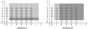
Theorem 1: Let c1,c2,μ1,μ2 > 0, p ∈ [0,1]. For c1 /c2 ∈ A, in the preemptive model it is always optimal to allocate both servers to queue 2 (if possible) (i.e.,

for i ≥ 1, j ≥ 2, and

for i ≥ 2) (see Fig. 1a).

The control matrix for regions A and B.
Theorem 2: Let c1,c2,μ1,μ2 > 0, p ∈ [0,1]. For c1 /c2 ∈ B, in the preemptive model it is always optimal to allocate both servers to queue 1 (if possible) (i.e.,

for i ≥ 2, j ≥ 1, and

for j ≥ 2) (see Fig. 1b).
In the case μ2 = μ1(1 − p), there are only pure strategies; more precisely, the following statement holds.
Corollary 1: Let c1,c2,μ1,μ2 > 0,p ∈ [0,1], and assume that μ2 = μ1(1 − p) holds; then for c1 /c2 < 1 (c1 /c2 > 1), it is always optimal to allocate both servers to queue 2 (queue 1) (if possible).
Note that the case μ2 = μ1(1 − p) and c1 = c2 is a kind of equilibrium, in which for each state (i,j) all possible controls give the same expected holding costs. Moreover, note that μ2 = μ1(1 − p) is possible if and only if p < 1.
Theorems 1 and 2 give the optimal strategy in the preemptive model. Given any strategy, the expected holding costs in each state (i,j), until the system is empty, in the preemptive model are less than or equal to those in the nonpreemptive model because of the memoryless of the exponential distribution. Therefore, if the optimal control of the preemptive model can be satisfied in the nonpreemptive one along all paths to the state (0,0), then the optimal control is the same for the nonpreemptive model. Since this is true in the cases of Theorems 1 and 2 (see Figs. 1a and 1b), we arrive at the following corollary for the nonpreemptive model.
Corollary 2: Let c1,c2,μ1,μ2 > 0, p ∈ [0,1]. For c1 /c2 ∈ A ∪ B, the optimal control in the nonpreemptive model is the same as in the preemptive model.
Remark: Now the sufficient conditions given in Theorems 1 and 2 will be explained. We will only consider the case μ2 > μ1(1 − p); the arguments for the other case are analogous.
(a) If

then, by Theorem 1, it is always optimal to allocate both servers to queue 1. Since (7) is equivalent to

these conditions can be interpreted as follows: If the LEPT (largest expected processing time) rule and the cμ rule suggest the same strategy (allocation to queue 1), then this strategy is optimal.
(b) If

then the LEPT rule and the cμ rule suggest different strategies. Thus, a somewhat “stronger” condition for c1 /c2 given by

is needed to guarantee that it is always optimal to allocate both servers to queue 2. Note that the last condition arises from comparing the two possible strategies in the state X = (1,2).
4. PROOF OF THE MAIN RESULTS
To proceed toward the proofs of our main theorems, we have to compute some costs and characterize the structure of the control matrix. The following lemma states that for every state (i,j), i,j ≥ 2, it is sufficient to consider only the two strategies X = 11 and X = 22.
Lemma 1: For i,j ≥ 2,

Proof: Let i,j ≥ 2. Then the dynamic equations (1) give

Thus, V(i,j,12) is a convex combination of V(i,j,11) and V(i,j,22), which gives (9). █
Lemma 2:
(a) For j ≥ 1,

(b) Let j ≥ 1. If

for k ∈ {1,2,…,j − 1}, then V(1,j,12) is given explicitly by

Proof: Straightforward computation using the dynamic equations (1). █
Lemma 3: Let i ≥ 1, j ≥ 2 and c1 /c2 < p + μ2 /μ1. If

, then

.
Proof: Let

; then by the dynamic equations (1) and (2),

Lemma 4: Let i ≥ 2, j ≥ 1 and c1 /c2 > p + μ2 /μ1. If

, then

.
Proof: Let

; then by the dynamic equations (1) and (2),

Lemma 5: For μ1,μ2 > 0, p ∈ [0,1], we have

Proof: By simple computation, we obtain that (12) is equivalent to

which is equivalent to

which gives the assertion. █
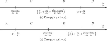
Straightforward computation gives the following lemma (see Fig. 2, in sect. 5).
Lemma 6: If μ2 > μ1(1 − p), then

if μ2 < μ1(1 − p), then

Lemma 7: For i = 1 and j = 2, we have

For c1 /c2 = (pμ1 + 2μ2)/(μ1 + μ2), we have V(1,2,12) = V(1,2,22).
Proof: By Lemma 2(b),

which gives the assertion. █
Lemma 8: For i = 2 and j = 1, we have

For

we have V(2,1,11) = V(2,1,12).
Proof: By the dynamic equations (1),

Now we distinguish between two cases.
Case 1:

By Lemma 7, V(1,2,R) = V(1,2,12); hence, by Lemma 2(b),

Case 2:

hence, by Lemma 6,

By Lemma 7, V(1,2,R) = V(1,2,22); hence, by Lemma 2(b),

which is always positive, since

and, by Lemma 5,

Lemma 9: For

.
Proof: Induction on j, j ≥ 2. Let c1 /c2 ∈ A. By (5) and Lemmas 6 and 7,

. Now, suppose that

holds; then by

we get the inequality

Further, by the induction hypothesis V(1,j,R) = V(1,j,22), we get

Thus, by (13) and Lemma 2(a),

which is negative by (5). Hence,

, which concludes the induction. █
Lemma 10: For

.
Proof: Induction on j, j ≥ 2. Let c1 /c2 ∈ B. By (6) and Lemmas 6 and 7,

. Now suppose that

, for 1 ≤ k ≤ j. Using Lemma 2(b), we get

Thus, V(1,j + 1,12) − V(1,j + 1,22) < 0 is equivalent to

We consider two cases for proving (14):
If μ2 > μ1(1 − p), then the left-hand side of (14) is negative and, since, by (6), c1 /c2 > p + (μ2 /μ1), the right-hand side of (14) is positive, which gives (14).
If μ2 < μ1(1 − p), then

where the second inequality is equivalent to

which is true by Lemma 6 and since c1 /c2 ∈ B. █
Lemma 11: For i ≥ 2, suppose that

, and define

then Bi is given explicitly by

Proof: Using the dynamic equations (2) and since

, we get

thus

By using (17) and

, we get

Proceeding analogously for V(i + 1,1,12), we get

This leads us, using definition (15), to the difference equation

which is solved by the common methods [3, §2.4]. The difference equation (18) has the characteristic roots 1 and μ1(1 − p)/(μ1 + μ2) and the special inhomogenous solution −c1(pμ1 + μ2)i/2μ1μ2. Hence, we get

where A0 and A1 have to be chosen such that the initial conditions

are satisfied. After some lengthly computation, one gets

which gives formula (16). █
Proof of Theorem 1: Let c1 /c2 ∈ A. By Lemma 9,

. Hence, by Lemmas 3 and 6, it follows that

for i ≥ 2, j ≥ 2. Thus, it remains to show that

, which is managed by induction on i. By (5) and Lemmas 6 and 8, we have

. Now suppose that

; then using Lemma 11,

Now we consider two cases. If μ2 > μ1(1 − p), then

which is positive by Lemma 5 and c1 /c2 ∈ A. If μ2 < μ1(1 − p), then

which is positive by Lemma 6 and c1 /c2 ∈ A.
Hence, the induction is finished and the theorem is entirely proved. █
Proof of Theorem 2: Let c1 /c2 ∈ B. By Lemma 10,

. We show by induction on i that

; then by Lemmas 4 and 6,

, and the theorem is proved.
By Lemma 8, we have

. Moreover,

So,

is equivalent to

Since in the case μ2 > μ1(1 − p), G < p + μ2 /μ1 and in the case μ2 < μ1(1 − p),

we have

. Now suppose that

for some i ≥ 3. Thus, by Lemmas 4 and 6,

. Since V(i,1,12) − V(i,1,11) ≥ 0, we get the inequality

Then, using inequality (19),

Since

, we have V(i − 1,3,22) ≥ V(i − 1,3,11) and V(i − 1,2,22) ≥ V(i − 1,2,11); thus, by (1 − 2p)(1 − p) = (1 − p)2 − p(1 − p), we get

Hence, the proof is finished. █
5. DISCUSSION
In [4], Pandelis and Teneketzis optimized the α-discounted holding cost problem with general service times and m servers. Translated into our situation (i.e., exponentially distributed service time, m = 2 servers and α = 0), their result reads as follows.
Theorem 3 [4]: For μ1 > μ2 and c1 /c2 ≥ 1 + p, in the nonpreemptive case it is always optimal to allocate both servers to queue 1 (if possible).
Note that if μ2 > μ1(1 − p), we have

and if μ2 > μ1(1 − p), we have

Hence, in both cases the region for a pure “11” strategy that we found is larger than that in [4], where our assumptions are more restrictive than those in [4].
Now we separate the parameter region for c1 /c2 into four regions, denoted by A, C, D, and B, as shown in Figs. 2a and 2b. For regions A and B, we have given the optimal control in Theorem 1 and Theorem 2. For regions C and D, we conjecture the following:
Conjecture 1:
(a) Let μ2 > μ1(1 − p) (see Fig. 2a).
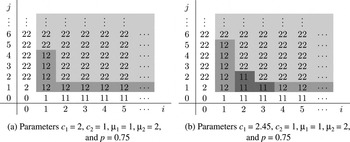
(i) For c1 /c2 ∈ C, there exists an index j* for the first column such that

if j ≤ j* and

if j > j* (see Fig. 3a, where j* = 4). Further,

.
(ii) For c1 /c2 ∈ D, the control matrix

consists of a triangular region of “11” and the rest of the control matrix is “22.” This triangular region increases, if c1 /c2 increases (see Figs. 3b and 1b).
(b) Let μ2 < μ1(1 − p) (see Fig. 2b).
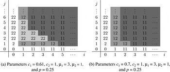
(i) For c1 /c2 ∈ D, there exists an index i* such that

if i ≤ i* and

if i > i* (see Fig. 4b, where i* = 2). Further,

.
(ii) For c1 /c2 ∈ C, there is a triangular region of “22” and the rest of the control matrix is “11,” where this triangular region increases if c1 /c2 increases (see Figs. 4a and 1a).

Parameter regions for c1 /c2 in two cases.

Control matrix in the case μ2 > μ1(1 − p).

Control matrix in the case μ2 < μ1(1 − p).
The case p = 1 has been completely solved by the authors in [6] for the preemptive case. Note that the case μ2 < μ1(1 − p) is not possible; hence, only part (a) of the above conjecture is decisive and was proved in [6]. Note that the region for a pure “22” (resp. “11”) strategy changes from c1 /c2 ≤ (μ1 + 2μ2)/(μ1 + μ2) (resp. c1 /c2 ≥ 1 + (μ2 /μ1)) in the case p = 1 to c1 /c2 ≤ (pμ1 + 2μ2)/(μ1 + μ2) (resp. c1 /c2 ≥ p + (μ2 /μ1)) in the case of general p ∈ [0,1].
For the general model with m servers, it is very hard to prove the optimal strategy. The case p = 0 has partly been solved by the authors in [7]. Furthermore, numerical examples show that the conditions (for general p) for the pure strategies are analogous to the conditions in the two-server model. Therefore, we state the following conjecture:
Conjecture 2:
(a) Assume that μ2 > μ1(1 − p); then in the m-server model, it is optimal to allocate all servers to queue 2 or queue 1 if and only if

respectively.
(b) Assume that μ2 < μ1(1 − p); then in the m-server model, it is optimal to allocate all servers to queue 2 if and only if

(c) Assume that μ2 = μ1(1 − p); then in the m-server model, it is optimal to allocate all servers to queue 2 or queue 1 if and only if

respectively.
For the sake of completeness, we state the optimal control for the one-server problem. The proof is straightforward and therefore omitted.
Theorem 4: In the case of one server, it is always optimal to serve a job of queue 1 or queue 2 (if possible) if and only if

respectively.
Note that, if c1 /c2 = p + μ2 /μ1, then in every point (i,j) of the control matrix

, we have two possible strategies, namely to take a job of queue 1 or to take a job of queue 2.
Acknowledgments
We would like to thank P. Weiß and C. Takacs for many discussions on the subject.
References
REFERENCES
Ahn, H.,
Duenyas, I., &
Zhang, R.Q.
(1999).
Optimal stochastic scheduling of a two-stage tandem queue with
parallel servers.
Advances in Applied Probability
31:
1095–1117.Google Scholar
Chang, C.S.,
Nelson, R., &
Pinedo, M.
(1991).
Scheduling two classes of exponential jobs on parallel processors:
Structural results and worst-case analysis.
Advances in Applied Probability
23:
925–944.Google Scholar
Elaydi, S.N.
(1996).
An introduction to difference equations.
New York:
Springer-Verlag.
Pandelis, D.G. &
Teneketzis, D.
(1994).
Optimal multiserver stochastic scheduling of two interconnected
priority queues.
Advances in Applied Probability
26:
258–279.Google Scholar
Ross, S.
(1983).
Introduction to stochastic dynamic programming.
New York:
Academic Press.
Schiefermayr, K. &
Weichbold, J.
(2005).
A complete solution for the optimal stochastic scheduling of a
two-stage tandem queue with two flexible servers.
Journal of Applied Probability
42:
778–796.Google Scholar
Schiefermayr, K. &
Weichbold, J.
(2006).
A scheduling problem of several parallel servers
(submitted).
The control matrix for regions A and B.
Parameter regions for c1 /c2 in two cases.
Control matrix in the case μ2 > μ1(1 − p).
Control matrix in the case μ2 < μ1(1 − p).
 You have
Access
- 5
- Cited by