2.1. TVaR and TVaR-based capital allocation

Let us recall the definition of the aggregate claim amount $S_n$ given by (1.1). The VaR at level $\kappa$ , $0 < \kappa < 1$ , of $S_n$ is defined by $\textrm{VaR}_{\kappa}(S_n)=\textrm{inf}\{x \in {\mathbb R}, F_{S_n}(x) \ge \kappa\}$ , where $F_{S_n}$ denotes the c.d.f. of $S_n$ . The TVaR at level $\kappa$ , $0 < \kappa < 1$ , of $S_n$ is defined by

(2.1) \begin{align}\textrm{TVaR}_{\kappa}(S_n)&=\frac{1}{1-\kappa}{\int_\kappa ^1 {{\textrm{Va}}{{\textrm{R}}_u}({S_n})} du} \nonumber \\&=\frac{{\textrm{E}\left[S_n \times {\mathbb 1}_{\{{S_n > \textrm{VaR}_{\kappa}(S_n)}\}}\right]}+\textrm{VaR}_{\kappa}(S_n)(F_{S_n}(\textrm{VaR}_{\kappa}(S_n))-\kappa)}{1-\kappa},\end{align}

where ${\mathbb 1}_A$ is the indicator function such that ${\mathbb 1}_A(x)=1$ if $x \in A$ , and ${\mathbb 1}_A(x)=0$ , if $x \notin A$ .

Note that the r.v. $S_{i,n}$ given by (1.2) is continuous under the assumption of continuous and strictly positive claim sizes, implying that the r.v. $S_n$ is also continuous. Then, $F_{S_n}(\textrm{VaR}_{\kappa}(S_n))-\kappa=0$ and (2.1) becomes

\begin{equation*}\textrm{TVaR}_{\kappa}(S_n)=\frac{{\textrm{E}\left[S_n \times {\mathbb 1}_{\{{S_n > \textrm{VaR}_{\kappa}(S_n)}\}}\right]}}{1-\kappa}.\end{equation*}

It is well known that the VaR is not a coherent risk measure. In this paper, we consider to determine the amount of capital for the whole portfolio with the TVaR-based rule. For $0<\kappa<1$ , the allocated capital to each risk $S_{i,n}$ under the TVaR-based allocation rule is given by

\begin{equation*}{K_i} = \frac{{\textrm{TVaR}_{\kappa}(S_{i,n};\;S_n)}}{{\textrm{TVaR}_{\kappa}(S_n)}}K,\end{equation*}

where K is a given total risk capital and

\begin{equation*}\textrm{TVaR}_{\kappa}(S_{i,n};\;S_n)=\frac{\textrm{E}\left[S_{i,n} \times {\mathbb 1}_{\{{S_n > \textrm{VaR}_{\kappa}(S_n)}\}}\right]}{1-\kappa}.\end{equation*}

It implies that the capital required for the entire portfolio is equal to the sum of the allocated capital of each risk within the portfolio, that is, $\sum\nolimits_{i=1}^{n}{K_i}=K$ . See for example McNeil et al. (Reference McNeil, Frey and Embrechts2015) for details on the risk measures VaR and TVaR, and the TVaR-based allocation rule.

This paper considers the particular case that $K={\textrm{TVaR}_{\kappa}(S_n)}$ , which coincides with the TVaR-based allocation rule suggested by Bargès et al. (Reference Bargès, Cossette and Marceau2009), Cossette et al. (Reference Cossette, Mailhot and Marceau2012, Reference Cossette, Côté, Marceau and Moutanabbir2013, Reference Cossette, Marceau and Perreault2015), and Ratovomirija et al. (Reference Ratovomirija, Tamraz and Vernic2017).

2.2. MINAR(1) processes

Let ${\textbf{N}_k}=(N_{1,k},...,N_{d,k})$ and ${\textbf{e}_k}=(e_{1,k},...,e_{d,k})$ be non-negative integer-valued random vectors. ${\textbf{N}}_k$ is independent of the i.i.d. sequence $\{\textbf{e}_k\}_{k \in \mathbb Z}$ . Let $\textbf{A}$ be a $d \times d$ matrix with independent elements $\{\alpha_{ij}\}_{i,j=1}^d$ . The multivariate INAR(1) process $\{{\textbf{N}_k}\}_{k \in \mathbb Z}$ based on the binomial thinning operation is defined by

(2.2) \begin{equation}{\textbf{N}_k} = {\textbf{A}} \circ {\textbf{N}_{k - 1}} + {\textbf{e}_k}\end{equation}

with its i-th element given by

(2.3) \begin{equation}N_{i,k}=\sum\limits_{j = 1}^d {{\alpha _{ij}} \circ {N_{j,k - 1}}} + {e_{i,k}},\;\;i=1,...,d.\end{equation}

In (2.2), the binomial thinning operators $\alpha_{ij} \circ$ are mutually independent, for $i,j=1,...,d$ . Each operator is defined by ${\alpha_{ij}} \circ N=\sum\nolimits_{k = 1}^N {{\delta _k}}$ , where $\{ {\delta _k}\} _{k = 1}^N$ is a sequence of i.i.d. Bernoulli r.v.s such that $\textrm{E}[{\delta_k}]=\alpha_{ij}$ and $\alpha_{i,j} \in [0,1)$ .

The process $\{\textbf{N}_k\}_{k \in \mathbb Z}$ satisfying (2.2) is stationary if the largest eigenvalue of the matrix $\textbf{A}$ is less than 1 and $\textrm{E} \left\| {\textbf{e}_k} \right\| < \infty $ (Pedeli and Karlis, Reference Pedeli and Karlis2013b). The process $\{{\textbf{e}}_k\}_{k \in \mathbb Z}$ entered in (2.2) is known as the innovations.

The MINAR(1) process introduced above is particularly convenient for modeling dependence structures between multivariate risks. As an example, ${\textbf{N}_k}$ may be interpreted as the number of claims in period k for an insurance portfolio with d lines of business. As every INAR-type process, ${\textbf{N}_k}$ is composed of two different parts. The first consists of proportions of the number of claims from the previous period $k-1$ , denoted by ${\textbf{N}_{k-1}}$ . The time dependence between the number of claims of a fixed line of business over time arises from this part. The second part consists of the innovations that are assumed to be dependent. The cross-dependence between the number of claims from different lines of business derives from the covariance structure assumed for ${\textbf{e}_k}$ . For further applications, we refer the readers to Pedeli and Karlis (Reference Pedeli and Karlis2013a, Reference Pedeli and Karlis2013b) and Darolles et al. (Reference Darolles, Le Fol, Lu and Sun2019).

In the literature, there are two kinds of MINAR(1) processes, depending on the form of the matrix ${\textbf{A}}$ entered in (2.2).

In Definition 2.1, from (2.3) each series separately follows a univariate INAR(1) process, thus allowing for time dependence. The assumption of diagonality implies that the correlation between innovations is the only source of cross-dependence between the series $\{N_{ik},N_{jk}\}$ , for $i,j=1,...,d$ and $i \ne j$ . Therefore, two sources of dependence are arising in the basic MINAR(1) process. Detailed properties and methods of estimation about the basic MINAR(1) process have been discussed extensively in Pedeli and Karlis (Reference Pedeli and Karlis2013a).

Compared with Definition 2.1, an extra source of dependence is incorporated into the process by relaxing the diagonality assumption of the matrix ${\textbf{A}}$ in Definition 2.2. More specifically, the value of each series in period k is directly not only to its own observations but also to the observations of the others series at the preceding point in period $k-1$ , see (2.3). This forms the third source of dependence and is referred to cross-time dependence as in Bermúdez et al. (Reference Bermúdez, Guillén and Karlis2018). Some distributional properties and methods of estimation for the full MINAR(1) process can be found in Pedeli and Karlis (Reference Pedeli and Karlis2013b).

In this paper, the sequence of innovations $\{{\textbf{e}}_k\}_{k \in \mathbb Z}$ ( ${\textbf{e}}_k \sim {\textbf{e}}$ ) in (2.2) is assumed to jointly follow a multivariate Poisson distribution, which is defined by the linear equation

(2.4) \begin{equation}{\textbf{e}}^T=(e_1,...,e_d)^T={\textbf{B}}{\underline \xi}.\end{equation}

In (2.4), ${\textbf{B}}=({\textbf{I}}_d, {\textbf{B}}^{*})$ is a $d \times \frac{d(d+1)}{2}$ matrix where ${\textbf{I}}_d$ is the identify matrix of dimension d and ${\textbf{B}}^{*}=(b_{1,2},...,b_{1,d},b_{2,3},...,b_{2,d},...,b_{d-1,d})$ is a $d \times \frac{d(d-1)}{2}$ matrix with $b_{i,j}$ being a column vector of dimension d, whose i-th and j-th elements are one and the rest are zero, for $i,j=1,...,d$ and $i<j$ . ${\underline \xi}=(\xi_1,...,\xi_d,\xi_{1,2},...,\xi_{1,d},\xi_{2,3},..,\xi_{2,d},...,\xi_{d-1,d})^T$ is a sequence of independent r.v.s, where ${\xi_i}$ and ${\xi_{i,j}}$ are Poisson distributed with mean $\lambda_i$ and $\lambda_{i,j}$ , respectively, that is, ${\xi_i} \sim \textrm{Poi}(\lambda_i)$ and $\xi_{i,j} \sim \textrm{Poi}(\lambda_{ij})$ , for $i,j=1,...,d$ and $i<j$ .

According to (2.4), it implies that the joint probability generating function (p.g.f.) of ${\textbf{e}}=(e_1,...,e_d)$ is

\begin{equation*}p_{\textbf{e}}(\textbf{z})={{p}_{{e_1},...,{e_d}}}({z_1},...,{z_d}) = \prod\limits_{i = 1}^d {{e^{{\lambda _i}({z_i} - 1)}}{e^{\sum\nolimits_{j > i} {{\lambda _{ij}}({z_i}{z_j} - 1)} }}}.\end{equation*}

Then, the stationary marginal distribution of $\{\textbf{N}_k\}_{k \in \mathbb Z}$ can be determined by the equation

(2.5) \begin{equation}{p_{\textbf{N}}}({\textbf{z}}) = {p_{{\textbf{A}} {\circ} {\textbf{N}}}({\textbf{z}}){p_{{\textbf{e}}}({\textbf{z}})}}.\end{equation}

2.3. Mixed Erlang distributions

The mixed Erlang distribution has many attractive properties when modeling the individual claim sizes of an insurance portfolio (see, e.g., Lee and Lin, Reference Lee and Lin2010 and Willmot and Lin, Reference Willmot and Lin2011). We begin this subsection with the definition of the mixed Erlang distribution and continue with some properties about it.

Let the probability density function (p.d.f.) and c.d.f. of an Erlang distribution of order k be

\begin{equation*}{h}(x;\; k, \beta) = \frac{{{\beta ^k}}}{{(k - 1)!}}{x^{k - 1}}{e^{ - \beta x}}, {\kern 5pt} x>0,\end{equation*}

and

\begin{equation*}{H}(x;\; k, \beta ) = 1 - {e^{ - \beta x}}\sum\limits_{j = 0}^{k - 1} {\frac{{{{(\beta x)}^j}}}{{j!}}}, {\kern 5pt} x>0,\end{equation*}

where $\beta>0$ and $k \in {\mathbb N}$ .

Let X be a mixed Erlang r.v. with scale parameter $\beta$ . The p.d.f. and c.d.f. of X are respectively given by

\begin{equation*}{f_X}(x) = \sum\limits_{j = 1}^\infty {{q_j}{h}(x;\; j, \beta)},\end{equation*}

and

\begin{equation*}{F_X}(x) = \sum\limits_{j = 1}^\infty {{q_j}{H}(x;\; j, \beta)},\end{equation*}

where $\underline q=\{q_j\}_{j=1}^{\infty}$ is a vector of non-negative mixing probabilities such that $\sum\nolimits_{j = 1}^\infty {{q_j}} = 1$ .

Based on the analytical form of ${F_X}(x)$ , the expression for $\textrm{TVaR}_{\kappa}(X)$ is given by

(2.6) \begin{equation}\textrm{TVaR}_{\kappa}(X)=\frac{1}{1-\kappa}{\sum\limits_{j=1}^{\infty}{{q_j}\frac{j}{\beta}\overline H({\textrm{VaR}_{\kappa}(X)};\; j+1,\beta)}},\end{equation}

where $\overline H({\textrm{VaR}_{\kappa}(X)};\; j,\beta)=1- H({\textrm{VaR}_{\kappa}(X)};\; j,\beta)$ and $\textrm{VaR}_{\kappa}(X)$ can be computed numerically from the equation ${F_X}(\textrm{VaR}_{\kappa}(X))-\kappa=0$ . Here and henceforth, we use the notation $X \sim \textrm{MixErl}(\underline q, \beta)$ with ${\underline q}=\{q_j\}_{j=1}^{\infty}$ for convenience.

The rest of this subsection provides some distributional properties of the mixed Erlang distribution, which will be convenient for us to identify that many other r.v.s can be expressed in the form of an Erlang mixture in the sequel.

Lemma 2.1. Let X be a r.v. with X ~ MixErl $(\underline q, \beta_1)$ and ${\underline q} = \{ {q_{j}}\} _{j = 1}^\infty $ . Then, it follows that for any positive constant $\beta$ such that $\beta_1 \le \beta$ , the p.d.f. of X can be expressed as the p.d.f. of a mixed Erlang distribution with parameters $(\underline \omega (\underline q, \beta_1, \beta) = \{\omega_j(\underline q, \beta_1, \beta)\}_{j=1}^{\infty}, \beta)$ , where

\begin{equation*}\omega_j({\underline q},{\beta _1},{\beta}) = \sum\limits_{k = 1}^j {{q_k}\dbinom{j-1}{j-k}{{\left( {\frac{{{\beta_1}}}{{{\beta}}}} \right)}^k}{{\left( {1 - \frac{{{\beta_1}}}{{{\beta}}}} \right)}^{j - k}}}, {\kern 5pt} j=1,2,....\end{equation*}

Assume that $X_i \sim \textrm{MixErl}(\underline q_i, \beta_i)$ with ${\underline q_i} = \{{q_{ij}}\} _{j = 1}^\infty$ for $i \in {\mathbb N}$ . By Lemma 2.1, each $X_i$ can be transformed into a new mixed Erlang distribution with a common scale parameter. Without loss of generality, it will be assumed that $\beta_i=\beta$ in the sequel.

Lemma 2.2. Let $X_1$ and $X_2$ be two independent r.v.s with $X_i \sim {\textrm {MixErl}}(\underline q_i, \beta)$ and ${\underline q_i} = \{ {q_{ij}}\} _{j = 1}^\infty $ , for $i=1,2$ . Then, the r.v. $Z_2={X_1}+{X_2}$ has a mixed Erlang distribution with parameters $(\underline \sigma(\underline q_1, \underline q_2)=\{\sigma_j(\underline q_1,\underline q_2)\}_{j=1}^{\infty}, \beta)$ , where

\begin{equation*}{\sigma}_j({\underline q_1},{\underline q_2}) = \left\{\begin{aligned}\sum\limits_{k=1}^{j-1}{q_{1,k}{q_{2,j-k}}}, & & j>1, \\ 0, & & j=1.\end{aligned} \right.\end{equation*}

2.4. Compound distributions with mixed Erlang claim sizes

Another and quite useful expression can be given to the class of mixed Erlang distributions. To do so, we first make a notation for compound distributions. Let a r.v S have a compound distribution with

\begin{equation*}S=\left\{\begin{aligned}\sum\limits_{k = 1}^N {{X_k}},& &N >0, \\0,& &N=0,\\\end{aligned} \right.\end{equation*}

where N is a discrete r.v. with p.m.f. $\Pr(N=j)=p_j$ for $j \in {\mathbb N_0}$ and ${\underline X}=\{X_k\}_{k=1}^{\infty}$ is a sequence of i.i.d. r.v.s ( $X_k \sim X$ ) and independent of N. To simplify the presentation, we denote the compound r.v. S as $S:=N \vee {\underline X}$ in what follows.

A mixed Erlang distribution X can be interpreted as a compound distribution such that X follows $X=J \vee \underline E$ , where J is a discrete r.v. with p.m.f. $\Pr(J=0)=0$ and $\Pr(J=j)=q_j$ , for $j >0 $ , and ${\underline E}=\{ {E_k}\} _{k = 1}^\infty$ is a sequence of i.i.d. r.v.s, following an exponential distribution with parameter $\beta$ , that is, $E_k \sim \textrm{Exp}(\beta)$ . This interpretation of the mixed Erlang distribution enables us to derive the expression for the TVaR of some compound distributions with mixed Erlang claim sizes, which will be examined in the following lemmas.

Lemma 2.3. Let the r.v N have a Bernoulli distribution with mean $\alpha$ , that is, $N \sim \textrm{Bern}(\alpha)$ . Suppose that ${\underline X}=\{ {X_k}\} _{k = 1}^\infty$ is a sequence of i.i.d. r.v.s with X_k ~ MixErl $(\underline q, \beta)$ and $\underline q=\{q_j\}_{j=1}^{\infty}$ . Then the c.d.f. of the compound r.v. $Y= N \vee {\underline X}$ follows

(2.7) \begin{equation}{F_Y}(x) = {p_0} + \sum\limits_{j = 1}^\infty {{p_j}H(x;\;j, \beta )},\end{equation}

where $p_0=1-\alpha$ and $p_j=\alpha q_j$ , for $j \ge 1$ .

It is clear from (2.7) that $F_Y(x)$ combines a mixed Erlang distribution on the positive real line and a point mass at zero. In what follows, we use the notation $Y \sim \textrm{MixErl}(\underline p, \beta)$ with ${\underline p}=\{p_j\}_{j=0}^{\infty}$ to represent a mixed Erlang r.v. by allowing a point mass $p_0$ at zero.

Lemma 2.4. Let $Y_1$ and $Y_2$ be two independent r.v.s with $Y_i={N_i} \vee {\underline X_i}$ , where $N_i \sim \textrm{Bern}(\alpha_i)$ and ${\underline X_i}=\{ {X_{i,k}}\} _{k = 1}^\infty$ is a sequence of i.i.d. r.v.s. with X_i,k ~ MixErl $(\underline q_i, \beta)$ and $\underline q_i=\{q_{i,j}\}_{j=1}^{\infty}$ , for $i=1,2$ . Then, the r.v. Z ₂ = Y ₁ + Y ₂ ~ MixErl $(\underline \sigma(\underline p_1, \underline p_2), \beta)$ , where $\underline \sigma(\underline p_1, \underline p_2)=\{\sigma_j(\underline p_1, \underline p_2)\}_{j=0}^{\infty}$ with

(2.8) \begin{equation}\sigma_j(\underline p_1, \underline p_2)=\sum\limits_{k=0}^{j}{p_{1,k}{p_{2,j-k}}},\end{equation}

where $\underline p_{i}=\{p_{i,j}\}_{j=0}^{\infty}$ with $p_{i,0}=1-\alpha_i$ and $p_{i,j}={\alpha_i}q_{i,j}$ , for $j \ge 1$ and $i=1,2$ .

Lemma 2.5. Let the r.v. $Y={N} \vee {\underline X}$ , where $N \sim \textrm{Poi}(\lambda)$ and ${\underline X}=\{ {X_{k}}\} _{k = 1}^\infty$ is a sequence of i.i.d. r.v.s with $X_{k} \sim \textrm{MixErl}(\underline q, \beta)$ and $\underline q=\{q_{j}\}_{j=1}^{\infty}$ . Then the c.d.f. of the compound r.v. Y is given by

\begin{equation*}{F_Y}(x) = {f_{N'}(0)} + \sum\limits_{k = 1}^\infty {{f_{N'}(k)}H(x;\; k, \beta )},\end{equation*}

where $f_{N'}$ represents the probability mass function (p.m.f.) of a non-negative integer-valued r.v. N^′, which is determined by the following recursive formula:

\begin{equation*}f_{N'}(k+1)=\frac{\lambda}{k+1}\big( {q_1}f_{N'}(k)+ 2{q_2}f_{N'}(k-1)+\cdots+(k+1){q_{k+1}f_{N'}(0)}\big),\end{equation*}

for $k \in {\mathbb N}_0$ and $f_{N'}(0)=e^{-\lambda}$ .

3.1. Joint LST of (S _1,n, …, S _d,n)

Proposition 3.1. Assuming that the number of claims $\{N_{1,k},...,N_{d,k}\}_{k \in \mathbb N}$ follow a basic MINAR(1) process, the joint LST of $(S_{1,n},...,S_{d,n})$ is given by

(3.2) \begin{align}\mathcal{L}_{S_{1,n},...,S_{d,n}}(z_1,...,z_d)=& \;{p_{{N_{1,1}},...,{N_{d,1}}}}( {G_{1,n}({\mathcal{L}_{{X_1}}}({z_1})),...,G_{d,n}({\mathcal{L}_{{X_d}}}({z_d}))} ) \nonumber \\&\!\!\times\! \prod\limits_{k = 2}^n\! {{p_{{e_{1,k}},...,{e_{d,k}}}}} (G_{1,n - k + 1}({\mathcal{L}_{\!{X_1}}}({z_1})),...,G_{d,n - k + 1}({\mathcal{L}_{\!{X_d}}}({z_d}))),\end{align}

where

(3.3) \begin{equation}G_{i,m}({z_i}) =\left\{\begin{aligned}{\left( {{\alpha_{ii}}G_{i,m - 1}({z_i}) + 1 - {a_{ii}}} \right)z_i}, && m>1, \\[5pt] z_i, && m=1,\end{aligned}\right.\end{equation}

for $i=1,...,d$ and $m=1,...,n$ .

Remark 3.1. From (3.3), $G_{i,m}(\mathcal{L}_{X_i}(z_i))$ just corresponds to the LST of a r.v. associated with $X_i$ , for $i=1,...,d$ and $m=1,...,n$ . Without loss of generality, suppose that $\{X'_{\!i,m}\}_{m=1}^{n}$ is a sequence of independent r.v.s such that the LST of $X'_{\!i,m}$ follows

(3.4) \begin{equation}\mathcal{L}_{X'_{\!i,m}}(z)=G_{i,m}(\mathcal{L}_{X_i}(z)).\end{equation}

By letting $z_1=\cdots=z_d=z$ in (3.2), the form of $\mathcal{L}_{S_{1,n},...,S_{d,n}}(z,...,z)$ indicates that the r.v. $S_n=\sum\nolimits_{i=1}^{d}{S_{i,n}}$ can be viewed as a sum of n independent compound r.v.s.

Under the assumption of multivariate Poisson innovations, combining with (3.1), it follows that $S_n$ has a compound Poisson distribution, which can be expressed as

(3.5) \begin{equation}{S_n}={M_n} \vee {\underline D^{(n)}},\end{equation}

where $M_{n} \sim \textrm{Poi}(\lambda_{S_{n}})$ with

(3.6) \begin{equation}{\lambda _{{S_n}}} =\sum\limits_{i = 1}^d {\left({{ \lambda '}_{\!\!i}} + \sum\limits_{j > i} {{{\lambda'}_{\!\!ij}}} \right)} + (n - 1)\sum\limits_{i = 1}^d {\left({\lambda _i} + \sum\limits_{j > i} {{\lambda _{ij}}} \right)}\end{equation}

and $\underline D^{(n)}=\{D_{j}^{(n)}\}_{j=1}^{\infty}$ is a sequence of i.i.d. r.v.s ( $D_{j}^{(n)} \sim D^{(n)}$ ) with common c.d.f.

(3.7) \begin{align}{F_{{D^{(n)}}}}(x) =& \sum\limits_{i = 1}^d {\left(\frac{{{{\lambda '}_{\!\!i}}}}{{{\lambda _{{S_n}}}}}{F_{{{X'}_{\!\!i,n}}}}(x) + \frac{{\sum\nolimits_{j > i} {{{\lambda'}_{\!\!ij}}} }}{{{\lambda _{{S_n}}}}}{F_{{{X'}_{\!\!i,n}} + {X'_{\!\!j,n}}}}(x)\right)} \nonumber \\[9pt] &+ \sum\limits_{i = 1}^d {\left(\frac{{{\lambda _i}}}{{{\lambda _{{S_n}}}}} {\sum\limits_{k = 2}^n }{F_{{{{{{X'}_{\!\!i,n - k + 1}}} }}}}(x) + \frac{{\sum\nolimits_{j > i} {{\lambda _{ij}}} }}{{{\lambda _{{S_n}}}}}{\sum\limits_{k = 2}^n }{F_{{{{{{X'}_{\!\!i,n - k + 1}} + {{X'}_{\!\!j,n - k + 1}}} }}}}(x)\right)}.\end{align}

Proposition 3.2. Assuming that the number of claims $\{N_{1,k},...,N_{d,k}\}_{k \in \mathbb N}$ follow a basic MINAR(1) process with multivariate Poisson innovations given by (2.4), the expression for $\textrm{TVaR}_{\kappa}(S_n)$ is

\begin{equation*}\textrm{TVaR}_{\kappa}(S_n)=\frac{\sum\limits_{k = 1}^\infty {{f_{{M_n}}}(k)\textrm{E}\Big[ {\sum\nolimits_{j = 1}^k {D_j^{(n)}} \times {{\mathbb 1}_{\sum\nolimits_{j = 1}^k {D_j^{(n)}} > {\textrm{VaR}_\kappa }({S_n})}}} \Big]} }{1-\kappa},\end{equation*}

where ${f_{{M_n}}}$ represents the p.m.f. of $M_n$ .

3.2. TVaR-based capital allocation

By letting $z_i=z$ and $z_1=\cdots=z_{i-1}=z_{i+1}=\cdots=z_d=0$ in (3.2), it follows that the r.v. $S_{i,n}$ can be expressed as

(3.8) \begin{equation}{S_{i,n}}={M_{i,n}} \vee {\underline D^{(i,n)}},\end{equation}

where $M_{i,n} \sim \textrm{Poi}(\lambda_{S_{i,n}})$ with

\begin{equation*}\lambda_{S_{i,n}}={\lambda '_{\!\!i}} + \sum\limits_{j < i} {{\lambda '_{\!\!ji}}} + \sum\limits_{j > i} {{\lambda'_{\!\!ij}}}+(n-1)\left({\lambda _i} + \sum\limits_{j < i} {{\lambda _{ji}}} + \sum\limits_{j > i} {{\lambda _{ij}}}\right)\end{equation*}

and $\underline D^{(i,n)}=\{D_{j}^{(i,n)}\}_{j=1}^{\infty}$ is a sequence of i.i.d. r.v.s ( $D_{j}^{(i,n)} \sim D^{(i,n)}$ ) with common c.d.f.

(3.9) \begin{align}{F_{{D^{(i,n)}}}}(x) & = \frac{{\lambda'_{\!\!i}} + \sum\nolimits_{j < i} {{\lambda '_{\!\!ji}}} + \sum\nolimits_{j > i} {{\lambda'_{\!\!ij}}}}{{{\lambda _{{S_{i,n}}}}}}{F_{{{X'}_{\!\!i,n}}}}(x) \nonumber \\[5pt] & \quad + \frac{{{\lambda _i} + \sum\nolimits_{j < i} {{\lambda _{ji}}} + \sum\nolimits_{j > i} {{\lambda _{ij}}}}}{{{\lambda _{{S_{i,n}}}}}}{\sum\limits_{k = 2}^n }{F_{{{{{X'}_{\!\!i,n - k + 1}}}}}}(x).\end{align}

By letting $z_1=\cdots=z_{i-1}=z_{i+1}=\cdots=z_d=z$ and $z_i=0$ in (3.2), it follows that the r.v. $S_{-i,n}=\sum\nolimits_{l = 1,l \ne i}^d {{S_{l,n}}}$ has a compound Poisson distribution, which can be further expressed as a sum of two independent items, that is,

(3.10) \begin{equation}{S_{-i,n}}={J_{-i,n}} \vee {\underline D^{(-i,n)}} + {J_{n}^{(i)}} \vee {\underline C^{(-i,n)}}.\end{equation}

where $J_{-i,n} \sim \textrm{Poi}(\lambda_{J_{-i,n}})$ and $J_{n}^{(i)} \sim \textrm{Poi}(\lambda_{J_n^{(i)}})$ with

\begin{equation*}\lambda_{J_{-i,n}} =\sum\limits_{l = 1,l \ne i}^d {{{\lambda'}_{\!\!l}}} + \sum\limits_{l = 1,l \ne i}^d {\sum\limits_{j > l,j \ne i} {{{\lambda'}_{\!\!lj}}} } + (n - 1)\left(\sum\limits_{l = 1,l \ne i}^d {{\lambda _l}} + \sum\limits_{l = 1,l \ne i}^d {\sum\limits_{j > l,j \ne i} {{\lambda _{lj}}} } \right)\end{equation*}

and

\begin{equation*}\lambda_{J_{n}^{(i)}} =\sum\limits_{l < i} {{{\lambda'}_{\!\!li}}} + \sum\limits_{l > i} {{{\lambda}_{il},}} + (n - 1)\left(\sum\limits_{l < i} {{\lambda _{li}}} + \sum\limits_{l > i} {{\lambda _{il}}} \right),\end{equation*}

$\underline D^{(-i,n)}=\{D_{j}^{(-i,n)}\}_{j=1}^{\infty}$ and $\underline C^{(-i,n)}=\{C_{j}^{(-i,n)}\}_{j=1}^{\infty}$ are two independent sequences of i.i.d. r.v.s ( $D_{j}^{(-i,n)} \sim D^{(-i,n)}$ , $C_{j}^{(-i,n)} \sim C^{(-i,n)}$ ), independent of $\underline D^{(i,n)}$ with common c.d.f.s

(3.11) \begin{align}{F_{{D^{(-i,n)}}}}(x) &= \sum\limits_{l \ne i} {\frac{{{{\lambda'}_{\!\!l}}}}{{{\lambda _{{J_{-i,n}}}}}}{F_{{{X'}_{\!\!l,n}}}}(x)} +\sum\limits_{l \ne i} {\sum\limits_{j > l,j \ne i} {\frac{{{{\lambda'}_{\!\!lj}}}}{{{\lambda _{{J_{-i,n}}}}}}} } {F_{{{X'}_{\!\!l,n}} + {{X'}_{\!\!j,n}}}(x)} \nonumber \\[5pt] & \quad + \sum\limits_{l \ne i} {\frac{{ {\lambda _{l}}}}{{{\lambda _{{J_{-i,n}}}}}}\sum\limits_{k = 2}^n {{F_{{{X'}_{\!\!l,n - k + 1}}}(x)}} } \nonumber \\[5pt] & \quad + \sum\limits_{l \ne i} {\sum\limits_{j > l,j \ne i} {\frac{{{{\lambda}_{lj}}}}{{{\lambda _{{J_{-i,n}}}}}}} } \sum\limits_{k = 2}^n {{F_{{{X'}_{\!\!l,n - k + 1}+{X'}_{\!\!j,n - k + 1}}}(x)}}\end{align}

and

(3.12) \begin{align}{F_{{C^{(-i,n)}}}}(x) = &\sum\limits_{l < i} {\frac{{{{\lambda'}_{\!\!li}}}}{{{\lambda _{{J_{n}^{(i)}}}}}}{F_{{{X'}_{\!\!l,n}}}}(x)} + \sum\limits_{l > i} {\frac{{{{\lambda'}_{\!\!il}}}}{{{\lambda _{{J_{n}^{(i)}}}}}}{F_{{{X'}_{\!\!l,n}}}}(x)} \nonumber \\[5pt] &+ \sum\limits_{l < i} {\frac{{ {\lambda _{li}}}}{{{\lambda _{{J_{n}^{(i)}}}}}}\sum\limits_{k = 2}^n {{F_{{{X'}_{\!\!l,n - k + 1}}}(x)}} } + \sum\limits_{l > i} {\frac{{{\lambda _{il}}}}{{{\lambda _{{J_{n}^{(i)}}}}}}\sum\limits_{k = 2}^n {{F_{{{X'}_{\!\!l,n - k + 1}}}}(x)} }.\end{align}

We define the pair of r.v.s $(M_{i,n},M_{-i,n})$ , whose components are given by $M_{i,n}=J_{i,n}+{J_n^{(i)}}$ and $M_{-i,n}=J_{-i,n}+{J_n^{(i)}}$ , where $J_{-i,n}$ , ${J_n^{(i)}}$ and $J_{i,n}$ are independent with $J_{i,n} \sim \textrm{Poi}(\lambda_{S_{i,n}}-\lambda_{J_n^{(i)}})$ . The joint p.m.f. of $(M_{i,n}, M_{-i,n})$ is

(3.13) \begin{equation}{f_{{M_{i,n}},{M_{-i,n}}}}({k_i},{k_{-i}}) = \sum\limits_{k = 0}^{\min\!({k_{i}},{k_{-i}})} {{f_{{J_{i,n}}}}({k_{i}} - k){f_{{J_{-i,n}}}}({k_{-i}} - k){f_{{J_n^{(i)}}}}(k)},\end{equation}

for ${k_i}, {k_{-i}} \in {\mathbb N_0}$ and $i=1,...,d$ , where $f_{J_{i,n}}$ , $f_{J_{-i,n}}$ and $f_{J_n^{(i)}}$ represent the p.m.f.s of $J_{i,n}$ , ${J_{-i,n}}$ and $J_n^{(i)}$ , respectively.

Then, we have all the elements to derive the explicit expression for $\textrm{TVaR}_{\kappa}(S_{i,n};\; S_n)$ .

Proposition 3.3. Assuming that the number of claims $\{N_{1,k},...,N_{d,k}\}_{k \in \mathbb N}$ follow a basic MINAR(1) process with multivariate Poisson innovations given by (2.4), the expression for $\textrm{TVaR}_{\kappa}(S_{i,n};\; S_n)$ is

\begin{equation*}\textrm{TVaR}_{\kappa}(S_{i,n};\; S_n)= \frac{{\sum\limits_{{k_i} = 1}^\infty {\sum\limits_{{k_{ - i}} = 0}^\infty {\sum\limits_{k = 0}^{\min\!({k_i},{k_{ - i}})} {{f_{{J_{i,n}}}}({k_i} - k){f_{{J_{ - i,n}}}}({k_{ - i}} - k){f_{{J_n^{(i)}}}}(k){\Delta _{{k_i},{k_{ - i}},k}}} } } }}{{1 - \kappa }},\end{equation*}

where, for $i=1,...,d$ ,

\begin{equation*}{\Delta_{{k_i},{k_{ - i}},k}} = E \left[ {\left( {\sum\limits_{j_1 = 1}^{{k_i}} {D_{j_1}^{(i,n)}} } \right) \times {{\mathbb 1}_{\sum\nolimits_{{j_1} = 1}^{{k_i}} {D_{{j_1}}^{(i,n)}} + \sum\nolimits_{{j_2} = 1}^{{k_{ - i}} - k} {D_{{j_2}}^{( - i,n)}} + \sum\nolimits_{{j_3} = 1}^k {C_{{j_3}}^{( -i,n)}} > {\textrm{TVaR}_\kappa}({S_n})}}} \right].\end{equation*}

3.3. Mixed Erlang claim sizes

Assume that $X_i \sim \textrm{MixErl}(\underline q_i, \beta)$ with $\underline q_i=\{q_{i,j}\}_{j=1}^{\infty}$ , for $i=1,...,d$ . From Lemmas 2.3 and 2.4, the form of ${\mathcal{L}_{{{X'}_{\!\!i,m}}}}$ given by (3.4) just corresponds to the LST of a mixed Erlang r.v., that is, ${X'_{\!i,m}} \sim \textrm{MixErl} (\underline p^{(i,m)}, \beta)$ with $\underline p^{(i,m)}= \{p_j^{(i,m)}\} _{j = 1}^\infty$ , where

(3.14) \begin{equation}p_{j}^{(i,m)}=\left\{\begin{aligned}\sum\limits_{k=0}^{j-1}{p_k^{(\alpha_{ii};\; i,m-1)}q_{i,j-k}}, && m>1, \\q_{i,j}, && m=1,\end{aligned} \right.\end{equation}

with ${p_0^{(\alpha_{ii};\; i,m)}}=1-\alpha_{ii}$ and ${p_j^{(\alpha_{ii};i,m)}}={\alpha_{ii}}{p_j^{(i,m)}}$ , for $j \in {\mathbb N}$ , $i=1,...,d$ and $m=1,...,n$ .

Then, from Lemma 2.2, the independent sum ${ X'_{\!\!i,m}}+{X'_{\!\!j,m}}$ has a mixed Erlang distribution, that is, ${ X'_{\!i,m}}+{X'_{\!\!j,m}} \sim \textrm{MixErl}(\underline \sigma({\underline p^{(i,m)}}, {\underline p^{(j,m)}}), \beta)$ with ${\underline \sigma}({\underline p^{(i,m)}}, {\underline p^{(j,m)}})=\{{\sigma}_l({\underline p^{(i,m)}, \underline p^{(j,m)}})\}_{l=1}^{\infty}$ , where

(3.15) \begin{equation}\sigma_l(\underline p^{(i,m)}, \underline p^{(j,m)})=\left\{\begin{aligned} \sum\limits_{k=1}^{l-1}{p_k^{(i,m)}p_{l-k}^{(j,m)}}, & & l>1, \\ 0, & & l=1,\end{aligned} \right.\end{equation}

for $m=1,...,n$ , $i,j=1,...,d$ and $i \ne j$ .

Therefore, we can identify that the r.v. $D^{(n)}$ with c.d.f. given by (3.7) has a mixed Erlang distribution, that is, $D^{(n)} \sim \textrm{MixErl} (\underline d^{(n)}, \beta)$ with 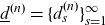$\underline d^{(n)}=\{d_s^{(n)}\}_{s=1}^{\infty}$ , where, from (3.14) and (3.15),

\begin{align*}d_s^{(n)}=&\sum\limits_{i = 1}^d {\left( {\frac{{{{\lambda'}_{\!\!i}}}}{{{\lambda _{{S_n}}}}}p_s^{(i,n)} + \frac{{\sum\nolimits_{j > i} {{{\lambda'}_{\!\!ij}}} }}{{{\lambda _{{S_n}}}}}{\sigma _s}({\underline p^{(i,n)}},{\underline p^{(j,n)}})} \right)} \\[5pt] &+ \sum\limits_{i = 1}^d {\left( {\frac{{{\lambda _i}}}{{{\lambda _{{S_n}}}}}\sum\limits_{k = 2}^n {p_s^{(i,n - k + 1)}} + \frac{{\sum\nolimits_{j > i} {{{\lambda}_{ij}}} }}{{{\lambda _{{S_n}}}}}\sum\limits_{k = 2}^n {{\sigma _s}({\underline p^{(i,n - k + 1)}},{\underline p^{(j,n - k + 1)}})} } \right)}.\end{align*}

According to Lemma 2.5 and Proposition 3.5, it follows that

\begin{equation*}\textrm{TVaR}_{\kappa}(S_n)=\frac{\sum\limits_{k=1}^{\infty}{f_{M'_{\!\!n}}(k)}\displaystyle\frac{k}{\beta}{\overline H(\textrm{VaR}_{\kappa}(S_n);\;k+1,\beta)}}{1-\kappa},\end{equation*}

where $f_{M'_{\!\!n}}$ represents the p.m.f. of a non-negative integer-valued r.v. $M'_{\!\!n}$ , which is determined by the recursive formula

\begin{equation*}{f_{{{M'}_{\!\!n}}}}(k + 1) = \frac{{{\lambda _{{S_n}}}}}{{k + 1}}\big(d_1^{(n)}{f_{{{M'}_{\!\!n}}}}(k) + 2d_2^{(n)}{f_{{{M'}_{\!\!n}}}}(k - 1) + \cdots + (k + 1)d_{k + 1}^{(n)}{f_{{{M'}_{\!\!n}}}}(0)\big),\end{equation*}

for $k \in {\mathbb N_0}$ with ${f_{{{M'}_{\!\!n}}}}(0) = {e^{ - {\lambda _{{S_n}}}}}$ and the parameter $\lambda_{S_n}$ is given by (3.6).

Also, we get that the r.v.s $D^{(i,n)}$ , $D^{(-i,n),}$ and $C^{(-i,n)}$ with c.d.f.s given by (3.9), (3.11), and (3.12) have a mixed Erlang distribution, for $i=1,...,d$ , that is, $ D^{(i,n)} \sim \textrm{MixErl} (\underline d^{(i,n)}, \beta)$ , $D^{(-i,n)} \sim \textrm{MixErl} (\underline d^{(-i,n)}, \beta),$ and $C^{(-i,n)} \sim \textrm{MixErl} (\underline c^{(-i,n)}, \beta)$ with $\underline d^{(i,n)}=\{d_s^{(i,n)}\}_{s=1}^{\infty}$ , $\underline d^{(-i,n)}=\{d_s^{(-i,n)}\}_{s=1}^{\infty}$ and $\underline c^{(-i,n)}=\{c_s^{(-i,n)}\}_{s=1}^{\infty}$ , where from (3.14) and (3.15),

\begin{equation*}d_s^{(i,n)}=\frac{{\lambda '_{\!\!i}} + \sum\nolimits_{j < i} {{\lambda '_{\!\!ji}}} + \sum\nolimits_{j > i} {{\lambda'_{\!\!ij}}}}{{{\lambda _{{S_{i,n}}}}}}{p_s^{(i,n)}} + \frac{{{\lambda _i} + \sum\nolimits_{j < i} {{\lambda _{ji}}} + \sum\nolimits_{j > i} {{\lambda _{ij}}}}}{{{\lambda _{{S_{i,n}}}}}}{\sum\limits_{k = 2}^n }{p_s^{(i,n-k+1)}},\end{equation*}

\begin{align*}{{d_s^{(-i,n)}}}= &\sum\limits_{l \ne i} {\frac{{{{\lambda'}_{\!\!l}}}}{{{\lambda _{{J_{-i,n}}}}}}{p_s^{(l,n)}} }+\sum\limits_{l \ne i} {\sum\limits_{j > l,j \ne i} {\frac{{{{\lambda'}_{\!\!lj}}}}{{{\lambda _{{J_{-i,n}}}}}}} } {{{\sigma _s}({\underline p^{(l,n)}},{\underline p^{(j,n)}})}} \\& + \!\sum\limits_{l \ne i} {\frac{{ {\lambda _{l}}}}{{{\lambda _{{J_{-i,n}}}}}}\sum\limits_{k = 2}^n {p_s^{(l,n-k+1)}} }+ \!\sum\limits_{l \ne i} {\sum\limits_{j > l,j \ne i} {\frac{{{{\lambda}_{lj}}}}{{{\lambda _{{J_{-i,n}}}}}}} } \sum\limits_{k = 2}^n {{{\sigma _s}\!\left({\underline p^{(l,n - k + 1)}},{\underline p^{(j,n - k + 1)}}\!\right)}}\end{align*}

and

\begin{align*}{{{c_s^{(-i,n)}}}} & = \sum\limits_{l < i} {\frac{{\lambda'}_{\!\!li}}{\lambda _{{J_{n}^{(i)}}}}{p_s^{(l,n)}}} + \sum\limits_{l > i} {\frac{{\lambda'}_{\!\!il}}{{\lambda _{{J_{n}^{(i)}}}}}{p_s^{(l,n)}}}\\ & \quad + \sum\limits_{l < i} {\frac{{ {\lambda _{li}}}}{{{\lambda _{{J_{n}^{(i)}}}}}}\sum\limits_{k = 2}^n {p_s^{(l,n-k+1)}}} + \sum\limits_{l > i} {\frac{{{\lambda _{il}}}}{{{\lambda _{{J_{n}^{(i)}}}}}}\sum\limits_{k = 2}^n {{p_s^{(l,n-k+1)}} }}.\end{align*}

According to Proposition 3.6, it follows that

\begin{equation*}\textrm{TVaR}_{\kappa}(S_{i,n};\; S_n)= \frac{{\sum\limits_{{k_i} = 1}^\infty {\sum\limits_{{k_{ - i}} = 0}^\infty {\sum\limits_{k = 0}^{\min ({k_i},{k_{ - i}})} {{f_{{J_{i,n}}}}({k_i} - k){f_{{J_{ - i,n}}}}({k_{ - i}} - k){f_{{J_n^{(i)}}}}(k){\Omega_{{k_i},{k_{ - i}},k}}} } } }}{{1 - \kappa }},\end{equation*}

where, for $i=1,...,d$ ,

\begin{equation*}{\Omega _{{k_i},{k_{-i}},k}} = \sum\limits_{j = 1}^\infty {\sum\limits_{l = 1}^{j-1} {d_l^{(i,n)*{k_i}}{\sigma _{j - l}}({\underline d^{(-i,n)*({k_{-i}} - k)}},{\underline c^{( - i,n)*k}})\frac{l}{\beta }{\overline H}(\textrm{{VaR}}_{\kappa}({S_n});\; j + 1,\beta )}}\end{equation*}

with

\begin{equation*}{\sigma _j}({\underline d^{( - i,n)*({k_{ - i}} - k)}},{\underline c^{( - i,n)*k}})=\left\{\begin{aligned}\sum\limits_{s = 1}^{j - 1} {d_s^{( - i,n)*({k_{ - i}} - k)}c_{j - s}^{( - i, n)*k}}, & & j>1, \\ 0, & & j=1.\end{aligned} \right.\end{equation*}

3.4. Numerical illustration

In this subsection, we consider an insurance portfolio consisting of three lines of business with $n =5$ periods. We provide two examples to numerically illustrate the impact of time and cross-dependence on the closed-form expressions for $\textrm{VaR}_{\kappa}(S_5)$ , $\textrm{TVaR}_{\kappa}(S_5),$ and $\textrm{TVaR}_{\kappa}(S_{i,5};\; S_5)$ , for $i=1,2,3$ .

The individual claim sizes are assumed to follow a mixed Erlang distribution, where ${X_i} \sim \textrm{MixErl}(\underline q_i, \beta)$ with ${\underline q_i} = \{ {q_{ij}}\} _{j = 1}^\infty $ , for $i=1,2,3$ . We set $\underline q_1=(0.2,0.3,0.5)$ , $\underline q_2=(0.3,0.4,0.3)$ , $\underline q_3=(0.5,0.1,0.4),$ and $\beta=1$ . The number of claims $\{N_{1,k},...,N_{d,k}\}_{k \in \mathbb N}$ are assumed to follow a basic MINAR(1) process with multivariate Poisson innovations given by (2.4).

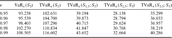
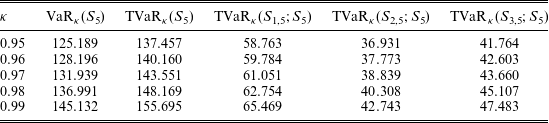
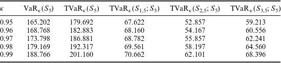
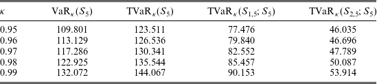
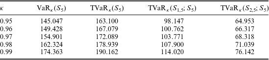
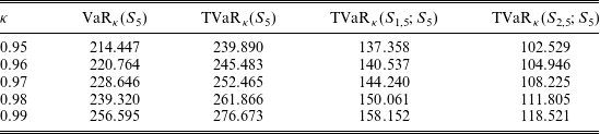
Example 3.4. Let the parameters $(\lambda_1,\lambda_2,\lambda_3)=(1,0.8,1.2)$ . Tables 1–3 display the values of $\textrm{VaR}_{\kappa}(S_5)$ , $\textrm{TVaR}_{\kappa}(S_5),$ and $\textrm{TVaR}_{\kappa}(S_{i,5};\; S_5)$ , for $\kappa=0.95,0.96,0.97,0.98,0.99$ and $i=1,2,3$ , with different time dependence parameters $\underline \alpha=(\alpha_{11},\alpha_{22}, \alpha_{33})$ and cross-dependence parameters $\underline \lambda=(\lambda_{12},\lambda_{13},\lambda_{23})$ . For the purpose of comparison, we set $\underline \alpha=(0.25, 0.2, 0.15)$ and $\underline \lambda=(0.2, 0.4, 0.3)$ in Table 1, $\underline \alpha=(0.5, 0.4, 0.3)$ and $\underline \lambda=(0.2, 0.4, 0.3)$ in Table 2, and $\underline \alpha=(0.5, 0.4, 0.3)$ and $\underline \lambda=(0.4, 0.8, 0.6)$ in Table 3.

Table 1.

Values of $\textrm{VaR}_{\kappa}(S_5)$ , $\textrm{TVaR}_{\kappa}(S_5),$ and $\textrm{TVaR}_{\kappa}(S_{i,5};\; S_5)$ ( $i=1,2,3$ ) with $\underline \alpha=(0.25, 0.2, 0.15)$ and $\underline \lambda=(0.2, 0.4, 0.3).$

Table 2.

Values of $\textrm{VaR}_{\kappa}(S_5)$ , $\textrm{TVaR}_{\kappa}(S_5),$ and $\textrm{TVaR}_{\kappa}(S_{i,5};\; S_5)$ ( $i=1,2,3$ ) with $\underline \alpha=(0.5, 0.4, 0.3)$ and $\underline \lambda=(0.2, 0.4, 0.3).$

Table 3.

Values of $\textrm{VaR}_{\kappa}(S_5)$ , $\textrm{TVaR}_{\kappa}(S_5),$ and $\textrm{TVaR}_{\kappa}(S_{i,5};\; S_5)$ ( $i=1,2,3$ ) with $\underline \alpha=(0.5, 0.4, 0.3)$ and $\underline \lambda=(0.4, 0.8, 0.6).$

From Tables 1–2, we can observe that the values of $\textrm{VaR}_{\kappa}(S_5)$ , $\textrm{TVaR}_{\kappa}(S_5),$ and $\textrm{TVaR}_{\kappa}(S_{i,5};\; S_5)$ ( $i=1,2,3$ ) increase with the time dependence level. Similarly, these values increase when the cross-dependence level increases with a comparison between Tables 2 and 3.

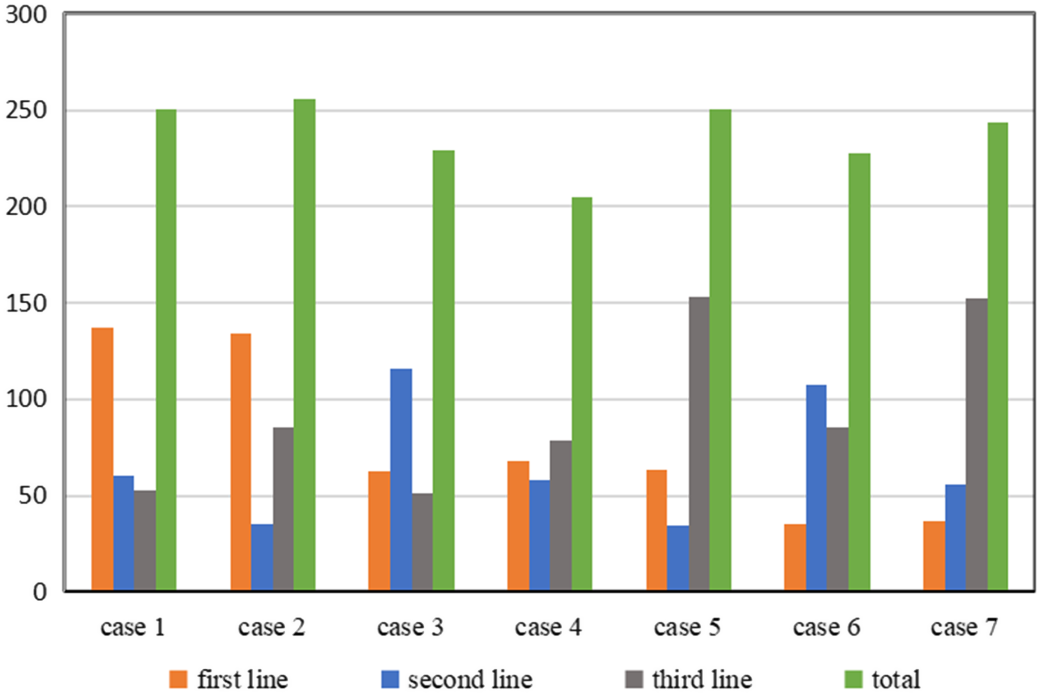
Example 3.5. Let the parameters $(\lambda_1,\lambda_2,\lambda_3)=(1,0.8,1.2)$ . In Figure 1, the cross-dependence parameters $\underline \lambda=(\lambda_{12},\lambda_{13},\lambda_{23})$ are fixed to be $(0.2, 0.4, 0.3)$ . We calculate the contribution $\textrm{TVaR}_{0.99}(S_{i,5};\; S_5)$ for the i-th line of business ( $i=1,2,3$ ) and the total of them with different time dependence parameters $\underline \alpha=(\alpha_{11},\alpha_{22}, \alpha_{33})$ . 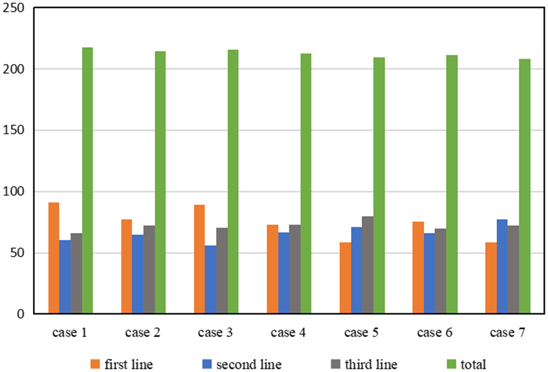We consider the following seven cases: $\underline \alpha=(0.75, 0.5, 0.25)$ for case 1, $\underline \alpha=(0.75, 0.25, 0.5)$ for case 2, $\underline \alpha=(0.5, 0.75, 0.25)$ for case 3, $\underline \alpha=(0.5, 0.5, 0.5)$ for case 4, $\underline \alpha=(0.5, 0.25, 0.75)$ for case 5, $\underline \alpha=(0.25, 0.75, 0.5)$ for case 6, and $\underline \alpha=(0.25, 0.5, 0.75)$ for case 7.

Figure 1.

Values of $\textrm{TVaR}_{0.99}(S_{i,5};\; S_5)$ ( $i=1,2,3$ ) and $\textrm{TVaR}_{0.99}(S_5)$ with different $\underline \alpha=(\alpha_{11},\alpha_{22}, \alpha_{33}).$

Similarly, the time dependence parameters $\underline \alpha=(\alpha_{11},\alpha_{22}, \alpha_{33})$ are fixed to be $(0.5, 0.4, 0.3)$ in Figure 2. The values of $\textrm{TVaR}_{0.99}(S_{i,5};\; S_5)$ ( $i=1,2,3$ ) and the total of them are presented with different cross-dependence parameters $\underline \lambda=(\lambda_{12},\lambda_{13},\lambda_{23})$ . We also consider seven cases with $\underline \lambda=(0.75, 0.5, 0.25)$ for case 1, $\underline \lambda=(0.75, 0.25, 0.5)$ for case 2, $\underline \lambda=(0.5, 0.75, 0.25)$ for case 3, $\underline \lambda=(0.5, 0.5, 0.5)$ for case 4, $\underline \lambda=(0.5, 0.25, 0.75)$ for case 5, $\underline \lambda=(0.25, 0.75, 0.5)$ for case 6, and $\underline \lambda=(0.25, 0.5, 0.75)$ for case 7.

Figure 2.

Values of $\textrm{TVaR}_{0.99}(S_{i,5};\; S_5)$ ( $i=1,2,3$ ) and $\textrm{TVaR}_{0.99}(S_5)$ with different $\underline \lambda=(\lambda_{12},\lambda_{13},\lambda_{23}).$

In Figure 1, although the mean of the time dependence parameters is equal to 0.5 for each case, the allocation for i-th line of business ( $i=1,2,3$ ), and the total of them show a different behavior. This reveals that both the parameters $(\alpha_{11}, \alpha_{22}, \alpha_{33})$ have effect on the contribution of a certain line of business. For example, letting $\alpha_{11}=0.75$ in the first two cases, the values of $\textrm{TVaR}_{0.99}(S_{1,5};\; S_5)$ are equal to $136.933$ with $(\alpha_{22}, \alpha_{33})=(0.5,0.25)$ and to $134.329$ with $(\alpha_{22}, \alpha_{33})=(0.25,0.5)$ , respectively. A similar pattern can be observed from Figure 2.

4.1. Joint LST of (S _1,n, S _2,n)

Proposition 4.1. Assuming that the number of claims $\{N_{1,k} ,N_{2,k}\}_{k \in \mathbb N}$ follow a full BINAR(1) process, the joint LST of $(S_{1,n}, S_{2,n})$ is given by

(4.2) \begin{align}\mathcal{L}_{S_{1,n},S_{2,n}}(z_1,z_2) &= {p_{{N_{1,1}},{N_{2,1}}}}\left( {G_{1,n}({\mathcal{L}_{{X_1}}}({z_1}),{\mathcal{L}_{{X_2}}}({z_2})),G_{2,n}({\mathcal{L}_{{X_1}}}({z_1}),{\mathcal{L}_{{X_2}}}({z_2}))} \right) \nonumber \\& \quad \times \prod\limits_{k = 2}^n {p_{{e_{1, k}},{e_{2,k}}}}(G_{1,n - k + 1}({\mathcal{L}_{{X_1}}}({z_1}),{\mathcal{L}_{{X_2}}}({z_2})),\nonumber \\ & \quad \times G_{2,n - k + 1}({\mathcal{L}_{{X_1}}}({z_1}),{\mathcal{L}_{{X_2}}}({z_2}))),\end{align}

where

(4.3) \begin{equation}G_{1,m}({z_1},{z_2}) =\left\{\begin{aligned}\prod\limits_{i = 1}^2 {\left( {{\alpha_{i1}}G_{i,m - 1}({z_1},{z_2}) + 1 - {a_{i1}}} \right)z_1}, && m>1, \\z_1, && m=1,\end{aligned} \right.\end{equation}

and

(4.4) \begin{equation}G_{2,m}({z_1},{z_2}) =\left\{\begin{aligned}\prod\limits_{i = 1}^2 {\left( {{\alpha _{i2}}G_{i,m - 1}({z_1},{z_2}) + 1 - {a_{i2}}} \right)z_2}, && m>1, \\z_2, && m=1,\end{aligned} \right.\end{equation}

for $m=1,...,n$ .

Remark 4.2. By letting $z_1=z_2=z$ in (4.2), $G_{i,m}(\mathcal{L}_{X_1}(z),\mathcal{L}_{X_2}(z))$ from (4.3) and (4.4) just corresponds to the LST of a r.v. associated with $X_1$ and $X_2$ , for $i=1,2$ and $m=1,...,n$ . Without loss of generality, suppose that $\{X'_{\!i,m}\}_{m=1}^{n}$ is a sequence of independent r.v.s such that the LST of $X'_{\!i,m}$ is

(4.5) \begin{equation}\mathcal{L}_{X'_{\!i,m}}(z)=G_{i,m}(\mathcal{L}_{X_1}(z),\mathcal{L}_{X_2}(z)).\end{equation}

This shows that $\mathcal{L}_{S_{1,n},S_{2,n}}(z,z)$ corresponds to the LST of a sum of n independent compound r.v.s.

Under the assumption of bivariate Poisson innovations, from Lemma 4.1, it follows that the r.v. $S_n$ is compound Poisson distributed, which can be expressed as

(4.6) \begin{equation}{S_n}={M_n} \vee {\underline D^{(n)}},\end{equation}

where $M_{n} \sim \textrm{Poi}(\lambda_{S_{n}})$ with

(4.7) \begin{equation}\lambda_{S_{n}}={\sum\limits_{k=1}^{5}{\omega_k}}+(n-1)(\lambda_1+\lambda_2+\lambda_{12})\end{equation}

and ${\underline D^{(n)}}=\{D_{j}^{(n)}\}_{j=1}^{\infty}$ is a sequence of i.i.d. r.v.s ( $D_{j}^{(n)} \sim D^{(n)}$ ) with common c.d.f.

(4.8) \begin{align}{F_{{D^{(n)}}}}(x) =& \;\frac{{{{\omega}_1}}}{{{\lambda _{{S_n}}}}}{F_{{{X'}_{\!\!1,n}}}}(x) + \frac{\omega_3}{\lambda_{S_n}}{F_{X'_{\!\!1,n}+{\tilde X'_{\!\!1,n}}}}(x) + \frac{{{\lambda_1}}}{{{\lambda _{{S_n}}}}}\sum\limits_{k=2}^{n}{F_{{{{ {X'_{{\!\!1,n - k + 1}}} }}}}}(x) \nonumber \\& + \frac{{{\omega_2}}}{{{\lambda _{{S_n}}}}}{F_{{{X'}_{\!\!2,n}}}}(x) + \frac{\omega_4}{\lambda_{S_n}}{{F_{X'_{\!\!2,n}+{\tilde X'_{\!\!2,n}}}}}(x) +\frac{{{\lambda _2}}}{{{\lambda _{{S_n}}}}}{\sum\limits_{k=2}^{n}}{F_{{{{{X'{_{\!\!2,n - k + 1}}} }}}}}(x) \nonumber \\& + \frac{{{{\omega }_{5}}}}{{{\lambda _{{S_n}}}}}{F_{{{X}'_{\!\!1,n}} + {{X'}_{\!\!2,n}}}}(x)+ \frac{{\lambda _{12}}}{\lambda_{S_n}}{\sum\limits_{k=2}^{n}}{F_{{{ {X'_{{\!\!1,n - k + 1}} + X'_{ {\!\!2,n - k + 1}}}}}}}(x),\end{align}

and $\tilde X'_{\!\!i,m}$ being the independent copy of $X'_{\!i,m}$ , for $i=1,2$ and $m=1,...,n$ .

Proposition 4.2. Assuming that the number of claims $\{N_{1,k} ,N_{2,k}\}_{k \in \mathbb N}$ follow a full BINAR(1) process with bivariate Poisson innovations, the expression for $\textrm{TVaR}_{\kappa}(S_n)$ is given by

\begin{equation*}\textrm{TVaR}_{\kappa}(S_n)=\frac{\sum\limits_{k = 1}^\infty {{f_{{M_n}}}(k)\textrm{E}\Big[ {\sum\nolimits_{j = 1}^k {D_j^{(n)}} \times {{\mathbb 1}_{\sum\nolimits_{j = 1}^k {D_j^{(n)}} > {\textrm{VaR}_\kappa }({S_n})}}} \Big]} }{1-\kappa},\end{equation*}

where ${f_{{M_n}}}$ represents the p.m.f. of $M_n$ .

4.2. TVaR-based capital allocation

We now turn our focus to the expressions for the c.d.f.s of $S_{i,n}$ and $S_{-i,n}$ , for $i=1,2$ . Combining with (4.3) and (4.4), suppose that $\{ X_{j,m}^{(1)}\} _{m = 1}^n$ and $\{ X_{j,m}^{(2)}\} _{m = 1}^n$ form two sequences of independent r.v.s such that

(4.9) \begin{equation}\mathcal{L}_{X_{j,m}^{(1)}}(z) =G_{j,m}(\mathcal{L}_{X_1}(z),1)\end{equation}

and

(4.10) \begin{equation}\mathcal{L}_{X_{j,m}^{(2)}}(z) =G_{j,m}(1,\mathcal{L}_{X_2}(z)),\end{equation}

for $j=1,2$ and $m=1,...,n$ .

By letting $(z_1,z_2)=(z,0)$ or $(z_1,z_2)=(0,z)$ in (4.2), it implies that $\mathcal{L}_{S_{1,n},S_{2,n}}(z,0)$ or $\mathcal{L}_{S_{1,n},S_{2,n}}(0,z)$ corresponds to the LST of a finite sum of independent compound Poisson r.v.s, that is,

(4.11) \begin{equation}S_{i,n}=M_{i,n} \vee {\underline D^{(i,n)}},\end{equation}

where $M_{i,n} \sim \textrm{Poi}(\lambda_{S_{i,n}})$ with $\lambda_{S_{i,n}}={\lambda_{S_n}}$ given by (4.7) and ${\underline D^{(i,n)}}=\{D_{j}^{(i,n)}\}_{j=1}^{\infty}$ is a sequence of i.i.d. r.v.s ( $D_{j}^{(i,n)} \sim D^{(i,n)}$ ) with common c.d.f.

(4.12) \begin{align}{F_{{D^{(i,n)}}}}(x) =& \frac{{\omega}_1}{{\lambda _{{S_{i,n}}}}}{F_{{{X}_{1,n}^{(i)}}}}(x) + \frac{\omega_3}{\lambda_{S_{i,n}}}{F_{X_{1,n}^{(i)}+{\tilde X_{1,n}^{(i)}}}}(x) + \frac{{{\lambda_1}}}{{{\lambda _{{S_{i,n}}}}}}\sum\limits_{k=2}^{n}{F_{{{{ {X_{{1,n - k + 1}}^{(i)}} }}}}}(x) \nonumber \\& + \frac{{{\omega_2}}}{{{\lambda _{{S_{i,n}}}}}}{F_{{{X}_{2,n}^{(i)}}}}(x) + \frac{\omega_4}{\lambda_{S_{i,n}}}{{F_{X_{2,n}^{(i)}+{\tilde X_{2,n}^{(i)}}}}}(x) +\frac{{{\lambda _2}}}{{{\lambda _{{S_{i,n}}}}}}{\sum\limits_{k=2}^{n}}{F_{{{{{X{_{2,n - k + 1}^{(i)}}} }}}}}(x) \nonumber \\& + \frac{{{{\omega }_{5}}}}{{{\lambda _{{S_{i,n}}}}}}{F_{{{X}_{1,n}^{(i)}} + {{X}_{2,n}^{(i)}}}}(x)+ \frac{{\lambda _{12}}}{\lambda_{S_{i,n}}}{\sum\limits_{k=2}^{n}}{F_{{{ {X_{{1,n - k + 1}}^{(i)} + X_{ {2,n - k + 1}}^{(i)}}}}}}(x),\end{align}

and $\tilde X_{j,m}^{(i)}$ being the independent copy of $X_{j,m}^{(i)}$ , for $i=1,2$ , $j=1,2$ and $m=1,...,n$ .

Similarly, it follows that $S_{-i,n}$ has a compound Poisson distribution. As proceed in Section 3.2, $S_{-i,n}$ can be expressed as a sum of two independent items, that is,

(4.13) \begin{equation}{S_{-i,n}}={J_{-i,n}} \vee {\underline D^{(-i,n)}} + {J_{n}} \vee {\underline C^{(-i,n)}}.\end{equation}

In (4.13), ${J_n} \sim \textrm{Poi}(\lambda_{J_n})$ and ${J_{-i,n} \sim \textrm{Poi}(\lambda_{J_{-i,n}})}$ with $\lambda_{J_n}={{\omega_5}+(n-1){\lambda_{12}}}$ and $\lambda_{J_{-i,n}}=\sum\nolimits_{k=1}^{4}{\omega_k}+ (n - 1)({\lambda_{1}+\lambda_{2}})$ , $\underline D^{(-i,n)}=\{D_{j}^{(-i,n)}\}_{j=1}^{\infty}$ and $\underline C^{(-i,n)}=\{C_{j}^{(-i,n)}\}_{j=1}^{\infty}$ are two independent sequences of i.i.d. r.v.s ( $D_{j}^{(-i,n)} \sim D^{(-i,n)}$ , $C_{j}^{(-i,n)} \sim C^{(-i,n)}$ ), independent of $\underline D^{(i,n)}$ , with common c.d.f.s

(4.14) \begin{align}{F_{{D^{(-i,n)}}}}(x) =& \frac{{\omega}_1}{{\lambda _{{J_{-i,n}}}}}{F_{{{X}_{1,n}^{(-i)}}}}(x) + \frac{\omega_3}{\lambda_{J_{-i,n}}}{F_{X_{1,n}^{(-i)}+{\tilde X_{1,n}^{(-i)}}}}(x) + \frac{{{\lambda_{1}}}}{{{\lambda _{{J_{-i,n}}}}}}\sum\limits_{k=2}^{n}{F_{{{{ {X_{{1,n - k + 1}}^{(-i)}} }}}}}(x) \nonumber \\[5pt] & + \frac{{{\omega_2}}}{{{\lambda _{{J_{-i,n}}}}}}{F_{{{X}_{2,n}^{(-i)}}}}(x) + \frac{\omega_4}{\lambda_{J_{-i,n}}}{{F_{X_{2,n}^{(-i)}+{\tilde X_{2,n}^{(-i)}}}}}(x) +\frac{{{\lambda _2}}}{{{\lambda _{{J_{-i,n}}}}}}{\sum\limits_{k=2}^{n}}{F_{{{{{X{_{2,n - k + 1}^{(-i)}}} }}}}}(x)\end{align}

and

(4.15) \begin{equation}F_{C^{(-i,n)}}= \frac{{{{\omega }_{5}}}}{{{\lambda _{{J_{n}}}}}}{F_{{{X}_{1,n}^{(-i)}} + {{X}_{2,n}^{(-i)}}}}(x)+ \frac{{\lambda _{12}}}{\lambda_{J_{n}}}{\sum\limits_{k=2}^{n}}{F_{{{ {X_{{1,n - k + 1}}^{(-i)} + X_{ {2,n - k + 1}}^{(-i)}}}}}}(x).\end{equation}

In (4.14) and (4.15), for $j=1,2$ and $k=1,...,n$ , ${X}_{j,k}^{(-i)}={X}_{j,k}^{(2)}$ if $i=1$ , ${X}_{j,k}^{(-i)}={X}_{j,k}^{(1)}$ if $i=2$ , and $\tilde X_{j,n}^{(-i)}$ is the independent copy of $X_{j,n}^{(-i)}$ .

We then define the pair of r.v.s $(M_{i,n},M_{-i,n})$ , whose components are given by $M_{i,n}=J_{i,n}+J_n$ and $M_{-1,n}=J_{-i,n}+J_n$ , where $J_n$ , $J_{-i,n}$ and $J_{i,n}$ are independent and $J_{i,n} \sim \textrm{Poi}\big(\sum\nolimits_{k=1}^{4}{\omega_k}+ (n - 1)({\lambda _1}+{\lambda_2})\big)$ , $i=1,2$ . The joint p.m.f. of $(M_{i,n}, M_{-i,n})$ is given by

(4.16) \begin{equation}{f_{{M_{i,n}},{M_{-i,n}}}}({k_1},{k_2}) = \sum\limits_{k = 0}^{\min ({k_1},{k_2})} {{f_{{J_{i,n}}}}({k_1} - k){f_{{J_{-i,n}}}}({k_2} - k){f_{{J_n}}}(k)},\end{equation}

for ${k_1}, {k_{2}} \in {\mathbb N_0}$ and $i=1,2$ , where $f_{J_n}$ , $f_{J_{i,n,}}$ and $f_{J_{-i,n}}$ represent the p.m.f.s of $J_{n}$ , $J_{i,n,}$ and $J_{-i,n}$ , respectively.

In summary, we have all the elements to find the expression for $\textrm{TVaR}_{\kappa}(S_{i,n};\; S_n)$ .

Proposition 4.3. Assuming that the number of claims $\{N_{1,k} ,N_{2,k}\}_{k \in \mathbb N}$ follow a full BINAR(1) process with bivariate Poisson innovations, the expression for $\textrm{TVaR}_{\kappa}(S_{i,n};\; S_n)$ is given by

\begin{equation*}\textrm{TVaR}_{\kappa}(S_{i,n};\; S_n)= \frac{{\sum\limits_{{k_i} = 1}^\infty {\sum\limits_{{k_{ - i}} = 0}^\infty {\sum\limits_{k = 0}^{\min ({k_i},{k_{ - i}})} {{f_{{J_{i,n}}}}({k_i} - k){f_{{J_{ - i,n}}}}({k_{ - i}} - k){f_{{J_n}}}(k){\Delta _{{k_i},{k_{ - i}},k}}} } } }}{{1 - \kappa }},\end{equation*}

where, for $i=1,2$ ,

\begin{equation*}{\Delta_{{k_i},{k_{ - i}},k}} = \textrm{E}\left[ {\left( {\sum\limits_{j_1 = 1}^{{k_i}} {D_{j_1}^{(i,n)}} } \right) \times {{\mathbb 1}_{\sum\nolimits_{{j_1} = 1}^{{k_i}} {D_{{j_1}}^{(i,n)}} + \sum\nolimits_{{j_2} = 1}^{{k_{ - i}} - k} {D_{{j_2}}^{( - i,n)}} + \sum\nolimits_{{j_3} = 1}^k {C_{{j_3}}^{( -i,n)}} > {\textrm{TVaR}_\kappa}({S_n})}}} \right].\end{equation*}

4.3. Mixed Erlang claim sizes

Assume that $X_i \sim \textrm{MixErl}(\underline q_i, \beta)$ with ${\underline q_i}=\{q_{i,j}\}_{j=1}^{\infty}$ , for $i=1,2$ . According to Lemmas 2.3 and 2.4, the form of ${\mathcal{L}_{{{X'}_{\!\!i,m}}}}$ given by (4.5) implies that the r.v. ${X'}_{\!\!i,m}$ has a mixed Erlang distribution, that is, ${X'_{\!i,m}} \sim \textrm{MixErl}(\underline p^{(i,m)}, \beta)$ with ${\underline p^{(i,m)}}=\{p_j^{(i,m)}\}_{j=1}^{\infty}$ , where

(4.17) \begin{equation}p_{j}^{(i,m)}=\left\{\begin{aligned}\sum\limits_{k=0}^{j-1}{\sigma_k(\underline p^{(\alpha_{i1};\; 1,m-1)}, \underline p^{(\alpha_{i2};\; 2, m-1)})q_{i,j-k}}, && m>1, \\q_{i,j}, && m=1.\end{aligned} \right.\end{equation}

In (4.17), $\underline p^{(\alpha_{il};\; l, m)}=\{p_j^{(\alpha_{il};\; l,m)}\}_{j=0}^{\infty}$ and ${\underline \sigma(\underline p^{(\alpha_{i1};\; 1,m)}, \underline p^{(\alpha_{i2};\; 2, m)})}=\{\sigma_j(\underline p^{(\alpha_{i1};\; 1,m)}, \underline p^{(\alpha_{i2};\; 2, m)})\}_{j=0}^{\infty}$ where

\begin{equation*}{p_j^{(\alpha_{il};\; l, m)}}=\left\{\begin{aligned}{\alpha_{il}}{p_j^{(l,m)}}, & & j \ge 1, \\ 1-\alpha_{il}, & & j=0,\end{aligned} \right.\end{equation*}

and $\sigma_j(\underline p^{(\alpha_{i1};\; 1,m)}, \underline p^{(\alpha_{i2};\; 2, m)})=\sum\limits_{k=0}^{j}{p_k^{(\alpha_{i1};1,m)}{p_{j-k}^{(\alpha_{i2};2,m)}}}$ , for $i,l=1,2$ , and $m=1,...,n$ .

From Lemma 2.4, the r.v.s ${X'_{\!i,m}+{\tilde X'_{\!i,m}}}$ and ${ X'_{\!\!1,m}}+{X'_{\!\!2,m}}$ in (4.8) have a mixed Erlang distribution, that is, ${X'_{\!i,m}+{\tilde X'_{\!i,m}}}\sim \textrm{MixErl}(\underline \sigma({\underline p^{(i,m)}}, {\underline p^{(i,m)}}), \beta)$ and ${ X'_{\!\!1,m}}+{X'_{\!\!2,m}} \sim \textrm{MixErl}(\underline \sigma({\underline p^{(1,m)}}, {\underline p^{(2,m)}}), \beta)$ , where ${\underline \sigma}({\underline p^{(i,m)}}, {\underline p^{(i,m)}})=\{{\sigma}_j({\underline p^{(i,m)}, \underline p^{(i,m)}})\}_{j=1}^{\infty}$ and ${\underline \sigma}({\underline p^{(1,m)}}, {\underline p^{(2,m)}})=\{{\sigma}_j({\underline p^{(1,m)}, \underline p^{(2,m)}})\}_{j=1}^{\infty}$ , with

(4.18) \begin{equation}\sigma_j(\underline p^{(i,m)}, {\underline p^{(i,m)}})=\left\{\begin{aligned}\sum\limits_{k=1}^{j-1}{p_k^{(i,m)}p_{j-k}^{(i,m)}}, & & j>1, \\ 0, & & j=1,\end{aligned} \right.\end{equation}

and

(4.19) \begin{equation}\sigma_j(\underline p^{(1,m)}, {\underline p^{(2,m)}})=\left\{\begin{aligned}\sum\limits_{k=1}^{j-1}{p_k^{(1,m)}p_{j-k}^{(2,m)}}, & & j>1, \\ 0, & & j=1,\end{aligned} \right.\end{equation}

for $i=1,2$ and $m=1,...,n$ .

Based on the above analysis, we have that the r.v. $D^{(n)}$ with c.d.f. given by (4.8) has a mixed Erlang distribution, that is,

(4.20) \begin{equation}D^{(n)} \sim \textrm{MixErl} (\underline d^{(n)}, \beta)\end{equation}

with $\underline d^{(n)}=\{d_j^{(n)}\}_{j=1}^{\infty}$ , where, from (4.17), (4.18) and (4.19),

(4.21) \begin{align}{d_j^{(n)}}= & \frac{{{{\omega}_1}}}{{{\lambda _{{S_n}}}}}{p_j^{(1,n)}} + \frac{\omega_3}{\lambda_{S_n}}{\sigma_j(\underline p^{(1,n)}, {\underline p^{(1,n)}})} + \frac{{{\lambda_1}}}{{{\lambda _{{S_n}}}}}\sum\limits_{k=2}^{n}{p_j^{(1,n-k+1)}} \nonumber \\& + \frac{{{\omega_2}}}{{{\lambda _{{S_n}}}}}{p_j^{(2,n)}} + \frac{\omega_4}{\lambda_{S_n}}{\sigma_j(\underline p^{(2,n)}, {\underline p^{(2,n)}})} +\frac{{{\lambda _2}}}{{{\lambda _{{S_n}}}}}{\sum\limits_{k=2}^{n}}{p_j^{(2,n-k+1)}} \nonumber \\& + \frac{{{{\omega }_{5}}}}{\lambda _{{S_n}}}{\sigma_j(\underline p^{(1,n)}, {\underline p^{(2,n)}})}+ \frac{{\lambda _{12}}}{\lambda_{S_n}}{\sum\limits_{k=2}^{n}}\sigma_j(\underline p^{(1,n-k+1)}, {\underline p^{(2,n-k+1)}}).\end{align}

According to Lemma 2.5 and Proposition 4.2, from (4.20) and (4.21), the expression for $\textrm{TVaR}_{\kappa}(S_n)$ follows

(4.22) \begin{equation}\textrm{TVaR}_{\kappa}(S_n)=\frac{\sum\limits_{k=1}^{\infty}{f_{M'_{\!\!n}}(k)}\displaystyle\frac{k}{\beta}{\overline H(\textrm{VaR}_{\kappa}(S_n);k+1,\beta)}}{1-\kappa},\end{equation}

where $f_{M'_{\!\!n}}$ represents the p.m.f. of a non-negative integer-valued r.v. $M'_{\!\!n}$ , which is determined by the recursive formula

\begin{equation*}{f_{{{M'}_{\!\!n}}}}(k + 1) = \frac{{{\lambda _{{S_n}}}}}{{k + 1}}\big(d_1^{(n)}{f_{{{M'}_{\!\!n}}}}(k) + 2d_2^{(n)}{f_{{{M'}_{\!\!n}}}}(k - 1) + \cdots + (k + 1)d_{k + 1}^{(n)}{f_{{{M'}_{\!\!n}}}}(0)\big),\end{equation*}

for $k \in {\mathbb N_0}$ with ${f_{{{M'}_{\!\!n}}}}(0) = {e^{ - {\lambda _{S_n}}}}$ and the parameter $\lambda_{S_n}$ is given by (4.7).

Applying the same methodology, we can get that the r.v. $X_{k,m}^{(i)}$ in (4.12) has a mixed Erlang distribution with a (possible) point mass at zero, for $i,k=1,2$ and $m=1,...,n$ , that is, $X_{k,m}^{(i)} \sim \textrm{MixErl}(\underline p^{(i;k,m)},\beta)$ .

For $i=1$ , $\underline p^{(1;1,m)}=\{p_j^{(1;1,m)}\}_{j=1}^{\infty}$ and $\underline p^{(1;2,m)}=\{p_j^{(1;2,m)}\}_{j=0}^{\infty}$ where

(4.23) \begin{equation}p_{j}^{(1;1,m)}=\left\{\begin{aligned}\sum\limits_{k=0}^{j-1}{\sigma_k(\underline p^{(\alpha_{11};\; 1;\; 1,m-1)}, \underline p^{(\alpha_{12};\; 1;2,m-1)})q_{1,j-k}}, && m>1, \\q_{1,j}, && m=1,\end{aligned} \right.\end{equation}

and

(4.24) \begin{equation}p_{j}^{(1;2,m)}=\left\{\begin{aligned}{\sigma_j(\underline p^{(\alpha_{21};\; 1;1,m-1)}, \underline p^{(\alpha_{22};\; 1;2, m-1)})}, && m>1, \\{\mathbb 1}_{\{j=0\}}, && m=1.\end{aligned} \right.\end{equation}

For $i=2$ , $\underline p^{(2;1,m)}=\{p_j^{(2;1,m)}\}_{j=0}^{\infty}$ and $\underline p^{(2;2,m)}=\{p_j^{(2;2,m)}\}_{j=1}^{\infty}$ where

(4.25) \begin{equation}p_{j}^{(2;1,m)}=\left\{\begin{aligned}{\sigma_j(\underline p^{(\alpha_{11};\; 2;\; 1,m-1)}, \underline p^{(\alpha_{12};\; 2;\; 2,m-1)})}, && m>1, \\{\mathbb 1}_{\{j=0\}}, && m=1,\end{aligned} \right.\end{equation}

and

(4.26) \begin{equation}p_{j}^{(2;2,m)}=\left\{\begin{aligned}\sum\limits_{k=0}^{j-1}{\sigma_k(\underline p^{(\alpha_{21};\; 2;\; 1,m-1)}, \underline p^{(\alpha_{22};\; 2;\; 2, m-1)})}{q_{2,j-k}}, && m>1, \\q_{2,j}, && m=1.\end{aligned} \right.\end{equation}

In (4.23)–(4.26), $\underline p^{(\alpha_{ik};\; l;\; k, m)}=\{p_j^{(\alpha_{ik};\; l;\; k,m)}\}_{j=0}^{\infty}$ , where

\begin{equation*}{p_j^{(\alpha_{ik};\; l;\; k, m)}}=\left\{\begin{aligned}{\alpha_{ik}}{p_j^{(l;k,m)}}, & & j \ge 1, \\ 1-\alpha_{ik}, & & j=0,\end{aligned} \right.\end{equation*}

and ${\underline \sigma(\underline p^{(\alpha_{i1};l;\; 1,m)}, \underline p^{(\alpha_{i2};\; l;\; 2, m)})}=\{\sigma_j(\underline p^{(\alpha_{i1};l;\; 1,m)}, \underline p^{(\alpha_{i2};\; l;\; 2, m)})\}_{j=0}^{\infty}$ , where

\begin{equation*}\sigma_j(\underline p^{(\alpha_{i1};\; l;\; 1,m)}, \underline p^{(\alpha_{i2};\; l;\; 2, m)})=\sum\limits_{s=0}^{j}{p_s^{(\alpha_{i1};l;\; 1,m)}{p_{j-s}^{(\alpha_{i2};l;\; 2,m)}}},\end{equation*}

for $i,k,l=1,2$ and $m=1,...,n$ .

According to (4.9) and (4.10), we have that the r.v.s $X_{k,n}^{(i)}+{\tilde X}_{k,n}^{(i)}$ and $X_{1,m}^{(i)}+{X}_{2,m}^{(i)}$ , for $k=1,2$ and $m=1,...,n$ , follow a mixed Erlang distribution on the positive real line and a (possible) point mass at zero. Let $X_{k,n}^{(i)}+{\tilde X}_{k,n}^{(i)} \sim \textrm{MixErl}(\underline \sigma({\underline p}^{(i;k,n)},{\underline p}^{(i;k,n)}), \beta)$ and $X_{1,m}^{(i)}+{X}_{2,m}^{(i)} \sim \textrm{MixErl}(\underline \sigma({\underline p}^{(i;1,m)},{\underline p}^{(i;2,m)}, \beta)$ .

For $i=1$ , $\underline \sigma({\underline p}^{(1;1,n)},{\underline p}^{(1;1,n)})=\{\sigma_j({\underline p}^{(1;1,n)}),{\underline p}^{(1;1,n)})\}_{j=1}^{\infty}$ with

\begin{equation*}\sigma_j(\underline p^{(1;1,n)}, {\underline p^{(1;1,n)}})=\left\{\begin{aligned}\sum\limits_{k=1}^{j-1}{p_k^{(1;\; 1,n)}p_{j-k}^{(1;\; 1,n)}}, & & j>1, \\ 0, & & j=1,\end{aligned} \right.\end{equation*}

and $\underline \sigma({\underline p}^{(1;2,n)}),{\underline p}^{(1;2,n)})=\{\sigma_j({\underline p}^{(1;2,n)},{\underline p}^{(1;2,n)})\}_{j=0}^{\infty}$ with

\begin{equation*}\sigma_j(\underline p^{(1;2,n)}, {\underline p^{(1;2,n)}})=\sum\limits_{k=0}^{j}{p_k^{(1;\; 2,n)}p_{j-k}^{(1;\; 2,n)}}.\end{equation*}

For $i=2$ , $\underline \sigma({\underline p}^{(2;1,n)},{\underline p}^{(2;1,n)})=\{\sigma_j({\underline p}^{(2;1,n)}),{\underline p}^{(2;1,n)})\}_{j=0}^{\infty}$ with

\begin{equation*}\sigma_j(\underline p^{(2;1,n)}, {\underline p^{(2;\; 1,n)}})=\sum\limits_{k=0}^{j}{p_k^{(2;\; 1,n)}p_{j-k}^{(2;\; 1,n)}},\end{equation*}

and $\underline \sigma({\underline p}^{(2;\; 2,n)}),{\underline p}^{(2;\; 2,n)})=\{\sigma_j({\underline p}^{(2;\; 2,n)},{\underline p}^{(2 ;2,n)})\}_{j=1}^{\infty}$ with

\begin{equation*}\sigma_j(\underline p^{(2;\; 2,n)}, {\underline p^{(2;\; 2,n)}})=\left\{\begin{aligned}\sum\limits_{k=1}^{j-1}{p_k^{(2;\; 2,n)}p_{j-k}^{(2;\; 2,n)}}, & & j>1, \\ 0, & & j=1.\end{aligned} \right.\end{equation*}

For $i=1,2$ and $m=1,...,n$ , $\underline \sigma({\underline p}^{(i;1,m)},{\underline p}^{(i;2,m)})=\{\sigma_j({\underline p}^{(i;1,m)},{\underline p}^{(i;2,m)})\}_{j=1}^{\infty}$ with

\begin{equation*}\sigma_j(\underline p^{(i;1,m)}, {\underline p^{(i;2,m)}})=\sum\limits_{k=1}^{j}{p_k^{(i;1,m)}p_{j-k}^{(i;2,m)}}.\end{equation*}

Based on the above analysis, from (4.12), (4.14), and (4.15), we have that, for $i=1,2$ , $D^{(i,n)} \sim \textrm{MixErl} (\underline d^{(i,n)}, \beta)$ , $D^{(-i,n)} \sim \textrm{MixErl} (\underline d^{(-i,n)}, \beta),$ and $C^{(-i,n)} \sim \textrm{MixErl} (\underline c^{(-i,n)}, \beta)$ with $\underline d^{(i,n)}=\{d_j^{(i,n)}\}_{j=0}^{\infty}$ , $\underline d^{(-i,n)}=\{d_j^{(-i,n)}\}_{j=0}^{\infty}$ and $\underline c^{(-i,n)}=\{c_j^{(-i,n)}\}_{j=1}^{\infty}$ .

For $j>0$ , we have

\begin{align*}{d_j^{(i,n)}}= & \frac{{{{\omega}_1}}}{{{\lambda _{{S_{i,n}}}}}}{p_j^{(i;1,n)}} + \frac{\omega_3}{\lambda_{S_{i,n}}}{\sigma_j(\underline p^{(i;1,n)}, {\underline p^{(i;1,n)}})} + \frac{{{\lambda_1}}}{{{\lambda _{{S_{i,n}}}}}}\sum\limits_{k=2}^{n}{p_j^{(i;1,n-k+1)}} \\[5pt]& + \frac{{{\omega_2}}}{{{\lambda _{{S_{i,n}}}}}}{p_j^{(i;2,n)}} + \frac{\omega_4}{\lambda_{S_{i,n}}}{\sigma_j(\underline p^{(i;2,n)}, {\underline p^{(i;2,n)}})} +\frac{{{\lambda _2}}}{{{\lambda _{{S_{i,n}}}}}}{\sum\limits_{k=2}^{n}}{p_j^{(i;2,n-k+1)}} \\[5pt]& + \frac{{{{\omega }_{5}}}}{\lambda _{{S_{i,n}}}}{\sigma_j(\underline p^{(i;1,n)}, {\underline p^{(i;2,n)}})}+ \frac{{\lambda _{12}}}{\lambda_{S_{i,n}}}{\sum\limits_{k=2}^{n}}\sigma_j(\underline p^{(i;1,n-k+1)}, {\underline p^{(i;2,n-k+1)}}),\end{align*}

\begin{align*}{{{d_j^{(-i,n)}}}}(x) =& \frac{{\omega}_1}{{\lambda _{{J_{-i,n}}}}}{p_j^{(-i;1,n)}} + \frac{\omega_3}{\lambda_{J_{-i,n}}}{{\sigma_j(\underline p^{(-i;1,n)}, {\underline p^{(-i;1,n)}})}} + \frac{{{\lambda_{1}}}}{{{\lambda _{{J_{-i,n}}}}}}\sum\limits_{k=2}^{n}{p_j^{(-i;1,n-k+1)}} \nonumber \\[5pt] & + \frac{{{\omega_2}}}{{{\lambda _{{J_{-i,n}}}}}}{{p_j^{(-i;2,n)}}} + \frac{\omega_4}{\lambda_{J_{-i,n}}}{{{\sigma_j(\underline p^{(-i;2,n)}, {\underline p^{(-i;2,n)}})}}} +\frac{{{\lambda _2}}}{{{\lambda _{{J_{-i,n}}}}}}{\sum\limits_{k=2}^{n}}{p_j^{(-i;2,n-k+1)}}\end{align*}

and

\begin{equation*}{c_j^{(-i,n)}}= \frac{{{{\omega }_{5}}}}{{{\lambda _{{J_{n}}}}}}{\sigma_j(\underline p^{(-i;1,n)}, {\underline p^{(-i;2,n)}})}+ \frac{{\lambda _{12}}}{\lambda_{J_{n}}}{\sum\limits_{k=2}^{n}}{\sigma_j(\underline p^{(-i;1,n-k_1)}, {\underline p^{(-i;2,n-k+1)}})},\end{equation*}

where, for $k=1,2$ and $m=1,...,n$ , the superscript $(-i;\; k, m)$ of $\underline p^{(-i;k,m)}$ denotes $(1;\; k, m)$ for $i=2$ and $(2;\; k, m)$ for $i=1$ , respectively.

For $j=0$ ,

\begin{equation*}{d_0^{(i,n)}}=\left\{\begin{aligned}&\frac{{{{\omega}_2}}}{{{\lambda _{{S_{1,n}}}}}}{p_0^{(1;2,n)}} + \frac{\omega_4}{\lambda_{S_{1,n}}}{\sigma_0(\underline p^{(1;2,n)}, {\underline p^{(1;2,n)}})} + \frac{{{\lambda_2}}}{{{\lambda _{{S_{1,n}}}}}}{\sum\limits_{k=2}^{n}}{p_0^{(1;2,n-k+1)}}, & & i=1, \\&\frac{{{{\omega}_1}}}{{{\lambda _{{S_{2,n}}}}}}{p_0^{(2;1,n)}} + \frac{\omega_3}{\lambda_{S_{2,n}}}{\sigma_0(\underline p^{(2;1,n)}, {\underline p^{(2;1,n)}})} + \frac{{{\lambda_1}}}{{{\lambda _{{S_{2,n}}}}}}\sum\limits_{k=2}^{n}{p_0^{(2;1,n-k+1)}}, & & i=2,\end{aligned} \right.\end{equation*}

and

\begin{equation*}{d_0^{(-i,n)}}=\left\{\!\!\begin{aligned}&\frac{{{{\omega}_1}}}{{{\lambda _{{J_{-i,n}}}}}}{p_0^{(2;1,n)}} + \frac{\omega_3}{\lambda_{J_{-i,n}}}{\sigma_0(\underline p^{(2;1,n)}, {\underline p^{(2;1,n)}})} + \frac{{{\lambda_1}}}{{{\lambda _{{J_{-i,n}}}}}}{\sum\limits_{k=2}^{n}}{p_0^{(2;1,n-k+1)}}, & & i=1, \\&\frac{{{{\omega}_2}}}{{{\lambda _{{J_{-i,n}}}}}}{p_0^{(1;2,n)}} + \frac{\omega_4}{\lambda_{J_{-i,n}}}{\sigma_0(\underline p^{(1;2,n)}, {\underline p^{(1;2,n)}})} + \frac{{{\lambda_2}}}{{{\lambda _{{J_{-i,n}}}}}}\sum\limits_{k=2}^{n}{p_0^{(1;2,n-k+1)}}, & & i=2.\end{aligned} \right.\end{equation*}

Finally, according to Proposition 4.3, it follows that

\begin{equation*}\textrm{TVaR}_{\kappa}(S_{i,n};\; S_n)= \frac{{\sum\limits_{{k_i} = 1}^\infty {\sum\limits_{{k_{ - i}} = 0}^\infty {\sum\limits_{k = 0}^{\min ({k_i},{k_{ - i}})} {{f_{{J_{i,n}}}}({k_i} - k){f_{{J_{ - i,n}}}}({k_{ - i}} - k){f_{{J_n}}}(k){\Omega_{{k_i},{k_{ - i}},k}}} } } }}{{1 - \kappa }},\end{equation*}

where, for $i=1,2$ ,

\begin{equation*}{\Omega _{{k_i},{k_{-i}},k}} = \sum\limits_{j = 1}^\infty {\sum\limits_{l = 1}^{j-1} {d_l^{(i,n)*{k_i}}{\sigma _{j - l}}({\underline d^{(-i,n)*({k_{-i}} - k)}},{\underline c^{( - i,n)*k}})\frac{l}{\beta }{\overline H}(\textrm{VaR}_{\kappa}({S_n});\; j + 1,\beta )}}\end{equation*}

with ${\sigma _j}({\underline d^{( - i,n)*({k_{ - i}} - k)}},{\underline c^{( - i,n)*k}})=\sum\limits_{s = 0}^{j - 1} {d_s^{( - i,n)*({k_{ - i}} - k)}c_{j - s}^{( - i, n)*k}}$ .

4.4. Numerical illustration

In this subsection, we consider an insurance portfolio consisting of two lines of business with $n =5$ periods. We provide two examples to numerically illustrate the impact of cross-time dependence on the closed-form expressions for $\textrm{VaR}_{\kappa}(S_5)$ , $\textrm{TVaR}_{\kappa}(S_5)$ , $\textrm{TVaR}_{\kappa}(S_{1,5};\; S_5)$ and $\textrm{TVaR}_{\kappa}(S_{2,5};\; S_5)$ .

The individual claim sizes are assumed to follow a mixed Erlang distribution, where ${X_i} \sim \textrm{MixErl}(\underline q_i, \beta)$ with ${\underline q_i} = \{ {q_{ij}}\} _{j = 1}^\infty $ , for $i=1,2$ . We set $\underline q_1=(0.2,0.3,0.5)$ , $\underline q_2=(0.3,0.4,0.3)$ and $\beta=1$ . The number of claims $\{N_{1,k} ,N_{2,k}\}_{k \in \mathbb N}$ are assumed to follow a full BINAR(1) process with bivariate Poisson innovations.

Example 4.4. Let the parameters $(\lambda_1,\lambda_2,\lambda_{12})=(1.2,0.8,0.2)$ and $(\alpha_{11}, \alpha_{22})=(0.5, 0.4)$ . Tables 4–6 contain the values of $\textrm{VaR}_{\kappa}(S_5)$ , $\textrm{TVaR}_{\kappa}(S_5)$ , $\textrm{TVaR}_{\kappa}(S_{1,5};\; S_5),$ and $\textrm{TVaR}_{\kappa}(S_{2,5};\; S_5)$ , for $\kappa=0.95,0.96,0.97,0.98,0.99$ , with different cross-time dependence parameters $(\alpha_{12},\alpha_{21})$ . For the purpose of comparison, we set $(\alpha_{12}, \alpha_{21})=(0.2, 0.1)$ in Table 4, $(\alpha_{12}, \alpha_{21})=(0.3, 0.2)$ in Table 5, and $(\alpha_{12}, \alpha_{21})=(0.4, 0.3)$ in Table 6.

Table 4.

Values of $\textrm{VaR}_{\kappa}(S_5)$ , $\textrm{TVaR}_{\kappa}(S_5)$ , $\textrm{TVaR}_{\kappa}(S_{1,5};\; S_5),$ and $\textrm{TVaR}_{\kappa}(S_{2,5};\; S_5)$ with $(\alpha_{12}, \alpha_{21})=(0.2, 0.1).$

Table 5.

Values of $\textrm{VaR}_{\kappa}(S_5)$ , $\textrm{TVaR}_{\kappa}(S_5)$ , $\textrm{TVaR}_{\kappa}(S_{1,5};\; S_5),$ and $\textrm{TVaR}_{\kappa}(S_{2,5};\; S_5)$ with $(\alpha_{12}, \alpha_{21})=(0.3, 0.2).$

Table 6.

Values of $\textrm{VaR}_{\kappa}(S_5)$ , $\textrm{TVaR}_{\kappa}(S_5)$ , $\textrm{TVaR}_{\kappa}(S_{1,5};\; S_5),$ and $\textrm{TVaR}_{\kappa}(S_{2,5};\; S_5)$ with $(\alpha_{12}, \alpha_{21})=(0.4, 0.3).$

From Tables 4–6, we can observe that the values of $\textrm{VaR}_{\kappa}(S_5)$ , $\textrm{TVaR}_{\kappa}(S_5)$ , $\textrm{TVaR}_{\kappa}(S_{1,5};\; S_5),$ and $\textrm{TVaR}_{\kappa}(S_{2,5};\; S_5)$ significantly increase with the cross-time dependence level.

Example 4.5. In Table 7, we compare the values of $\textrm{VaR}_{\kappa}(S_5)$ , $\textrm{TVaR}_{\kappa}(S_5)$ , $\textrm{TVaR}_{\kappa}(S_{1,5};\; S_5),$ and $\textrm{TVaR}_{\kappa}(S_{2,5};\; S_5)$ using a basic BINAR(1) process and a full BINAR(1) process for $\kappa=0.95,0.96,0.97,0.98,0.99$ , respectively. For the basic BINAR(1) process, we set the parameters $(\alpha_{11},\alpha_{22})=(0.0349, 0.0627)$ and $(\lambda_1, \lambda_2, \lambda_{12})=(0.0601, 0.0768,0.0138)$ . For the full BINAR(1) process, we set the parameters

\begin{equation*}{\textbf{A}}=\left( {\begin{array}{*{20}{c@{\quad}c}}{{\alpha _{11}}}&{{\alpha _{12}}}\\{{\alpha _{21}}}&{{\alpha _{22}}}\end{array}} \right) = \left( {\begin{array}{*{20}{c@{\quad}c}}{0.033}&{0.058}\\{0.075}&{0.063}\end{array}} \right)\end{equation*}

and $(\lambda_1, \lambda_2, \lambda_{12})=(0.0583, 0.0756,0.0137)$ . Note that all of these parameters are estimated from an identical automobile insurance database, which contains information for 14,386 policyholders with two lines of business. Please see Table 3 of Bermúdez et al. (Reference Bermúdez, Guillén and Karlis2018) for more details.

Table 7.

Comparison of $\textrm{VaR}_{\kappa}(S_5)$ , $\textrm{TVaR}_{\kappa}(S_5)$ , $\textrm{TVaR}_{\kappa}(S_{1,5};\; S_5),$ and $\textrm{TVaR}_{\kappa}(S_{2,5};\; S_5)$ with different BINAR(1) processes.

Table 7 shows that the values of $\textrm{VaR}_{\kappa}(S_5)$ , $\textrm{TVaR}_{\kappa}(S_5)$ , $\textrm{TVaR}_{\kappa}(S_{1,5};\; S_5),$ and $\textrm{TVaR}_{\kappa}(S_{2,5};\; S_5)$ using the basic BINAR(1) process are less than the corresponding ones using the full BINAR(1) process. This reminds us to be aware of additional capital needed for the portfolio if a more complicated structure, allowing for cross-time dependence, is drew into the model.