




No CrossRef data available.
MAINTENANCE OPTIMIZATION OF EQUIPMENT BY LINEAR PROGRAMMING
Published online by Cambridge University Press: 12 December 2005
Abstract
Optimal levels of preventive maintenance performed on any system ensures cost-effective and reliable operation of the system. In this paper a component with deterioration and random failure is modeled using Markov processes while incorporating the concept of minor and major preventive maintenance. The optimal mean times to preventive maintenance (both minor and major) of the component is determined by maximizing its availability with respect to mean time to preventive maintenance. Mathematical optimization programs Maple 7 and Lingo 7 are used to find the optimal solution, which is illustrated using a numerical example. Further, an optimal maintenance policy is obtained using Markov Decision Processes (MDPs). Linear Programming (LP) is utilized to implement the MDP problem.
Information
- Type
- Research Article
- Information
- Probability in the Engineering and Informational Sciences , Volume 20 , Issue 1 , January 2006 , pp. 183 - 193
- Copyright
- © 2006 Cambridge University Press
1. INTRODUCTION
Power system equipment (transformers, circuit breakers, etc.) are subject to deterioration due to factors such as aging, continuous usage, and so forth. As a result, the probability of service interruption due to component failure increases. Maintenance can be perceived as a combination of different actions such as inspection, repair, and/or replacement. The purpose of maintenance is to extend the component lifetime or at least the mean time until the next failure [6].
In traditional maintenance approaches, predefined activities were carried out at regular intervals. This approach was not cost-effective and did not extend component lifetime as much as possible [7]. In the last few years, utilities have employed flexible programs based on an analysis of needs and priorities or on a study of information obtained through predictive maintenance. However, this approach, referred to as reliability-centered maintenance (RCM), is considered heuristic, and its application requires experience and involves time-consuming data collection [3].
Recently, however, several mathematical models are being utilized in maintenance scheduling. In the literature on maintenance optimization models it is stated that “there are a number of case studies published which show that mathematical models are a good means to achieve both effective and efficient maintenance” [5]. In power systems, Markov chains have been extensively applied to the mathematical modeling of reliability and maintenance problems. The problem of replacement or overhaul of equipment, which deteriorates with usage, is one of the standard applications of Markov processes.
In previous studies, preventive maintenance models incorporated transitions from deterioration stage to a single type of maintenance state [4,9]. Based on a two-state transition model, the component model also incorporates deterioration and random failure. From each deterioration stage, there is a transition to the minimal maintenance state, and the minimal preventive maintenance sets back the deterioration process by one step.
However, depending on the level of deterioration, there is a scope for different levels of maintenance [6]. In this paper a component with deterioration and random failures is modeled using Markov processes. Two types of preventive maintenance strategies, namely minor maintenance and major maintenance, are incorporated in the component model. The model is solved for the optimal values of mean times at which to perform maintenance (both minor and major) by maximizing the availability of the component. Maple 7 and Lingo 7 are used to find the optimal solution.
In addition, an optimal maintenance policy is determined using Markov decision processes (MDPs) [8]. Based on expected returns, at each deterioration state the decision is made for the best choice of action (either none or minor or major maintenances). Thus, the optimal maintenance policy describes the action to be taken at each state and yields the maximum expected return. Linear Programming (LP) is utilized to implement the MDP problem and obtain an optimal maintenance policy
The following notation is used in this paper:

2. THE PROPOSED METHOD
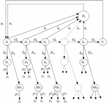
Based on the two-state model, the component model with deterioration and random failure is developed using Markov processes. Transitions from the deterioration state to maintenance states (both minor and major) are also incorporated. Deterioration (D) of the component is modeled as occurring in k discrete steps. The failure types, namely deterioration failure (F1) and random failure (F0), are considered. The state space diagram is shown in Figure 1.

State space diagram for the component model.
Preventive maintenance leads to an improvement in the deterioration chain; however, allowances are made for the cases where no improvement is achieved. For instance, in the case of minor preventive maintenance being performed, the component improves from stage i to stage i − 1 of deterioration or remains in the same deterioration stage i. In the case of major preventive maintenance being performed, the component improves from stage i to stage i − 2 of deterioration, to stage i − 1 of deterioration, or remains in the same deterioration stage I [1]. If the component is in stage 1 of deterioration, it remains in that stage on completion of either minor or major preventive maintenance.
As a result of preventive maintenance, the probabilities of transitions from minor or major maintenance states to deteriorations states D1, D2,…, or Dk are different. Transitions from each deterioration stage to both minor and major maintenance states occur at rates λm and λm1 correspondingly. For simplicity, consider λm = kλ λm1, where kλ is the proportionality constant. The mean duration to minor maintenance and major maintenance are 1/μm and 1/μm1, respectively. Repairs following random failure and deterioration failure are completed at rates of μ0 and μ1, respectively.
The values of λ0, λ1, μ0, μ1, μm, and μm1 are obtained from the past outage statistics and maintenance practices, and they represent average values. The steady state solution of the component model is obtained by using a recursive approach. The recursive algorithm computes the steady state probabilities of the component [10]. The availability A(λm), which is defined as the probability that the component is in service, is given by A(λm) = P1 + P2 + P3 where P1, P2, and P3 are the steady state probabilities of the component being in service.
The optimal values of mean time to maintenance (minor and major) are determined by maximizing the availability of the component. Mathematical optimization programs such as Maple 7 and Lingo 7 programs can be used for the optimization of the model. The solution yields the optimal mean time to minor maintenance (1/λm*), and from the relation λm = kλ λm1, the optimal mean time to major maintenance (1/λm1*) is obtained.
3. MARKOV DECISION PROCESSES
Using the state probabilities found in the previous section, the optimal maintenance policy can be determined by setting up the component model as a MDP. At every deterioration stage, a decision process involving a choice from three possible actions, namely do nothing, do minor maintenance, and do major maintenance, is made. The objective is to obtain an optimal policy to select the best action in each state in order to maximize the long-run average return.
In general, an MDP comprises the following:
- State space, S = {si |, i = 1,2,…,n}, where n is assumed to be finite;
- Action space that defines actions that may be taken over a state space, A = {A(s) | ∀ s ∈ S}, where A(s) is a finite set of actions defined on states.
- Probabilistic state transition function, P(i,k,j), which describes the probability of making a state transition from any one arbitrary state i to a state jj, when an action k defined on A(i) is taken.
- Reward function (or cost function) R(i,k,j) over the problem space, which specifies an instant reward that will be received after an action is performed (under a corresponding state transition). These values are predicted from the cost of various maintenance activities and/or their consequences.
A decision rule prescribes a procedure for action selection in each state at a specified decision epoch [8]. A policy is a sequence of decision rules to be used at all decision epochs for a specified time horizon that can be finite or infinite. A stationary policy is a policy where the decision rule is the same in every decision epoch.
If P(j|i,k) represents the transition probability from state i to state j as a result of action k, and r(i,k,j) represents the return that results due to a transition from state i to state j as a result of action k, then the expected return as a result of action k while in state i is given by

Based on the state of a process at any time and the action chosen, an expected reward is earned and the probability distribution for the next state is determined. The objective is to choose a policy that maximizes the expected value of the sum of the rewards earned over a given finite time period. In this paper, Linear Programming is used to determine the optimal maintenance policy.
Linear programming algorithm [8]
Step 1. Apply the simplex method to compute an optimal basic solution (xia*) to the linear program.
Minimize

subject to

Step 2. Start with the nonempty set,

and, for any state i ∈ T, set the decision Ri* = a for some a such that xia* > 0.
Step 3. If T = S, then stop the algorithm with the average cost optimal policy R*. Otherwise, determine some state i ∉ T and action a ∈ A(i) such that pij(a) > 0 for some j ∈ T and set Ri* = a and T = T ∪ {i}. Repeat Step 3.
4. NUMERICAL EXAMPLE
The implementation of the model is illustrated with the following example. Consider a unit for which the average random failure occurs once in 500 days and that the repair lasts for 7 days. If the unit is not maintained, it would fail from deterioration on an average of every 1000 days and the mean repair time is 14 days. Also, the minor maintenance would take an average of half a day and the major maintenance would take an average of 1 day. Assume that all times are exponentially distributed and the number of stages of deterioration of the unit is 3. Hence, the input parameters are as follows:

The steady state equations and the input parameters are utilized to obtain the optimal solution using both Maple 7 and Lingo 7 programs. The results obtained are as given below.
In order to find the optimal policy, the best action must be chosen in each state. Action I refers to “do nothing,” action II refers to “do minor maintenance,” and action III refers to “do major maintenance.”
State space:

Action space:

Actions I, II, and III can be chosen in states D1, D2, and D3, whereas only Action I is available in states M1, M2, M3, MM1, MM2, MM3, F0, and F1. Therefore, the action sets are as follows:

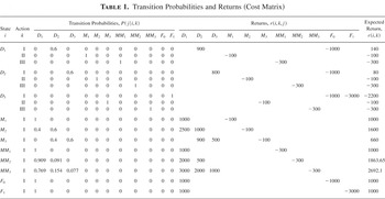
The returns are assigned based on the level of deterioration and maintenance state. For instance, the reward for a transition from D1 to D2 is chosen to be 900 and that from D2 to D3 is 800. The reward decreases because the component is deteriorating and does not work as efficiently. The reward for the component to stay in states M1, M2, and M3 is −100; for states MM1, MM2, and MM3, it is −300; for state F0, it is −1000; for state F1, it is −3000 (Case I). The returns in these states are based on the duration of unavailability of the component; the longer the component is out of service either for maintenance or repair of failures, the greater the loss. Also, the return for a transition from any of the maintenance states (minor or major) to state D1 is greater than the return resulting from a transition to state D2. This is because there is more improvement in the deterioration chain in state D1 than in state D2. Likewise, the return for a transition from any of the maintenance states (minor or major) to state D2 is greater than the return resulting from a transition to state 3. Also, positive values of returns indicate reward earned and negative values of returns indicate cost incurred. The probabilities are calculated using the transition rates in the component model. Using the transition probabilities and rewards, the cost matrix is obtained as shown in Table 1. The optimal policy algorithms are used to find the optimal maintenance policy for the component model. An APL language software called MDP is utilized for Linear Programming and solving the model [2].
Transition Probabilities and Returns (Cost Matrix)

The model was also tested with a different set of values for rewards (Case II). The rewards for the transition from failure state F0 to D1 as a result of action {do nothing} is chosen to be 3000 and the reward for transition from failure state F1 to D1 as a result of action {do nothing} is also chosen to be 3000. All other values are chosen to be the same as before.
5. RESULTS
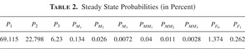
Table 2 provides the steady state probabilities (in percent) for different states of the component. The availability of the component is calculated to be 0.9814316. The optimal values of the mean times to minor preventive maintenance and major preventive maintenance for the component model are calculated as 86 days and 172 days, respectively, for a mean time to random failure of 500 days. As expected, the availability decreases as the mean times to preventive maintenance (minor and major) exceed the optimal value.
Steady State Probabilities (in Percent)

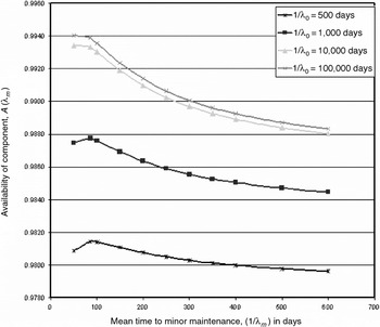
Figure 2 illustrates the effect of varying mean time to random failure (λ0−1) for the component model. For a specified value of λ0−1, the mean times to maintenance corresponding to maximum availability can be determined. For example, for a mean time to random failure (λ0−1) of 500 days, the optimal values of the mean times to minor maintenance and major maintenance are 86 days and 172 days, respectively, and the maximum availability of the component is 0.98143. The availability decreases as the mean times to maintenance (minor and major) exceed the optimal value, as expected. The optimal values for mean times to maintenance (minor and major) and corresponding maximum availability by varying mean times to random failure (λ0−1) can also be seen in Figure 2.

Effect of varying mean time to random failure. Note: For 1/λ1 = 1000 days; 1/μ1 = 14 days.
By increasing λ0−1, the optimal values of mean times to maintenance (both minor and major) decrease. It is also observed that the availability of component increases as λ0−1 increases. This is because by increasing λ0−1 (i.e., decrease in random failure rate), more frequent maintenance is needed to bring the component to the new status and, hence, there is higher component availability. By increasing the value of μ0−1, availability reduces, due to the fact that as more time is spent on repairing random failures (i.e., increasing μ0−1), the availability of the component reduces. If all parameters remain unchanged, increasing μ1−1 will decrease the value of λm−1 and will reduce the availability of the component. This is because by increasing the repair time for deterioration failure (i.e., increasing μ1−1), the availability of the component reduces.
Optimal Policy
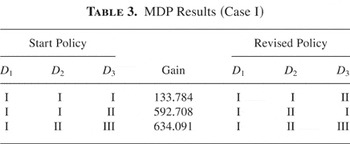
Using MDPs, the optimal policy obtained in deterioration states D1, D2, and D3 consists of actions {do nothing}, {do minor maintenance}, and {do major maintenance}, respectively, for Case I. The optimal policy yields an average cost per stage equal to 634, as shown in Table 3.
MDP Results (Case I)

In Case II, it is assumed that the reward for transition from failure states to D1 as a result of action {do nothing} is 3000, as opposed to 1000 (in Case I). All other values are chosen to be the same as in Case I. The results for Case II consist of actions {do nothing}, {do nothing}, and {do major maintenance} for states D1, D2, and D3, respectively. The gain for this policy is 1009.
6. CONCLUSION
For the component model, with three levels of deterioration, the optimal maintenance policy indicates that in the initial level of deterioration, there is no need for preventive maintenance, whereas in the intermediate level of deterioration, minor maintenance is to be carried out, and in the crucial level of deterioration, major maintenance is to be performed. This optimal policy yields maximum long-run average return and contributes to the reliable operation of the component.
A more realistic maintenance model has been developed by incorporating deterioration and both types of failure. The solution for determining optimal mean times to preventive maintenance is fairly simple and can be done through simple nonlinear optimization algorithms.
References
REFERENCES
Anders, G.J.
(1990).
Probability concepts in electric power systems.
New York:
Wiley.
APL website,
http://asrl.ecn.uiowa.edu/dbricker/APL_Software.html.
Asgarpoor, S. &
Doghman, M.
(1999).
A maintenance optimization program for utilities' transmission
and distribution systems. In
Proceedings of the 1999 North American Power Symposium, pp.
454–459.
Chan, G.K.
(1998).
Preventive maintenance with Markov processes.
M.E. thesis,
University of Nebraska–Lincoln,
Lincoln NE.
Dekker, R.
(1996).
Applications of maintenance optimization models: A review and
analysis.
Reliability Engineering and System Safety
51:
229–240.Google Scholar
Endrenyi, J.,
Anders, G.J., &
Leite da Silva, A.M.
(1998).
Probabilistic evaluation of the effect of maintenance on
reliability: An application.
IEEE Transactions on Power Systems
13(2):
576–583.Google Scholar
Endrenyi, J.,
et al.
(IEEE/PES Task Force on Impact of Maintenance Strategy on
Reliability).
(2000).
The present status of maintenance strategies and the impact of
maintenance on reliability.
IEEE Transactions on Power Systems
16(4):
638–646.Google Scholar
Puterman, M.L.
(1994).
Markov decision processes: Discrete stochastic dynamic
programming.
New York:
Wiley.
Sim, S.H. &
Endrenyi, J.
(1988).
Optimal preventive maintenance with repair.
IEEE Transactions on Reliability
37(1):
92–96.Google Scholar
Sim, S.H. &
Endrenyi, J.
(1993).
A failure repair model with minimal and major maintenance.
IEEE Transactions on Reliability
42(1):
134–139.Google Scholar
State space diagram for the component model.
Transition Probabilities and Returns (Cost Matrix)
Steady State Probabilities (in Percent)
Effect of varying mean time to random failure. Note: For 1/λ1 = 1000 days; 1/μ1 = 14 days.
MDP Results (Case I)
 You have
Access
- 12
- Cited by